A Classification of Hidden-Variable Properties∗

Adam Brandenburger† Noson Yanofsky‡

First Version 01/04/07Current Version 08/18/08

Abstract

Hidden variables are extra components added to try to banish counterintuitive features of

quantum mechanics. We start with a quantum-mechanical model and describe various properties

that can be asked of a hidden-variable model. We present six such properties and a Venn diagram

of how they are related. With two existence theorems and three no-go theorems (EPR, Bell, and

Kochen-Specker), we show which properties of empirically equivalent hidden-variable models are

possible and which are not. Formally, our treatment relies only on classical probability models,

and physical phenomena are used only to motivate which models to choose.

1 Introduction

Begun by von Neumann [34, 1932], the hidden-variable program in quantum mechanics (QM) addsextra (“hidden”) ingredients in order to try to banish some of the counterintuitive features of QM.These features are: (i) the probabilistic nature of quantum behavior, (ii) the possibility of so-callednon-local effects between widely separated particles, and (iii) the idea of an intrinsic dependencebetween the observer of a QM system and the properties of the system itself.

Hidden-variable theories aim to remove these strange aspects of QM by building more “com-plete” models (in the terminology of Einstein-Podolsky-Rosen [16, 1935]). The completed modelsshould agree with the predictions of QM, but exhibit one or more of the desired properties of: (i)determinism, (ii) locality, and (iii) independence.

Can such models actually be built? The famous “no-go” theorems of QM show that there aresevere limitations to what can be done. But it is also true that certain combinations of propertiesare possible.∗We are indebted to Shelly Goldstein for detailed and valuable comments on an earlier draft. Our thanks to

Amanda Friedenberg, Alex Peysakhovich, Gus Stuart, Jean de Valpine, and three anonymous referees for importantinput, and to Michael Giangrasso for technical assistance. Financial support from the Stern School of Business isgratefully acknowledged. chvp-08-18-08†Address: Stern School of Business, New York University, 44 West Fourth Street, New York, NY 10012,

adam.brandenburger@stern.nyu.edu, www.stern.nyu.edu/∼abranden‡Address: Department of Computer and Information Science, Brooklyn College, 2900 Bedford Avenue, Brooklyn,

NY 11210, noson@sci.brooklyn.cuny.edu, www.sci.brooklyn.cuny.edu/∼noson

arX

iv:0

711.

4650

v2 [

quan

t-ph

] 2

0 A

ug 2

008

Our modest goal in this paper is to provide a formal framework in which various properties onemight ask of hidden-variable models can be stated and in which various non-existence and existenceresults can be organized. Almost all–if not all–of the ingredients of what we do in this paper arewell known to researchers in the area. Our contribution, we hope, is in putting all the ingredientsinto one simple setting.

The setting is classical probability spaces. The question is, given a classical probability model,whether there exists an associated hidden-variable model that is empirically equivalent to the firstmodel and that satisfies certain properties. These properties are motivated by the literature onhidden variables in QM. The specific properties we consider–and the relationships among them–canbe depicted in the Venn diagram of Figure 1.1. (We define all the terms later.) The diagram contains21 regions.

Figure 1.1

The main result of the paper is that we can give a complete account of these 21 regions. For 10of these regions (indicated with checks), it is always possible to find an equivalent hidden-variablemodel with the properties in question. For the remaining 11 regions (indicated with crosses), thismay not be possible. We fill in the regions via two existence results and three non-existence results.The latter three are the famous theorems of Einstein-Podolsky-Rosen (EPR) [16, 1935],1 Bell [2,

1Strictly speaking, EPR did not state a non-existence theorem, but it is useful to present their argument this way.

2

1964], and Kochen-Specker [24, 1967].It is important to understand that, formally, our paper makes no use of physical phenomena.

It is an exercise in classical probability theory alone. Of course, the probability spaces we selectfor the non-existence results are inspired by the physical experiments described in EPR, Bell, andKocher-Specker. But we hope it is conceptually clarifying to present the hidden-variable questionin a purely abstract setting–that is, to show how much follows from the rules of probability theoryalone.

Naturally, our account of hidden-variable theory is complete only relative to the properties weconsider (there are six of them). These properties are, as far as we can tell, the main ones consideredin the literature. (As we explain later, we have added one definition.) In particular, Bell Locality ([2,1964]) is equivalent to the conjunction of Outcome and Parameter Independence (Jarrett [23, 1984],stated here as Proposition 2.1). Kochen-Specker [24, 1967] Non-Contextuality is implied by theconjunction of Parameter Independence and λ-Independence (Proposition 2.2). But there may wellbe other interesting properties to put on hidden-variable models, which would lead to an extensionof Figure 1.1.

There are, of course, many treatments of the hidden-variable question. (Prominent examplesinclude Belifante [1, 1973], Gudder [21, 1988], Mermin [26, 1993], Peres [28, 1990], and van Fraassen[33, 1991].) This paper is not meant to be a comprehensive survey. Our goal is, in a sense, thereverse. It is to start with the rules of probability theory alone and ask–relative to the six propertieswe consider–what is or is not possible. For this task, we need only EPR, Bell, and Kochen-Specker.But we do mention later some other no-go results in QM (not needed to complete Figure 1.1).

Two comments on the particular framework we present. First, we work with a single probabil-ity measure on a single space, where points in the space describe measurements on particles andoutcomes of those measurements. An alternative–more conventional–approach would be to use afamily of probability measures on a space describing outcomes only, with different probability mea-sures corresponding to different measurements.2 In fact, all our requirements are stated in terms ofconditional probabilities: If such-and-such a measurement is made, then what is the probability of acertain outcome? The distinction between the approaches might therefore seem small–both involvefamilies of probability measures. But it matters. If we had started from a family of probabilitymeasures rather than a single measure, we would not have been able to derive all the relationshipsbetween properties shown in Figure 2.1 without making some additional assumptions.3 So, formally,our approach is more parsimonious. Yet, it does add an ingredient at the conceptual level–viz., theexistence of a probability measure prior to conditioning on measurements. This measure may bethought of as representing the perspective of a super-observer who observes the experimenters aswell as the outcomes of the experiments. Does the existence of such a measure contradict the freewill of an experimenter in deciding what measurements to make? We don’t think so–because, as we

2We are grateful to Shelly Goldstein and a referee who both pointed to this issue.3A reader preferring the more conventional approach can simply make these additional assumptions. We give

details in the next section.

3

said, we work only with the conditionals. Still, even if it plays a very small role in our treatment,the idea of such a measure seems deserving of further study. We leave this as beyond the scope ofthe current paper.

A second choice we make in our framework is to treat only finite probability spaces. This involvesa tradeoff. On the one hand, finiteness allows us to avoid all measure-theoretic issues. On the otherhand, as an assumption on the space in which a hidden variable lives, finiteness is undoubtedlyrestrictive. To be precise, the first of our two existence theorems needs only a finite space in anycase, but, under finiteness, the second can treat only rational probabilities. (We sketch the extensionof our second theorem, using an infinite space, to all probabilities.) Of course, finiteness makes ourversions of the no-go theorems weaker.

We derive Figure 1.1 in the body of the paper. Before that, though, let us offer a commenton its conceptual meaning in QM. The main message of the no-go theorems is that in building ahidden-variable theory, some properties that might be viewed as desirable–at least, a priori–have tobe given up. But there is a choice of what to give up. Arguably, it is more a matter of metaphysicsthan physics as to what choice to make. The point of a formal treatment–as in Figure 1.1–is to givea precise statement of what the options are. There is a basic three-way tradeoff. We can have:

(i) Determinism (As we will explain, this comes in a strong or a weak form.) This says thatrandomness reflects only observer ignorance. Once hidden variables are introduced, there isno residual randomness in the universe.

(ii) Parameter Independence This says that when conducting an experiment on a system ofparticles, the outcome of a measurement on one of the particles does not depend on whatmeasurements are performed on other particles. (The intuitive appeal of this property is thatoften the particles are widely separated.) This is a way of saying that the universe is local.

(iii) λ-Independence This says that the nature of the particles–as determined by the value ofa hidden variable–does not depend on the experiment conducted. There is, in this sense, nodependence between the observer and the observed.

Any one of these properties is consistent with the predictions of QM. So are certain combinationsof properties, as Figure 1.1 shows. But, however a priori reasonable they may seem, we cannot haveall three properties–or even certain pairs of properties. There is an inherent tradeoff. This is aninescapable feature of QM.

The rest of the paper is organized as follows. Section 2 lays out the framework and basicdefinitions. Section 3 presents two existence theorems on hidden-variable models. Sections 4-6present EPR [16, 1935], Bell [2, 1964], and Kochen-Specker [24, 1967] in our probability-theoreticframework. Section 7 mentions some other impossibility results in QM not covered in this paper.

4

2 The Models and Their Properties

Here is the hidden-variable question in a bit more detail. Start with a model of an experiment donein QM. Sometimes, the experiment will consist of measurements performed on several entangledparticles. Or, the experiment might involve several measurements performed on a single particle.The model describes the set-up and outcome of the experiment and so will be called an “empiricalmodel.” The question is whether one can find a hidden-variable model–i.e., a model involvingadditional (“hidden”) variables–which is empirically equivalent to the first model and which hasdesired properties. By “empirically equivalent” we mean that the two models make the same(probabilistic) prediction about outcomes.

Formally, we consider a space

Ψ = a, a′, . . . × b, b′, . . . × c, c′, . . . · · · × A,A′, . . . × B,B′, . . . × C,C ′, . . . × · · · .

The variables A,B,C, . . . are measurements, and the variables a, b, c, . . . are associated outcomesof measurements. There might be several particles: Ann performs a measurement on her particle,Bob performs a measurements on his particle, . . . . Or, Ψ might describe a case where severalmeasurements are performed on one particle. The definitions to come apply in either case. Wetake each of the spaces in Ψ to be finite, and suppose that Ψ is a finite product.

Let Λ be a finite space in which a hidden variable λ lives.4 The overall space is then

Ω = Ψ× Λ.

Definition 2.1 An empirical model is a pair (Ψ, q), where q is a probability measure on Ψ. Ahidden-variable model is a pair (Ω, p), where p is a probability measure on Ω.

Essentially, we employ the probability measures q and p once conditioned on one or more mea-surements. Still, as we said in the Introduction, we cannot quite dispense with the unconditional qand p, and work instead with a family of probability measures indexed by measurements (one familyfor q and one for p). If we did, we would lose Lemmas 2.1 and 2.4–and hence certain relationshipsin Figure 1.1. These relationships seem intuitively correct to us, so we prefer a formalism in whichthey can be derived. With an indexed family of measures, we would have to impose rather thanderive these relationships.

The models of Definition 2.1 stand alone. However, we are also interested in stating whendifferent models are equivalent:

Definition 2.2 An empirical model (Ψ, q) and a hidden-variable model (Ω, p) are (empirically)

4Throughout, we talk about one hidden variable. But we put no structure on the space in which the hiddenvariable lives. Of course, in the infinite case, a measurable structure would be needed.

5

equivalent if for all a, b, c, . . . , A,B,C, . . . ,

q(A,B,C, . . .) > 0 if and only if p(A,B,C, . . .) > 0,

and when both are non-zero,

q(a, b, c, . . . |A,B,C, . . .) = p(a, b, c, . . . |A,B,C, . . .).

Here, we write “a, b, c, . . .” as a shorthand for the event

(a, b, c, . . .) × A,A′, . . . × B,B′, . . . × C,C ′, . . . × · · ·

in Ψ, or the event

(a, b, c, . . .) × A,A′, . . . × B,B′, . . . × C,C ′, . . . × · · · × Λ

in Ω, and similarly for other expressions. We will adopt this shorthand throughout.The non-nullness condition is simply to ensure that any measurements (A,B,C, . . .) which are

possible in the empirical model are also possible in the hidden-variable model under consideration,and vice versa. Without this condition, it would be hard to compare the two models.

We will often calculate p(a, b, c, . . . |A,B,C, . . .), for p(A,B,C, . . .) > 0, from the formula:

p(a, b, c, . . . |A,B,C, . . .) =∑

λ:p(A,B,C,...,λ)>0

p(a, b, c, . . . |A,B,C, . . . , λ)p(λ|A,B,C, . . .).

Substituting this in Definition 2.2, we see that the idea of equivalence is to reproduce a givenprobability measure q on the space Ψ by averaging under a probability measure p on an augmentedspace Ω, where Ω includes a hidden variable. The measure p is then subject to various conditions(described below).

One more basic definition:

Definition 2.3 Two hidden-variable models (Ω, p) and (Ω, p) are (empirically) equivalent if forall a, b, c, . . . , A,B,C, . . . ,

p(A,B,C, . . .) > 0 if and only if p(A,B,C, . . .) > 0,

and when both are non-zero,

p(a, b, c, . . . |A,B,C, . . .) = p(a, b, c, . . . |A,B,C, . . .).

Now, we move on to the different properties of hidden-variable models. Figure 2.1 repeatsFigure 1.1 (without the checks and crosses), as a preview of the properties and relationships we will

6

consider.

Figure 2.1

Definition 2.4 A hidden-variable model (Ω, p) satisfies Single-Valuedness if Λ is a singleton.

This condition says that the hidden variable can take on only one value. In effect, this conditiondoesn’t allow hidden variables. We include it because EPR will be usefully formulated this way.

Definition 2.5 A hidden-variable model (Ω, p) satisfies λ-Independence if for all A,A′, B,B′, C, C ′,. . ., λ, whenever

p(A,B,C, . . .) > 0 and p(A′, B′, C ′, . . .) > 0,

thenp(λ|A,B,C, . . .) = p(λ|A′, B′, C ′, . . .).

(This term is from Dickson [14, 2005, p.140].) The condition says that the process determiningthe value of the hidden variable is independent of which measurements are chosen.

Remark 2.1 If a hidden-variable model satisfies Single-Valuedness, then it satisfies λ-Independence.

Definition 2.6 A hidden-variable model (Ω, p) satisfies Strong Determinism if, for every A, λ,whenever p(A, λ) > 0, there is an a such that p(a|A, λ) = 1, and similarly for B, λ, b, etc.

7

Definition 2.7 A hidden-variable model (Ω, p) satisfies Weak Determinism if, for every A,B,C,. . . , λ, whenever p(A,B,C, . . . , λ) > 0, there is a tuple a, b, c, . . . such that p(a, b, c, . . . |A,B,C, . . . , λ) =1.

Determinism is a basic condition in the literature. But we are careful to make a distinctionbetween a strong and weak form. We will see that various results are true for one form but false foranother. Broadly, the condition is that the hidden variable determines (almost surely) the outcomesof measurements. But, Strong Determinism says this holds measurement-by-measurement, whileWeak Determinism says this holds only once all measurements are specified. There is a one-wayimplication:

Lemma 2.1 If a hidden-variable model satisfies Strong Determinism, then it satisfies Weak Deter-minism.

Proof. Suppose p(A,B,C, . . . , λ) > 0. Then p(A, λ) > 0, p(B, λ) > 0, p(C, λ) > 0, . . . . So, thereare a, b, c, . . . , such that p(a|A, λ) = 1, p(b|B, λ) = 1, p(c|C, λ) = 1, . . . .

The result now follows from the following easy fact in probability theory: Let E1, . . . , En andF1, . . . , Fn be events with p(

⋂i Fi) > 0. If p(Ei|Fi) = 1 for all i, then p(

⋂iEi|

⋂i Fi) = 1.

Definition 2.8 A hidden-variable model (Ω, p) satisfies Outcome Independence if for all a, b, c,. . . , A,B,C,. . . , λ, whenever p(A,B,C, . . . , b, c, . . . , λ) > 0,

p(a|A,B,C, . . . , b, c, . . . , λ) = p(a|A,B,C, . . . , λ), (2.1)

and similarly with a and b interchanged, etc.

Outcome Independence is taken from Jarrett [23, 1984] and Shimony [30, 1986]. It says thatconditional on the value of the hidden variable and the measurements undertaken, the outcome ofany one measurement is (probabilistically) unaffected by the outcomes of the other measurements.

Lemma 2.2 A hidden-variable model (Ω, p) satisfies Outcome Independence if and only if for alla, b, c, . . . , A,B,C,. . . , λ, whenever p(A,B,C, . . . , λ) > 0,

p(a, b, c, . . . |A,B,C, . . . , λ) = p(a|A,B,C, . . . , λ)× p(b|A,B,C, . . . , λ)× p(c|A,B,C, . . . , λ)× · · · .(2.2)

Proof. Standard; see, e.g., Chung [9, 1974, Theorem 9.2.1].

Lemma 2.3 (Bub [7, 1997, p.69]) If a hidden-variable model satisfies Weak Determinism, thenit satisfies Outcome Independence.

Proof. Suppose p(A,B,C, . . . , λ) > 0. Then, by Weak Determinism, there is a tuple a∗, b∗, c∗, . . .such that

8

p(a, b, c, . . . |A,B,C, . . . , λ) = χa=a∗ × χb=b∗ × χc=c∗ × · · · .

But then p(a|A,B,C, . . . , λ) = χa=a∗, p(b|A,B,C, . . . , λ) = χb=b∗, p(c|A,B,C, . . . , λ) =χc=c∗, . . . . Now use Lemma 2.2.

Definition 2.9 A hidden-variable model (Ω, p) satisfies Parameter Independence if for all a,A,B,C,. . . , λ, whenever p(A,B,C, . . . , λ) > 0,

p(a|A,B,C, . . . , λ) = p(a|A, λ), (2.3)

and similarly for b, A,B,C, . . . , λ, etc.

Parameter Independence is also from Jarrett [23, 1984] and Shimony [30, 1986]. It says that,conditional on the value of the hidden variable, the outcome of any one measurement depends(probabilistically) only on that measurement and not on the other measurements.

Lemma 2.4 If a hidden-variable model satisfies Strong Determinism, then it satisfies ParameterIndependence.

Proof. Suppose p(A,B,C, . . . , λ) > 0. Then p(A, λ) > 0. So, by Strong Determinism, thereis an a∗ such that p(a|A, λ) = χa=a∗. But p(a,A,B,C, . . . , λ|A, λ) = p(a|A,B,C, . . . , λ) ×p(A,B,C, . . . , λ|A, λ), where p(A,B,C, . . . , λ|A, λ) > 0. From p(a∗|A, λ) = 1, p(a∗, A,B,C, . . . , λ|A, λ)= p(A,B,C, . . . , λ|A, λ). From p(a|A, λ) = 0 when a 6= a∗, we get p(a,A,B,C, . . . , λ|A, λ) = 0.Thus, p(a|A,B,C, . . . , λ) = χa=a∗, establishing (2.3).

Combinations of some of these properties give the well-known properties of Locality and Non-Contextuality. First is Locality, formulated by Bell [2, 1964]. In words, a hidden-variable modelsatisfies Locality if the probability of getting some tuple of outcomes factorizes under the measure-ments.

Definition 2.10 A hidden-variable model (Ω, p) satisfies Locality if for all a, b, c, . . . , A,B,C,,. . . , λ, whenever p(A,B,C, . . . , λ) > 0,

p(a, b, c, . . . |A,B,C, . . . , λ) = p(a|A, λ)× p(b|B, λ)× p(c|C, λ)× · · · . (2.4)

Proposition 2.1 (Jarrett [23, 1984, p.582]) A hidden-variable model satisfies Locality if andonly if it satisfies Outcome Independence and Parameter Independence.

Proof. Assume p(A,B,C, . . . , λ) > 0, and substitute (2.3) and its counterparts into (2.2). Thisyields (2.4).

Conversely, assume again p(A,B,C, . . . , λ) > 0, and sum both sides of (2.4) over b, c, . . . . Thisyields (2.3). Moreover, substituting (2.3) and its counterparts into (2.4) yields (2.2).

9

Non-Contextuality, due to Kochen-Specker [24, 1967], is a property of an empirical model. Itsays that the probability of obtaining a particular outcome of a measurement does not depend onthe other measurements performed.

Definition 2.11 An empirical model (Ψ, q) satisfies Non-Contextuality if for all a,A,B,B′, C, C ′,. . . , whenever q(A,B,C, . . .) > 0 and q(A,B′, C ′, . . .) > 0,

q(a|A,B,C, . . .) = q(a|A,B′, C ′, . . .).

Also, the corresponding conditions must hold for b, A,A′, B, C,C ′, . . ., etc.

Proposition 2.2 If a hidden-variable model (Ω, p) satisfies λ-Independence and Parameter Inde-pendence, then any equivalent empirical model (Ψ, q) satisfies Non-Contextuality.

Proof. We can assume p(A,B,C, . . .) > 0 and p(A,B′, C ′, . . .) > 0. Then

p(a|A,B,C, . . .) =∑

λ:p(A,B,C,...,λ)>0

p(a|A,B,C, . . . , λ)p(λ|A,B,C, . . .) =

∑λ:p(A,B,C,...,λ)>0

p(a|A,B,C, . . . , λ)p(λ) =

∑λ:p(A,B,C,...,λ)>0

p(a|A, λ)p(λ),

where the second line uses λ-Independence and the third line uses Parameter Independence. Usingp(A,B,C, . . .) > 0 and λ-Independence again, we have p(A,B,C, . . . , λ) > 0 if and only if p(λ) > 0.So

p(a|A,B,C, . . .) =∑

λ:p(λ)>0

p(a|A, λ)p(λ).

A similar argument establishes

p(a|A,B′, C ′, . . .) =∑

λ:p(λ)>0

p(a|A, λ)p(λ),

so that p(a|A,B,C, . . .) = p(a|A,B′, C ′, . . .), as required.

3 Two Existence Theorems

We next prove two existence theorems for hidden-variable models which say what type of propertiescan always be found:

E1 Given any empirical model, there is an equivalent hidden-variable model which satisfies StrongDeterminism.

10

E2 Given any empirical model, there is an equivalent hidden-variable model which satisfies WeakDeterminism and λ-Independence.

That is, each of these sets of conditions on a hidden-variable theory can always be satisfied.They cannot be impeded by any no-go theorems. Figure 3.1 repeats part of Figure 1.1, putting acheck in a region where there is always an equivalent hidden-variable model with the properties thathold in that region. The checks are followed by E1 and/or E2 which say which existence theorempertains to that region.

(The region for Single-Valuedness alone also has a check. The existence of an equivalent hidden-variable model satisfying Single-Valuedness alone is immediate–it is essentially just the given empir-ical model. See Remark 3.1 for a statement.)

Figure 3.1

Here are the two existence theorems. Similar methods to those in the first proof can be foundin Fine [17, 1982, p.292]. The idea of the second theorem is in Teufel-Berndl-Durr-Goldstein-Zanghı [32, 1997, p.1219] (see also Werner and Wolf [36, 2001, p.7]). But we have not found exactstatements of the two theorems in the literature.

Theorem 3.1 Given an empirical model (Ψ, q), there is an equivalent hidden-variable model (Ω, p)which satisfies Strong Determinism.

11

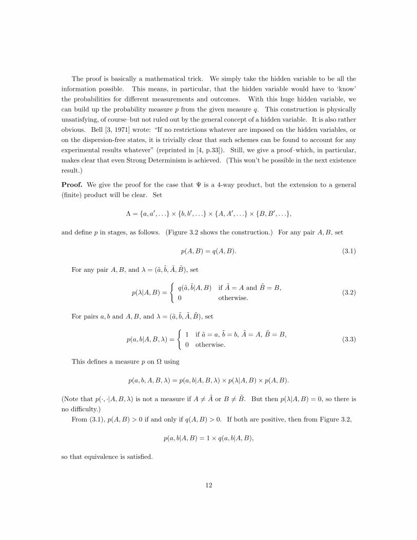
The proof is basically a mathematical trick. We simply take the hidden variable to be all theinformation possible. This means, in particular, that the hidden variable would have to ‘know’the probabilities for different measurements and outcomes. With this huge hidden variable, wecan build up the probability measure p from the given measure q. This construction is physicallyunsatisfying, of course–but not ruled out by the general concept of a hidden variable. It is also ratherobvious. Bell [3, 1971] wrote: “If no restrictions whatever are imposed on the hidden variables, oron the dispersion-free states, it is trivially clear that such schemes can be found to account for anyexperimental results whatever” (reprinted in [4, p.33]). Still, we give a proof–which, in particular,makes clear that even Strong Determinism is achieved. (This won’t be possible in the next existenceresult.)

Proof. We give the proof for the case that Ψ is a 4-way product, but the extension to a general(finite) product will be clear. Set

Λ = a, a′, . . . × b, b′, . . . × A,A′, . . . × B,B′, . . .,

and define p in stages, as follows. (Figure 3.2 shows the construction.) For any pair A,B, set

p(A,B) = q(A,B). (3.1)

For any pair A,B, and λ = (a, b, A, B), set

p(λ|A,B) =

q(a, b|A,B) if A = A and B = B,0 otherwise.

(3.2)

For pairs a, b and A,B, and λ = (a, b, A, B), set

p(a, b|A,B, λ) =

1 if a = a, b = b, A = A, B = B,0 otherwise.

(3.3)

This defines a measure p on Ω using

p(a, b, A,B, λ) = p(a, b|A,B, λ)× p(λ|A,B)× p(A,B).

(Note that p(·, ·|A,B, λ) is not a measure if A 6= A or B 6= B. But then p(λ|A,B) = 0, so there isno difficulty.)

From (3.1), p(A,B) > 0 if and only if q(A,B) > 0. If both are positive, then from Figure 3.2,

p(a, b|A,B) = 1× q(a, b|A,B),

so that equivalence is satisfied.

12

Figure 3.2

It remains to verify that (Ω, p) satisfies Strong Determinism. So, suppose p(A, λ) > 0. Writingλ = (a, b, A, B), we therefore assume A = A. Using (3.1)-(3.3),

p(a,A, λ) = p(a, A, λ) =∑b′,B′

p(a, b′, A, B′, λ) = p(a, b, A, B, λ) = q(a, b, A, B)× χa=a,

p(A, λ) = p(A, λ) =∑

a′,b′,B′

p(a′, b′, A, B′, λ) = p(a, b, A, B, λ) = q(a, b, A, B),

so thatp(a|A, λ) = χa=a,

which is Strong Determinism.

Corollary 3.1 Given a hidden-variable model (Ω, p), there is an equivalent hidden-variable model(Ω, p) which satisfies Strong Determinism.

Proof. Start with (Ω, p), and (partially) define an equivalent empirical model (Ψ, q) by

q(a, b|A,B) =∑

λ:p(A,B,λ)>0

p(a, b|A,B, λ)p(λ|A,B),

for p(A,B) > 0. (There is no difficulty in completing the definition of q.)By Theorem 3.1, there is a hidden-variable model (Ω, p) which is equivalent to (Ψ, q) and which

satisfies Strong Determinism. But (Ω, p) is also equivalent to (Ω, p).

13

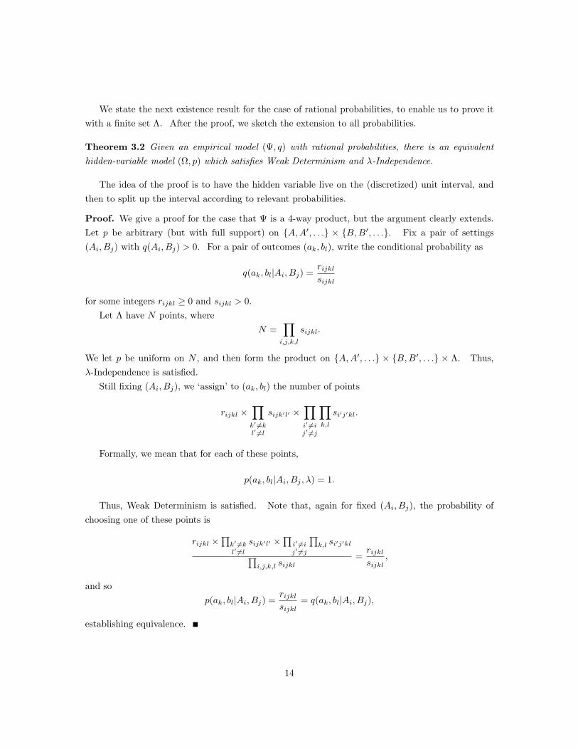
We state the next existence result for the case of rational probabilities, to enable us to prove itwith a finite set Λ. After the proof, we sketch the extension to all probabilities.

Theorem 3.2 Given an empirical model (Ψ, q) with rational probabilities, there is an equivalenthidden-variable model (Ω, p) which satisfies Weak Determinism and λ-Independence.

The idea of the proof is to have the hidden variable live on the (discretized) unit interval, andthen to split up the interval according to relevant probabilities.

Proof. We give a proof for the case that Ψ is a 4-way product, but the argument clearly extends.Let p be arbitrary (but with full support) on A,A′, . . . × B,B′, . . .. Fix a pair of settings(Ai, Bj) with q(Ai, Bj) > 0. For a pair of outcomes (ak, bl), write the conditional probability as

q(ak, bl|Ai, Bj) =rijklsijkl

for some integers rijkl ≥ 0 and sijkl > 0.Let Λ have N points, where

N =∏i,j,k,l

sijkl.

We let p be uniform on N , and then form the product on A,A′, . . . × B,B′, . . . × Λ. Thus,λ-Independence is satisfied.

Still fixing (Ai, Bj), we ‘assign’ to (ak, bl) the number of points

rijkl ×∏k′ 6=kl′ 6=l

sijk′l′ ×∏i′ 6=ij′ 6=j

∏k,l

si′j′kl.

Formally, we mean that for each of these points,

p(ak, bl|Ai, Bj , λ) = 1.

Thus, Weak Determinism is satisfied. Note that, again for fixed (Ai, Bj), the probability ofchoosing one of these points is

rijkl ×∏k′ 6=kl′ 6=l

sijk′l′ ×∏i′ 6=ij′ 6=j

∏k,l si′j′kl∏

i,j,k,l sijkl=rijklsijkl

,

and sop(ak, bl|Ai, Bj) =

rijklsijkl

= q(ak, bl|Ai, Bj),

establishing equivalence.

14

Corollary 3.2 Given a hidden-variable model (Ω, p) with rational probabilities, there is an equiva-lent hidden-variable model (Ω, p) which satisfies Weak Determinism and λ-Independence.

Proof. As for Corollary 3.1, using Theorem 3.2 in place of Theorem 3.1.

We could handle irrational probabilities in Theorem 3.2, if we allowed an infinite Λ. Set Λ = [0, 1]and again take p to be uniform on Λ. Fix again a pair of settings (A,B) with q(A,B) > 0. Writethe support of q(·, ·|A,B) as (a1, b1), . . . , (an, bn). Partition Λ as in Figure 3.3. On element Λk ofthe partition, we set p(ak, bk|A,B, λ) = 1. Conceptually, λ-Independence and Weak Determinismfollow as before. (But to make this formal, we would need to extend these definitions to infinite Λ.)

Figure 3.3

Finally in this section, we record the obvious fact:

Remark 3.1 Given an empirical model (Ψ, q), there is an equivalent hidden-variable model (Ω, p)which satisfies Single-Valuedness.

Proof. Let Λ = λ, and, for a, b, A,B, let p(a, b, A,B, λ) = q(a, b, A,B).

4 EPR

We have seen that certain types of hidden-variable model are always possible. Next come the no-gotheorems, expressed in our framework. These show that no other type of hidden-variable model(among those covered by our six conditions) is necessarily possible.

Here is the first no-go theorem, due to EPR [16, 1935], expressed in our framework. (Ourformulation is very similar to that in Norsen [27, 2004].) Figure 4.1 adds crosses to Figure 3.1, inaccordance with the EPR result.

Note that, as with our other statements, EPR as given here is a simple result in probabilitytheory. But the notation we use in the empirical model is meant to reflect the underlying physicalset-up which was of interest to EPR. (More precisely, it reflects Bohm’s [5, 1951] reformulation ofEPR.) In the physical set-up, there are two entangled particles that are anti-correlated. If Annmeasures positive spin, then Bob measures negative spin, and vice versa. There is a 50-50 chanceof each pair of outcomes.

Theorem 4.1 (EPR [16, 1935]) There is an empirical model (Ψ, q) for which there is no equiv-alent hidden-variable model (Ω, p) which satisfies Single-Valuedness and Outcome Independence.

15

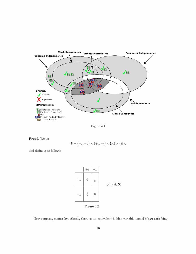
Figure 4.1

Proof. We letΨ = +a,−a × +b,−b × A × B,

and define q as follows:

+b −b

+a 0 12

−a 12 0

q(·, ·|A,B)

Figure 4.2

Now suppose, contra hypothesis, there is an equivalent hidden-variable model (Ω, p) satisfying

16

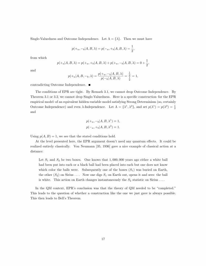
Single-Valuedness and Outcome Independence. Let Λ = λ. Then we must have

p(+a,−b|A,B, λ) = p(−a,+b|A,B, λ) =12,

from whichp(+a|A,B, λ) = p(+a,+b|A,B, λ) + p(+a,−b|A,B, λ) = 0 +

12,

and

p(+a|A,B,−b, λ) =p(+a,−b|A,B, λ)p(−b|A,B, λ)

=1212

= 1,

contradicting Outcome Independence.

The conditions of EPR are tight. By Remark 3.1, we cannot drop Outcome Independence. ByTheorem 3.1 or 3.2, we cannot drop Single-Valuedness. Here is a specific construction–for the EPRempirical model–of an equivalent hidden-variable model satisfying Strong Determinism (so, certainlyOutcome Independence) and even λ-Independence. Let Λ = λ1, λ2, and set p(λ1) = p(λ2) = 1

2

and

p(+a,−b|A,B, λ1) = 1,

p(−a,+b|A,B, λ2) = 1.

Using p(A,B) = 1, we see that the stated conditions hold.At the level presented here, the EPR argument doesn’t need any quantum effects. It could be

realized entirely classically. Von Neumann [35, 1936] gave a nice example of classical action at adistance:

Let S1 and S2 be two boxes. One knows that 1, 000, 000 years ago either a white ballhad been put into each or a black ball had been placed into each but one does not knowwhich color the balls were. Subsequently one of the boxes (S1) was buried on Earth,the other (S2) on Sirius . . . . Now one digs S1 on Earth out, opens it and sees: the ballis white. This action on Earth changes instantaneously the S2 statistic on Sirius . . . .

In the QM context, EPR’s conclusion was that the theory of QM needed to be “completed.”This leads to the question of whether a construction like the one we just gave is always possible.This then leads to Bell’s Theorem.

17

5 Bell

Bell’s Theorem adds crosses to Figure 4.1, as in Figure 5.1.

Figure 5.1

Once more, our formulation is in probability terms alone. In the Bell experiment, Ann (resp. Bob)can make measurements of spin on her (resp. his) entangled particle in three directions. For eachmeasurement, the only possible outcome is positive or negative spin. If the measurements aremade in the same direction, the results will be anti-correlated (Figure 5.2). Figure 5.3 givesthe probabilities of the different outcomes of the measurements, when these are made in differentdirections. The probabilities in Figure 5.3 are essentially quantum-mechanical.

Theorem 5.1 (Bell [2, 1964]) There is an empirical model (Ψ, q) for which there is no equivalenthidden-variable model (Ω, p) which satisfies λ-Independence, Parameter Independence, and OutcomeIndependence.

Another phrasing (using Proposition 2.1): There is no equivalent hidden-variable model whichsatisfies λ-Independence and Locality.

Proof. We letΨ = +a,−a × +b,−b × A1, A2, A3 × B1, B2, B3,

and define q as in Figures 5.2 and 5.3, with q(Ai, Bj) = 19 for all i, j.

18

+b −b

+a 0 12

−a 12 0

q(·, ·|Ai, Bi)

Figure 5.2

+b −b

+a38

18

−a 18

38

q(·, ·|Ai, Bj) for j 6= i

Figure 5.3

Now suppose, contra hypothesis, there is an equivalent hidden-variable model (Ω, p) satisfyingλ-Independence, Parameter Independence, and Outcome Independence.

Fix an i. By assumption, p(Ai, Bi) > 0, since q(Ai, Bi) > 0. Using Figure 5.2, we have

0 = q(+a,+b|Ai, Bi) =∑

λ:p(Ai,Bi,λ)>0

p(+a,+b|Ai, Bi, λ)p(λ|Ai, Bi) =

∑λ:p(Ai,Bi,λ)>0

p(+a,+b|Ai, Bi, λ)p(λ) =

∑λ:p(Ai,Bi,λ)>0

p(+a|Ai, λ)p(+b|Bi, λ)p(λ),

where the second line uses λ-Independence and the third line uses Parameter Independence, OutcomeIndependence, and Proposition 2.1. Using p(Ai, Bi) > 0 and λ-Independence again, we havep(Ai, Bi, λ) > 0 if and only if p(λ) > 0. Let M = λ : p(λ) > 0. Then,

p(+a|Ai, λ)× p(+b|Bi, λ) = 0 (5.1)

whenever λ ∈M .

19

A similar argument using q(−a,−b|Ai, Bi) = 0 establishes

p(−a|Ai, λ)× p(−b|Bi, λ) = 0 (5.2)

whenever λ ∈M .Using (5.1) and (5.2), we see that for each i, there are disjoint sets Ki, Li ⊆ Λ, with Ki∪Li = M ,

such thatp(+a|Ai, λ) = 1 and p(−b|Bi, λ) = 1 when λ ∈ Ki,

p(−a|Bi, λ) = 1 and p(+b|Bi, λ) = 1 when λ ∈ Li.(5.3)

Similar to above, observe that

q(+a,+b|Ai, Bj) =∑M

p(+a|Ai, λ)p(+b|Bj , λ)p(λ). (5.4)

Using (5.3) (for i and j) in (5.4) we get

q(+a,+b|Ai, Bj) = p(Ki ∩ Lj).

A parallel argument yields

q(−a,−b|Ai, Bj) = p(Li ∩Kj).

Now use Figure 5.3 to get

p(Ki ∩ Lj) + p(Li ∩Kj) =34

(5.5)

whenever i 6= j.

Figure 5.4

20

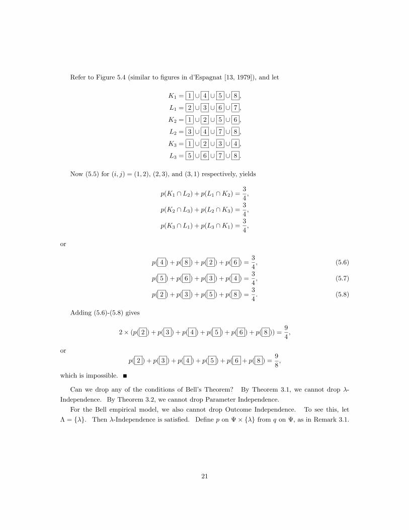
Refer to Figure 5.4 (similar to figures in d’Espagnat [13, 1979]), and let

K1 = 1 ∪ 4 ∪ 5 ∪ 8 ,

L1 = 2 ∪ 3 ∪ 6 ∪ 7 ,

K2 = 1 ∪ 2 ∪ 5 ∪ 6 ,

L2 = 3 ∪ 4 ∪ 7 ∪ 8 ,

K3 = 1 ∪ 2 ∪ 3 ∪ 4 ,

L3 = 5 ∪ 6 ∪ 7 ∪ 8 .

Now (5.5) for (i, j) = (1, 2), (2, 3), and (3, 1) respectively, yields

p(K1 ∩ L2) + p(L1 ∩K2) =34,

p(K2 ∩ L3) + p(L2 ∩K3) =34,

p(K3 ∩ L1) + p(L3 ∩K1) =34,

or

p( 4 ) + p( 8 ) + p( 2 ) + p( 6 ) =34, (5.6)

p( 5 ) + p( 6 ) + p( 3 ) + p( 4 ) =34, (5.7)

p( 2 ) + p( 3 ) + p( 5 ) + p( 8 ) =34. (5.8)

Adding (5.6)-(5.8) gives

2× (p( 2 ) + p( 3 ) + p( 4 ) + p( 5 ) + p( 6 ) + p( 8 )) =94,

orp( 2 ) + p( 3 ) + p( 4 ) + p( 5 ) + p( 6 + p( 8 ) =

98,

which is impossible.

Can we drop any of the conditions of Bell’s Theorem? By Theorem 3.1, we cannot drop λ-Independence. By Theorem 3.2, we cannot drop Parameter Independence.

For the Bell empirical model, we also cannot drop Outcome Independence. To see this, letΛ = λ. Then λ-Independence is satisfied. Define p on Ψ× λ from q on Ψ, as in Remark 3.1.

21

We then have

p(+a|Ai, Bi, λ) = q(+a|Ai, Bi) =12

= q(+a|Ai, Bj) = p(+a|Ai, Bj , λ),

p(+b|Ai, Bi, λ) = q(+b|Ai, Bi) =12

= q(+b|Aj , Bi) = p(+b|Aj , Bi, λ),

so that Parameter Independence is satisfied. Of course, Outcome Independence fails, as it must.For example:

p(+a|−b, Ai, Bi, λ) = 1 6= 12

= p(+a|Ai, Bi, λ).

By contrast, the Kochen-Specker Theorem produces an impossibility even without OutcomeIndependence.

6 Kochen-Specker

The Kochen-Specker [24, 1967] no-go result adds crosses to Figure 5.1, to give a complete picture asin Figure 1.1.

At the physical level, the Kochen-Specker experiment differs from those in the past two sectionsin considering measurements on only one particle. There are many presentations of Kochen-Specker,of course. We follow Cabello, Estebaranz, and Garcıa-Alcaine [8, 1996], a simple treatment whichresults in the 4 × 9 array of Table 6.1. For various tuples of four orthogonal directions in 4-space(from a total of 18 directions), we ask whether or not the particle has spin in each of these directions.In each case, the answer will be that we get three directions without spin and only one directionwith spin.

To state Kochen-Specker in our probabilistic framework, we will need to adapt the concept ofexchangeability from probability theory (de Finetti [11, 1937], [12, 1972]). To give our definition,we consider the special case where the spaces of possible measurements are all the same, as are thespaces of possible outcomes:

A, . . . = B, . . . = · · · = X1, X2, . . . , Xm,

a, . . . = b, . . . = · · · = x1, x2, . . . , xn,

for integers m,n. We will consider a permutation map π:

(A,B, . . .) 7→ (π(A), π(B), . . .),

(a, b, . . .) 7→ (π(a), π(b), . . .).

Note that we use π twice (despite the different domains), because we want to consider the samepermutation on the two sequences.

22

Definition 6.1 An empirical model (Ψ, q) satisfies Exchangeability if for any indices i1, i2, . . . ∈1, 2, . . . ,m and j1, j2, . . . ∈ 1, 2, . . . , n,

q(A = Xi1 , B = Xi2 , . . .) > 0 if and only if q(π(A) = Xi1 , π(B) = Xi2 , . . .) > 0,

for any permutation π, and when both are non-zero,

q(a = xj1 , b = xj2 , . . . |A = Xi1 , B = Xi2 , . . .) =

q(π(a) = xj1 , π(b) = xj2 , . . . |π(A) = Xi1 , π(B) = Xi2 , . . .).

In words, the requirement is that if we swap any number of measurements, then, as long as weswap the outcomes in the same way, the overall probability is unchanged. Thus, let q be the prob-ability that Ann gets the outcome xj1 and Bob gets the outcome xj2 , if Ann performs measurementXi1 on her particle and Bob performs measurement Xi2 on his particle. Let q′ be the probabilitythat Ann gets the outcome xj2 and Bob gets the outcome xj1 , if Ann performs measurement Xi2 onher particle and Bob performs measurement Xi1 on his particle. Exchangeability says that q′ = q.Likewise, for several measurements on a single particle. This is similar to exchangeability a la deFinetti, though with a conditioning component.

Exchangeability might come from physical arguments. For example, the Bell model (Figures 5.2and 5.3) satisfies Exchangeability. (This reflects the underlying physical fact that only the anglebetween the two measurements matters.)

Theorem 6.1 (Kochen-Specker [24, 1967]) There is an empirical model (Ψ, q) for which thereis no equivalent hidden-variable model that satisfies λ-Independence and Parameter Independence.

Kochen-Specker demonstrated the existence of a QM model that fails Non-Contextuality: Whetheror not their particle has spin in a certain direction is dependent on which other directions are alsomeasured. The property of spin for such a particle does not stand alone. As the proof makes clear,Theorem 6.1 is really a corollary to their result.

Proof. Consider an empirical model where

A, . . . = B, . . . = C, . . . = D, . . . = E1, E2, . . . , E18,

a, . . . = b, . . . = c, . . . = d, . . . = 0, 1.

Exchangeability is assumed to hold, and q assigns positive probability to each of the following ninetuples of measurement settings. (The table is from Cabello, Estebaranz, and Garcıa-Alcaine [8,1996], also presented in Held [22, 2000].)

23

A E1 E1 E8 E8 E2 E9 E16 E16 E17

B E2 E5 E9 E11 E5 E11 E17 E18 E18

C E3 E6 E3 E7 E13 E14 E4 E6 E13

D E4 E7 E10 E12 E14 E15 E10 E12 E15

Table 6.1

Finally, for any column, the empirical model has the property that precisely one of the followingholds:

q(1, 0, 0, 0|Ei1 , Ei2 , Ei3 , Ei4) = 1, (6.1)

q(0, 1, 0, 0|Ei1 , Ei2 , Ei3 , Ei4) = 1, (6.2)

q(0, 0, 1, 0|Ei1 , Ei2 , Ei3 , Ei4) = 1, (6.3)

q(0, 0, 0, 1|Ei1 , Ei2 , Ei3 , Ei4) = 1. (6.4)

Now suppose, contra hypothesis, that there is an equivalent hidden-variable model satisfyingλ-Independence and Parameter Independence. By Proposition 2.2, the above empirical model thensatisfies Non-Contextuality.

Next, take, say, the first column. If

q(0, 1, 0, 0|E1, E2, E3, E4) = 1, (6.5)

then certainlyq(b = 1|E1, E2, E3, E4) = 1.

Since (E2, E5, E13, E14) is non-null, so is (E5, E2, E13, E14), by Exchangeability. Using Non-Contextuality, we therefore have

q(b = 1|E5, E2, E13, E14) = 1,

from which, by Exchangeability again,

q(a = 1|E2, E5, E13, E14) = 1.

Now use (6.1)-(6.4) to get

q(1, 0, 0, 0|E2, E5, E13, E14) = 1, (6.6)

which tells us about the fifth column.

24

We therefore get a coloring problem: We try to color precisely one entry in each column–corresponding to the measurement that yields a 1. For example, suppose we color the entry E2 inthe first column–corresponding to (6.5). Then (6.6) tells us that we must color the entry E2 in thefifth column. However, this is impossible. Each Ei appears an even number of times in Table 6.1,and there is an odd number of columns. Thus, the table cannot be colored.

7 Other No-Go Theorems

There are many important papers on the no-go question not touched upon here. These includeGreenberger, Horne, and Zeilinger [20, 1989], Szabo and Fine [31, 2002], Peres [28, 1990], [29, 1991],Fine [17, 1982], [18, 1982], and Mermin [25, 1990], [26, 1993]. Again, our purpose is not to surveythe literature. Rather, it is to give a complete picture of Figure 1.1 and all its 21 regions. As Figure6.1 shows, just the three basic no-go theorems are needed for the six properties that we present.

The absence of Gleason’s Theorem ([19, 1957]) from our paper is a consequence of our choicenot to impose any structure on our spaces (refer back to Footnote 2). In particular, we do notwork in Hilbert space. Of course, Gleason’s Theorem immediately implies the existence of theKochen-Specker QM model (which we used in our Theorem 6.1).

The recent no-go theorem of Conway and Kochen [10, 2006] generalizes Kochen-Specker byrelaxing Parameter Independence. Consider a two-particle system. The requirement is that,conditional on the value of the hidden variable, the outcome of any particular measurement Annmakes on her particle may depend (probabilistically) on the other measurements she makes but noton the measurements Bob makes on his particle. We could accommodate this result by adding aseventh property–a generalized parameter independence–to our six, but refrain from pursuing thisextension here.

Finally, we note the connection to Bohmian mechanics (Bohm [6, 1952]). Durr-Goldstein-Zanghı[15, 2004, p.993] explain: “In Bohmian mechanics the result obtained at one place at any given timewill in fact depend upon the choice of measurement simultaneously performed at the other place.”Indeed, Theorem 3.2 says that provided one is prepared to give up Parameter Independence, onecan reproduce any empirical model–under λ-Independence and Weak Determinism. Theorem 3.1says that if one is prepared to give up λ-Independence, one can get even Strong Determinism. Ina sense, then, these results ‘predict’ the possibility of Bohmian mechanics–though not its specificcontent, of course.

25

References

[1] Belifante, F., A Survey of Hidden-Variable Theories, Pergamon, 1973.

[2] Bell, J., “On the Einstein-Podolsky-Rosen Paradox,” Physics, 1, 1964, 195-200. Reprinted in[4, 1987, pp.14-21].

[3] Bell, J., “Introduction to the Hidden-Variable Question,” in Foundations of Quantum Mechan-ics, Proceedings of the International School of Physics ‘Enrico Fermi’, course IL, AcademicPress, 1971, 171-81. Reprinted in [4, 1987, pp.29-39].

[4] Bell, J., Speakable and Unspeakable in Quantum Mechanics, Cambridge University Press, 1987.

[5] Bohm, D., Quantum Theory, Prentice-Hall, 1951.

[6] Bohm, D., “A Suggested Interpretation of the Quantum Theory in Terms of ‘Hidden’ Variables,I and II,” Physical Review, 85, 1952, 166-193.

[7] Bub, J., Interpreting the Quantum World, Cambridge University Press, 1997.

[8] Cabello, A., J. Estebaranz, and G. Garcıa-Alcaine, “Bell-Kochen-Specker Theorem: A Proofwith 18 Vectors,” Physics Letters A, 212, 1996, 183-187.

[9] Chung, K.L., A Course in Probability Theory, 2nd edition, Academic Press, 1974.

[10] Conway, J., and S. Kochen, “The Free Will Theorem,” 2006. At http://arXiv.org/abs/quant-ph/0604079.

[11] de Finetti, B., “La Prevision: Ses Lois Logiques, Ses Sources Subjectives”, Annales de l’InstitutHenri Poincare, 7, 1937, 1-68. (Translated as “Foresight: Its Logical Laws, Its SubjectiveSources,” in Kyburg, H., and H. Smokler (eds.), Studies in Subjective Probability, Wiley, 1964,53-118.)

[12] de Finetti, B., Probability, Induction, and Statistics, Wiley, 1972.

[13] d’Espagnat, B., “The Quantum Theory and Reality,” Scientific American, November 1979,158-181.

[14] Dickson, W.M., Quantum Chance and Non-Locality: Probability and Non-Locality in the Inter-pretations of Quantum Mechanics, Cambridge University Press, 2005.

[15] Durr, D., S. Goldstein, and N. Zanghı, “Quantum Equilibrium and the Role of Operators asObservables in Quantum Theory,” Journal of Statistical Physics, 116, 2004, 959-1055.

[16] Einstein, A., B. Podolsky, and N. Rosen, “Can Quantum-Mechanical Description of PhysicalReality be Considered Complete?” Physical Review, 47, 1935, 770-780.

26

[17] Fine, A., “Hidden Variables, Joint Probability, and the Bell Inequalities,” Physical ReviewLetters, 48, 1982, 291-295.

[18] Fine, A., “Joint Distributions, Quantum Correlations, and Commuting Observables,” Journalof Mathematical Physics, 23, 1982, 1306–1310.

[19] Gleason, A., “Measures on Closed Sub-Spaces of Hilbert Spaces,” Journal of Mathematics andMechanics, 6, 1957, 885-893.

[20] Greenberger, D., M. Horne, and A. Zeilinger, “Going Beyond Bell’s Theorem,” in M. Kafatos(ed.), Bell’s Theorem, Quantum Theory, and Conceptions of the Universe, Kluwer, 1989, 73–76.

[21] Gudder, S., Quantum Probability, Academic Press, 1988.

[22] Held, C., “The Kochen-Specker Theorem,” 2000. At http://plato.stanford.edu/entries/kochen-specker.

[23] Jarrett, J., “On the Physical Significance of the Locality Conditions in the Bell Arguments,”Nous, 18, 1984, 569-589.

[24] Kochen, S., and E. Specker, “The Problem of Hidden Variables in Quantum Mechanics,” Journalof Mathematics and Mechanics, 17, 1967, 59-87.

[25] Mermin, N.D., “Simple Unified Form for the Major No-Hidden-Variables Theorems, ”PhysicalReview Letters, 65, 1990, 3373–3376.

[26] Mermin, N.D., “Hidden Variables and the Two Theorems of John Bell,”Reviews of ModernPhysics, 65, 1993, 803-815.

[27] Norsen, T., “EPR and Bell Locality,” 2004. At http://www.arxiv.org/abs/quant-ph/0408105.

[28] Peres, A.,“Incompatible Results of Quantum Measurements,”Physics Letters A, 151, 1990, 107–108.

[29] Peres, A.,“Two Simple Proofs of the Kochen-Specker Theorem,”Journal of Physics A, 24, 1991,L175–L178.

[30] Shimony, A., “Events and Processes in the Quantum World,” in Penrose, R., and C. Isham(eds.), Quantum Concepts in Space and Time, Oxford University Press, 1986, 182-203.

[31] Szabo, L., and A. Fine, “A Local Hidden Variable Theory for the GHZ Experiment,” PhysicsLetters, A295, 1997, 229–240.

[32] Teufel, S., K. Berndl, D. Durr, S. Goldstein, and N. Zanghı, “Locality and Causality in HiddenVariables Models of Quantum Theory,” Physical Review A, 56, 1997, 1217-1227.

27

[33] van Fraassen, B., Quantum Mechanics: An Empiricist View, The Clarendon Press, 1991.

[34] von Neumann, J., Mathematische Grundlagen der Quantenmechanik, Springer-Verlag, 1932.(Translated as Mathematical Foundations of Quantum Mechanics, Princeton University Press,1955.)

[35] von Neumann, J., letter to E. Schrodinger, in Redei, M. (ed.), John von Neumann: SelectedLetters, History of Mathematics Volume 27, American Mathematical Society/London Mathe-matical Society, 2005, 211-213.

[36] Werner, R., and M. Wolf, “Bell Inequalities and Entanglement,” Quantum Information & Com-putation, 1(3), 2001, 1-25.

28