A class of Petri nets for modelingand analyzing business processesW.M.P. van der AalstDepartment of Mathematics and Computing Science, Eindhoven University of Technol-ogy,P.O. Box 513, NL-5600 MB, Eindhoven, The Netherlands, telephone: -31 40 474295, e-mail: wsinwa@win.tue.nl

More and more firms are marching to the drumbeat of Business Process Reengineering(BPR) and Workflow Management (WFM). This trend exposes the need for techniques forthe construction and analysis of business procedures. In this paper we focus on a class ofPetri nets suitable for the representation, validation and verification of these procedures.We will show that the correctness of a procedure represented by such a Petri net canbe verified in polynomial time. Based on this result we provide a comprehensive set oftransformation rules which can be used to construct and modify correct procedures.

Keywords: Petri nets; free-choice Petri nets; Business Process Reengineering; WorkflowManagement; analysis of Petri nets.

1 Introduction

The flourish of trumpets surrounding the terms Business Process Reengineering(BPR) and Workflow Management (WFM) signifies the focus on business pro-cesses. Workflow management systems allow for the continuous improvement ofthe business processes at hand. Business Process Reengineering efforts are aimedat dramatic improvements by a radical redesign of the business processes. Today’scompetitive organizations are reshaping to the needs of their primary business pro-cesses. Therefore, it is important to furnish business processes with a theoreticalbasis, analysis techniques and tools. In this paper we focus on modeling and ana-lyzing the procedures underlying these business processes.

Business processes are centered round procedures. A procedure is the methodof operation used by a business process to process cases. Examples of cases areorders, claims, travel expenses, tax declarations, etc. The procedure specifies theset of tasks required to process these cases successfully. Moreover, the proce-dure specifies the order in which these tasks have to be executed. The goal of

1

a procedure is to handle cases efficiently and properly. To achieve this goal, theprocedure should be tuned to the ever changing environment of the business pro-cess. WFM and BPR are the keywords which herald a new era of frequent and/orradical changes of existing procedures.

In this paper we focus on the use of Petri nets ([17, 18, 19]) as a tool for the rep-resentation, validation and verification of business procedures. It is not difficult tomap a procedure onto a Petri net. As it turns out, we can even restrict ourselves to asubclass of Petri nets. Representatives of this class are called Business-Procedurenets (BP-nets). A BP-net is a free-choice Petri net (Desel and Esparza [12]) withtwo special places: i and o. These places are used to mark the begin and the endof a procedure, see figure 1. The tasks are modeled by transitions and the partialordering of tasks is modeled by places connecting these transitions.

WF-neti o

Figure 1: A procedure modeled by a BP-net.

The processing of a case starts the moment we put a token in place i and terminatesthe moment a token appears in place o. One of the main properties a properprocedure should satisfy is the following:

For any case, the procedure will terminate eventually and the momentthe procedure terminates there is a token in place o and all the otherplaces are empty.

This property is called the soundness property. In this paper we present a tech-nique to verify this property in polynomial time. This technique is based on therich theory developed for free-choice Petri nets (cf. Best [6], Desel and Esparza[12]).

BP-nets have some interesting properties. For example, it turns out that a BP-net is

2

sound if and only if a slightly modified version of this net is live and bounded! Wewill use this property to show that there is a comprehensive set of transformationrules which preserve soundness. These transformation rules show how a soundprocedure can be transformed into another sound procedure. In the context ofWFM and BPR, where procedures have to be modified frequently or radically,these transformation rules are useful.

The remainder of this paper is organized as follows. In Section 2 we introducesome of the basic notations for Petri nets. Section 3 deals with BP-nets. In thissection we also define the soundness property. In Section 4 we present a techniqueto verify the soundness property. Some new results for free-choice Petri netsare presented in Section 5. These results are used to prove that some extendedsoundness property holds for sound BP-nets. A set of transformation rules thatpreserve soundness is presented in Section 6.

2 Petri nets

Historically speaking, Petri nets originate from the early work of Carl Adam Petri([19]). Since then the use and study of Petri nets has increased considerably. Fora review of the history of Petri nets and an extensive bibliography the reader isreferred to Murata [17].

The classical Petri net is a directed bipartite graph with two node types calledplaces and transitions. The nodes are connected via directed arcs. Connectionsbetween two nodes of the same type are not allowed. Places are represented bycircles and transitions by rectangles.

Definition 1 (Petri net) A Petri net is a triplet (P, T , F):

- P is a finite set of places,

- T is a finite set of transitions (P ∩ T = ∅),

- F ⊆ (P × T ) ∪ (T × P) is a set of arcs (flow relation)

A place p is called an input place of a transition t iff there exists a directed arcfrom p to t . Place p is called an output place of transition t iff there exists adirected arc from t to p. We use •t to denote the set of input places for a transi-tion t . The notations t•, •p and p• have similar meanings, e.g. p• is the set oftransitions sharing p as an input place.

Places may contain zero or more tokens, drawn as black dots. The state, often

3

referred to as marking, is the distribution of tokens over places. We will representa state as follows: 1p1 + 2p2 + 1p3 + 0p4 is the state with one token in place p1,two tokens in p2, one token in p3 and no tokens in p4. We can also represent thisstate as follows: p1 + 2p2 + p3.

The number of tokens may change during the execution of the net. Transitions arethe active components in a Petri net: they change the state of the net according tothe following firing rule:

(1) A transition t is said to be enabled iff each input place p of t contains atleast one token.

(2) An enabled transition may fire. If transition t fires, then t consumes onetoken from each input place p of t and produces one token for each outputplace p of t .

Given a Petri net (P, T , F) and an initial state M1, we have the following nota-tions:

- M1t→ M2: transition t is enabled in state M1 and firing t in M1 results in

state M2

- M1 → M2: there is a transition t such that M1t→ M2

- M1σ→ Mn : the firing sequence σ = t1t2t3 . . . tn−1 leads from state M1 to

state Mn , i.e. M1t1→ M2

t2→ ...tn−1→ Mn

- M1∗→ Mn: there is a firing sequence which leads from M1 to Mn

A state Mn is called reachable from M1 (notation M1∗→ Mn) iff there is a firing

sequence σ = t1t2 . . . tn−1 such that M1t1→ M2

t2→ ...tn−1→ Mn .

Let σ = t1t2 . . . tn be a firing sequence of length n. For k such that 1 ≤ k ≤ n, wehave the following notations:

- σ(k) = tk

- σ k = t1t2 . . . tk

A state M is a dead state iff no transition is enabled in M . For a state M and aplace p, we use M(p) to denote the number of tokens in p in state M . For twostates M and N , M ≤ N iff for each place p: M(p) ≤ N (p).

Let us define some properties.

4

Definition 2 (Conservative) A Petri net PN is conservative iff there is a positiveinteger w(p) for every place p such that, given an arbitrary initial state M, theweighted sum of tokens is constant for every reachable state M ′.

Definition 3 (Live) A Petri net (PN , M) is live iff, for every reachable state M ′and every transition t there is a state M ′′ reachable from M ′ which enables t .

Definition 4 (Bounded) A Petri net (PN , M) is bounded iff, for every reachablestate and every place p the number of tokens in p is bounded.

Definition 5 (Strongly connected) A Petri net is strongly connected iff, for everytwo places (transitions) x and y, there is a directed path leading from x to y.

In this paper we use a restricted class of Petri nets for modeling and analyzingbusiness procedures. As we will see in Section 3, it suffices to consider Petri netssatisfying the so-called free-choice property.

Definition 6 (Free-choice) A Petri net is a free-choice Petri net iff, for every twoplaces p1 and p2 either (p1 • ∩ p2•) = ∅ or p1• = p2•.

Free-choice Petri nets have been studied extensively (cf. Best [6], Desel and Es-parza [12, 11, 13], Hack [14]) because they seem to be a good compromise be-tween expressive power and analyzability. It is a class of Petri nets for whichstrong theoretical results and efficient analysis techniques exist.

For reasons of simplicity we only consider classical Petri nets. (As a matter of factonly free-choice Petri nets.) However, the results in this paper can be extendedto high-level Petri nets, i.e. Petri nets extended with (i) ‘color’ (tokens have avalue), (ii) ‘time’ (it is possible to model durations) and (iii) ‘hierarchy’ (a net maybe composed of subnets). In fact we are planning to incorporate the techniquespresented in this paper in the software package ExSpect ([10]). ExSpect is a toolbased on high-level Petri nets which has been used to model and analyze manyindustrial systems ([3]). For more details about the model ExSpect is based on thereader is referred to [1, 2, 15]. As a matter of fact, it is a model quite similar tothe CPN-model by Jensen (cf. [16]).

3 BP-nets

3.1 What is a procedure?

A common feature of Workflow Management and Business Process Reengineer-ing is the focus on business processes. Workflow management systems are cen-tered round the definition of a business process, often referred to as workflow.

5

Business Process Reengineering involves the explicit reconsideration and redesignof business processes.The objective of a business process is the processing of cases (e.g. claims, orders,travel expenses). To completely define a business process we have to specify twothings ([5, 4]):

(i) A procedure: a partially ordered set of tasks.

(ii) An allocation of resources to tasks.

The procedure specifies the set of tasks required to process cases successfully.(Synonyms for task are process activity, step and node.) Moreover, the proce-dure specifies the order in which these tasks have to be executed. (Tasks may beoptional or mandatory and are executed in parallel or sequential order.) The allo-cation of resources to tasks is required to decide who is going to execute a specifictask for a specific case. Each resource (e.g. a secretary) is able to perform certainfunctions (e.g. typing a letter) and each task requires certain functions. A resourcemay be allocated to a task, if the resource provides the required functions.In this paper we concentrate on modeling (business) procedures, i.e. we abstractfrom the resources required to execute these procedures.To illustrate the term (business) procedure we will use the following example.Consider an automobile insurance company. The business process process claimtakes care of the processing of claims related to car damage. Each claim corre-sponds to a case to be handled by process claim. The business procedure thatis used to handle these cases can be described as follows. There are four tasks:check insurance, contact garage, pay damage and send letter. The tasks check insuranceand contact garage may be executed in any order to determine whether the claimis justified. If the claim is justified, the damage is paid (task pay damage). Other-wise a ‘letter of rejection’ is sent to the claimant (task send letter).

3.2 Modeling a procedure

We use Petri nets for modeling and analyzing business procedures. Basically, aprocedure is a partially ordered set of tasks. Therefore, it is quite easy to map aprocedure onto a Petri net. Tasks are modeled by transitions and precedence re-lations are modeled by places. Consider for example the business procedure pro-cess claim, see figure 2. The tasks check insurance, contact garage, pay damageand send letter are modeled by transitions. Since the two tasks check insuranceand contact garage may be executed in parallel, there are two additional transi-tions: fork and join. The places p1, p2, p3, p4 and p5 are used to route a casethrough the procedure in a proper manner.

6

fork

i

p1 p2

contact_garage

join

p3 p4

p5

send_letter

o

pay_damage

check_insurance

Figure 2: The business procedure process claim.

Cases are processed independently, i.e. a task executed for some case cannot influ-ence a task executed for another task. Nevertheless, the throughput time of a casemay increase if there are many other cases competing for the same resources. Inthis paper we abstract from resources: cases do not affect each other in any way.Therefore, it suffices to consider one case at a time (cf. Section 5). The token inplace i in figure 2 corresponds to one case. During the processing of a case theremay be several tokens referring to the same case. (If transition fork fires, thenthere are two tokens, one in p1 and one in p2, referring to the same claim.) Theprocessing of the case is completed if there is a token in place o and there are noother tokens also referring to the same case.

Petri nets which model business procedures have some typical properties. First ofall, they always have two special places i and o, which correspond to the begin-ning and termination of the processing of a case respectively. Place i is a sourceplace and o is a sink place. Secondly, a Petri net which represents a business pro-cedure is always a free-choice Petri net. Thirdly, for each transition t there shouldbe directed path from place i to o via t . A Petri net which satisfies these threerequirements is called a Business-Procedure net (BP-net), see figure 1.

7

Definition 7 (BP-net) A Petri net PN = (P, T , F) is a BP-net (Business-Procedurenet) if and only if:

(i) PN has two special places: i and o. Place i is a source place: •i = ∅.Place o is a sink place: o• = ∅.

(ii) PN is a free-choice Petri net.

(iii) If we add a transition t ∗ to PN which connects place o with i (i.e. •t∗ = {o}and t∗• = {i}), then the resulting Petri net is strongly connected.

The reason for restricting BP-nets to free-choice Petri nets is pragmatic: we sim-ply cannot think of a sensible business procedure which violates the free-choiceproperty (see definition 6). We can model parallelism, sequential routing, con-ditional routing and iteration without violating the free-choice property (cf. Sec-tion 6). The third requirement (the Petri net extended with t ∗ should be stronglyconnected), states that for each transition t there should be directed path fromplace i to o via t . This requirement has been added to avoid ‘dangling tasks’, i.e.tasks which do not contribute to the processing of cases.

It is easy to verify that the Petri net shown in figure 2 is a BP-net.

3.3 Sound procedures

The three requirements stated in definition 7 can be verified statically, i.e. theyonly relate to the structure of the Petri net. There is however a fourth propertywhich should be satisfied:

For any case, the procedure will terminate eventually and the momentthe procedure terminates there is a token in place o and all the otherplaces are empty.

This property is called the soundness property.

Definition 8 (Sound) A procedure modeled by a BP-net PN = (P, T , F) issound if and only if:

(i) For every state M reachable from state i , there exists a firing sequenceleading from state M to state o. Formally:

∀M(i∗→ M) ⇒ (M

∗→ o)

8

(ii) State o is the only state reachable from state i with at least one token inplace o. Formally:

∀M(i∗→ M ∧ M ≥ o) ⇒ (M = o)

Note that the soundness property relates to the dynamics of a BP-net. The firstrequirement in definition 8 states that starting from the initial state (state i), it isalways possible to reach the state with one token in place o (state o). (Note thatthere is an overloading of notation: the symbol i is used to denote both the place iand the state with only one token in place i (see Section 2).) If we assume fairness(i.e. a transition that is enabled infinitely often will fire eventually), then the firstrequirement implies that eventually state o is reached. The second requirementstates that the moment a token is put in place o, all the other places should beempty.

For the BP-net shown in figure 2 it is easy to see that it is sound. However, forcomplex business procedures it is far from trivial to check the soundness property.

4 Analysis of BP-nets

4.1 Introduction

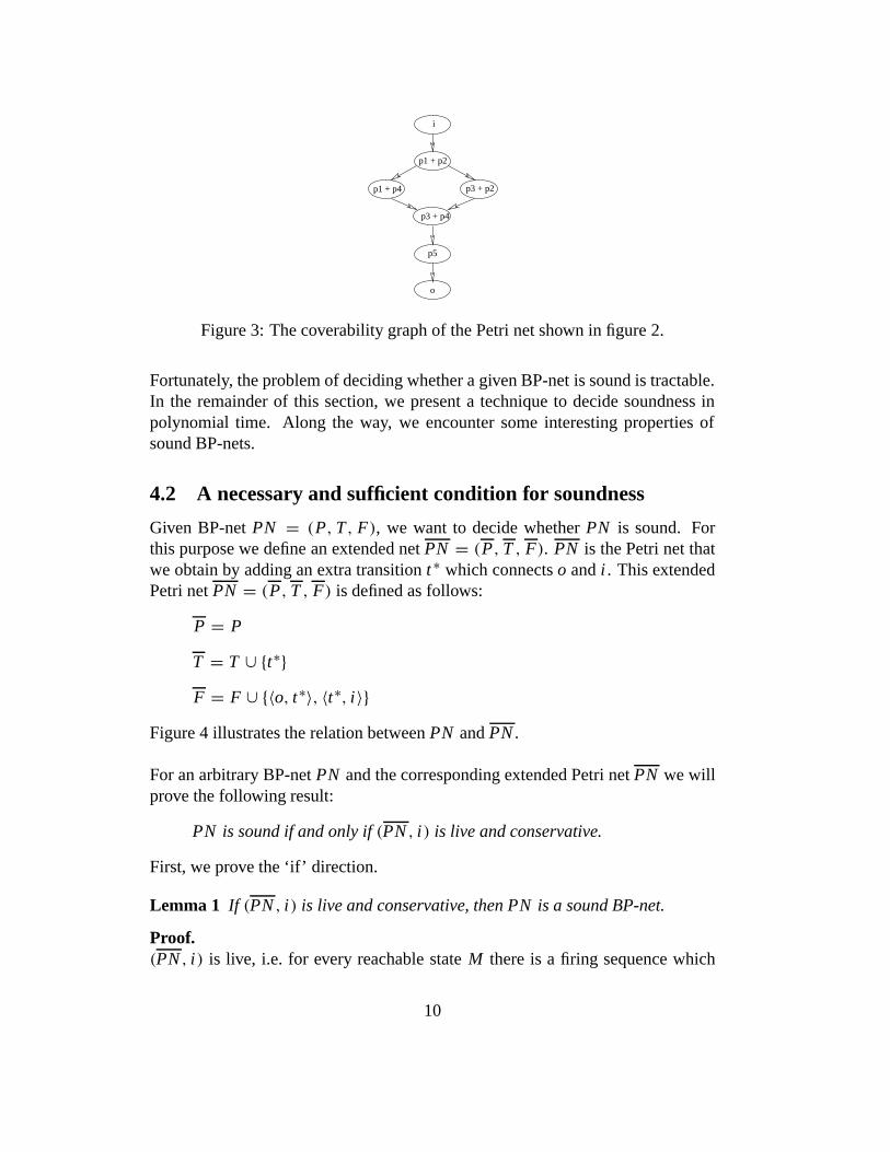
In this section, we focus on analysis techniques that can be used to verify thesoundness property. The soundness property is a property which relates to thedynamics of a BP-net. Therefore, the coverability graph (Peterson [18], Murata[17]) seems to be an obvious technique to check whether the BP-net is sound.Figure 3 shows the coverability graph which corresponds to the Petri net shownin figure 2 (the initial state is i). There are only 6 reachable states, therefore it iseasy to verify the two requirements stated in definition 8.In general the coverability graph can be used to decide whether a BP-net is sound.1

However, for complex procedures, the construction of the coverability graph maybe very time consuming. The complexity of the algorithm to construct the cov-erability graph can be worse than primitive recursive space. Even for free-choicePetri nets the reachability problem is known to be EXPSPACE-hard (cf. Cheng,Esparza and Palsberg [9]). Therefore, any ‘brute-force approach’ to check sound-ness is bound to be intractable.

1In Section 4.2 we show that a sound BP-net is bounded. If the coverability graph has anunbounded state (an ‘ω-state’), then the BP-net is not sound. Otherwise, we can use a simplealgorithm to check the two requirements stated in definition 8.

9

i

p1 + p2

p1 + p4 p3 + p2

o

p5

p3 + p4

Figure 3: The coverability graph of the Petri net shown in figure 2.

Fortunately, the problem of deciding whether a given BP-net is sound is tractable.In the remainder of this section, we present a technique to decide soundness inpolynomial time. Along the way, we encounter some interesting properties ofsound BP-nets.

4.2 A necessary and sufficient condition for soundness

Given BP-net PN = (P, T , F), we want to decide whether PN is sound. Forthis purpose we define an extended net PN = (P, T , F). PN is the Petri net thatwe obtain by adding an extra transition t ∗ which connects o and i . This extendedPetri net PN = (P, T , F) is defined as follows:

P = P

T = T ∪ {t∗}F = F ∪ {〈o, t∗〉, 〈t∗, i〉}

Figure 4 illustrates the relation between PN and PN .

For an arbitrary BP-net PN and the corresponding extended Petri net PN we willprove the following result:

PN is sound if and only if (PN , i) is live and conservative.

First, we prove the ‘if’ direction.

Lemma 1 If (PN , i) is live and conservative, then PN is a sound BP-net.

Proof.(PN , i) is live, i.e. for every reachable state M there is a firing sequence which

10

PN

*

i

t

o

Figure 4: PN = (P, T ∪ {t∗}, F ∪ {〈o, t∗〉, 〈t∗, i〉}).

leads to a state in which t∗ is enabled. Since o is the input place of t ∗, we find thatfor any state M reachable from state i it is possible to reach a state with at leastone token in place o. PN is conservative, therefore there is a semi-positive placeinvariant with a support equal to P . The places i and o have the same positiveweight because t∗ may move a token from o to i . The only state with at least onetoken in place o and reachable from state i is the state o.So if (PN , i) is live and conservative, then PN satisfies the following properties:(i) for every state M reachable from state i , there exists a firing sequence leadingfrom state M to state o and (ii) state o is the only state reachable from state i withat least one token in place o. Hence, PN is a sound BP-net. �

To prove the ‘only if’ direction, we first show that the extended net is bounded.

Lemma 2 If PN is sound, then (PN , i) is bounded.

Proof.Assume that PN is sound and (PN , i) not bounded. Since PN is not boundedthere are two states Mi and M j such that i

∗→ Mi , Mi∗→ M j and M j > Mi .

(See for example the proof that the coverability tree is finite in Peterson [18] (the-orem 4.1).) However, since PN is sound we know that there is a firing sequence σ

such that Miσ→ o. Therefore, there is a state M such that M j

σ→ M and M > o.Hence, it is not possible that PN is both sound and not bounded. So if PN issound, then (PN , i) is bounded.From the fact that PN is sound and (PN , i) is bounded we can deduce that (PN , i)is bounded. If transition t ∗ in PN fires, the net returns to the initial state i . �

Now we can prove that (PN , i) is live and conservative.

11

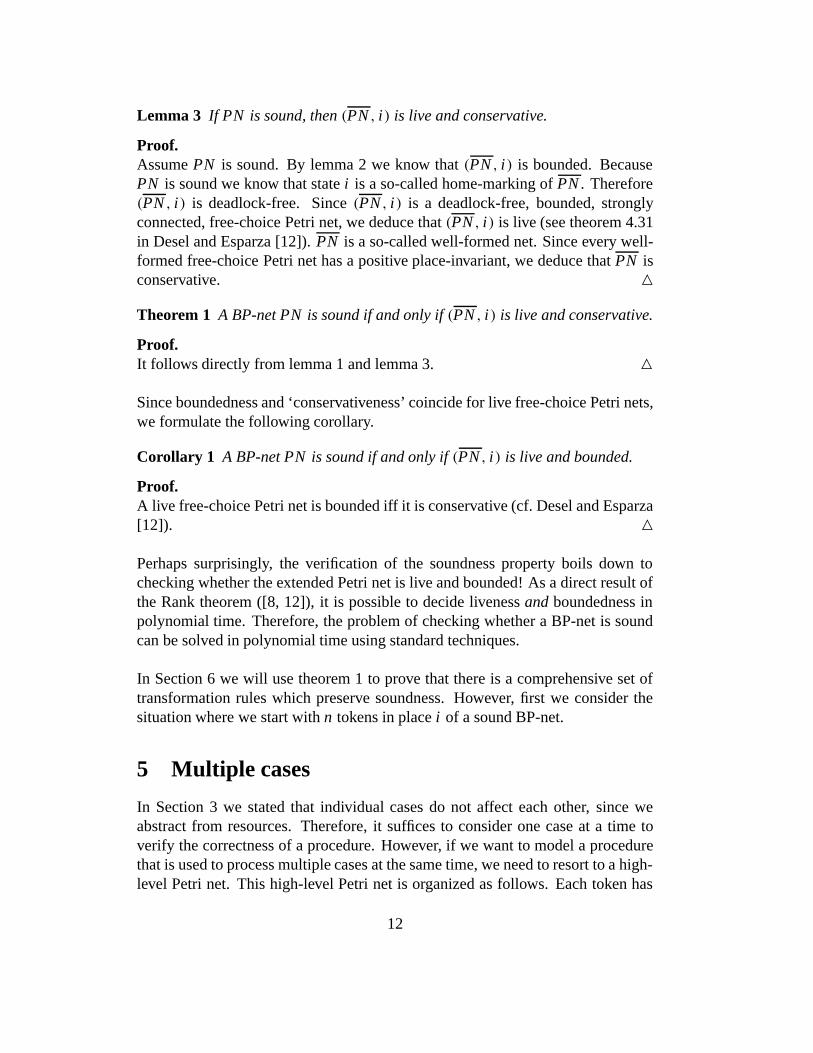
Lemma 3 If PN is sound, then (PN , i) is live and conservative.

Proof.Assume PN is sound. By lemma 2 we know that (PN , i) is bounded. BecausePN is sound we know that state i is a so-called home-marking of PN . Therefore(PN , i) is deadlock-free. Since (PN , i) is a deadlock-free, bounded, stronglyconnected, free-choice Petri net, we deduce that (PN , i) is live (see theorem 4.31in Desel and Esparza [12]). PN is a so-called well-formed net. Since every well-formed free-choice Petri net has a positive place-invariant, we deduce that PN isconservative. �Theorem 1 A BP-net PN is sound if and only if (PN , i) is live and conservative.

Proof.It follows directly from lemma 1 and lemma 3. �

Since boundedness and ‘conservativeness’ coincide for live free-choice Petri nets,we formulate the following corollary.

Corollary 1 A BP-net PN is sound if and only if (PN , i) is live and bounded.

Proof.A live free-choice Petri net is bounded iff it is conservative (cf. Desel and Esparza[12]). �

Perhaps surprisingly, the verification of the soundness property boils down tochecking whether the extended Petri net is live and bounded! As a direct result ofthe Rank theorem ([8, 12]), it is possible to decide liveness and boundedness inpolynomial time. Therefore, the problem of checking whether a BP-net is soundcan be solved in polynomial time using standard techniques.

In Section 6 we will use theorem 1 to prove that there is a comprehensive set oftransformation rules which preserve soundness. However, first we consider thesituation where we start with n tokens in place i of a sound BP-net.

5 Multiple cases

In Section 3 we stated that individual cases do not affect each other, since weabstract from resources. Therefore, it suffices to consider one case at a time toverify the correctness of a procedure. However, if we want to model a procedurethat is used to process multiple cases at the same time, we need to resort to a high-level Petri net. This high-level Petri net is organized as follows. Each token has

12

a value which refers to the case it belongs to and transitions can only consumetokens which belong to the same case. It is easy to see that in this high-level Petrinet individual cases do not affect each other. Nevertheless, it is interesting to seewhat happens if we abstract from color, i.e. we allow multiple indistinguishablecases. In this section we will show that we can extend the soundness propertyfor the situation where there are an arbitrary number of cases. As it turns outthis extended soundness property coincides with the soundness property definedin Section 3.3.

First we prove some preliminary results which hold for any free-choice Petri net.

5.1 Substate-ordering Lemma

One of the fundamental properties of a free-choice Petri net is the fact that it canbe partitioned into clusters.

Definition 9 (Cluster) Let t be a transition in a free-choice Petri net. The clusterof t , denoted by [t], is the set •t ∪ {t ′ ∈ T | • t ′ = •t}. The cluster of a place p,also denoted by [p], is the set p • ∪ {p′ ∈ P | (p′ • ∩ p•) �= ∅}.Note that a place p and a transition t belong to the same cluster (i.e. [p] = [t]) iffp ∈ •t . For free-choice Petri nets, we have the following property. If transition tis enabled, then any transition in [t] is enabled. A cluster c is called enabled iffthe transitions in c are enabled.

The first result we present is the advance lemma. This lemma shows that given afiring sequence it is possible to advance the firing of certain transitions.

Lemma 4 (Advance lemma) Let σ = t1t2 . . . tk be a firing sequence of a free-choice Petri net such that σ leads from state M to state M ′, i.e. M

σ→ M ′. If acluster c is enabled in state M and ti is the first transition in σ such that ti ∈ c,

then Mσ ′→ M ′ with σ ′ = ti t1t2 . . . ti−1ti+1 . . . tk .

Proof.In state M each of the transitions in c is enabled, i.e. transition ti is enabled instate M . The transitions t j with 1 ≤ j < i are not disabled by the advanced firingof ti , because they belong to different clusters. Therefore, the firing sequenceσ ′ = ti t1t2 . . . ti−1ti+1 . . . tk is possible. Since σ ′ is a permutation of σ , we deduce

that Mσ ′→ M ′. �

We use the advance lemma to prove the substate-ordering lemma. The substate-ordering lemma is illustrated in figure 5.

13

N

N’

M

M’

M’+(N-M)

Figure 5: The substate-ordering lemma.

Lemma 5 (Substate-ordering lemma) Let PN be a free-choice Petri net and Nand N ′ states of PN such that N

∗→ N ′ and N ′ is dead. For any substate M of N

(i.e. M ≤ N), there is a dead state M ′ such that M∗→ M ′ and M ′ + (N − M)

∗→N ′.

Proof.Let σ = t1t2 . . . tk be an arbitrary firing sequence leading from N to N ′ (N

σ→ N ′).We use induction upon the length k of σ .If k = 0, then N = N ′. Since N is dead (N = N ′) and M ≤ N , M is also dead.Hence, M ′ = M is a dead state such that M

∗→ M ′ and M ′ + (N − M)∗→ N ′.

Assume k > 0. If M is dead, then for M ′ = M the lemma holds. Therefore, wemay assume that M is not dead. Let ti be the first transition in σ which is enabledin M , i.e. ti is enabled in M and for all 1 ≤ j < i : t j is not enabled in M . Notethat such a transition exists, because M ≤ N , M is not dead and N ′ is dead. Thecluster [ti ] is enabled in N and ti is the first transition in σ which belongs to [ti ].

We can use lemma 4 to prove that Nσ ′→ N ′ with σ ′ = ti t1t2 . . . ti−1ti+1 . . . tk .

Let N1 and M1 be states such that Nti→ N1 and M

ti→ M1. By the inductionhypothesis we can show that there is a dead state M ′ such that M1

∗→ M ′ andM ′ + (N1 − M1)

∗→ N ′. By the definition of N1 and M1 we conclude thatM

∗→ M ′ and M ′ + (N − M)∗→ N ′. �

Note that these results hold for any free-choice Petri net. The substate-orderinglemma will be used to prove theorem 2.

5.2 Sound BP-nets which handle multiple cases

Consider the BP-net shown in figure 6. If we add a transition t∗ which connects oand i , then the resulting net is live and bounded. Therefore, the BP-net shown infigure 6 is sound. If we put one token in place i , then eventually there will be onetoken in o and at the same time all the other places will be empty. What happens ifwe put 10 tokens in place i? Even for the small net shown in figure 6 it is not easy

14

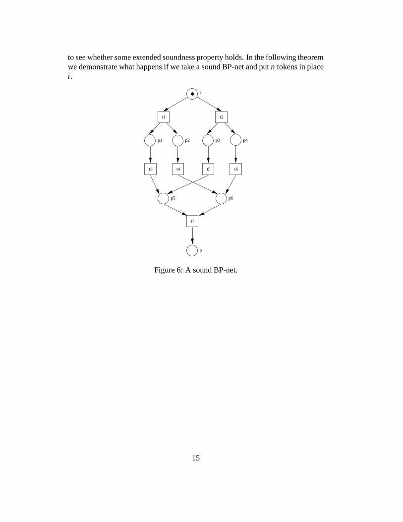
to see whether some extended soundness property holds. In the following theoremwe demonstrate what happens if we take a sound BP-net and put n tokens in placei .

t1 t2

t3 t4 t5 t6

t7

p5 p6

p4p3p2p1

o

i

Figure 6: A sound BP-net.

15

Theorem 2 If PN is sound, then for every n ∈ IN:

(i) For every state M reachable from state ni ,2 there exists a firing sequenceleading from state M to state no. Formally:

∀M(ni∗→ M) ⇒ (M

∗→ no)

(ii) State no is the only state reachable from state ni with at least n tokens inplace o. Formally:

∀M(ni∗→ M ∧ M ≥ no) ⇒ (M = no)

Proof.Assume PN is sound. By theorem 1, we know that (PN , i) is live and conserva-tive. Therefore, PN has a positive place invariant which assigns identical weightsto the places i and o. This invariant also holds for PN . Hence, the only reachablestate with at least n tokens in place o is the state no, i.e. (ii) holds.

Before we prove that (i) holds we prove that for any state M reachable fromstate ni (i.e. ni

∗→ M), it is possible to reach a dead state N ′, i.e. (PN , M) isnot deadlock-free. Suppose that (PN , M) is deadlock-free. Since (PN , M) isbounded, there is some recurrent state X such that M

∗→ X and any infinite fir-ing sequence starting from X will visit X infinitely often. Consider all the firingsequences σ such that X

σ→ X . Let PX be the set of places “affected” by at leastone of these firing sequences. Since PN is a free-choice Petri net, it is easy toverify that PX is a trap. Clearly, the places i and o are not in PX . Therefore, PX isalso a trap of PN . In state ni there are no tokens in trap PX . By using the Homemarking theorem (cf. Best, Desel and Esparza [7]), we deduce that ni is not ahome marking of (PN , ni). However, state i is a home marking of (PN , i) and niis also a home marking of (PN , ni). Based on this contradiction, we deduce that(PN , M) is not deadlock-free.

Remains to prove that for any state M reachable from state ni , there is a firingsequence leading from state M to state no (see (i)). We have just deduced that(PN , M) is not deadlock-free, i.e. given a state M reachable from state ni it ispossible to reach some dead state N ′.It suffices to prove that state N ′ is equal no. We use induction to prove this.

2Note that ni is used to denote the state with n tokens in place i ; no is used to denote the statewith n tokens in place o.

16

• If n = 0 or n = 1, this holds by definition. If n = 0 the only reachable stateis the state without tokens. (This state can be denoted by 0o.) If n = 1, theonly reachable dead state is 1o (see definition 8).

• Assume n > 1. By applying lemma 5 we find that there is a dead state M ′such that i

∗→ M ′ and M ′ + (ni − i)∗→ N ′. Since PN is sound we know

that the only state M ′ such that i∗→ M ′ is the state o, i.e. M ′ = o. Hence,

o + (n − 1)i∗→ N ′. Since o is a sink place (o• = ∅), (n − 1)i

∗→ N ′ − o.The state N ′ − o is also dead. By the induction hypothesis we conclude thatstate N ′ is equal to no.

Hence, (i) also holds. �

This theorem shows that if we extend the soundness property to the situationwhere there are an arbitrary number of tokens in i (in a straightforward manner),then this extended soundness property coincides with the soundness property de-fined in Section 3.3.

17

6 Transformation rules

Workflow Management and Business Process Reengineering are marked by theawareness that procedures should be subject to change. Therefore, it is interestingto investigate which changes preserve soundness.

In our opinion there are eight basic transformation rules (T1a, T1b, T2a, T2b,T3a, T3b, T4a and T4b) which can be used to modify a sound business procedure.These transformation rules are shown in figures 7, 8, 9 and 10 and elucidated inthe sequel.

T1a Task t1 is replaced by two consecutive tasks t2 and t3. This transformationrule corresponds to the division of a task: a complex task is divided into twotasks which are less complicated. (See figure 7.)

i

o

t1

i

o

t2

t3

p

Rule T1a

Rule T1b

Figure 7: Transformation rules: T1a and T1b.

T1b Two consecutive tasks t2 and t3 are replaced by one task t1. This transfor-mation rule is the opposite of T1a and corresponds to the aggregation oftasks. Two tasks are combined into one task. (See figure 7.)

T2a Task t1 is replaced by two conditional tasks t2 and t3. This transformationrule corresponds to the specialization of a task (e.g. handle order) into twomore specialized tasks (e.g. handle small order and handle large order).(See figure 8.)

18

i

o

t1

i

o

Rule T2a

Rule T2b

t2 t3

Figure 8: Transformation rules: T2a and T2b.

T2b Two conditional tasks t2 and t3 are replaced by one task t1. This transfor-mation rule is the opposite of T2a and corresponds to the generalization oftasks. Two rather specific tasks are replaced by one more generic task. (Seefigure 8.)

T3a Task t1 is replaced by two parallel tasks t2 and t3. (See figure 9.) The effectof the execution of t2 and t3 is identical to the effect of the execution of t1.The transitions c1 and c2 represent control activities to fork and join twoparallel threads.

T3b The opposite of transformation rule T3a: two parallel tasks t2 and t3 arereplaced by one task t1. (See figure 9.)

T4a Task t1 is replaced by an iteration of task t2. (See figure 10.) The exe-cution of task t1 (e.g. type letter) corresponds to zero or more executionsof task t2 (e.g. type sentence). The transitions c1 and c2 represent controlactivities that mark the begin and end of a sequence of ‘t2-tasks’. Typicalexamples of situations where iteration is required are quality control andcommunication.

T4b The opposite of transformation rule T4a: the iteration of t2 is replaced bytask t1. (See figure 10.)

19

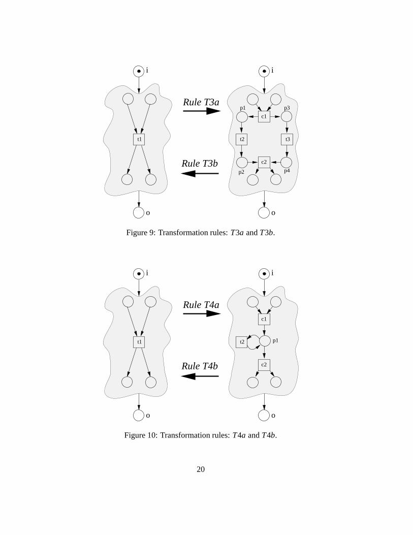
i

o

t1

i

o

t3t2

c2

c1

p2

p1 p3

p4

Rule T3a

Rule T3b

Figure 9: Transformation rules: T3a and T3b.

i

o

t1

i

o

c2

c1

Rule T4a

Rule T4b

p1t2

Figure 10: Transformation rules: T4a and T4b.

20

It is easy to see that if we take a sound BP-net and we apply one of these transfor-mation rules, then the resulting Petri net is still a BP-net. Moreover, the resultingBP-net is also sound.

Theorem 3 The transformation rules T1a, T1b, T2a, T2b, T3a, T3b, T4a andT4b preserve soundness, i.e. if a BP-net is sound, then the BP-net transformed byone of these rules is also sound.

Proof.We use theorem 1 to prove that the transformation rules preserve soundness. As-sume that the net PN is sound. By theorem 1 we know that (PN , i) is live and con-servative. The transformation rule transforms PN into PN ′. PN ′ is the Petri netPN ′ with an extra transition t∗ which connects place o and place i . By theorem 1we also know that PN ′ is sound if and only if (PN ′, i) is live and conservative.(i) (PN ′, i) is liveEach of the transformation rules T1a, T1b, T2a, T2b, T3a, T3b, T4a and T4bpreserves liveness. It is easy to verify this for each transformation rule. Considerthe transformation rules shown in figure 7 and 8. Transition t1 is live if andonly if t2 and t3 are live (i.e. T1a, T1b, T2a and T2b preserve liveness). Thetransformation rules T3a and T3b (see figure 9) also preserve liveness: t1 is liveif and only if c1, c2, t2 and t3 are live. The transformation rules shown in figure 10(i.e. T4a and T4b) also preserve liveness: t1 is live if and only if c1, c2, and t2are live.(ii) PN ′ is conservativePN has a positive place-invariant. It is easy to see that this place-invariant can bemodified such that it is an invariant of PN ′.Hence, PN ′ is sound. �

The eight transformation rules shown in figures 7, 8, 9 and 10 preserve soundness.We can use these basic transformation rules to construct more complex transfor-mation rules. Figure 11 shows two of these rules: T5a and T5b.

T5a Two consecutive tasks are replaced by two parallel tasks.

T5b Two parallel tasks are replaced by two consecutive tasks.

The application of transformation rule T5a corresponds to the application of T1bfollowed by the application of T3a. Transformation rule T5b is a combinationof T3b and T1a. Therefore, soundness is also preserved by the transformationrules T5a and T5b. We use the term ‘sound transformation rule’ to refer to atransformation rules which preserves soundness.

The BP-net which comprises only one task t is sound. We can use this net as a

21

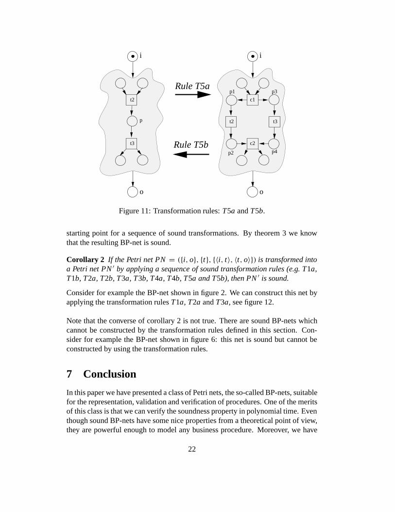
i

o

i

o

t3t2

c2

c1

p2

p1 p3

p4

t2

t3

p

Rule T5a

Rule T5b

Figure 11: Transformation rules: T5a and T5b.

starting point for a sequence of sound transformations. By theorem 3 we knowthat the resulting BP-net is sound.

Corollary 2 If the Petri net PN = ({i, o}, {t}, {〈i, t〉, 〈t, o〉}) is transformed intoa Petri net PN ′ by applying a sequence of sound transformation rules (e.g. T1a,T1b, T2a, T2b, T3a, T3b, T4a, T4b, T5a and T5b), then PN ′ is sound.

Consider for example the BP-net shown in figure 2. We can construct this net byapplying the transformation rules T1a, T2a and T3a, see figure 12.

Note that the converse of corollary 2 is not true. There are sound BP-nets whichcannot be constructed by the transformation rules defined in this section. Con-sider for example the BP-net shown in figure 6: this net is sound but cannot beconstructed by using the transformation rules.

7 Conclusion

In this paper we have presented a class of Petri nets, the so-called BP-nets, suitablefor the representation, validation and verification of procedures. One of the meritsof this class is that we can verify the soundness property in polynomial time. Eventhough sound BP-nets have some nice properties from a theoretical point of view,they are powerful enough to model any business procedure. Moreover, we have

22

fork

i

p1

contact_garage

join

p3

p5

send_letterpay_damage

check_insurance

p2

p4

o

i

o

Rule T1a Rule T2a

i

oo

Rule T3a

i

Figure 12: Construction of the BP-net shown in figure 2.

shown that the plausible transformation rules encountered when reengineering abusiness procedure preserve soundness.

In this paper we focused on the procedure underlying a business process. Tocompletely specify a business process we also have to specify the management ofresources: given a task that needs to be executed for a specific case we have tospecify the resource (person of machine) that is going to process the task (cf. Vander Aalst and Van Hee [5, 4]). A direction for further research is to incorporatethis dimension. We hope to find a necessary and sufficient condition for soundnessgiven a BP-net extended with some mechanism to allocate resources to tasks.

Acknowledgements

The author would like to thank Dr. M. Voorhoeve for his valuable contribution toSection 5.1 and Ir. A.A. Basten for his useful suggestions.

References

[1] W.M.P. van der Aalst. Timed coloured Petri nets and their application to lo-gistics. PhD thesis, Eindhoven University of Technology, Eindhoven, 1992.

[2] W.M.P. van der Aalst. Interval Timed Coloured Petri Nets and their Anal-ysis. In M. Ajmone Marsan, editor, Application and Theory of Petri Nets

23

1993, volume 691 of Lecture Notes in Computer Science, pages 453–472.Springer-Verlag, Berlin, 1993.

[3] W.M.P. van der Aalst. Putting Petri nets to work in industry. Computers inIndustry, 25(1):45–54, 1994.

[4] W.M.P. van der Aalst and K.M. van Hee. Framework for Business ProcessRedesign. In J.R. Callahan, editor, Proceedings of the Fourth Workshop onEnabling Technologies: Infrastructure for Collaborative Enterprises (WET-ICE 95), pages 36–45, Berkeley Springs, April 1995. IEEE Computer Soci-ety Press.

[5] W.M.P. van der Aalst and K.M. van Hee. Business Process Redesign: APetri-net-based approach. Computers in Industry, 29(1-2):15–26, 1996.

[6] E. Best. Structure Theory of Petri Nets: the Free Choice Hiatus. InW. Brauer, W. Reisig, and G. Rozenberg, editors, Advances in Petri Nets1986 Part I: Petri Nets, central models and their properties, volume 254 ofLecture Notes in Computer Science, pages 168–206. Springer-Verlag, Berlin,1987.

[7] E. Best, J. Desel, and J. Esparza. Traps characterize home states in free-choice systems. Theoretical Computer Science, 101:161–176, 1992.

[8] J. Campos, G. Chiola, and M. Silva. Properties and performance boundsfor closed free choice synchronized monoclass queueing networks. IEEETransactions on Automatic Control, 36(12):1368–1381, 1991.

[9] A. Cheng, J. Esparza, and J. Palsberg. Complexity results for 1-safe nets. InR.K. Shyamasundar, editor, Foundations of software technology and theoret-ical computer science, volume 761 of Lecture Notes in Computer Science,pages 326–337. Springer-Verlag, Berlin, 1993.

[10] Bakkenist Management Consultants. ExSpect 4.2 User Manual, 1994.

[11] J. Desel. A proof of the Rank theorem for extended free-choice nets. InK. Jensen, editor, Application and Theory of Petri Nets 1992, volume 616 ofLecture Notes in Computer Science, pages 134–153. Springer-Verlag, Berlin,1992.

[12] J. Desel and J. Esparza. Free Choice Petri Nets, volume 40 of CambridgeTracts in Theoretical Computer Science. Cambridge University Press, Cam-bridge, UK, 1995.

24

[13] J. Esparza. Synthesis rules for Petri nets, and how they can lead to newresults. In J.C.M. Baeten and J.W. Klop, editors, Proceedings of CONCUR1990, volume 458 of Lecture Notes in Computer Science, pages 182–198.Springer-Verlag, Berlin, 1990.

[14] M.H.T. Hack. Analysis production schemata by Petri nets. Master’s thesis,Massachusetts Institute of Technology, Cambridge, Mass., 1972.

[15] K.M. van Hee. Information System Engineering: a Formal Approach. Cam-bridge University Press, 1994.

[16] K. Jensen. Coloured Petri Nets. Basic Concepts, Analysis Methods and Prac-tical Use. EATCS monographs on Theoretical Computer Science. Springer-Verlag, Berlin, 1992.

[17] T. Murata. Petri Nets: Properties, Analysis and Applications. Proceedingsof the IEEE, 77(4):541–580, April 1989.

[18] J.L. Peterson. Petri net theory and the modeling of systems. Prentice-Hall,Englewood Cliffs, 1981.

[19] C.A. Petri. Kommunikation mit Automaten. PhD thesis, Institut fur instru-mentelle Mathematik, Bonn, 1962.

25