A Characterizing Pacific halibut movement and … Pacific halibut movement and habitat in a Marine...
22
MARINE ECOLOGY PROGRESS SERIES Mar Ecol Prog Ser Vol. 517: 229–250, 2014 doi: 10.3354/meps11043 Published December 15 INTRODUCTION Knowledge of fish movement patterns at multiple spatial and temporal scales can benefit the manage- ment of mobile fish species. For example, even highly migratory species that move thousands of kilometers are capable of philopatry at very small spatial scales (Jorgensen et al. 2010). Thus, understanding small scale movement patterns and habitat associations can be an important part of achieving a holistic understanding of stock dynamics and assessing the potential effectiveness of spatial management tech- niques such as marine protected areas (MPAs) for migratory fish species. The Pacific halibut Hippoglossus stenolepis (here- after referred to as ‘halibut’) is an economically, eco- logically, and culturally important flatfish species in the North Pacific Ocean. Based on observations of © Inter-Research 2014 · www.int-res.com *Corresponding author: [email protected] Characterizing Pacific halibut movement and habitat in a Marine Protected Area using net squared displacement analysis methods Julie K. Nielsen 1, *, Philip N. Hooge 2,4 , S. James Taggart 2,5 , Andrew C. Seitz 3 1 School of Fisheries and Ocean Sciences, University of Alaska Fairbanks, 17101 Pt. Lena Loop Rd., Juneau, Alaska 99801, USA 2 US Geological Survey Alaska Science Center, 3100 National Park Road, Juneau, Alaska 99801, USA 3 School of fisheries and Ocean Sciences, University of Alaska Fairbanks, PO Box 757220, University of Alaska Fairbanks, Fairbanks, Alaska 99775, USA 4 Present address: Glacier Bay National Park and Preserve, PO Box 140, Gustavus, Alaska 99826, USA 5 Present address: 1350 Yulupa Ave. Apt. B, Santa Rosa, California 95405, USA ABSTRACT: We characterized small-scale movement patterns and habitat of acoustic-tagged adult (68 to 220 cm total length) female Pacific halibut during summer and fall in Glacier Bay National Park, Alaska, a marine protected area (MPA). We used net squared displacement ana- lysis methods to identify 2 movement states, characterize individual dispersal patterns, and relate habitat variables to movement scales. Movement states identified for 32 of 43 halibut consisted of (1) a non-dispersive ‘residential’ movement state (n = 27 fish), where movement was restricted to an average movement radius of 401.3 m (95% CI 312.2−515.9 m) over a median observation period of 58 d, and (2) a ‘dispersive’ movement state (n = 15 fish), where movements of up to 18 km occurred over a median observation period of 27 d. Some fish (n = 10) exhibited both movement states. Individual fish demonstrated primarily non-random dispersal patterns including home range (n = 17), site fidelity (return to previously occupied locations following forays, n = 6), and shifted home ranges (n = 5). However, we also observed a random dispersal pattern (n = 4) with an estimated mean ± SE diffusion rate of 0.9 ± 0.05 km 2 d −1 . Home range size increased with depth but not fish size. Home range locations were associated with heterogeneous habitat, intermediate tidal velocities, and depths <100 m. Observations of non-dispersive movement patterns, relatively small home ranges, and site fidelity for adult females suggest that MPAs such as Glacier Bay may have utility for conservation of Pacific halibut broodstock. KEY WORDS: Movement ecology · Home range · Site fidelity · Net Squared Displacement · Dispersal · Marine Protected Area · Flatfish · Pacific halibut Resale or republication not permitted without written consent of the publisher FREE REE ACCESS CCESS
Transcript of A Characterizing Pacific halibut movement and … Pacific halibut movement and habitat in a Marine...
MARINE ECOLOGY PROGRESS SERIESMar Ecol Prog Ser
Vol. 517: 229–250, 2014doi: 10.3354/meps11043
Published December 15
INTRODUCTION
Knowledge of fish movement patterns at multiplespatial and temporal scales can benefit the manage-ment of mobile fish species. For example, even highlymigratory species that move thousands of kilometersare capable of philopatry at very small spatial scales(Jorgensen et al. 2010). Thus, understanding smallscale movement patterns and habitat associations
can be an important part of achieving a holisticunderstanding of stock dynamics and assessing thepotential effectiveness of spatial management tech-niques such as marine protected areas (MPAs) formigratory fish species.
The Pacific halibut Hippoglossus stenolepis (here-after referred to as ‘halibut’) is an economically, eco-logically, and culturally important flatfish species inthe North Pacific Ocean. Based on observations of
© Inter-Research 2014 · www.int-res.com*Corresponding author: [email protected]
Characterizing Pacific halibut movement and habitat in a Marine Protected Area using net
squared displacement analysis methods
Julie K. Nielsen1,*, Philip N. Hooge2,4, S. James Taggart2,5, Andrew C. Seitz3
1School of Fisheries and Ocean Sciences, University of Alaska Fairbanks, 17101 Pt. Lena Loop Rd., Juneau, Alaska 99801, USA2US Geological Survey Alaska Science Center, 3100 National Park Road, Juneau, Alaska 99801, USA
3School of fisheries and Ocean Sciences, University of Alaska Fairbanks, PO Box 757220, University of Alaska Fairbanks, Fairbanks, Alaska 99775, USA
4Present address: Glacier Bay National Park and Preserve, PO Box 140, Gustavus, Alaska 99826, USA5Present address: 1350 Yulupa Ave. Apt. B, Santa Rosa, California 95405, USA
ABSTRACT: We characterized small-scale movement patterns and habitat of acoustic-taggedadult (68 to 220 cm total length) female Pacific halibut during summer and fall in Glacier BayNational Park, Alaska, a marine protected area (MPA). We used net squared displacement ana -lysis methods to identify 2 movement states, characterize individual dispersal patterns, and relatehabitat variables to movement scales. Movement states identified for 32 of 43 halibut consisted of(1) a non-dispersive ‘residential’ movement state (n = 27 fish), where movement was restricted toan average movement radius of 401.3 m (95% CI 312.2−515.9 m) over a median observationperiod of 58 d, and (2) a ‘dispersive’ movement state (n = 15 fish), where movements of up to 18 kmoccurred over a median observation period of 27 d. Some fish (n = 10) exhibited both movementstates. Individual fish demonstrated primarily non-random dispersal patterns including homerange (n = 17), site fidelity (return to previously occupied locations following forays, n = 6), andshifted home ranges (n = 5). However, we also observed a random dispersal pattern (n = 4) with anestimated mean ± SE diffusion rate of 0.9 ± 0.05 km2 d−1. Home range size increased with depthbut not fish size. Home range locations were associated with heterogeneous habitat, intermediatetidal velocities, and depths <100 m. Observations of non-dispersive movement patterns, relativelysmall home ranges, and site fidelity for adult females suggest that MPAs such as Glacier Bay mayhave utility for conservation of Pacific halibut broodstock.
KEY WORDS: Movement ecology · Home range · Site fidelity · Net Squared Displacement · Dispersal · Marine Protected Area · Flatfish · Pacific halibut
Resale or republication not permitted without written consent of the publisher
FREEREE ACCESSCCESS
Mar Ecol Prog Ser 517: 229–250, 2014
large-scale seasonal and ontogenetic movementsduring larval, juvenile, and adult life history stages(Valero & Webster 2012), halibut in North Americaare managed on a large scale (Clark & Hare 2006)where a single stock assessment is conducted for a re-gion that ranges from California to the Bering Sea be-fore the allowable harvest is apportioned into smallermanagement units (Webster & Stewart 2014). Someproportion of adult halibut conduct seasonal spawn-ing migrations from summer foraging locations innear-shore areas to winter off-shore spawning areasin deeper waters on the continental slope of the Pa-cific Ocean (Loher & Seitz 2006, Loher 2011, Seitz etal. 2011). Recent pop-up satellite archival taggingand conventional tagging research has de monstratedthat a large proportion of adult halibut exhibit inter-annual site fidelity and homing to summer foraginglocations (Loher 2008). These obser vations suggestthat knowledge of movement patterns at smallerscales will be important for understanding the spatialsub-structure of the halibut stock, potential local ef-fects of intense fishing, and the utility or effectivenessof MPAs as a management tool for halibut.
In addition to coast-wide, large-scale managementthrough area-specific harvest rates, halibut are alsoregulated at smaller spatial scales through catchsharing plans as well as the existence of MPAs. Forexample, halibut harvest is restricted in the interiorwaters of Glacier Bay National Park in southeasternAlaska, where commercial fishing for halibut is beingphased out (36 CFR 13.1130-1146) over several de -cades and sport fishing is limited by daily vessel quotas (36 CFR 13.1150-1160) during the summermonths. Glacier Bay National Park was added to theNational System of Marine Protected Areas in 2009.As a large, high-latitude MPA, Glacier Bay mayeventually protect halibut that reside within itsboundaries from commercial harvest. However, ob -taining information on the scale and patterns of hal-ibut movement and habitat associations is critical forunderstanding Glacier Bay’s potential effectivenessat retention of adults (Kramer & Chapman 1999) andspecific benefits that may result from protection.
Here, we present information on the spatial andtemporal scales of movement by adult halibut in Gla-cier Bay National Park during summer and fall thatmay be valuable for assessing the potential effective-ness of Glacier Bay National Park as an MPA. We usenet squared displacement (NSD) analysis techniquesto (1) identify and characterize 2 distinct movementstates, ‘residential’ and ‘dispersive’, (2) classify andquantitatively describe dispersal patterns for individ-ual tagged halibut, and (3) describe habitat associa-
tions and relationships between habitat variables(depth, average tidal speed, habitat complexity, andsubstrate type) and scale of movement for the resi-dential movement state. We interpret these results interms of spatially explicit fisheries managementapplications such as MPA design and effectiveness.We conclude by addressing the potential contribu-tion of NSD analysis methods for characterizing themovement patterns and dispersal scales of fishes andfacilitating MPA design.
MATERIALS AND METHODS
Study area
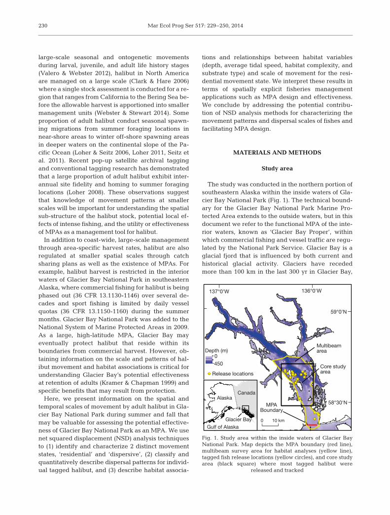
The study was conducted in the northern portion ofsoutheastern Alaska within the inside waters of Gla-cier Bay National Park (Fig. 1). The technical bound-ary for the Glacier Bay National Park Marine Pro-tected Area extends to the outside waters, but in thisdocument we refer to the functional MPA of the inte-rior waters, known as ‘Glacier Bay Proper’, withinwhich commercial fishing and vessel traffic are regu-lated by the National Park Service. Glacier Bay is aglacial fjord that is influenced by both current andhistorical glacial activity. Glaciers have recededmore than 100 km in the last 300 yr in Glacier Bay,
230
136°0'W137°0'W
59°0'N
58°30'N
0 10 km
CanadaAlaska
Gulf of Alaska
Glacier Bay
Depth (m)0450
Multibeamarea
MPABoundary
Release locationsCore studyarea
Fig. 1. Study area within the inside waters of Glacier BayNational Park. Map depicts the MPA boundary (red line),multibeam survey area for habitat analyses (yellow line),tagged fish release locations (yellow circles), and core studyarea (black square) where most tagged halibut were
released and tracked
Nielsen et al.: Movement of Pacific halibut in a Marine Protected Area
leaving behind a Y-shaped body of water with deep(200 to 450 m) marine basins interspersed with shal-low moraines and tidewater glaciers at the heads ofthe fjords. Substantial glacial freshwater runoff in -fluences the oceanography with high sedimentationand areas of cold water upwelling. Strong tidal cur-rents mix the water column completely in the shallowlower portion of the bay, but deeper upper reachesare largely stratified. Primary productivity levels arehighest in a transition zone in the central portion ofthe bay that is characterized by intermediate stratifi-cation. Salinity, temperature, and light penetrationdecrease towards the heads of the fjords (Etheringtonet al. 2007b).
Fish tagging and tracking
A total of 43 halibut were captured on longlines,tagged and released in Glacier Bay during the sum-mers of 1991 to 1993 (Table 1, Fig. 1). Longlines wereset at 4 general release locations within the study areausing snap-on gangions designed for the commercialhalibut fishery and were ‘soaked’ for 6 h. Capture lo-cations were determined when each fish was broughton board the capture vessel using a PLGR GPS thatremoved selective availability errors. We generallyselected larger fish (>100 cm total length, TL) for tag-ging because we were primarily interested in fish thatwere vulnerable to the commercial fishery (≥82 cm)and we wanted to minimize possible effects of large,long-life acoustic tags on behavior.
Acoustic transmitters (Sonotronics) that transmitteda unique identifying sonic pulse were attached to hal-ibut externally during 1991 and 1992 (n = 26) and in-ternally during 1992 and 1993 (n = 17). Externally at-tached acoustic tags were secured to fish by inserting2 Teflon-coated stainless steel wires through the dor-sal musculature immediately ventral to the dorsal fin,with a backing plate of neoprene rubber and fiber-glass. A sterilized needle was used to thread the wire.For the internal attachment, tags were surgically im-planted in the coelomic cavity using sterile methods.Tags were inserted into the coelomic cavity through a5 cm incision on the eyed-side, parallel and 2 to 3 cmdorsal to the long axis of the fish. The incision wasclosed with 7 to 8 external sutures (2-0 Braunamidnon-absorbable). During the 5 to 15 minute surgery,the gills of the fish were irrigated with ambient sea-water which was well-mixed and high-saline in thestudy area. When possible, information on the sex ofthe tagged fish was obtained through cannulation orobservation during surgical implantation. Tagged
fish were released within 500 m of the location wherethey were brought on board.
Acoustic tag transmission frequency and size var-ied during the study. Acoustic tags attached duringthe first year (n = 9) transmitted at a frequency of80 kHz, whereas 35 kHz acoustic tags (n = 34) wereused in the 2 subsequent years due to their increaseddetectability in Glacier Bay’s waters. We used 2 sizesof acoustic tags in the study. The smaller tags (n = 17)were 95 mm long × 18 mm diameter, weighed 16 g inwater, and had an observed lifetime of 1.3 to 2 yr. Thelarger tags (n = 26) were 95 mm long × 34 mm dia -meter, weighed 34 g in water, and had an observedlifetime of 2.5 to 3.4 yr. Details of tag attributes forindividual tagged fish are provided in Table S1 inSupplement 1 at www.int-res.com/articles/suppl/m517p229_supp.pdf.
Tagged halibut were tracked from a vessel using abow-mounted dual hydrophone assembly lowered2 m beneath the surface of the water and capable ofrotating 360°. One hydrophone faced forward and−10° from horizontal and the other hydrophonepointed downward. These directional hydrophones(Sonotronics DH-2) had a beam width of ±6° and asensitivity of 84 dBV and were connected to manualreceivers (Sonotronics USR-4D). With this configura-tion, in situ range tests indicated that tags could bedetected at distances of up to 2 km. When a tag wasdetected, the vessel operator maneuvered the vesselin a circular pattern in the vicinity of the tag until sig-nal strength was uniform at all points on the circleand the signal received on the downward-facinghydrophone in the middle of the circle was highlyamplified. A GPS was used to obtain the location ofthe vessel at this position, which served as the esti-mated position of the tagged fish. Positions of taggedfish were obtained daily to weekly during trackingperiods that lasted 3 to 6 mo, mostly in the summerand fall, of each year. Searches for tagged fish wereconducted in an outward spiral starting from eachindividual’s last known position. Consequently, if atagged halibut moved more than a few kilometersaway, it was not necessarily found during the subse-quent search. An example of the spatial distributionof tracking effort (number of days tracked per sea-son) in the study area during 1991 is shown in Fig. S2in Supplement 1.
The precision of position estimates for tagged fishwas likely to decrease with increasing water depth.We estimated the precision of each observationbased on a linear regression of error radii vs. depthfor (1) known positions of tags recovered by SCUBAdivers (n = 3) and (2) root mean squared distances
231
Mar Ecol Prog Ser 517: 229–250, 2014232
1991
1992
1993
Tag
ged
19
92
Tra
ckin
g
year
Jun
e 1
July
1A
ug
1S
ept
1O
ct 1
Nov
1D
ec 1
Jan
1
# R
elea
se/
Un
kn
own
| R
esid
enti
al|
Dis
per
sive
17/
24/9
113
613
334
6369
FS
HR
27/
30/9
191
2172
1475
HR
38/
20/9
113
614
9215
0H
R4
8/20
/91
115
––
N5
8/20
/91
140
9796
9614
SH
R6
8/20
/91
7817
7898
4H
R7
8/20
/91
9020
3131
9H
R8
9/9/
9196
1417
714
177
R9
9/9/
9111
796
1980
23S
HR
106/
3/92
157
3691
2027
FS
HR
116/
17/9
212
816
658
1147
2U
126/
19/9
294
––
N13
6/19
/92
6845
5845
58U
146/
19/9
276
.576
276
2U
156/
23/9
215
387
437
8H
R16
7/1/
9212
992
9141
8S
F17
7/1/
9210
423
9023
90R
187/
8/92
146
2269
1497
HR
197/
8/92
127
2163
2163
U20
7/8/
9213
2.5
1339
313
393
SH
R21
7/8/
9212
118
4821
3H
R22
7/8/
9212
481
8419
09S
F23
7/8/
9214
2.5
237
237
U24
7/8/
9213
416
478
1647
8R
257/
8/92
125
1261
639
93S
F26
7/8/
9212
912
494
3839
SF
277/
31/9
220
1.3
2014
1296
HR
2811
/17/
9213
0.6
9188
207
SF
2911
/17/
9214
910
872
496
SF
3011
/17/
9213
2.5
1652
497
U31
11/1
7/92
168
614
73H
R32
6/2/
9322
031
9019
49H
R33
6/18
/93
154
1795
415
963
R34
6/18
/93
162
––
N35
6/18
/93
151.
2–
–N
366/
19/9
314
011
7056
7H
R37
6/19
/93
182.
835
2626
14H
R38
6/19
/93
155
859
843
HR
396/
19/9
315
1.6
––
N40
6/20
/93
152.
822
6950
7H
R41
6/20
/93
149.
811
0972
6H
R42
6/20
/93
164.
412
9635
9H
R43
8/11
/93
77.6
807
619
HR
100
150
200 D
ay o
f th
e ye
ar250
350
300
Fis
h
IDR
elea
se
Dat
eL
eng
th
(cm
)M
ax
dis
p. (
m)
Net
d
isp
. (m
)M
odel
co
de
# //|||
|||
|||
||||||
||||
|||
||||
||
||||
|||
# ///
|||
||
|||||
|||||
|||||
|||
||||
|||
|||
||||
|||
|||
||
|# //
/|||
||||
|||||
||||
||||
|||
|||
||||
|||
|||
||# # //
/||||
||||
||||
|||
|||
|||
||||
|||
|||
||
||
|||
||
# //|
|||||
|||
|||
||||
||||
||
|||
|#
//|
|||||
|||
|||
||||
||||
||||
|||
|||
||
#|
|# /
/|
|||
||
|||
||||
|||
||
|||
||
|
#|
||||
||||
|||
||
|||#|
||
||||
# # #|
||||
||
||||
#|
|||
|||
|||
||
#|
||||
||||
||
||||
# #||
||||
|||
||
|||#
/||
||||
|||
||
|||#
/||
||||
|||
||
|||
# #/
# /#|
||#
|||
||
|||
|||
||
|||
||
||
|
#||
|||
|||||
|||||
||||
|||
|||
||
||
|# /|
|||
|||||
||||
||||
||||
||||||
||||
|||
||||
|||
#||| # /
/||
||
|||
|||||
|||
||
||||
||||
||||
||||
|||
# / # /||
||
# //
||
|||
|||||
|||
||||
||#
|||
|||||
|||||
|||
||
# / #|||
|||||
#||
||
|||||
||||
|||||
|#|
|||
|||
||||||
||
||||
#/|
|||
||||||
|||
||||
|||
||
|||
|
#|
|||
|||
||||
|||
||
|||#|
||
|||
|||
||
||
||||
||||
||
||||
# //
# //
|||
||||
||
||
||
||||
||||
||
||||
# /|
|||
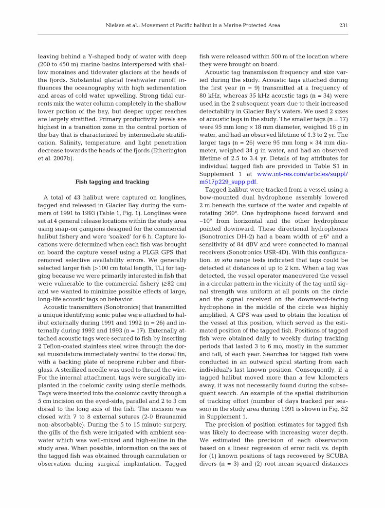
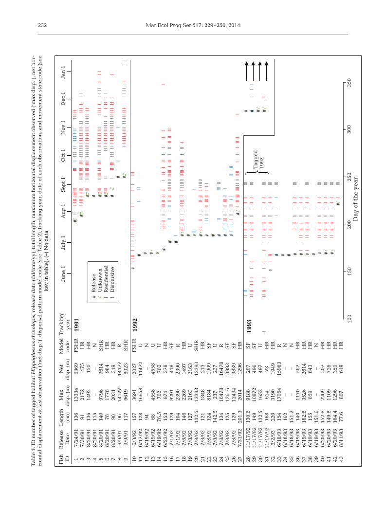
Tab
le 1
. ID
nu
mb
er o
f tag
ged
hal
ibu
t Hip
pog
loss
us
sten
olep
is, r
elea
se d
ate
(dd
/mm
/yy)
, tot
al le
ng
th, m
axim
um
hor
izon
tal d
isp
lace
men
t ob
serv
ed (‘
max
dis
p.’)
, net
hor
-iz
onta
l dis
pla
cem
ent
at la
st o
bse
rvat
ion
(‘n
et d
isp
.’), d
isp
ersa
l pat
tern
mod
el c
ode
(see
Tab
le 2
), t
rack
ing
yea
r, d
ate
of e
ach
ob
serv
atio
n, a
nd
mov
emen
t st
ate
cod
e (s
ee
key
in t
able
). (
–) N
o d
ata
Nielsen et al.: Movement of Pacific halibut in a Marine Protected Area
between repeated observations of motionless tags (n= 6). The depth of each observation was multi plied bythe resulting slope coefficient, 0.65 (r2 = 0.83, p =0.0005), to obtain error buffers for each observationthat ranged from approx. ±10 m at depths of 10 m toapprox. ±100 m at depths of 150 m.
Data analysis
Due to the large study area and the opportunisticnature of the fish resightings, the dataset was charac-terized by irregular sampling intervals, un equal sam-ple sizes among fish, and small numbers of observa-tions for some fish. Because most movement analysismethods require regular and frequent observationsof tagged fish, we employed an alternative analysisframework that is robust to missing data and smallsample sizes. This analysis framework, based on thenet squared displacement (NSD) statistic, is based onthe identification of patterns of dispersal over timethat correspond to different behaviors such as forag-ing or migration (Börger & Fryxell 2012). NSD, alsocommonly referred to as R2
n, is the square of the dis-tance between the origin of a given trajectory andeach subsequent position.
NSDt = �xt – x0 �2 (1)
where xt is the coordinate vector at time t (i.e. the
latitude and longitude of a fish on day t), and x0 is thecoordinate vector for the origin of the trajectory (i.e.a fish’s release location). For random movement, e.g.Brownian motion, the NSD statistic increases linearlywith time (Kareiva & Shigesada 1983) and the slope isproportional to the rate of diffusion (Börger & Fry xell2012). For non-dispersive movement, such as homerange behavior, the NSD statistic reaches a constantvalue over time that represents the spatial scale of thearea in which the fish moves (Turchin 1998, Moorcroft& Lewis 2006). For directed movement toward a spe-cific location, such as during migration or moving be-tween foraging locations, the relationship betweenNSD and time is exponential (Nouvellet et al. 2009).
Movement states
We defined 2 different movement states using theNSD statistic. The first movement state, ‘residential,’reflects non-dispersive movement and was definedwhen the slope of NSD vs. time = 0 (p > 0.05 for theslope coefficient in a linear regression) for a mini-mum sample size of 4 consecutive observations(Fig. 2). For this movement state, the intercept ofNSD vs. time provides information about the spatialscale at which NSD values do not increase or de -crease over time, thus providing an estimate of homerange size that is robust to small sample sizes and
233
0
6 x 10⁷
0
6 x 10⁷
0 2 km
Fish ID
3
5
Release location
3
5
Depth (m)
-250
-200
-150
-100
-50
Day of the year
NS
D (m
2 )
Home rangedispersal pattern
R = residentialD = dispersive
A B
Home range Foray
Shifted home range
C Shifted home rangedispersal pattern
RD
R
RD
240 260 280 300 320 340
240 260 280 300 320 340
R
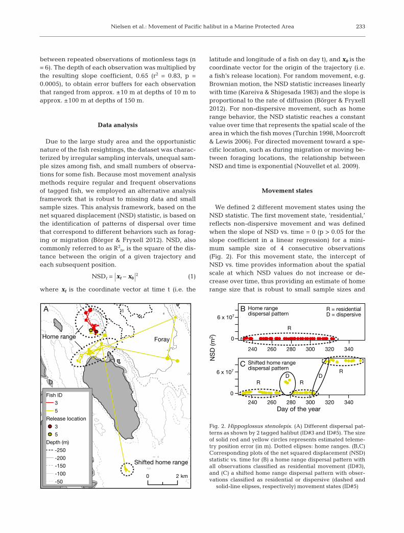
Fig. 2. Hippoglossus stenolepis. (A) Different dispersal pat-terns as shown by 2 tagged halibut (ID#3 and ID#5). The sizeof solid red and yellow circles represents estimated teleme-try position error (in m). Dotted elipses: home ranges. (B,C)Corresponding plots of the net squared displacement (NSD)statistic vs. time for (B) a home range dispersal pattern withall observations classified as residential movement (ID#3),and (C) a shifted home range dispersal pattern with obser-vations classified as residential or dispersive (dashed and
solid-line elipses, res pectively) movement states (ID#5)
Mar Ecol Prog Ser 517: 229–250, 2014
infrequent observations (Moorcroft & Lewis 2006).Consecutive observations classified as residential aresubsequently referred to as ‘home ranges’. We esti-mated typical home range size for the residentialmovement state using an intercept-only linearmixed-effects model:
log(NSD)ij = α + ai + εij (2)ai ~ N(0,σ2
a), εij ~ N(0, σ2)
where α is the fixed-effects estimate of mean homerange size for the population of i home ranges, ai is arandom variable that represents the variation of indi-vidual home range estimates around the fixed-effectsmean, and within-group error εij is assumed to beindependent and normally distributed with a mean ofzero. The model was fit using restricted maximumlikelihood. NSD values were log-transformed to ac -count for heteroscedasticity prior to modeling. Weapplied the bias-correction for a log-normal distribu-tion to back-transform the estimated mean to theoriginal scale:
Home range size (NSD) = exp(α + s2/2) (3)
where α is the mean home range size for the popula-tion as described above and s2 is the estimated vari-ance for α. To provide a more intuitive linear descrip-tion of movement scale, the square root of interceptcoefficients were reported as a ‘home range radius.’To minimize potential bias of capture and tagging onthe scale of home range movement patterns (e.g.temporary tagging effects, uncertainty in longlineposition during capture vs. release location, or travelfrom release position back to the home range), obser-vations within 3 d of tagging were not used for homerange analyses.
The second movement state, ‘dispersive,’ was clas-sified as all observations where the slope of NSD vs.time ≠ 0 (Fig. 2C). This movement state generallycontained observations from both random and direc -ted movement types. Because fish with more mobilemovement patterns were more difficult to relocate,observations were not collected frequently enough todetermine whether individual observation sequenceswere random (linear relationship for NSD vs. time) ordirected (exponential relationship for NSD vs. time).Therefore, we did not summarize this movementstate using a mixed-effects model, as we did for theresidential movement state, because it likely con-tained a mix of both movement types.
Although we were not able to explicitly classify ob -servations as either random or directed, insight intothe randomness of the dispersive movement state
was obtained by comparing our observations of aver-age NSD vs. time to expected random values usingcorrelated random walks (CRWs). CRWs are move-ment paths comprised of a discrete series of move-ment steps where the expected distance and theexpected angle between subsequent steps deter-mines overall movement path characteristics such asdiffusion rates (larger for larger step lengths) anddirected vs. random movement (more directed forsmaller variation in turning angles, more random forlarger variation in turning angles). CRWs are usuallysimulated based on empirical distributions of bothstep lengths and turning angles obtained from fre-quent and regular observations of a fish’s locationover time (Kareiva & Shigesada 1983, Turchin 1998).However, because our dataset was highly irregular,we simulated random movement from a step lengthdistribution comprised of all records that were 1 dapart, but used a theoretical distribution of turningangles (wrapped Cauchy with an autocorrelationcoefficient of 0.5) that is typically observed duringfish foraging activities (Morales et al. 2004, Bar-tumeus et al. 2005). This approach allowed us toincorporate empirical information on spatial scales ofour tagged fish (daily step lengths) under a specifichypothesis of random movement during for aging. Wefit exponential curves (Moorcroft & Lewis 2006) toboth the residential and dispersive step length distri-butions and sampled randomly from these distribu-tions to create 1000 CRWs for a duration of 90 d foreach movement state. To account for the effects ofmovement that occurs within the confined waters ofthe study area, simulations were conducted on a 20 mbathymetry grid of Glacier Bay (Geiselman et al.1997) and were initiated at the first location of eachobserved residential or dispersive movement se -quence. If a simulated position for the CRW fell onland, that position was discarded and a new coordi-nate was chosen. To assess randomness, the meanNSD from observed data was compared to the meanand 95% CI from the CRWs at each time step. NSDvalues for random movement should fall within the95% CI for the CRW simulations, whereas values fordirected and non-dispersive movement will begreater than the upper bound and less than the lowerbound, respectively, of the 95% CI for CRW values(Austin et al. 2004).
Individual dispersal patterns
In addition to characterization of movement states,knowledge of the way in which NSD changes over
234
Nielsen et al.: Movement of Pacific halibut in a Marine Protected Area
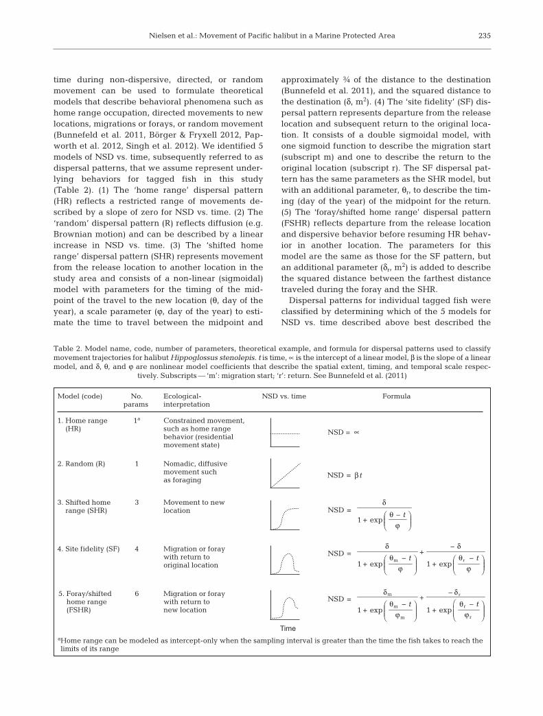
time during non-dispersive, directed, or randommovement can be used to formulate theoreticalmodels that describe behavioral phenomena such ashome range occupation, directed movements to newlocations, migrations or forays, or random movement(Bunnefeld et al. 2011, Börger & Fryxell 2012, Pap-worth et al. 2012, Singh et al. 2012). We identified 5models of NSD vs. time, subsequently referred to asdispersal patterns, that we assume represent under-lying behaviors for tagged fish in this study(Table 2). (1) The ‘home range’ dispersal pattern(HR) reflects a restricted range of movements de -scribed by a slope of zero for NSD vs. time. (2) The‘random’ dispersal pattern (R) reflects diffusion (e.g.Brownian motion) and can be described by a linearincrease in NSD vs. time. (3) The ‘shifted homerange’ dispersal pattern (SHR) represents movementfrom the release location to another location in thestudy area and consists of a non-linear (sigmoidal)model with parameters for the timing of the mid-point of the travel to the new location (θ, day of theyear), a scale parameter (ϕ, day of the year) to esti-mate the time to travel between the midpoint and
approximately ¾ of the distance to the destination(Bunnefeld et al. 2011), and the squared distance tothe destination (δ, m2). (4) The ‘site fidelity’ (SF) dis-persal pattern represents departure from the releaselocation and subsequent return to the original loca-tion. It consists of a double sigmoidal model, withone sigmoid function to describe the migration start(subscript m) and one to describe the return to theoriginal location (subscript r). The SF dispersal pat-tern has the same parameters as the SHR model, butwith an additional parameter, θr, to describe the tim-ing (day of the year) of the midpoint for the return.(5) The ‘foray/shifted home range’ dispersal pattern(FSHR) reflects departure from the release locationand dispersive behavior before re suming HR behav-ior in another location. The parameters for thismodel are the same as those for the SF pattern, butan additional parameter (δr, m2) is added to describethe squared distance between the farthest distancetraveled during the foray and the SHR.
Dispersal patterns for individual tagged fish wereclassified by determining which of the 5 models forNSD vs. time described above best described the
235
NSD = ∝
Model (code) NSD vs. time Formula
1. Home range (HR)
2. Random (R)
NSD = βt
3. Shifted home range (SHR) NSD =
NSD =
NSD =
4. Site fidelity (SF)
5. Foray/shifted home range (FSHR)
Ecological-interpretation
Constrained movement,such as home range behavior (residential movement state)
Nomadic, diffusivemovement such as foraging
Migration or foraywith return to original location
Movement to newlocation
Migration or foraywith return to new location
aHome range can be modeled as intercept-only when the sampling interval is greater than the time the fish takes to reach the limits of its range
⎟⎟⎠⎞
⎜⎜⎝⎛
ϕ−θ
+
δ
texp1
⎟⎟⎠⎞
⎜⎜⎝⎛
ϕ−θ
+
δ−+
⎟⎟⎠⎞
⎜⎜⎝⎛
ϕ−θ
+
δtt rm
exp1exp1
⎟⎟⎠
⎞⎜⎜⎝
⎛ϕ
−θ+
δ−+
⎟⎟⎠
⎞⎜⎜⎝
⎛ϕ
−θ+
δ
r
r
r
m
m
m
ttexp1exp1
Time
No.params
1a
1
3
4
6
Table 2. Model name, code, number of parameters, theoretical example, and formula for dispersal patterns used to classifymovement trajectories for halibut Hippoglossus stenolepis. t is time, ∝ is the intercept of a linear model, β is the slope of a linearmodel, and δ, θ, and ϕ are nonlinear model coefficients that describe the spatial extent, timing, and temporal scale respec-
tively. Subscripts — ‘m’: migration start; ‘r’: return. See Bunnefeld et al. (2011)
Mar Ecol Prog Ser 517: 229–250, 2014
observed values of NSD vs. time based on modelselection techniques. Non-linear models (all modelsbesides HR and random) were fit using a non-linearleast squares algorithm (the nls function in the ‘stat’package for R). The best-fitting model for each indi-vidual trajectory was selected using the AkaikeInformation Criterion adjusted for small samplesizes (AICc) (Burnham & Anderson 1990) and resid-ual analysis. An example of the dispersal patternclassification process for individual fish is providedin Fig. S3 in Supplement 2 at www.int-res. com/articles/suppl/ m517 p229_ supp. pdf. Once individualfish were classified according to dispersal pattern,we calculated the average for: (1) maximum dis-tance from the release location during the observa-tion period, (2) distance from the release location atthe end of the observation period, (3) observationperiod duration, and (4) fish size for each dispersalpattern.
We used mixed-effects models to summarize modelparameters for dispersal patterns to which more than3 fish were assigned. Because fish with the HR dis-persal pattern were included in the mixed-effectsmodel for the residential movement state, mixed-effects models were only used to summarize the ran-dom and SF dispersal patterns. For the random dis-persal pattern, we quantified the rate of dispersalover time using a linear model with no intercept, as,by definition, dispersal must be zero at the origin of atrajectory, using fish ID as a grouping variable.
NSDij = βt + bit + εij (4)bi ~ N(0,σ2
b), εij ~ N(0, σ2)
where β is the fixed-effect variable estimate of themean slope of NSD vs. time for the population of irandom trajectories, bi is a random variable that re -presents the variation of individual slopes around thepopulation mean slope, and within-group error εij is arandom variable that is independent and normallydistributed with a mean of 0. The model was fit usingrestricted maximum likeli hood. Because randommovement results in the process of diffusion, NSD vs.time for random movement is proportional to diffu-sion. Therefore, results are presented in the form ofthe estimated rate of diffusion, in km2 d−1, which iscalculated by dividing the slope of NSD vs. time by 4for movement in 2 dimensions (Börger & Fryxell2012).
For the SF dispersal pattern, we quantified timing,duration, and distance traveled during forays thatoccurred during the summer with a non-linearmixed-effects model:
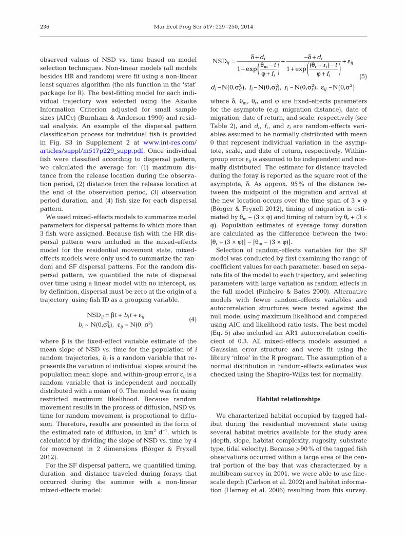
(5)
where δ, θm, θr, and ϕ are fixed-effects parametersfor the asymptote (e.g. migration distance), date ofmigration, date of return, and scale, respectively (seeTable 2), and di , fi , and ri are random-effects vari-ables assumed to be normally distributed with mean0 that represent individual variation in the asymp-tote, scale, and date of return, respectively. Within-group error εij is assumed to be independent and nor-mally distributed. The estimate for distance traveledduring the foray is reported as the square root of theasymptote, δ. As approx. 95% of the distance be -tween the midpoint of the migration and arrival atthe new location occurs over the time span of 3 × ϕ(Börger & Fryxell 2012), timing of migration is esti-mated by θm − (3 × ϕ) and timing of return by θr + (3 ×ϕ). Population estimates of average foray durationare calculated as the difference be tween the two: [θr + (3 × ϕ)] − [θm − (3 × ϕ)].
Selection of random-effects variables for the SFmodel was conducted by first examining the range ofcoefficient values for each parameter, based on sepa-rate fits of the model to each trajectory, and selectingparameters with large variation as random effects inthe full model (Pinheiro & Bates 2000). Alternativemodels with fewer random-effects variables andautocorrelation structures were tested against thenull model using maximum likelihood and comparedusing AIC and likelihood ratio tests. The best model(Eq. 5) also included an AR1 auto correlation coeffi-cient of 0.3. All mixed-effects models assumed aGaussian error structure and were fit using thelibrary ‘nlme’ in the R program. The as sumption of anormal distribution in random-effects estimates waschecked using the Shapiro-Wilks test for normality.
Habitat relationships
We characterized habitat occupied by tagged hal-ibut during the residential movement state using several habitat metrics available for the study area(depth, slope, habitat complexity, rugosity, substratetype, tidal velocity). Because >90% of the tagged fishobservations occurred within a large area of the cen-tral portion of the bay that was characterized by amultibeam survey in 2001, we were able to use fine-scale depth (Carlson et al. 2002) and habitat informa-tion (Harney et al. 2006) resulting from this survey.
NSD1 exp 1 exp
( )
~N(0, ), ~ N(0, ), ~N(0, ), ~N(0, )
m r
2 2 2 2
dt
f
dr tf
d f r
iji
i
i
i
i
ij
i d i f i r ij
( ) ( )= δ +
+ θ −ϕ +
+ −δ +
+ θ + −ϕ +
+ ε
σ σ σ ε σ
236
Nielsen et al.: Movement of Pacific halibut in a Marine Protected Area
However, observations for 2 tagged fish were re -moved from habitat analyses because a majority oftheir observations fell outside of the multibeam studyarea. Continuous rasters for slope, change-in-slope(an indicator of slope interfaces and measure of habi-tat complexity), and rugosity (a measure of surfaceroughness) were derived from 5 m resolution depthdata using ArcGIS 10.0 Spatial Analyst and ArcGIS10.1 Benthic Terrain Modeler (Wright et al. 2012,ESRI 2011). Continuous rasters for soft sediment andmoderate habitat complexity were derived from dis-crete habitat map polygons by calculating Euclideandistance from each grid cell to each type of polygon.Continuous information on time and depth averaged(monthly) tidal velocity was available from a 2-dimensional circulation model (ADCIRC) of GlacierBay (Etherington et al. 2007b, Hill et al. 2009). Weused information from these 7 continuous rasters(depth, slope, change-in-slope, rugosity, distance fromsoft sediment, distance from moderate complexityhabitat, and tidal velocity) to identify habitat associa-tions and quantify the effects of habitat variables onHR size. Study area maps and additional details onhabitat raster characteristics are available in Supple-ment 3 (Fig. S4, Table S3) at www.int-res . com/ articles/suppl/m517p229_supp.pdf.
Habitat associations. To provide a simple descrip-tion of the predominant habitat characteristics ob -served for the residential movement state relative toall available habitat types in the study area, we adap -ted an approach used to detect habitat associationsbased on the spatial distribution of catch during trawlsurveys (Perry & Smith 1994). This method involvescomparing the cumulative distribution function (CDF)of habitat values (e.g. depth) where tagged fish wereobserved to the CDF of available depths in the studyarea. Because halibut are large-bodied fish capableof a high degree of movement, we assumed theycould have moved anywhere in the study area overthe course of the observation period. To obtain CDFsfor available habitat in the study area, a 20 m grid ofthe study area was created in ArcGIS (1.08 × 10⁶
points) and values from each habitat raster wereextracted at each grid point.
To account for telemetry error in the habitat ana -lyses, a buffer with a radius of the estimated errorwas drawn around each tagged fish observation andall grid values within the buffer were averaged. ‘Ob -served’ CDFs were then calculated using the medianvalue of all observations in each HR to avoid pseudo-replication from treating repeated, irregular observa-tions of 1 fish at 1 location as independent events(Rogers & White 2007). Confidence intervals for
observed CDFs were generated by bootstrapping,where the median observation for each HR was sam-pled with replacement 1000 times, and the 0.975 andthe 0.025 quantile values were selected as the upperand lower confidence intervals.
We defined habitat associations by quantitativelycomparing the CDFs for observed and available fishhabitat. Specifically, for each habitat variable, weused the bootstrapped confidence levels for the ob -served CDFs to test for differences between obser -ved and available habitat using the Kolmogorov-Smirnov (K-S) test. The K-S test is frequently used totest for differences between CDFs based on the max-imum vertical difference (D) between the CDFs(Conover 1999). To determine whether positive dif-ferences existed between the observed and availableCDFs (e.g. an association with shallower depths), wefound the greatest positive difference (D+) betweenthe upper CI of the observed CDF and the availableCDF. To determine whether negative differences ex -isted between the observed and available CDFs (e.g.an association with deeper depths), we found thegreatest negative difference (D−) between the lowerCI of the observed CDF and the available CDF. Wedetermined D+, D−, and p-values for each habitatvariable using one-tailed Kolmogorov-Smirnov tests.
Habitat and home range size. We used a general-ized additive model (GAM) to determine whether HRsizes were related to habitat variables or fish totallength. Intercept coefficients from the mixed-effectsmodel for the residential movement state (in log for-mat) were used as the response variable. Explana-tory habitat variables were selected from the 7 con-tinuous habitat rasters used for habitat associationanalyses. In addition to habitat variables, we alsoincluded fish total length and year of study as ex -planatory variables for HR size. The GAM ap proachwas used to allow for potential non-linearities in therelationship between response and ex planatory vari-ables. Prior to analysis, all variables were checked forcovariance with the Pearson correlation coefficient; ifa set of variables were found to be correlated, onlythe variable with the strongest relationship with theresponse variable was used in the model. After as -sessing correlation and linearity of habitat variables,2 full models were tested:
Model 1: y = α + s1 (depth, k = 2) + s2 (fish total length,k = 3) + s3 (distance from moderate complexity, k = 3)+ β1 change-in-slope + β2 tidal velocity + year + ε (6)
Model 2: y = α + s1 (depth, fish total length, k = 3) + s3 (distance from moderate complexity, k = 3) + β1 change-in-slope + β2 tidal velocity + year + ε (7)
237
Mar Ecol Prog Ser 517: 229–250, 2014
where y is the vector of estimated intercepts from themixed-effects model for all residential trajectory seg-ments (n = 29), α and βi are regression coefficients, si
are smooth functions of the predictor variables, krepresents the degree of smoothing in the smoothfunctions, and ε are the residuals, assumed to beindependent and normally distributed. GAM modelswere fit using maximum likelihood methods with aGaussian error structure in the mgcv package in R(Wood 2006). Variables were sequentially removedfrom a full model based on the highest p-value (i.e.larger than 0.05) and the best model was chosenbased on the AICc criterion and residual analysis.
RESULTS
Fish tagging and tracking
A total of 43 fish were tagged between 1991 and1993 (Table 1). Most fish were tagged between Juneand September of each year, but 4 fish were taggedin November 1992 and tracked during the followingsummer, and all were released in good condition.Tagged fish TL (mean ± SD) was 133 ± 32 cm. Almostall (16 of 18) of the fish that we were able to sex werefemale; however, sex could not be determined forthe majority (n = 25) of tagged halibut in this study.Based on fish size and maturity ogives from Interna-tional Pacific Halibut Commission (IPHC) recordsduring this time period, the majority of the halibuttagged in this study were likely to be adult females(T. Loher pers. comm.).
Five fish were never relocated following tagging(Table 1). For the remaining 38 fish, the mean (±SD)number of relocations per fish was 17.4 ± 14.3 andranged from 1 to 49. More than half of the relocationsfor individual fish were obtained within 3 d of theprevious observation, and 90% of the subsequentobservations in each tracking period were within 8 dof the previous observation. Thus, the temporal scaleof tagged fish observations during each trackingperiod can be characterized as daily to weekly. Intotal, 706 acoustic tracking position estimates wereobtained for all tagged fish in all years. Trackingeffort differed among years, with most intense track-ing during 1991 (32.5 observations per fish) anddecreasing during 1992 (13.4 observations per fish)and 1993 (14.8 observations per fish). Tagged fishwere observed over a mean tracking duration of79.5 d (range 1 to 290 d) each year.
The average (±SE) distance that individual taggedfish (n = 38) moved between the release location
and the location of the last observation was 3.5 ±0.8 km. The average (±SE) maximum distance trav-eled during the entire observation was 5.8 ± 0.9 km.The maximum distance from release location re -corded during the study was 17.9 km (Table 1).There were no significant relationships between themaximum distance traveled for each fish and fishsize (linear regression, p = 0.709), tag size: bodyweight ratio (linear regression, p = 0.637), tag size(small vs. large; ANOVA, p = 0.146), or tag attach-ment method (interval vs. external; ANOVA, p =0.797).
Movement states
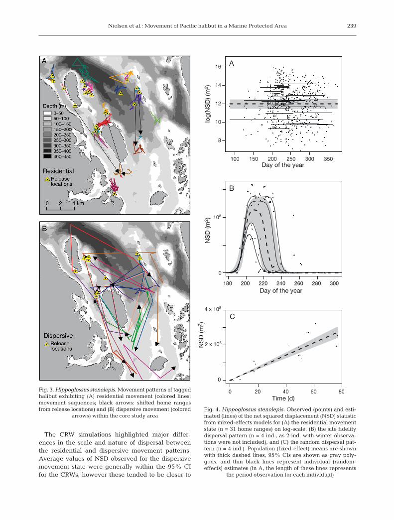
The residential movement state was observed mostfrequently (27 of 43 tagged halibut; Fig. 3A). A totalof 31 residential movement sequences (some fish hadmore than 1 residential sequence) were observedwith a median duration of 58 d. The mixed-effectsmodel population estimate (mean ± SE) for the inter-cept of NSD vs. time was 12.0 ± 0.3 m2, with a stan-dard deviation for random effects of 1.4 on the logscale (Fig. 4A). This corresponds to an estimatedpopulation HR radius of 401.3 m (95% CI = 312.2−515.9 m) and 95% CIs for individual HR radii thatrange from 104.3 to 1493.9 m on the untransformedscale.
The dispersive movement state was observed for15 of 43 tagged halibut (Table 1, Fig. 3B). A total of 18dispersive movement sequences were observed witha median duration of 27 d. This duration was signifi-cantly shorter than that of the residential movementstate (t-test, p < 0.0001). The average maxi mum dis-tance from the release location for fish that exhibitedthe dispersive movement state was 10.9 km.
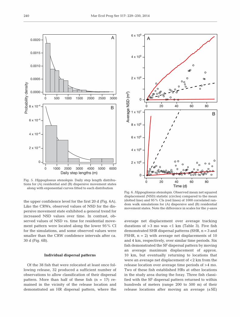
The step length distribution for the residentialmovement state (Fig. 5A) was significantly differentthan the step length distribution for the dispersivemovement (Fig. 5B). Based on a randomization testwith 1000 permutations, the median daily movementstep length for observations from the residentialmovement state (330.4 m, n = 193 observations) wassignificantly less (p < 0.0001) than the median dailymovement step length for observations from the dis-persive movement state (861 m, n = 19 observations).The rate parameter for the exponential curve thatwas fit to each step length distribution for use in theCRW analyses was 0.000213 ± 0.000015 (SE) forobservations from the residential movement stateand 0.0008059 ± 0.000184 for observations from thedispersive movement state.
238
Nielsen et al.: Movement of Pacific halibut in a Marine Protected Area
The CRW simulations highlighted major differ-ences in the scale and nature of dispersal betweenthe residential and dispersive movement patterns.Average values of NSD observed for the dispersivemovement state were generally within the 95% CIfor the CRWs, however these tended to be closer to
239
Fig. 3. Hippoglossus stenolepis. Movement patterns of tag gedhalibut exhibiting (A) residential movement (colored lines:movement sequences; black arrows: shifted home rangesfrom release locations) and (B) dispersive movement (colored
arrows) within the core study area
log(
NS
D) (
m2 )
NS
D (m
2 )N
SD
(m2 )
100 150 200 250 300 350
8
10
12
14
16 A
0
0
0
4 x 10⁸
108
2 x 10⁸
20 40 60 80Time (d)
C
180 200 220 240 260 280 300Day of the year
Day of the year
B
Fig. 4. Hippoglossus stenolepis. Observed (points) and esti-mated (lines) of the net squared displacement (NSD) statisticfrom mixed-effects models for (A) the residential movementstate (n = 31 home ranges) on log-scale, (B) the site fidelitydispersal pattern (n = 4 ind., as 2 ind. with winter observa-tions were not included), and (C) the random dispersal pat-tern (n = 4 ind.). Population (fixed-effect) means are shownwith thick dashed lines, 95% CIs are shown as gray poly-gons, and thin black lines represent individual (random- effects) estimates (in A, the length of these lines represents
the period observation for each individual)
Mar Ecol Prog Ser 517: 229–250, 2014
the upper confidence level for the first 20 d (Fig. 6A).Like the CRWs, observed values of NSD for the dis-persive movement state exhibited a general trend forincreased NSD values over time. In contrast, ob -served values of NSD vs. time for residential move-ment pattern were located along the lower 95% CIfor the simulations, and some observed values weresmaller than the CRW confidence intervals after ca.30 d (Fig. 6B).
Individual dispersal patterns
Of the 38 fish that were relocated at least once fol-lowing release, 32 produced a sufficient number ofobservations to allow classification of their dispersalpattern. More than half of these fish (n = 17) re -mained in the vicinity of the release location anddemonstrated an HR dispersal pattern, where the
average net displacement over average trackingdurations of >3 mo was <1 km (Table 3). Five fishdemonstrated SHR dispersal patterns (SHR, n = 3 andFSHR, n = 2) with average net displacements of 10and 4 km, respectively, over similar time periods. Sixfish demonstrated the SF dispersal pattern by movingan average maximum displacement of approx.10 km, but eventually returning to locations thatwere an average net displacement of <2 km from therelease location over average time periods of >4 mo.Two of these fish established HRs at other locationsin the study area during the foray. Three fish classi-fied with the SF dispersal pattern returned to withinhundreds of meters (range 200 to 500 m) of theirrelease locations after moving an average (±SE)
240
0 500 1000 1500 2000 2500 3000
0.0000
0.0005
0.0010
0.0015
0.0020 A
Daily step lengths (m)
Pro
bab
ility
den
sity
0 1000 2000 3000 4000 5000 6000
0
4 x 10⁻⁴
2 x 10⁻⁴
6 x 10⁻⁴
8 x 10⁻⁴B 0 20 40 60 80
0
2 x 10⁸
4 x 10⁸
6 x 10⁸
A
0 20 40 60 80
0
2 x 10⁶
4 x 10⁶
6 x 10⁶
8 x 10⁶
1 x 10⁷
B
Ave
rage
NS
D (m
2 )
Time (d)
Fig. 5. Hippoglossus stenolepis. Daily step length distribu-tions for (A) residential and (B) dispersive movement states
along with exponential curves fitted to each distributionFig. 6. Hippoglossus stenolepis. Observed mean net squareddisplacement (NSD) statistic (circles) compared to the mean(dotted line) and 95% CIs (red lines) of 1000 correlated ran-dom walk simulations for (A) dispersive and (B) residentialmovement states. Note the difference in scales for the y-axes
Nielsen et al.: Movement of Pacific halibut in a Marine Protected Area
maximum distance of 9.8 km ±0.5 km. One fish classified as SHR(ID#5, Fig. 2) also demonstrated a SFpattern during a temporary foray of6 km and duration of 16 d followed bya return to within 200 m of the loca-tion occupied prior to the foray. Fourfish exhibited the random (R) disper-sal pattern, moving an average maxi-mum and average net displacementof approx. 12 km over observationperiods that averaged <2 mo (approx-imately half of the typical durationsobserved for the fish assigned to otherdispersal patterns). The 6 fish forwhich only a few observations were collected (U) had very short observa-tion durations (average 13.5 d), yetthe average net displacement ofapprox. 3 km for these fish wasgreater than that observed for the HRdispersal pattern. There was no significant difference among the totallengths of fish in each of the 5 disper-sal patterns, un classified movements,or the fish that were never obser vedafter tagging (Kruskal-Wallis test, p =0.3679, df = 6).
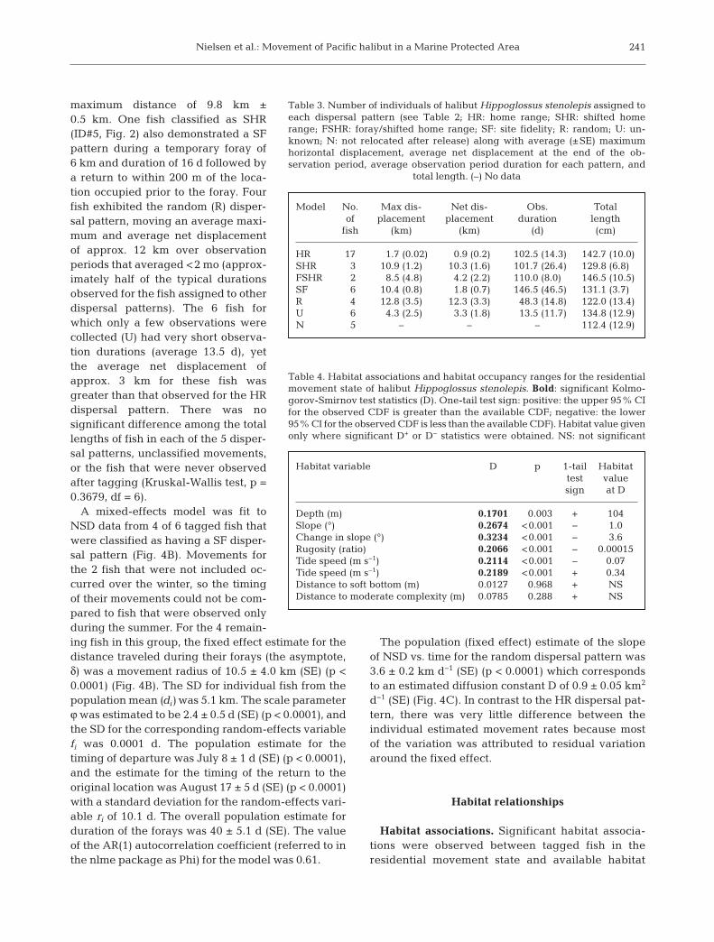
A mixed-effects model was fit toNSD data from 4 of 6 tagged fish thatwere classified as having a SF disper-sal pattern (Fig. 4B). Movements forthe 2 fish that were not included oc-curred over the winter, so the timingof their movements could not be com-pared to fish that were observed onlyduring the summer. For the 4 remain-ing fish in this group, the fixed effect estimate for thedistance traveled during their forays (the asymptote,δ) was a movement radius of 10.5 ± 4.0 km (SE) (p <0.0001) (Fig. 4B). The SD for individual fish from thepopulation mean (di) was 5.1 km. The scale parameterϕ was estimated to be 2.4 ± 0.5 d (SE) (p < 0.0001), andthe SD for the corresponding random-effects variablefi was 0.0001 d. The population estimate for thetiming of departure was July 8 ± 1 d (SE) (p < 0.0001),and the estimate for the timing of the return to theoriginal location was August 17 ± 5 d (SE) (p < 0.0001)with a standard deviation for the random-effects vari-able ri of 10.1 d. The overall population estimate forduration of the forays was 40 ± 5.1 d (SE). The valueof the AR(1) autocorrelation coefficient (re ferred to inthe nlme package as Phi) for the model was 0.61.
The population (fixed effect) estimate of the slopeof NSD vs. time for the random dispersal pattern was3.6 ± 0.2 km d−1 (SE) (p < 0.0001) which correspondsto an estimated diffusion constant D of 0.9 ± 0.05 km2
d−1 (SE) (Fig. 4C). In contrast to the HR dispersal pat-tern, there was very little difference be tween theindividual estimated move ment rates be cause mostof the vari a tion was attributed to residual var i ationaround the fixed effect.
Habitat relationships
Habitat associations. Significant habitat associa-tions were observed between tagged fish in theresidential movement state and available habitat
241
Model No. Max dis- Net dis- Obs. Total of placement placement duration length
fish (km) (km) (d) (cm)
HR 17 1.7 (0.02) 0.9 (0.2) 102.5 (14.3) 142.7 (10.0)SHR 3 10.9 (1.2) 10.3 (1.6) 101.7 (26.4) 129.8 (6.8)FSHR 2 8.5 (4.8) 4.2 (2.2) 110.0 (8.0) 146.5 (10.5)SF 6 10.4 (0.8) 1.8 (0.7) 146.5 (46.5) 131.1 (3.7)R 4 12.8 (3.5) 12.3 (3.3) 48.3 (14.8) 122.0 (13.4)U 6 4.3 (2.5) 3.3 (1.8) 13.5 (11.7) 134.8 (12.9)N 5 – – – 112.4 (12.9)
Table 3. Number of individuals of halibut Hippoglossus stenolepis assigned toeach dispersal pattern (see Table 2; HR: home range; SHR: shifted homerange; FSHR: foray/shifted home range; SF: site fidelity; R: random; U: un-known; N: not relocated after release) along with average (±SE) maximumhorizontal displacement, average net displacement at the end of the ob -servation period, average observation period duration for each pattern, and
total length. (–) No data
Habitat variable D p 1-tail Habitat test valuesign at D
Depth (m) 0.1701 0.003 + 104Slope (°) 0.2674 <0.001 − 1.0Change in slope (°) 0.3234 <0.001 − 3.6Rugosity (ratio) 0.2066 <0.001 − 0.00015Tide speed (m s−1) 0.2114 <0.001 − 0.07Tide speed (m s−1) 0.2189 <0.001 + 0.34Distance to soft bottom (m) 0.0127 0.968 + NSDistance to moderate complexity (m) 0.0785 0.288 + NS
Table 4. Habitat associations and habitat occupancy ranges for the residentialmovement state of halibut Hippoglossus stenolepis. Bold: significant Kolmo -gorov-Smirnov test statistics (D). One-tail test sign: positive: the upper 95% CIfor the observed CDF is greater than the available CDF; negative: the lower95% CI for the observed CDF is less than the available CDF). Habitat value givenonly where significant D+ or D− statistics were obtained. NS: not significant
Mar Ecol Prog Ser 517: 229–250, 2014
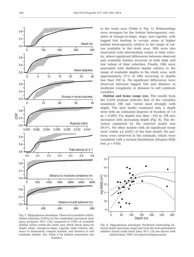
in the study area (Table 4, Fig. 7). Relationshipswere strongest for the habitat heterogeneity vari-ables of change-in-slope, slope, and rugosity, withtagged fish tending to occupy areas of higherhabitat heterogeneity relative to the range of val-ues available in the study area. HRs were alsoassociated with interme diate values of tidal veloc-ity, where significant differences between observedand available habitat occurred at both high andlow values of tidal velocities. Finally, HRs wereassociated with shallower depths relative to therange of available depths in the study area, withapproximately 75% of HRs occurring in depthsless than 100 m. No significant differences wereobserved between tagged fish and distance tomoderate complexity or distance to soft substratevariables.
Habitat and home range size. The results fromthe GAM analysis indicate that of the variablesexamined, HR size varied most strongly withdepth. The best model contained only a depthterm with an estimated degrees of freedom of 1.8(p = 0.007). For depths less than ~150 m, HR sizeincreased with increasing depth (Fig. 8). The de -viance explained by the selected model was30.0%. No other models with all significant termswere within ±2 ΔAICc of the best model. No pat-terns were observed in the residuals, which wereconsistent with a normal distribution (Shapiro-Wilktest, p = 0.65).
242
Fig. 7. Hippoglossus stenolepis. Observed cumulative distri-bution functions (CDFs) for the residential movement state(gray polygons: 95% CIs) compared to CDFs of availablehabitat values within the study area (thick black lines) fordepth, slope, change-in-slope, rugosity, tidal velocity, dis-tance to moderately complex habitat, and distance to softsubstrate habitat. See Table 4 for habitat association test
statistics
0 50 100 150 200 250 300
9
10
11
12
13
14
15
Depth (m)
log
(NS
D) (
m2 )
Fig. 8. Hippoglossus stenolepis. Predicted relationship be-tween depth and home range size from the best generalizedadditive model (solid black line); 95% CIs are shown with
dashed lines. NSD: net squared displacement
Nielsen et al.: Movement of Pacific halibut in a Marine Protected Area
DISCUSSION
Although halibut are large-bodied fish capableof moving thousands of kilometers during winterspawn ing migrations (Skud 1977, Loher & Seitz2006), our results suggests that limited dispersion atvery small spatial scales may be a common phenom-enon for adult female halibut in Glacier Bay duringthe summer and into the fall. The residential move-ment state was demonstrated by the majority (27 of43) of the fish tagged in this study. The HR dispersalpattern (which consists of residential movement inthe vicinity of the release location throughout theobservation period) was also the most frequentlyobserved dispersal pattern (n = 17) among the 32 ind.for which dispersal patterns could be determined.Although fish that exhibited the dispersive move-ment state moved more broadly around the studyarea, these movements were still relatively small(<20 km) compared to the distances moved duringwinter migrations.
Fish that were never relocated or were re locatedtoo infrequently to characterize their movement pat-terns (11 of 43 fish) may have exhibited a moremobile movement pattern and thus moved out of thestudy area quickly. In this case, they could havemoved to areas within Glacier Bay that were notmonitored during acoustic surveys or they couldhave left the interior waters of Glacier Bay entirely.Alternatively, they may have been captured in com-mercial harvests that were occurring in Glacier Bay,experienced mortality, or the tag could have beenshed or ceased to function.
Movement states
Telemetry records often document different behav-iors among individuals that are driven by differentmovement ‘states’ (Blackwell 1997, Morales et al.2004). For example, a period of intensive foragingmay result in a movement state with little net dis-placement, while a period of migration may result ina movement state with relatively large net displace-ment. Typically, ecologists are interested in the spa-tial and temporal scales of these movement states, aswell as habitat attributes with which they may beassociated (Papworth et al. 2012).
The 2 movement states, residential and dispersive,that tagged fish exhibited during the summer and falldiffered in terms of scale, duration, and potential fordispersion. The residential movement state was asso-ciated with average movement scales of <1 km for
several months at a time and a sustained, non- random lack of dispersion. In contrast, the dispersivemovement state was characterized by greater spatialscales (approx. 10 km), shorter temporal durations(<1 mo), and likely contained a mix of random anddirected movement.
Because tracking occurred during the summer for-aging season, and large adult halibut have few pred-ators, these 2 movement states could reflect differentunderlying foraging strategies. Both ‘sit-and-wait’ambush and active searching are common foragingtactics for flatfish species (Gibson 2005). The residen-tial movement pattern could be driven by a sit-and-wait tactic, which would require little movement inareas where prey is delivered to the fish. Based onlaboratory studies, a closely related congener Atlan -tic halibut Hippoglossus hippoglossus is thought tobe an ambush predator that employs a sit-and-waitfeeding tactic (Haaker 1975, Nilsson et al. 2010).Other flatfish such as summer flounder Paralichthysdentatus have been observed to employ a variety offoraging tactics — including ambush and active pur-suit — that change with prey type (Staudinger &Juanes 2010). Thus, switching between the 2 move-ment states may occur in conjunction with changes inthe type, abundance, distribution, and mobility ofprey species (see Nakano et al. 1999). However, thedispersive movement pattern could also include fishthat are moving in a directed manner from one feed-ing location to another.
Caveats. It is important to emphasize that the datapresented in this study are inherently positive andbiased toward the observation of the residentialmovement state. The experimental design employedin this study, which featured searching for taggedfish in the vicinity of their last known location,resulted in a much better characterization of the res-idential movement state compared to the dispersivemovement state. The tracking procedure was effec-tive for locating tagged fish that were occupyingHRs, as the detection range for the acoustic tags (upto 2 km) was larger than the scale of most HRs. How-ever due to the difficulty of tracking more mobile fishfor long time periods in the large study area, it islikely that the dispersive movement state occurredmore frequently than was observed and its spatialextent was not fully characterized. Although detec-tion ability was adequate for characterizing the resi-dential state throughout the study, changes in tagsize and frequency (Table S1) could have improvedthe detection of fish in the dispersive movement stateas the study progressed. It is likely that the largestmovement observed (18 km) probably reflects a prac-
243
Mar Ecol Prog Ser 517: 229–250, 2014
tical limit for the area searched during this study, somovements beyond that would have a low probabil-ity of detection.
Although it is possible that unknown tagging ef -fects may have affected the behavior of tagged hal-ibut, we feel that tagging effects are unlikely to haveaffected the scale and nature of halibut movementreported in this study for several reasons. (1) A long-term laboratory study of both internal and externalarchival tag attachment suggests that both types ofattachment are well-tolerated by halibut and do notresult in changes in behavior compared to controls(Loher & Rensmeyer 2011). (2) The tags were smallrelative to the size of the fish (average = 0.1%, maxi-mum = 0.4%). (3) Pacific halibut fitted with muchlarger pop-up satellite tags have been observed tomove more than 1000 km (Loher & Seitz 2006). (4) Wefound no statistical relationships between fish size ortag:body size ratio and maximum displacement, andno relationship between maximum displacement andtag size (small or large) or type of attachment (inter-nal or external).
Individual dispersal patterns
Non-random dispersal patterns: home range andsite fidelity. The majority of tagged fish in this studyexhibited distinctly non-random individual dispersalpatterns that were dominated by HR, but also in -cluded temporary long-distance forays followed byreturn to previously occupied locations and shiftingof HRs to new locations. The prominence of the HRdispersal pattern suggests that regular use of rela-tively small areas could be a common phenomenonduring summer. Several acoustic telemetry studieshave demonstrated summer HR behavior for otherflatfish species such as adult English sole Parophrysvetulus (S. O’Neill pers. comm.) and juvenile Califor-nia halibut Paralichthys californicus (Espasandin2012) that occurs at scales <1 km. Because some hal-ibut shifted locations for HR behavior, it is possiblethat some fish may switch HR locations depending onchanges in prey distribution and abundance and thusmay not have fidelity to specific locations.
However, multiple observations of tagged fishreturning to within several hundred meters of pre -viously occupied locations following larger-scalemovements (e.g. 10 km distance, 1 mo duration) sug-gests that some halibut do have SF to specific loca-tions (as defined by Giuggioli & Bartumeus 2012).The SF dispersal pattern was obser ved for 7 of 43 fish(including 1 fish, ID#5, that was assigned to the SHR
dispersal pattern). It is also possible that temporarydepartures from HRs were not detected due to theirregular nature of the tracking trips and the diffi-culty of relocating wide-ranging fish. In that case,subsequent relocation of these same individuals atpreviously occupied locations would indicate intra-annual SF to established HRs. Therefore intra-annualSF may be a key feature of adult female halibutmovement patterns in Glacier Bay during the sum-mer and fall.
The study has also provided some evidence forinterannual SF for halibut in Glacier Bay. Of the 4 fishreleased in November, 3 inhabited HRs at theirrelease locations the following summer. Whether ornot these fish left Glacier Bay during winter spawn-ing migrations is unknown, but 2 of these fish wereobserved at different locations within the park fol-lowing tagging (thus demonstrating an SF dispersalpattern).
These results complement previous observations ofSF for Pacific halibut from a pop-up satellite archivaltag (PSAT) study and provide further details on thescales at which it may occur. Approx. 80% of sum-mer-to-summer PSAT pop-up locations (n = 25) werelocated within 20 km of release locations after 1 yr atliberty (Loher 2008). Most (75%) of these fish hadreturned to the release location following migrationsto deeper water in the Gulf of Alaska during winter,presumably to spawn. Although the displacement fromthe release locations from the PSAT study matchesthe scale of the dispersive movement state observedin this study, the demonstrated ability of fish in thecurrent study to return to within a few hundredmeters of their original locations after undertakingforays indicates that SF for Pacific halibut likelyoccurs at much finer spatial scales than can bedetected using PSATs. SF has also been observed formany other flatfish species (Hun ter et al. 2003, Sol-mundsson et al. 2005, Sackett et al. 2008, Dando2011, Moser et al. 2013).
Random movement: diffusion. Although the majo -rity of the fish in this study displayed non-randommovement patterns associated with an overall lack ofdispersal during summer, some fish did appear tohave more mobile movement patterns. The randommovement dispersal pattern demonstrated by a smallproportion of tagged halibut suggests that some hal-ibut do not establish HRs, but may instead move ran-domly throughout summer foraging areas. The rateof diffusion associated with random movement in thisstudy, 0.9 km2 d−1, is comparable to diffusion ratesestimated for other flatfish species such as Baltic Seaturbot Psetta maxima (Florin & Franzén 2010) and
244
Nielsen et al.: Movement of Pacific halibut in a Marine Protected Area
winter flounder Pseudopleuronectes ameri canus(Saila 1961) based on results derived from conven-tional tag recaptures. Therefore, random movementappears to be another common behavior of Pleu-ronectiformes species, likely as a foraging tactic.However, sample sizes were low for this dispersalpattern, so results should be interpreted with caution.For example, these fish could also have been de -tected during temporary forays to or from HRs inunknown locations.
A large-scale summer-to-summer PIT tag study of67000 halibut provided similar observations of bothsedentary and mobile movement patterns for adulthalibut that occurred over larger scales in space andtime. Fish tagged during 2003 and 2004 had notmixed completely with the population by 2006 to2009 (Webster et al. 2013) and as of 2008, 86% of132 tags recaptured by annual survey vessels werecaught at the same survey station where they werereleased (Loher 2008). Survey stations were locatedon an 18.5 km grid, which matches the approximatescale of the dispersive movement state observed inGlacier Bay. These observations support the pres-ence of a long-term sedentary movement pattern foradult fish. On the other hand, the probability forlarge-scale movement between management unitsfor large (e.g. 130 cm) fish was close to 20% forsome units (Webster et al. 2013), which suggeststhat a more mobile movement pattern with agreater potential for dispersal also exists for adulthalibut. In ad dition to the 4 fish that exhibited therandom dispersal pattern in our study, it is possiblethat some of the 11 fish that were rarely or neverdetected had more mobile movement patterns. Inthat case, the pro portion of tagged fish with moremobile patterns would range from a minimum of9% (4 of 43) to a maximum of 35% (15 of 43),assuming no mortality, tag loss, or undetected HRbehavior at unknown locations within Glacier Bayhad occurred.
Caveats. Our use of a model selection framework tolink observed patterns of NSD vs. time to theoreticalmodels of dispersal represents a promising approachfor identifying and quantifying fish movement pat-terns in terms of ecological phenomena such as HRoccupation, foraging, and migration. This analysismethod is appropriate for data collected at irregularintervals because the analysis is based on positiveobservations of NSD at a given point in time. How-ever, due to the small sample sizes obtained for fishwith more mobile movement patterns in this study,the results for dispersal patterns other than HRshould be viewed as providing a pre liminary under-
standing of the types of behavior and spatial scalesof movement that fish may demonstrate during summer.
Habitat relationships
The habitat associations observed for tagged fishmay be related to a tendency for tagged fish to oc -cupy a specific benthic habitat type in Glacier Bay.Three regions composed of different combinations ofdepth, tidal velocity, substrate type, and communitycomposition exist in Glacier Bay (Etherington et al.2007a). The mouth and lower portions of Glacier Bayconsist of a large, flat, shallow (50 m), high-currentarea with sand and cobble substrate associated witha community of horse mussels, scallops, and seaurchins. In contrast, the central and northern portionsof the bay are composed primarily of deep fjords (toapprox. 450 m) with muddy substrates (Fig. S4) andwere associated with Tanner crab (Chionoecetesbairdi), shrimp, and flatfish species. However, themajority of fish in this study were tagged and trackedin a transition zone between these 2 areas that ischaracterized by intermediate depths, intermediatelevels of tidal velocity, mixed cobble/soft sediment,and intermediate to high levels of habitat complexity.This region is also occupied by Pacific herring (Clu-pea palasii), Pacific cod (Gadus macrocephalus),walleye pollock (Gadus chalcogrammus), rockfishes(Sebastes spp.), and other common prey items forhalibut (Best & St-Pierre 1986, Etherington et al.2007a, Moukhametov et al. 2008, Renner et al. 2012).This transition area is also a highly productive frontwhere well-mixed water from the mouth of the baymeets nutrient-rich stratified waters from the fjords(Etherington et al. 2007b).
Significant associations between the residentialmovement state and measures of habitat heteroge -neity (change-in-slope, rugosity) and tidal velocitymay also be related to a sit-and-wait foraging strat-egy. For example, complex habitat can aid conceal-ment during ambush and tides may deliver pelagicprey (see Beaudreau & Essington 2011) to ambushpredators. The strongest habitat association obser -ved was for the change-in-slope variable, which re -presents interfaces between shallow and steepslopes as well as areas where depth is frequentlychanging. Tagged halibut tended to be found in closeproximity to high values of the change-in-slope vari-able where glacial features such as moraines and icescours interface with large expanses of flat, homoge-neous terrain in the lower portion of Glacier Bay
245
Mar Ecol Prog Ser 517: 229–250, 2014
(Fig. S5). Associations with interfaces between differ-ent habitat types have been observed for other fishspecies such as the barred sand bass Paralabraxnebu lifer which inhabited interfaces between rockyreefs used for hunting and adjacent soft-sedimenthabitats used for resting or refuge (Mason & Lowe2010). Although flatfishes are often associated withsoft sediments related to their tendency to bury insediments (Gibson 2005), no significant habitat asso-ciation with distance to soft substrate habitats wasobserved here, a result that could be related to theabundance of soft sediment in the study area or areduced tendency to bury in sediment for adult fishcompared to juveniles.
Of the environmental and biological explanatoryvariables examined, only depth was significantly re -lated to HR size. Increased scales of movement indeeper areas could reflect differences in prey type orprey densities compared to shallow areas (i.e. transi-tion region communities compared to deep fjord bot-tom communities, as discussed above). A positiverelationship with depth has also been ob served fortemperate reef-associated fishes, where species thatoccupy deeper depths tend to have larger ranges ofmovement than those that occur at shallower depths(Freiwald 2012). An increase in telemetry error withdepth could confound the relationship betweendepth and HR size; however, the expected telemetryerror is still small (100 m) relative to the distancesmoved in the larger HRs (1 to 2 km). Note that the95% CIs reported for the GAM do not include errorsassociated with uncertainty of position related todepth. Because this model explained only 30% of thevariance, HR is probably affected by variables thatwere either not measured or occurred at differentscales in space or time. For example, the movementsof many fish species are known to be related to tidalpatterns on a daily basis (Tolimieri et al. 2009), so theuse of time-and-depth averaged tidal velocity in thisstudy may have been too coarse to detect relation-ships with tide. Although positive relationships be -tween fish length and HR size have been previouslyreported (Kramer & Chapman 1999), we found thatHR size was not related to fish size in this study.However the size distribution of the fish tagged inthis study was relatively homogeneous (Fig. S1), sothis result could also be related to low numbers ofvery small or very large fish. Finally, HR size did notchange over time based on the lack of significance ofthe year variable. This result implies a stability of HRscales over time as well as a lack of effect of changingtag types (frequency, size, longevity, attachmentmethod) as the study evolved (Table S2). Recent
fieldwork by the authors (J. K. Nielsen & A. C. Seitzunpubl. data), where 15 adult female halibut weretracked for 2 mo in Glacier Bay, has provided inde-pendent confirmation of the scale and dominance ofthe residential movement pattern during summer.
Implications for MPAs and spatial fisheries management
Determining fish movement scales relative to MPAsize is one of the most important aspects of MPA de -sign (Gruss et al. 2011, Saarman et al. 2013). Scales ofboth residential and dispersive movement stateswere smaller than the scale of the Glacier Bay MPA,and most tagged fish were detected regularly insidethe MPA boundary. Thus, Glacier Bay is likely toencompass the majority of movements of individualadult female Pacific halibut during the summer andfall. Retention of halibut within Glacier Bay may beencouraged by the enclosed nature of the bay, avail-ability of heterogeneous habitat with which taggedhalibut were associated, and the productivity of itswaters. Glacier Bay would therefore be ex pec ted toserve as a refuge from commercial harvest after thephase-out of commercial fisheries in the park is com-pleted (estimated by the National Park Service tooccur sometime between 2040 and 2050). However,understanding the potential for specific benefits ofGlacier Bay as an MPA such as change in size struc-ture or abundance (Taggart et al. 2004) will requiremore information on (1) large-scale movement pat-terns of halibut over yearly timescales, as fish couldbe vulnerable to commercial fishing during migra-tions from summer foraging locations to winterspawning locations outside of Glacier Bay, and (2)the effect of ongoing charter and unguided sportfishing within the park that will continue after com-mercial fishing is phased out.
In addition to insights into the potential utility ofGlacier Bay as an MPA, this study has also yielded in-formation that may be useful for design of MPAs orspatial management in general for halibut. The fre-quent observations of non-random dispersal patternssuch as HR and SF are strikingly similar to dispersalpatterns observed for other temper ate reef-associatedfishes such as lingcod (Ophiodon elongatus) andsome rockfish species (Matthews 1990, 1992, Pearcy1992, Starr et al. 2004, Tolimieri et al. 2009, Beau-dreau & Essington 2011). Lingcod, yellowtail rockfish(Sebastes flavidus), blue rockfish (Sebastes mystinus),and California scorpionfish (Scorpaena guttata) werefound to exhibit non-dispersive movement at spatial
246
Nielsen et al.: Movement of Pacific halibut in a Marine Protected Area
scales that were similar to tagged halibut in this study(Freiwald 2012, his Supplement 1, Fig. S1). Benefitssuch as increases in biomass and egg productionhave been observed for multiple temperate reef fishspecies within MPAs in California (Tetreault & Am-brose 2007). Movement patterns and scales for adultfemale lingcod tagged in a small MPA near Sitka,Alaska, which were very similar to those of the adultfemale halibut tagged in our study, suggest thatMPAs may facilitate in creased egg production throughprotection of lingcod brood stock (Starr et al. 2004).Our research suggests that MPAs may also providesome degree of protection for Pacific halibut broodstock, and therefore potential enhancement of eggproduction, based on observations of HR and SF dur-ing the summer and fall. The effectiveness of suchMPAs would then depend on the timing of winterspawning migrations, which may occur just beforeand/or after the commercial fishing season (Loher2011), as well as the proportion of adult females thatundertake annual spawning migrations (Loher &Seitz 2008). As the estimated total biomass of Pacifichalibut in the eastern North Pacific Ocean has de-clined by 50% between 1996 and 2013 and the major-ity of fish captured in the commercial fishery are fe-males (Stewart et al. 2013), additional time-areaclosures in areas where large females are found inhigh abundance could provide some measure of pro-tection during periods of declining stock abundance.
However, additional research will be required todetermine the extent to which the movement scalesand habitat associations observed in Glacier Bay, arelatively enclosed fjord estuary, may be applicableto other marine environments that occur throughoutthe range of halibut distribution. For example, limitedmovement within fjords has been observed for At-lantic halibut (Seitz et al. 2014) and Atlantic cod(Hedger et al. 2011). Movement scales may also berelated to the availability of complex habitat and highrelief areas in a given location (Matthews 1990, Beau-dreau & Essington 2011). Our results indicate that inGlacier Bay, scales of movement tend to be smaller inshallow (<100 m) areas with heterogeneous topogra-phy and complex habitat compared to deep, flat areaswith low levels of habitat complexity. Thus, althoughsome locations are likely to be more effective thanothers at retaining the movements of halibut per unitarea, more research on halibut movement scales indifferent habitat types and geographic regions isneeded to determine how much of the sedentarymovement patterns observed in this study are due to(1) fjord topography, (2) the presence of complexhabitat, or (3) inherent behavior of adult halibut.
Finally, the existence of fine-scale SF for some pro-portion of reproductive females has implications fordepletion of mature female fish at local scales.Although the phenomenon of local depletion forPacific halibut has not been explicitly documen ted,some evidence from a variety of sources suggeststhat it may be of concern. For example, declines incommercial catch per unit effort near the PribilofIslands occurred in conjunction with concentratedlocal fishing effort (Hare 2005). Localized declineshave also been observed near populated areas,where intense charter and sport fishing effort occurs(Trumble et al. 1991). Our findings of HR behaviorcombined with SF and the ability to return to previ-ously occupied areas suggest a potential mechanismby which Pacific halibut could be vulnerable to localdepletion. However, before the potential for localdepletion can be characterized, broad geographic-scale dispersal processes, population connectivity,and spatial structure during other life history phases,such as passive planktonic larval drift and contranatantontogenetic migrations, must be fully assessed (Skud1977, Conners & Munro 2008).
Benefits of NSD analysis methods
Our use of NSD analyses to describe and quantifymovement patterns and scales is a novel, robust ap -proach that can be applied to irregular datasets com-monly collected for fishes. Using the analysis of dis-persal patterns, telemetry records for tagged fish canbe analyzed in the context of movement ecology andpotential for dispersal, rather than focusing on thesize or location of an area inhabited by the fish. Themixed-effects model framework allows the descrip-tion of inherent individual variability, as well as bor-rowing ‘strength’ from individuals with more obser-vations. Information on movement characteristics isprovided in formats such as diffusion rates or HRscales that can be easily used to simulate movementpaths for use in other studies. For ex ample, such sim-ulations could be used to estimate energy budgetsduring residential versus dispersive movement states.In addition, it provides a way to compare results be -tween acoustic and conventional tagging studies. Forexample, diffusion coefficients have been calculatedfor American lobsters using the slope of NSD vs. timefrom conventional tag recovery data (den Heyer et al.2009). Thus, this method may provide a way to lever-age the detailed information provided by acousticstudies with the larger sample sizes available fromconventional tagging studies.
247
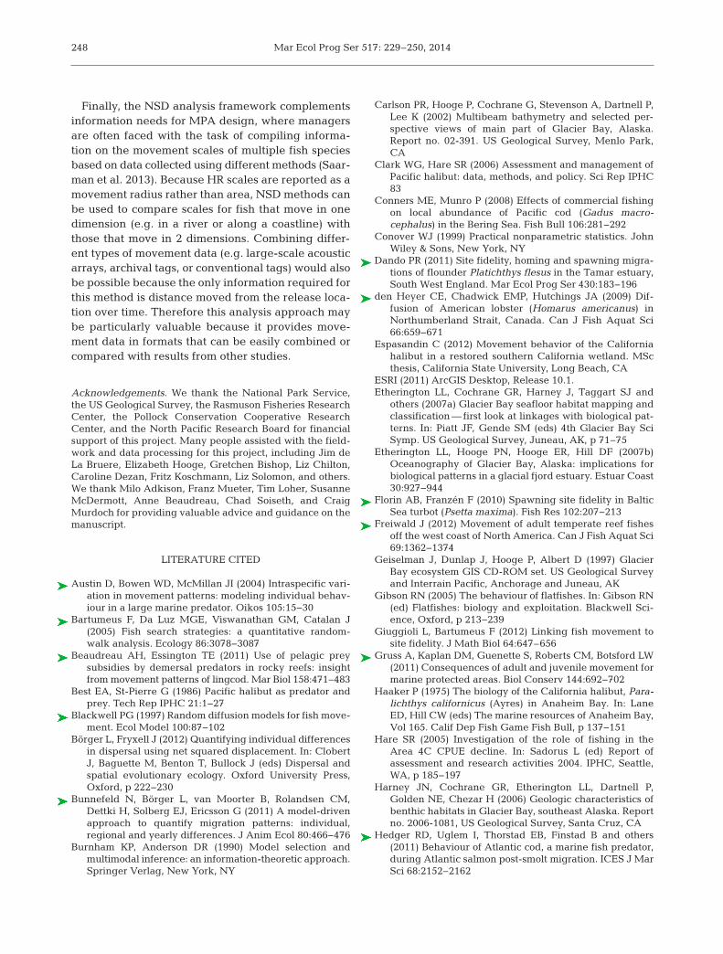
Mar Ecol Prog Ser 517: 229–250, 2014
Finally, the NSD analysis framework complementsinformation needs for MPA design, where managersare often faced with the task of compiling informa-tion on the movement scales of multiple fish speciesbased on data collected using different methods (Saar -man et al. 2013). Because HR scales are reported as amovement radius rather than area, NSD methods canbe used to compare scales for fish that move in onedimension (e.g. in a river or along a coastline) withthose that move in 2 dimensions. Combining differ-ent types of movement data (e.g. large-scale acousticarrays, archival tags, or conventional tags) would alsobe possible because the only information required forthis method is distance moved from the release loca-tion over time. Therefore this analysis approach maybe particularly valuable because it provides move-ment data in formats that can be easily combined orcompared with results from other studies.
Acknowledgements. We thank the National Park Service,the US Geological Survey, the Rasmuson Fisheries ResearchCenter, the Pollock Conservation Co operative ResearchCenter, and the North Pacific Research Board for financialsupport of this project. Many people assisted with the field-work and data processing for this project, including Jim deLa Bruere, Elizabeth Hooge, Gretchen Bishop, Liz Chilton,Caroline Dezan, Fritz Koschmann, Liz Solomon, and others.We thank Milo Adkison, Franz Mueter, Tim Loher, SusanneMcDermott, Anne Beaudreau, Chad Soiseth, and CraigMurdoch for providing valuable advice and guidance on themanuscript.
LITERATURE CITED
Austin D, Bowen WD, McMillan JI (2004) Intraspecific vari-ation in movement patterns: modeling individual behav-iour in a large marine predator. Oikos 105: 15−30
Bartumeus F, Da Luz MGE, Viswanathan GM, Catalan J(2005) Fish search strategies: a quantitative random-walk analysis. Ecology 86: 3078−3087
Beaudreau AH, Essington TE (2011) Use of pelagic preysubsidies by demersal predators in rocky reefs: insightfrom movement patterns of lingcod. Mar Biol 158: 471−483
Best EA, St-Pierre G (1986) Pacific halibut as predator andprey. Tech Rep IPHC 21: 1−27
Blackwell PG (1997) Random diffusion models for fish move-ment. Ecol Model 100: 87−102
Börger L, Fryxell J (2012) Quantifying individual differencesin dispersal using net squared displacement. In: ClobertJ, Baguette M, Benton T, Bullock J (eds) Dispersal andspatial evolutionary ecology. Oxford University Press,Oxford, p 222−230
Bunnefeld N, Börger L, van Moorter B, Rolandsen CM, Dettki H, Solberg EJ, Ericsson G (2011) A model-drivenapproach to quantify migration patterns: individual,regional and yearly differences. J Anim Ecol 80: 466−476
Burnham KP, Anderson DR (1990) Model selection andmulti modal inference: an information-theoretic ap proach.Springer Verlag, New York, NY
Carlson PR, Hooge P, Cochrane G, Stevenson A, Dartnell P,Lee K (2002) Multibeam bathymetry and selected per-spective views of main part of Glacier Bay, Alaska.Report no. 02-391. US Geological Survey, Menlo Park,CA
Clark WG, Hare SR (2006) Assessment and management ofPacific halibut: data, methods, and policy. Sci Rep IPHC83
Conners ME, Munro P (2008) Effects of commercial fishingon local abundance of Pacific cod (Gadus macro-cephalus) in the Bering Sea. Fish Bull 106: 281−292
Conover WJ (1999) Practical nonparametric statistics. JohnWiley & Sons, New York, NY
Dando PR (2011) Site fidelity, homing and spawning migra-tions of flounder Platichthys flesus in the Tamar estuary,South West England. Mar Ecol Prog Ser 430: 183−196
den Heyer CE, Chadwick EMP, Hutchings JA (2009) Dif -fusion of American lobster (Homarus americanus) inNorthumberland Strait, Canada. Can J Fish Aquat Sci66: 659−671
Espasandin C (2012) Movement behavior of the Californiahalibut in a restored southern California wetland. MScthesis, California State University, Long Beach, CA
ESRI (2011) ArcGIS Desktop, Release 10.1.Etherington LL, Cochrane GR, Harney J, Taggart SJ and
others (2007a) Glacier Bay seafloor habitat mapping andclassification — first look at linkages with biological pat-terns. In: Piatt JF, Gende SM (eds) 4th Glacier Bay SciSymp. US Geological Survey, Juneau, AK, p 71−75
Etherington LL, Hooge PN, Hooge ER, Hill DF (2007b)Oceanography of Glacier Bay, Alaska: implications forbiological patterns in a glacial fjord estuary. Estuar Coast30: 927−944
Florin AB, Franzén F (2010) Spawning site fidelity in BalticSea turbot (Psetta maxima). Fish Res 102: 207−213
Freiwald J (2012) Movement of adult temperate reef fishesoff the west coast of North America. Can J Fish Aquat Sci69: 1362−1374
Geiselman J, Dunlap J, Hooge P, Albert D (1997) GlacierBay ecosystem GIS CD-ROM set. US Geological Surveyand Interrain Pacific, Anchorage and Juneau, AK
Gibson RN (2005) The behaviour of flatfishes. In: Gibson RN(ed) Flatfishes: biology and exploitation. Blackwell Sci-ence, Oxford, p 213−239
Giuggioli L, Bartumeus F (2012) Linking fish movement tosite fidelity. J Math Biol 64: 647–656
Gruss A, Kaplan DM, Guenette S, Roberts CM, Botsford LW(2011) Consequences of adult and juvenile movement formarine protected areas. Biol Conserv 144: 692−702
Haaker P (1975) The biology of the California halibut, Para -lichthys californicus (Ayres) in Anaheim Bay. In: LaneED, Hill CW (eds) The marine resources of Anaheim Bay,Vol 165. Calif Dep Fish Game Fish Bull, p 137−151
Hare SR (2005) Investigation of the role of fishing in theArea 4C CPUE decline. In: Sadorus L (ed) Report ofassessment and research activities 2004. IPHC, Seattle,WA, p 185−197
Harney JN, Cochrane GR, Etherington LL, Dartnell P,Golden NE, Chezar H (2006) Geologic characteristics ofbenthic habitats in Glacier Bay, southeast Alaska. Reportno. 2006-1081, US Geological Survey, Santa Cruz, CA
Hedger RD, Uglem I, Thorstad EB, Finstad B and others(2011) Behaviour of Atlantic cod, a marine fish predator,during Atlantic salmon post-smolt migration. ICES J MarSci 68: 2152−2162
248

Nielsen et al.: Movement of Pacific halibut in a Marine Protected Area
Hill DF, Ciavola SJ, Etherington L, Klaar MJ (2009) Estima-tion of freshwater runoff into Glacier Bay, Alaska andincorporation into a tidal circulation model. Estuar CoastShelf Sci 82: 95−107
Hunter E, Metcalfe JD, Reynolds JD (2003) Migration routeand spawning area fidelity by North Sea plaice. Proc RSoc Lond B Biol Sci 270: 2097−2103
Jorgensen SJ, Reeb CA, Chapple TK, Anderson S and others(2010) Philopatry and migration of Pacific white sharks.Proc R Soc Lond B Biol Sci 277: 679−688
Kareiva PM, Shigesada N (1983) Analyzing insect movementas a correlated random walk. Oecologia 56: 234−238
Kramer DL, Chapman MR (1999) Implications of fish homerange size and relocation for marine reserve function.Environ Biol Fishes 55: 65−79
Loher T (2008) Homing and summer feeding site fidelity ofPacific halibut (Hippoglossus stenolepis) in the Gulf ofAlaska, established using satellite-transmitting archivaltags. Fish Res 92: 63−69
Loher T (2011) Analysis of match−mismatch between com-mercial fishing periods and spawning ecology of Pacifichalibut (Hippoglossus stenolepis), based on winter sur-veys and behavioural data from electronic archival tags.ICES J Mar Sci 68: 2240−2251
Loher T, Rensmeyer R (2011) Physiological responses ofPacific halibut, Hippoglossus stenolepis, to intracoelomicimplantation of electronic archival tags, with a review oftag implantation techniques employed in flatfishes. RevFish Biol Fish 21: 97−115
Loher T, Seitz A (2006) Seasonal migration and environmen-tal conditions of Pacific halibut Hippoglossus steno lepis,elucidated from pop-up archival transmitting (PAT) tags.Mar Ecol Prog Ser 317: 259−271
Loher T, Seitz AC (2008) Characterization of active spawn-ing season and depth for eastern Pacific halibut (Hip-poglossus stenolepis), and evidence of probable skippedspawning. J Northwest Atl Fish Sci 41: 23−36
Mason TJ, Lowe CG (2010) Home range, habitat use, andsite fidelity of barred sand bass within a southern Califor-nia marine protected area. Fish Res 106: 93−101
Matthews KR (1990) A telemetric study of the home rangesand homing routes of copper and quillback rockfishes onshallow rocky reefs. Can J Zool 68: 2243−2250
Matthews KR (1992) A telemetric study of the home rangesand homing routes of lingcod Ophiodon elongatus onshallow rocky reefs off Vancouver Island, British Colum-bia. Fish Bull 90: 784−790
Moorcroft PR, Lewis MA (2006) Mechanistic home rangeanalysis. Princeton University Press, Princeton andOxford
Morales JM, Haydon DT, Frair J, Holsinger KE, Fryxell JM(2004) Extracting more out of relocation data: buildingmovement models as mixtures of random walks. Ecology85: 2436−2445
Moser ML, Myers MS, West JE, O’Neill SM, Burke BJ (2013)English sole spawning migration and evidence for feed-ing site fidelity in Puget Sound, U.S.A., with implicationsfor contaminant exposure. Northwest Sci 87: 317−325
Moukhametov IN, Orlov AM, Leaman BM (2008) Diet ofPacific halibut (Hippoglossus stenolepis) in the north-western Pacific Ocean. Tech Rep IPHC 52
Nakano S, Fausch KD, Kitano S (1999) Flexible niche parti-tioning via a foraging mode shift: a proposed mechanismfor coexistence in stream-dwelling charrs. J Anim Ecol68: 1079−1092
Nilsson J, Kristiansen TS, Fosseidengen JE, Stien LH, FernoA, van den Bos R (2010) Learning and anticipatorybehaviour in a ‘sit-and-wait’ predator: the Atlantic halibut. Behav Processes 83: 257−266
Nouvellet P, Bacon JP, Waxman D (2009) Fundamentalinsights into the random movement of fish from a singledistance-related statistic. Am Nat 174: 506−514
Papworth SK, Bunnefeld N, Slocombe K, Milner-Gulland EJ(2012) Movement ecology of human resource users: using net squared displacement, biased random bridgesand resource utilization functions to quantify hunter andgatherer behaviour. Methods Ecol Evol 3: 584−594
Pearcy WG (1992) Movements of acoustically-tagged yel-lowtail rockfish Sebastes flavidus on Heceta bank, Ore-gon. Fish Bull 90: 726−735
Perry RI, Smith SJ (1994) Identifying habitat associations ofmarine fishes using survey data: an application to thenorthwest Atlantic. Can J Fish Aquat Sci 51: 589−602
Pinheiro J, Bates D (2000) Mixed-effects models in S and S-PLUS. Springer-Verlag, New York, NY
Renner M, Arimitsu ML, Piatt JF (2012) Structure of marinepredator and prey communities along environmentalgradients in a glaciated fjord. Can J Fish Aquat Sci 69: 2029−2045
Rogers KB, White GC (2007) Analysis of movement andhabitat use from telemetry data. In: Brown M, Guy C(eds) Analysis and interpretation of freshwater fish-eries data. American Fisheries Society, Bethesda, MD,p 625−676
Saarman E, Gleason M, Ugoretz J, Airamé S and others(2013) The role of science in supporting marine protectedarea network planning and design in California. OceanCoast Manag 74: 45−56
Sackett DK, Able KW, Grothues TM (2008) Habitat dynam-ics of summer flounder Paralichthys dentatus within ashallow USA estuary, based on multiple approachesusing acoustic telemetry. Mar Ecol Prog Ser 364: 199−212
Saila SB (1961) A study of winter flounder movements. Lim-nol Oceanogr 6: 292−298
Seitz AC, Loher T, Norcross BL, Nielsen JL (2011) Dispersaland behavior of Pacific halibut Hippoglossus stenolepisin the Bering Sea and Aleutian Islands region. Aquat Biol12: 225−239
Seitz AC, Michalsen K, Nielsen JL, Evans MD (2014) Evi-dence of fjord spawning by southern Norwegian Atlantichalibut (Hippoglossus hippoglossus). ICES J Mar Sci 71:142–147
Singh NJ, Borger L, Dettki H, Bunnefeld N, Ericsson G(2012) From migration to nomadism: movement variabil-ity in a northern ungulate across its latitudinal range.Ecol Appl 22: 2007−2020
Skud BE (1977) Drift, migration, and intermingling of Pacifichalibut stocks. Sci Rep IPHC 63
Solmundsson J, Palsson J, Karlsson H (2005) Fidelity ofmature Icelandic plaice (Pleuronectes platessa) to spaw -ning and feeding grounds. ICES J Mar Sci 62: 189−200
Starr RM, O’Connell V, Ralston S (2004) Movements of ling-cod (Ophiodon elongatus) in southeast Alaska: potentialfor increased conservation and yield from marine re -serves. Can J Fish Aquat Sci 61: 1083−1094
Staudinger MD, Juanes F (2010) Feeding tactics of a behav-iorally plastic predator, summer flounder (Paralichthysdentatus). J Sea Res 64: 68−75
Stewart IJ, Leaman BM, Martell S, Webster RA (2013)Assessment of the Pacific halibut stock at the end of
249
Mar Ecol Prog Ser 517: 229–250, 2014
2012. In: Sadorus L (ed) Report of assessment andresearch activities 2012. IPHC, Seattle, WA, p 93−186
Taggart SJ, Shirley TC, O’Clair CE, Mondragon J (2004)Dramatic increase in the relative abundance of largemale dungeness crabs Cancer magister following closureof commercial fishing in Glacier Bay, Alaska. Am FishSoc Symp 42: 243−253
Tetreault I, Ambrose RF (2007) Temperate marine reservesenhance targeted but not untargeted fishes in multipleno-take MPAs. Ecol Appl 17: 2251−2267
Tolimieri N, Andrews K, Williams G, Katz S, Levin PS (2009)Home range size and patterns of space use by lingcod,copper rockfish and quillback rockfish in relation to dieland tidal cycles. Mar Ecol Prog Ser 380: 229−243
Trumble RJ, St-Pierre G, McGregor IR (1991) Evaluation ofPacific halibut management for regulatory area 2A. SciRep IPHC 74
Turchin P (1998) Quantitative analysis of movement: meas-uring and modeling population redistribution in fish andplants. Sinauer Associates, Sunderland, MA
Valero JL, Webster RA (2012) Current understanding ofPacific halibut migration patterns. In: Sadorus L (ed)Report of assessment and research activities 2011. IPHC,Seattle, WA, p 341−379
Webster RA, Stewart IJ (2014) Apportionment and regula-tory area harvest calculations. In: Sadorus L (ed) Reportof assessment and research activities 2013. IPHC, Seat-tle, WA, p 197−216
Webster RA, Clark WG, Leaman BM, Forsberg JE (2013)Pacific halibut on the move: a renewed understanding ofadult migration from a coastwide tagging study. Can JFish Aquat Sci 70: 642−653
Wood SN (2006) Generalized Additive Models: an introduc-tion with R. Chapman & Hall/CRC, Boca Raton, FL
Wright DJ, Pendleton M, Boulware J, Walbridge S, Gerlt B,Eslinger D, Sampson D, Huntley E (2012) ArcGIS BenthicTerrain Modeler (BTM), v. 3.0. Environmental SystemsResearch Institute, NOAA Coastal Services Center, Mas-sachusetts Office of Coastal Zone Management. http://esriurl.com/5754
250
Editorial responsibility: Nicholas Tolimieri, Seattle, Washington, USA
Submitted: March 6, 2014; Accepted: September 12, 2014Proofs received from author(s): December 3, 2014