A characterization of the strong law of largenumbers for Bernoulli sequencesLUÍSA BORSATO1, EDUARDO HORTA2,* and RAFAEL RIGÃO SOUZA2,†

1Institute of Mathematics and Statistics, Universidade de São Paulo, São Paulo, Brazil.E-mail: luisabborsato@gmail.com2Institute of Mathematics and Statistics, Universidade Federal do Rio Grande do Sul, Porto Alegre, Brazil.E-mail: *eduardo.horta@ufrgs.br; †rafars@mat.ufrgs.br

The law of large numbers is one of the most fundamental results in Probability Theory. In the case of independentsequences, there are some known characterizations; for instance, in the independent and identically distributedsetting it is known that the law of large numbers is equivalent to integrability. In the case of dependent sequences,there are no known general characterizations — to the best of our knowledge. We provide such a characterizationfor identically distributed Bernoulli sequences in terms of a product disintegration.

Keywords: law of large numbers, random measure, disintegration, conditional independence.

1. Introduction

It is somewhat intuitive to most people1 that if a coin is thrown independently a large number of times,then the observed proportion of heads should not be far from the parameter of unbalancedness θ ∈ [0,1](this quantity being understood as representing the probability, or ‘chance’, of observing heads in anyone individual throw). In the Theory of Probability, the law of large numbers supports, generalizes andalso provides a precise mathematical meaning to this intuition — an intuition which can be traced backat least to Cardano’s 16th-century Liber de ludo aleae [3]. In his 1713 treatise Ars Conjectandi, JacobBernoulli gave the first proof of the fact that (in modern notation) if X is a Binomial random variablewith parameters n ∈ N and 0 ≤ p ≤ 1, then one has the inequality P(|n−1X − p| > ε) ≤ (1 + c)−1,provided n is large enough, where ε and c are arbitrarily prescribed positive constants [1]. This is atypical weak law statement — although it was not until the time of Poisson that the name “loi desgrands nombres” was coined [11, p.7]. See [13, 14] for a compelling historical perspective on the lawof large numbers, a history which culminated in ‘the’ strong law for independent and identically dis-tributed sequences, according to which the almost sure convergence of the sequence of sample meansto the (common) expected value is equivalent to integrability. Also, still in the context of independentsequences, we highlight the importance of Kolmogorov’s strong law for independent sequences whosepartial sums have variances satisfying a summability condition.

1One may argue that most people interpret probability — at least when it comes to coin-throwing — in a Popperian sense,i.e. seeing probability statements as utterances which quantify the physical propensity of a given outcome in a given experiment,in lieu of an epistemic view where such statements only measure the degree to which we are uncertain about said outcome[12]. To us the propensity interpretation seems adequate in the framework of coin-throwing, as it is meaningful to establish aconnection between the coin’s physical center of mass and the propensity of it landing ‘heads’ in any one given throw: recallingthat a coin throw is governed by classical (deterministic) mechanics, we could for instance let Ω denote the set of all possibleinitial conditions (angle, speed, spin, etc) and then make the requirement that the subset comprised of all initial conditions whosecorresponding outcome is ‘heads’ be a measurable set, with measure p ∈ [0,1]. Clearly such p is a function of the coin’s centerof mass.

1

arX

iv:2

008.

0031

8v1

[m

ath.

PR]

1 A

ug 2

020

2

Outside the realm of independence, things get trickier. As famously put by Michel Loève [9, p.6],“martingales, Markov dependence and stationarity are the only three dependence concepts so far iso-lated which are sufficiently general and sufficiently amenable to investigation, yet with a great numberof deep properties”. The contemporary probabilist would likely add uncorrelatedness, m-dependence,exchangeability and mixing properties to that list. In any case, the ways through which independencemay fail to hold are manifold, and thus one might infer that dependence is too wide a concept, whichmeans we should not expect to easily obtain a characterization of the law of large numbers for depen-dent sequences. Indeed, there are many scenarios where one can give sufficient conditions under whicha law of large numbers holds for such sequences — to cite just a few examples: the weak law for pair-wise uncorrelated sequences of random variables; the strong law for mixing sequences [7, 8]; the stronglaw for exchangeable sequences [16]; some very interesting results concerning decay of correlations(see, for example, [17]) — but, to the best of our knowledge, no characterization has been providedso far2. In this paper, we provide one such characterization for sequences of identically distributedBernoulli random variables, in terms of the concept of a product disintegration. Our main result showsthat, to a certain degree, independence is an inextricable aspect of the law of large numbers.

Our conceptualization derives from — and generalizes — the notion of an exchangeable sequenceof random variables, to which we shall recall the precise definition shortly. First, let us get back toheuristics. The intuition underlying the coin-throwing situation depicted above remains essentially thesame if we assume that, before fabricating the coin, the parameter of unbalancedness will be chosen atrandom in the interval [0,1]. In this case, conditionally on the value of the randomly chosen ϑ (let us saythat the realized value is θ), the long run proportion of heads definitely ought to approach θ. The naturalfollow-up is to consider the not so evident scenario in which we choose at random (possibly distinct)parameters of unbalancedness ϑ0, . . . , ϑn, . . . and then, given a realization of these random variables(say, θ0, . . . , θn, . . . ), we fabricate distinct coins accordingly, that is, each corresponding to one of thesampled parameters of unbalancedness, and then sequentially throw them, independently from oneanother. Our main result implies that, if the sequence (ϑn) is stationary and satisfies a law of largenumbers, then the long run proportion of heads in the latter scenario will approach Eϑ0. Moreover, weshow that the converse is also true: if a stationary sequence of coin throws has the property that theproportion of heads in the first n throws approaches, with certainty, the parameter of unbalancedness,then the coin throws are conditionally independent, where the conditioning is on a sequence of randomparameters of unbalancedness satisfying themselves a law of large numbers.

As a byproduct stemming from our effort to provide a rigorous proof to Theorem 2.1, we developedthe framework of product disintegrations, which provides a model for sequences of random variablesthat are conditionally independent — but not necessarily identically distributed — thus being a gen-eralization of exchangeability. In this context, we highlight the importance of Theorem 3.7, whichconstitutes the fundamental step in proving Theorem 2.1 and also yields several examples that illus-trate applications of both mathematical and statistical interest.

The paper is organized as follows. In the next section we state our main result, Theorem 2.1, andprovide some heuristics connecting our conceptualization to the theory of exchangeable sequencesof random variables and to de Finetti’s Theorem. In section 3, we develop the theory in a slightlymore general framework, introducing the concept of a product disintegration as a generalization ofexchangeability. We then state and prove our auxiliary results, of which Theorem 2.1 is an immediatecorollary. Section 4 provides a few examples.

2It is well known that the problem can be translated — although not ipsis litteris — to the language of Ergodic Theory,and there are many characterizations of ergodicity of a dynamical system. The law of large numbers for stationary sequences isindeed implied by the Ergodic Theorem, but the converse implication does not hold in general.

A characterization of the strong LLN for Bernoulli sequences 3

2. Main result and its relation to exchangeability

We now state our main result. The proof is postponed to section 3.

Theorem 2.1. Let X := (X0,X1, . . . ) be a sequence of Bernoulli(p) random variables, where 0 ≤p≤ 1. Then one has

limn→∞

1

n

n−1∑i=0

Xi = p, almost surely (1)

if and only if there exists a sequence ϑ = (ϑ0, ϑ1, . . . ) of random variables taking values in the unitinterval such that:

1. almost surely, for all n≥ 0 and all x0, x1, . . . , xn ∈ 0,1 one has

P(X0 = x0, . . . ,Xn = xn |ϑ) =

n∏i=0

ϑxii (1− ϑi)1−xi , (2)

and2. almost surely, it holds that

limn→∞

1

n

n−1∑i=0

ϑi = p. (3)

Remark 2.2. The above theorem says that a sequence of coin throws has the property that the pro-portion of heads in the first n throws approaches, with certainty, the “parameter of unbalancedness”p ∈ [0,1] if and only if the coin throws are conditionally independent, where the conditioning is on asequence of random parameters of unbalancedness whose corresponding sequence of sample meansconverges to p. Thus, for sequences of identically distributed Bernoulli(p) random variables, the stronglaw of large numbers holds precisely when the experiment can be described as the outcome of a two-step mechanism, in which the first step encapsulates dependence and convergence of the sample means,whereas in the second step the random variables are realized in an independent manner.

The conditional independence expressed in equation (2) is closely related to the notion of exchange-ability. Recall that a sequence X := (X0,X1, . . . ) of random variables is said to be exchangeable ifffor every n≥ 1 and every permutation σ of 0, . . . , n it holds that the random vectors (X0, . . . ,Xn)and (Xσ(0), . . . ,Xσ(n)) are equal in distribution. An important characterization of exchangeability, deFinetti’s Theorem states that a necessary and sufficient condition for a sequence of random variablesto be exchangeable is that it is conditionally independent and identically distributed. To be precise,in the context of a sequence X := (X0,X1, . . . ) of Bernoulli(p) random variables, exchangeability isequivalent to existence of a random variable ϑ taking values in the unit interval such that, almost surely,for all n≥ 0 and all x0, . . . , xn ∈ 0,1 one has

P (X0 = x0, . . . ,Xn = xn |ϑ) =

n∏i=0

ϑxi(1− ϑ)1−xi . (4)

Moreover, ϑ is almost surely unique and given by ϑ = limn→∞ n−1∑n−1i=0 Xi. In fact, the above

equivalence holds with greater generality — see [6, Theorem 11.10].

4

In view of de Finetti’s Theorem, one is tempted to ask what happens when the random product mea-sure (4) characterizing exchangeable sequences — whose factors are all the same random probabilitymeasure — is substituted by an arbitrary random product measure (whose factors are not necessarilythe same). This led us to introduce the concept of a product disintegration, which we develop below,and which ultimately provided us with the framework yielding Theorem 2.1.

3. General theory and proof of Theorem 2.1We now proceed to developing a slightly more general theory — one that will lead us to Theorem 3.7,of which Theorem 2.1 is a corollary. Let us begin by establishing some terminology and notation. In allthat follows, S is a compact, metrizable space. We letM1(S) denote the set of Borel probability mea-sures on S. The former is itself a compact metrizable space when endowed with the topology of weak*convergence — according to which a sequence (µn) of probability measures converges to a givenµ ∈M1(S) if and only if

∫f(x)µn(dx)→

∫f(x)µ(dx), for each continuous function f : S → R.

In particular M1(S) admits a Borel σ-field — see Theorem A.3. If (Ω,F ,P) is a probability spaceand ξ : Ω→M1(S) is a Borel measurable mapping, we call ξ a random probability measure on S,whose value (which is a fixed probability measure) at a point ω ∈Ω we shall denote by ξω and ξ(ω, ·)interchangeably. Measb(S) denotes the space of measurable, bounded maps from S to R, and C (S)denotes the subspace of Measb(S) comprised of continuous maps from S to R. Given f ∈Measb(S)

and µ ∈M1 (S) we shall write∫f(x)µ(dx), µ (f) and f(µ) interchangeably. If ξ is a random prob-

ability measure on S, the baricenter of ξ is defined as the unique element Eξ ∈M1 (S) such that theequality

∫Ω

∫S f(x)ξω(dx)P(dω) =

∫S f(x)Eξ(dx) holds for all f ∈C (S). The baricenter Eξ is also

known as the Pettis integral of ξ with respect to P, or as the P-expectation of ξ, and its existence isguaranteed by the Riesz-Markov Theorem A.21. As usual, we write PY for the distribution of a ran-dom variable Y with values in a measurable spaceM , that is, PY (B) = P (Y ∈B), for any measurablesubset B ⊆M . In what follows N denotes the set of nonnegative integers.

Definition 3.1 (Product Disintegration). Let X := (X0,X1, . . . ) be a sequence of random variablestaking values in a compact metric space S. We say that a sequence ξ := (ξ0, ξ1, . . . ) of random proba-bility measures on S is a product disintegration ofX iff, with probability one, the equality

P [X0 ∈A0, . . . ,Xn ∈An |ξ] = ξ0 (A0) · · · ξn (An) (5)

holds for each n ∈ N and each family A0, . . . ,An of measurable subsets of S. If ξ is a stationarysequence, then we say that ξ is a stationary product disintegration.

The definition above says that, conditionally on ξ, the sequence X := (X0,X1, . . . ) is independent— or, to be more precise, that for almost all elementary outcome ω in the sample space, it holds that theconditional probability P(X ∈ · |ξ)ω is a product measure on SN. See the standard construction belowfor more details, where a justification for the terminology disintegration is provided. Also, notice thatif ξ is stationary, then clearlyX is stationary as well.

The following result is an important characterization of product disintegrations. It allows us to workwith the seemingly weaker requirement that the identity (5) hold only on a set Ω[n;A0, . . . ,An] havingP-measure 1, for each n ∈N and each family A0, . . . ,An of measurable subsets of S.

Lemma 3.2. Let X := (X0,X1, . . . ) be a sequence of random variables taking values in a compactmetric space S, and let ξ = (ξ0, ξ1, . . . ) be a sequence of random probability measures on S. Thenξ is a product disintegration of X if and only if for each n and each (n + 1)-tuple A0, . . . ,An ofmeasurable subsets of S, the equality (5) holds almost surely.

A characterization of the strong LLN for Bernoulli sequences 5

Proof. The ‘only if’ part of the statement is trivial. For the ‘if’ part, let S N denote the product σ-fieldon SN. By Lemma A.14, S N coincides with the Borel σ-field corresponding to the product topology onSN, and therefore SN is a Borel space. By Theorem A.12, there exists an event Ω∗ ⊆Ω with P(Ω∗) = 1such thatA 7→ P(X ∈A |ξ)ω is a probability measure on S N for each ω ∈Ω∗.

Now let C := Ak : k ∈N be a countable collection of sets of the formAk =Bk0 × · · · ×Bkn(k) ×S×· · · which generates S N (see Corollary A.15). By assumption, for each k there is an event Ωk ⊆Ωwith P(Ωk) = 1 such that P(X ∈ Ak |ξ)ω = ξω0 (Bk0 ) · · · ξωn(k)(B

kn(k)) holds for ω ∈ Ωk. Thus, for

ω ∈ Ω′ := (⋂∞k=0Ak) ∩ Ω∗, with P(Ω′) = 1, the probability measures P(X ∈ · |ξ)ω and

∏∞n=0 ξ

ωn

agree on a π-system which generates S N, and therefore they agree on S N. This establishes the statedresult.

Now we prove that product disintegrations always exist:

Lemma 3.3. Any sequence X := (X0,X1, . . . ) of S-valued random variables admits a product dis-integration.

Proof. For n ∈N and ω ∈Ω, let ξωn = δXn(ω), where δx is the Dirac measure at x ∈ S. Now fix n ∈Nand let A0, . . . ,An be measurable subsets of S. We first prove that the map

ω 7→ ξω0 (A0) · · · ξωn (An)≡ I[X0∈A0,...,Xn∈An] (ω) (6)

is σ (ξ)-measurable and integrable: by Theorem A.1, the maps fAi: M1(S)→R defined by fAi

(µ) :=µ(Ai), are measurable and thus, by the Doob-Dynkin Lemma A.20, the map ω 7→ ξωi (Ai) = fAi

ξi(ω) is measurable with respect to σ(ξi)⊆ σ(ξ). Thus (6) defines a σ(ξ)-measurable map, as stated.Moreover, for B ∈ σ (ξ) we have

Eξ0 (A0) · · · ξn (An) IB= EI[X0∈A0,...,Xn∈An,B]

= PX0 ∈A0, . . . ,Xn ∈An,B ,

and therefore ξ0 (A0) · · · ξn (An) is a version of P [X0 ∈A0, . . . ,Xn ∈An |ξ]. Now it is only a matterof applying Lemma 3.2.

We shall call the sequence δ =(δX0

, δX1, . . .

)appearing in the above lemma the canonical prod-

uct disintegration of X . Notice, in particular, that product disintegrations are not unique (see Exam-ple 4.1). Also, it is clear that stationarity ofX entails stationarity of δ.

We now argue that, without loss of generality, one can take the underlying probability space Ω tobe the compact metric space SN ⊗M1(S)N, endowed with its Borel σ-field F , and equipped with theprobability measure defined, for Borel subsetsA⊆ SN andB ⊆M1(S)N, by

P(A×B) =

∫Bρ(λ,A)Q(dλ) (7)

where Q is a probability measure defined on M1(S)N (that is, Q ∈M1(M1(S)N)) and

ρ(λ,A) :=(∏

i∈Nλi

)(A), λ ∈M1(S)N, A⊆ SN measurable.

In this construction, the random variables X and ξ can be defined as projections by putting, for ω =(x,λ) ∈Ω,X(ω) := x and ξ(ω) := λ, where x= (x0, x1, . . . ) and λ= (λ0, λ1, . . . ). The next lemmaensures that, in the probability space (Ω,F ,P), indeed ξ is a product disintegration ofX , with Pξ =Q.For convenience, we shall call this the standard construction.

6

Lemma 3.4. ρ is a probability kernel from M1(S)N to SN.

Proof. It is sufficient to prove that the map λ 7→ ρ(λ, ·) ≡∏i∈N λi from M1(S)N to M1(SN) is

measurable. Let (λn) be a sequence inM1(S)N, i.e., for each n,λn = (λn0 , λn1 , . . . ) with λni ∈M1(S),

for each i, such that limn→∞λn = λ = (λ0, λ1, . . . ) ∈M1(S)N; that is, limn→+∞ λni = λi, for alli. Also, let A = A0 × A1 × · · · × AL × S × S × . . . be an open set in SN. Since limn→+∞ λni =λi, we know, by the Portmanteau Theorem, that lim infn→+∞ λni (Ai) ≥ λi(Ai). Now, ρ (λn,A) =(∏

j∈N λnj

)(A) =

∏Lj=0 λ

nj (Aj). This implies

lim infn→+∞

ρ (λn,A) = lim infn→+∞

L∏j=0

λnj (Aj) =

L∏j=0

lim infn→+∞

λnj (Aj)≥L∏j=0

λj(Aj) = ρ (λ,A) ,

which proves that λ 7→ ρ(λ, ·) is continuous and, a fortiori, measurable.

Interestingly, the standard construction evinces the fact that the joint law of a sequence of randomvariables with values in S can always be written as the baricenter of a random product measure on SN.Indeed, as product disintegrations always exist (Lemma 3.3), if we let X = (X0,X1, . . . ) be such asequence (and seeingX as a SN-valued random variable) with product disintegration ξ = (ξ0, ξ1, . . . ),then, writing ρ(λ)≡ ρ(λ, ·), we have

PX = E(∏∞

n=0ξn

)=

∫ρ ξ(ω)P(dω) =

∫ρ(λ)Pξ(dλ)

and, of course, Pξλ : ρ(λ) is a product measure = 1. Moreover, the standard construction justifiesthe adoption of the terminology product disintegration; indeed, in this setting the family of probabilitymeasures (ηω : ω ∈Ω) defined on (Ω,F ) via

ηω(A×B) := ρ(ξ(ω),A

)I[ξ∈B](ω)≡ P(A×B |ξ)ω,

for measurable sets A ⊆ SN and B ⊆M1(S)N, provides a disintegration of P with respect to σ(ξ).See the definition 10.6.1 in [2] and also the proof of Theorem 3.7 for more details.

Theorem 2.1 is a direct consequence of Theorem 3.7 below. The ‘if’ part of this proposition isinspired by a similar result that has appeared — albeit in a different framework — in [5, Theorem 1].3

Its proof relies on the following disintegration theorem.

Theorem 3.5. Let Ω and Λ be compact metric spaces, let P be a Borel probability measure on Ω,and let ξ : Ω→Λ be a Borel mapping. Then there exists a collection (ηλ : λ ∈Λ) of Borel probabilitymeasures on Ω such that

1. the functions λ 7→ ηλ(E) are Borel measurable, for each measurable subset E ⊆Ω.2. one has ηλω : ξ (ω) 6= λ= 0, for every λ ∈ range(ξ).3. for all measurable subsets E ⊆Ω and L⊆Λ one has P(E ∩ ξ−1(L)) =

∫L η

λ(E)Pξ(dλ).

Proof. This is a direct consequence of Proposition 10.4.12 in [2].

3The reasoning used by the authors in their proof is essentially the same as the one we apply here, although their statementcorresponds to a weak law whereas ours is a strong law. We also made an effort to provide the measure theoretic details in theargument.

A characterization of the strong LLN for Bernoulli sequences 7

Remark 3.6. In the context of the above theorem, it is commonplace to write ηλ(E) =: P(E |ξ = λ),in which case the above theorem yields the substitution principle, Pω : g(ω,ξ(ω)) = g(ω,λ) |ξ =λ= 1 for all λ ∈ range(ξ) and all measurable functions g defined on Ω×Λ. The probability kernelappearing in the above theorem is essentially unique: indeed, if (ηλ1 : λ ∈ Λ) is another such kernel,then it is easy to see that ηλ1 = ηλ for λ on a set of total Pξ-measure.

Theorem 3.7. Let X = (X0,X1, . . . ) be a sequence of S-valued random variables. Assume ξ =(ξ0, ξ1, . . . ) is a product disintegration ofX , and let f ∈C(S). Then it holds that

limn→∞

1

n

n−1∑i=0

(f Xi − ξi(f)

)= 0 (8)

almost surely. In particular, the limit

X∞(f) := limn→∞

n−1n−1∑i=0

f Xi

exists almost surely if and only if the limit

ξ∞(f) := limn→∞

n−1n−1∑i=0

ξi(f)

exists almost surely, in which case one has X∞(f) = ξ∞(f) almost surely.

Remark 3.8. Notice that, in the theorem above, no additional assumptions are imposed on the productdisintegration ξ. In particular, Theorem 3.7 holds when ξ is the canonical product disintegration ofX .This is crucial for the ‘only if’ part of Theorem 2.1.

Remark 3.9. For simplicity, we just ask f ∈C(S) in the statement of Theorem 3.7, and in fact this isall we need in the following results and also in the examples of section 4, but we remark that the resultalso holds if f is only assumed to be measurable and bounded.

The corollary below is an immediate consequence of Theorem 3.7, by taking S as a compact subsetof the real line and f as the identity map (in which case ξi(f) =

∫S xξi(dx) = E(Xi |ξ)), and shows

how the product disintegration can be used to assure the validity of the strong law of large numbers fora sequence of uniformly bounded random variables.

Corollary 3.10. Suppose S is a compact subset of the real line, and assume ξ := (ξ0, ξ1, . . . ) isa product disintegration of X := (X0,X1, . . . ), where the Xi are random variables with values inS. Then the limit X∞ := limn→∞ n−1∑n−1

i=0 Xi exists almost surely if and only if the limit ξ∞ :=

limn→∞ n−1∑n−1i=0 E(Xi |ξ) exists almost surely, in which case X∞ = ξ∞ a.s. If moreover ξω∞ does

not depend on ω (almost surely), then the strong law of large numbers holds forX .

Proof of Theorem 3.7. Write Zi := f Xi − ξi(f). We have

P(

limn→∞

∣∣∣n−1∑n−1

i=0Zi

∣∣∣= 0

)= E

P(

limn→∞

∣∣∣n−1∑n−1

i=0Zi

∣∣∣= 0

∣∣∣∣ ξ) . (9)

8

The idea now is that (Zn |ξ : n ∈N) is an independent sequence, with E [Zn |ξ] = 0 and supnVar (Zn |ξ)≤4‖f‖2∞ <∞, and therefore Kolmogorov’s strong law (Theorem A.22) ensures that, with probabilityone, the conditional probability inside the expectation in (9) is equal to 1.

To make this argument precise, take Ω, P,X and ξ as in the standard construction discussed above,and let

(ηλ : λ ∈M1(S)N

)be given as in Theorem 3.5, with Λ = M1(S)N. In this setting it is easy

to see that, for E ⊆ Ω of the form E =A×B, with A ⊆ SN and B ⊆M1(S)N, we have ηλ(E) =ρ(λ,A)IB(λ). Indeed, here we have (A×B)∩ ξ−1(L) =A× (B ∩L) and then, by (7),

P((A×B)∩ ξ−1(L)

)=

∫B∩L

ρ(λ,A)Pξ(dλ) =

∫Lρ(λ,A) IB(λ)Pξ(dλ).

In particular,

ηλ(A×M1(S)) = ρ(λ,A). (10)

Now let E =ω : lim

∣∣∣n−1∑n−1i=0 Zi(ω)

∣∣∣= 0

. By Theorem 3.5, we have P(E) =∫ηλ(E)Pξ(dλ)

and

ηλ(E) = ηλω : lim |n−1

∑n−1

i=0f Xi(ω)− λi(f)|= 0

, (11)

Thus, writingAλ =x ∈ SN : lim |n−1∑n−1

i=0 f(xi)−λi(f)|= 0

, we see that the following equal-ity of events holds

Aλ ×M1(S)N =ω : lim |n−1

∑n−1

i=0f Xi(ω)− λi(f)|= 0

.

Therefore, by (10) and (11), we obtain ηλ(E) = ρ(λ,Aλ) = 1, where the rightmost equality followsfrom Kolmogorov’s strong law, as ρ(λ, ·) is the law of a sequence of independent, zero mean randomvariables with uniformly bounded variances. This establishes (8). The second part of the statement nowfollows trivially.

Proof of Theorem 2.1. Recall that S = 0,1. The idea is that in this setting M1(S) is isomorphicto the unit interval. First, notice that given any two probability measures λ,µ ∈M1(S), we have thatλ 6= µ iff λ1 6= µ1. Thus, the mapping λ 7→ f1(λ) := λ1 is one-to-one from M1(S) onto [0,1].As Theorem A.1 tells us that this mapping is measurable, we can apply Kuratowski’s range and inverseTheorem A.23 to conclude that its inverse is also measurable.

For the ‘if’ part of the theorem, let ξωn be the unique probability measure in M1(S) for whichξωn1 = ϑn(ω), n ∈ N, ω ∈ Ω. The reasoning in the preceding paragraph then tells us that σ(ϑn) =σ(ξn) for all n and consequently σ(ϑ) = σ(ξ). Therefore, we have that P(X ∈ · |ξ) = P(X ∈ · |ϑ),which tells us that ξ is a product disintegration of X since the righthandside in this equality is aproduct measure on SN (with probability 1), by assumption. As we have, again by assumption, thatlimn→∞ n−1∑n−1

i=0 ξi(f) = p almost surely, with f = I1 (which is a continuous function on S),Theorem 3.7 then tells us that (1) holds.

For the ‘only if’ part, let now ξ = (ξ0, ξ1, . . . ) denote the canonical product disintegration ofX , andwrite ϑn := ξn1 for all n. It is clear (again using the fact that σ(ξ) = σ(ϑ)) that (2) holds. Also, wehave by assumption that limn→∞ n−1∑n−1

i=0 f Xi = p, with f = I1 (as Xi = I[Xi=1]), and sinceξi(f)≡ ξi1= ϑi, Theorem 3.7 tells us that the limit in (3) holds. This completes the proof.

A characterization of the strong LLN for Bernoulli sequences 9

4. Examples

4.1. Product disintegrations per se

Example 4.1 (Product disintegrations are not (necessarily) unique). Let ϑ = (ϑn : n ∈ N) be asequence of independent and identically distributed random variables, uniformly distributed in theunit interval [0,1], and let, for n ∈ N, ξn be the random probability measure on S := 0,1 de-fined via ξωn (1) := ϑn(ω), where for simplicity we write ξn(x), x ∈ S, instead of ξn(x). Assumefurther that ξ is a product disintegration of a given sequence X of Bernoulli random variables —if necessary, proceed with the standard construction. As argued in the proof of Theorem 2.1, wehave σ(ξ) = σ(ϑ) and, in particular, it holds that conditionally on ξ each Xn is a Bernoulli ran-dom variable with parameter ϑn. That is, for each n ∈ N we have P(Xn = 1 |ξ) = ϑn. Now de-fine ξn : Ω→M1(S) by ξωn (1) := δXn(ω)(1) = I[Xn=1](ω), so that ξ := (ξ0, ξ1, . . . ) is the canonical

product disintegration of X . Clearly ξ and ξ are different since ξωn is equal either to δ0 or δ1,whereas this is not true of ξn. Indeed, for θ ∈ [0,1), we have P(ξn(1)≤ θ) = P(ϑn ≤ θ) = θ, whereasP(ξn(1)≤ θ) = P(I[Xn=1] ≤ θ) = P(I[Xn=1] = 0) = P(Xn = 0).

Example 4.2 (Random Walk as a two-stage experiment with random jump probabilities). In the samesetting as Example 4.1, let Zn := 2Xn − 1, n ∈ N. Clearly Z = (Z0,Z1, . . . ) is an independent andidentically distributed sequence of standard Rademacher random variables, i.e., for each n ∈N it holdsthat P(Zn = +1) = P(Zn = −1) = 1/2. Indeed, for any x0, x1, . . . , xn ∈ 0,1, we have P(Z0 =2x0− 1, . . . ,Zn = 2xn− 1) = P (X0 = x0, . . . ,Xn = xn) = E

∏nj=0 ξj(xj) =

∏nj=0 Eξj(xj), where

the last equality follows from the assumption that the ϑn’s are independent. Moreover, Eξj(xj) = 1/2since the left-hand side in this equality is either Eϑj or 1 − Eϑj . Now let S0 := 0 and Sn = Z0 +· · · + Zn−1 for n ≥ 1. By the above derivation, (Sn : n ≥ 0) is the symmetric random walk on Z.Therefore, although — unconditionally — at each step the process (Sn) jumps up or down with equalprobabilities, we have that conditionally on ξ it evolves according to the following rule: at step n,sample a Uniform[0,1] random variable ϑn independent of anything that has happened before (andof anything that will happen in the future), and go up with probability ϑn, or down with probability1− ϑn.

Example 4.3. LetX = (X0,X1, . . . ) be an exchangeable sequence of Bernoulli(p) random variables.In particular, X satisfies equation (4) for some random variable ϑ taking values in the unit interval.Then, defining the random measures ξn via ξn(1) := ϑ for all n, it is clear that (ξ0, ξ1, . . . ) =: ξis a stationary product disintegration of X — again using the fact that σ(ξ) = σ(ϑ). In particular, inthis scenario, an unconditional strong law of large numbers does not hold for X , unless when ϑ isa constant. See also Theorem 2.2 in [16], which provides a characterization of the strong law for theclass of integrable, exchangeable sequences. This example illustrates that the existence of a productdisintegration is not sufficient for the law of large numbers to hold (indeed, by Proposition 3.3, anysequence of random variables admits a product disintegration).

Example 4.4 (Concentration inequalities). One important consequence of the notion of a product dis-integration is that it allows us to easily translate certain concentration inequalities (such as the Chernoffbound, Hoeffding’s inequality, Bernstein’s inequality, etc) from the independent case to a more generalsetting. Recall that the classical Hoeffding inequality says that, if X = (X0,X1, . . . ) is a sequence ofindependent random variables with values in [0,1], then one has the bound P (Sn ≥ t)≤ exp

(−2t2/n

)for all t > ESn, where Sn :=

∑n−1i=0 Xi.

10

Theorem 4.5 (Hoeffding-type inequality). LetX = (X0,X1, . . . ) be a sequence of random variableswith values in the unit interval S := [0,1], and let ξ = (ξ0, ξ1, . . . ) be a product disintegration of X .Then, for any t > 0, it holds that P (Sn ≥ t |E(Sn |ξ)< t)≤ exp

(−2t2/n

), where Sn :=

∑n−1i=0 Xi.

Proof. From the classical Hoeffding inequality applied to the probability measures P(· |ξ)ω , we haveP (Sn ≥ t |ξ) IE(Sn |ξ)<t ≤ exp

(−2t2/n

)IE(Sn |ξ)<t. Taking the expectation on both sides of the

above inequality, and dividing by P(E(Sn | ξ)< t), yields the stated result.

Notice that if ξ is the canonical product disintegration of X , then the above theorem is not veryuseful: indeed in this case we have E(Sn |ξ) = Sn, so the left-hand side in the inequality is zero. Theabove theorem also tells us that, for t > 0,

P(Sn ≥ t

)= P

(Sn ≥ t

∣∣E(Sn |ξ)< t)× P(E(Sn |ξ)< t

)+ P

(Sn ≥ t

∣∣E(Sn |ξ)≥ t)× P(E(Sn |ξ)≥ t

)≤ exp

(−2t2

n

)+ P

(E(Sn |ξ)≥ t

)so the rate at which P

(Sn ≥ t

)→ 0 as t→∞ is governed by the rate at which P

(E(Sn

∣∣ξ)≥ t)→∞

as t→∞. To illustrate, let us consider two extreme scenarios, one in which ξn = ξ0 for all n (so thatX is exchangeable) and one in which the ξn’s are all mutually independent: in the first case, we havethat E

(Sn |ξ

)= n

∫ 10 xξ0(dx), and thus the rate at which P

(Sn ≥ t

)→ 0 as t→∞ depends only on

the distribution of the random variable∫ 1

0 xξ0(dx). On the other hand, if the ξn’s are independent, thenwe have that E

(Sn |ξ

)=∑n−1i=0

∫ 10 xξn(dx), and in this case the summands are independent random

variables with values in the unit interval. Therefore, we can apply the classical Hoeffding inequality tothese random variables to obtain the upper bound P(Sn ≥ t) ≤ 2 exp(−2t2/n) for t > ESn (in fact,we already know that the upper bound exp(−2t2/n) holds, since independence of the ξn’s entailsindependence of the Xn’s).

Example 4.6. Let S := [a, b]d where d is a positive integer and a < b ∈ R. Given a sequenceX = (X1,X2, . . . ) of S-valued random variables, we shall write Xn = (X1

n, . . . ,Xdn). Suppose

ξ = (ξ0, ξ1, . . . ) is a product disintegration of X . Equation (5) then yields, for all measurable setsAji ⊆ [a, b], with i ∈ 0, . . . , n and j ∈ 1, . . . , d, the equality

P(X10 ∈A1

0, . . .Xd0 ∈Ad0, . . . ,X1

n ∈A1n, . . . ,X

dn ∈Adn |ξ) = ξ0(A1

0×· · ·×Ad0) · · · ξn(A1n×· · ·×Adn).

An identity as above appears naturally in statistical applications, for instance when one observes sam-ples of size d, (X1

n, . . . ,Xdn), n= 0,1, . . . , from distinct “populations” ξ0, ξ1, . . . — we refer the reader

to [10] and references therein for details.

4.2. Convergence

Example 4.7 (Regime switching models). Let S = −1,1 and put M ′ := µ,λ ⊆M1(S) withµ(1)> λ(1). The measures µ and λ are to be interpreted as 2 distinct “regimes” (for example, expan-sion and contraction, in which case one would likely assume µ(1)> 1/2> λ(1)). Let (Qij : i, j ∈M ′)be a row stochastic matrix with stationary distribution π = (πµ, πλ). Let ξ := (ξ0, ξ1, . . . ) be a

A characterization of the strong LLN for Bernoulli sequences 11

Markov chain with state space M ′, initial distribution π and transition probabilities (Qij). Noticethat Eξn = µπµ + λπλ for all n.

Assume X := (X0,X1, . . . ) is a sequence of S-valued random variables and that ξ is a productdisintegration of X . Then we have, for x ∈ −1,1, that P(Xn = x) = Eξn(x) = µ(x)πµ + λ(x)πλ.We also have, for x0, x1 ∈ −1,1,

P(X0 = x0,X1 = x1) = Eξ0(x0)ξ1(x1)

= µ(x0)µ(x1)πµQµµ + µ(x0)λ(x1)πµQµλ

+ λ(x0)µ(x1)πλQλµ + λ(x0)λ(x1)πλQλλ

(12)

This shows that in general it may be difficult to compute the finite-dimensional distributions of theprocess (X0,X1, . . . ) — although this process inherits stationarity from ξ. Also, an easy check tells usthat generally speakingX is not a Markov chain.

Nevertheless, assuming Q is irreducible and positive recurrent (i.e., πµ /∈ 0,1), we have by theergodic theorem for Markov chains, that

limn→∞

1

n

n−1∑k=0

h ξk = πµh(µ) + πλh(λ) = Eh ξ0, a.s, (13)

for any bounded h : M ′→R. Now let f : S→R and consider the particular case where h ξ := ξ(f).Equation 13 becomes

limn→∞

1

n

n−1∑k=0

ξk(f) = πµµ(f) + πλλ(f) = Eξ0(f), a.s. (14)

Therefore, using Theorem 3.7 and then (14), we have that

limn→∞

1

n

n−1∑k=0

f Xk = Eξ0(f)

= µ(f)P[ξ0 = µ] + λ(f)P[ξ0 = λ]

= (f(1)µ(1) + f(−1)µ(−1))πµ + (f(1)λ(1) + f(−1)λ(−1))πλ

= f(1)(µ(1)πµ + λ(1)πλ

)+ f(−1)

(µ(−1)πµ + λ(−1)πλ

)holds almost surely. In particular this is true with f = I1; thus, even though the ‘ups and downs’ ofXare governed by a law which can be rather complicated (as one suspects by inspecting equation (12)),we can still estimate the overall (unconditional) probability of, say, the expansion regime by computingthe proportion of ups in a sample (X0, . . . ,Xn):

limn→∞

1

n

n−1∑k=0

I1(Xk) = µ(1)πµ + λ(1)πλ.

Example 4.8. Suppose ϑ= (ϑ0, ϑ1, . . . ) is a submartingale, with range(ϑn)⊆ [0,1] for all n. By theMartingale Convergence Theorem, there exists a random variable ϑ∞ such that limϑn = ϑ∞ almostsurely (thus, we can assume without loss of generality that 0≤ ϑ∞ ≤ 1). Furthermore, let S := 0,1

12

0 5 10 15

0.0

0.2

0.4

0.6

0.8

1.0

n

ϑn,X

nan

dX

n

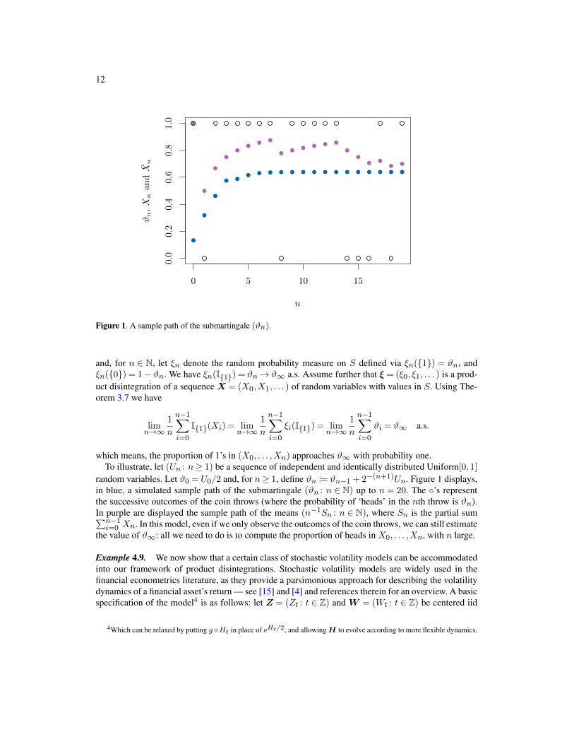
Figure 1. A sample path of the submartingale (ϑn).

and, for n ∈ N, let ξn denote the random probability measure on S defined via ξn(1) = ϑn, andξn(0) = 1− ϑn. We have ξn(I1) = ϑn→ ϑ∞ a.s. Assume further that ξ = (ξ0, ξ1, . . . ) is a prod-uct disintegration of a sequence X = (X0,X1, . . . ) of random variables with values in S. Using The-orem 3.7 we have

limn→∞

1

n

n−1∑i=0

I1(Xi) = limn→∞

1

n

n−1∑i=0

ξi(I1) = limn→∞

1

n

n−1∑i=0

ϑi = ϑ∞ a.s.

which means, the proportion of 1’s in (X0, . . . ,Xn) approaches ϑ∞ with probability one.To illustrate, let (Un : n≥ 1) be a sequence of independent and identically distributed Uniform[0,1]

random variables. Let ϑ0 = U0/2 and, for n≥ 1, define ϑn := ϑn−1 + 2−(n+1)Un. Figure 1 displays,in blue, a simulated sample path of the submartingale (ϑn : n ∈ N) up to n = 20. The ’s representthe successive outcomes of the coin throws (where the probability of ‘heads’ in the nth throw is ϑn).In purple are displayed the sample path of the means (n−1Sn : n ∈ N), where Sn is the partial sum∑n−1i=0 Xn. In this model, even if we only observe the outcomes of the coin throws, we can still estimate

the value of ϑ∞: all we need to do is to compute the proportion of heads in X0, . . . ,Xn, with n large.

Example 4.9. We now show that a certain class of stochastic volatility models can be accommodatedinto our framework of product disintegrations. Stochastic volatility models are widely used in thefinancial econometrics literature, as they provide a parsimonious approach for describing the volatilitydynamics of a financial asset’s return — see [15] and [4] and references therein for an overview. A basicspecification of the model4 is as follows: let Z = (Zt : t ∈ Z) and W = (Wt : t ∈ Z) be centered iid

4Which can be relaxed by putting g Ht in place of eHt/2, and allowingH to evolve according to more flexible dynamics.

A characterization of the strong LLN for Bernoulli sequences 13

sequences, independent from one another, and defineX andH via the stochastic difference equations

Xt = eHt/2Zt, t ∈N, and Ht = α+ βHt−1 +Wt, t≥ 1,

where α and β are real constants and whereH0 follows some prescribed distribution. The random vari-ableXt is interpreted as the return (log-price variation) on a given financial asset at date t, and theHt’sare latent (i.e, unobservable) random variables that conduct the volatility of the processX . Usually thisprocess is modelled with Gaussian innovations, that is, with Wt and Zt normally distributed for all t.In this case the random variables Xt are supported on the whole real line, so we need to consider otherdistributions for Z andW if we want to ensure that the Xt’s are compactly supported.

Our objective is to show how Theorem 3.7 can be used to estimate certain functionals of the latentvolatility process H in terms of the observed return process X . To begin with, notice that if |β| < 1and if H0 is defined via the series H0 := (1− β)−1α +

∑∞k=0 β

kW−k, then H (and X) is strictlystationary and ergodic, in which case we have that

limn→∞

1

n

n−1∑t=0

g Ht = Eg H0 (15)

almost surely, for any PH0-integrable g : SH → R, where we write SH := suppH0. Also, no-

tice that, by construction, we have for all n, all measurable A0, . . . ,An ⊆ S := suppX0 and allh= (h0, h1, . . . ) ∈ SN

H ,

P(X0 ∈A0, . . . ,Xn ∈An |H = h

)= P

(eH0/2Z0 ∈A0, . . . , e

Hn/2Zn ∈An |H = h)

(∗)= P

(eh0/2Z0 ∈A0, . . . , e

hn/2Zn ∈An |H = h)

(∗∗)= P

(eh0/2Z0 ∈A0, . . . , e

hn/2Zn ∈An)

=

n∏t=0

P(eht/2Zt ∈At

)(∗∗∗)

=

n∏t=0

P(Xt ∈At |H = h

). (16)

Where (∗) is yielded by the substitution principle, (∗∗) follows from the fact that Z and H are in-dependent (as H only depends on W ), and (∗ ∗ ∗) is just a matter of repeating the previous steps. Areasoning similar to the one used in the proof of Lemma 3.2 then tells us that P(X ∈ · |H)ω is a prod-uct measure on SN for almost all ω. Also, notice that in particular we have that P(Xt ∈A |H = h) =

P(eht/2Zt ∈ A) for all t. In fact, let ϕ : SH →M1(S) be defined via ϕ(h,A) := P(eh/2Z0 ∈ A), forh ∈ SH and measurable A⊆ S, where we write ϕ(h,A) in place of ϕ(h)(A) for convenience. Sincethe Zt’s are identically distributed, we have in particular that ϕ(h,A) = P(eh/2Zt ∈ A) for all t. Thepreceding derivations now allow us to conclude that

ϕ(Ht(ω),A) = P(Xt ∈A |Ht)ω = P(Xt ∈A |H)ω. (17)

We are now in place to introduce a product disintegration of X , by defining ξωt (A) := P(Xt ∈A |H)ω for measurable A ⊆ S, t ∈ Z and ω ∈ Ω. To see that ξ = (ξ0, ξ1, . . . ) is indeed a productdisintegration of X , first notice that ξ0(A0) · · · ξn(An) is σ(ξ)-measurable for every n and every

14

(n + 1)-tuple A0, . . . ,An of measurable subsetes of S. Moreover, defining ψ : SNH →M1(S)N via

ψ(h0, h1, . . . ) = (ϕ(h0),ϕ(h1), . . . ), we obtain, by equations (16) and (17),

E(ξ0(A0) · · · ξn(An)I[ξ∈B]

)= E

(ϕ(H0,A0) · · ·ϕ(Hn,An)I[H∈ψ−1(B)]

)= P

(X0 ∈A0, . . . ,Xn ∈An,H ∈ ψ−1(B)

)= P

(X0 ∈A0, . . . ,Xn ∈An,ξ ∈B

),

whence P(X0 ∈ A0, . . . ,Xn ∈ An |ξ) = ξ0(A0) · · · ξn(An), and then Lemma 3.2 tells us that ξ is —voilà — a product disintegration ofX .

Now, since ϕ is continuous and one-to-one, we have that ϕ is a homeomorphism from SH onto itsrange whenever SH is compact (in particular, range(ϕ) is compact, hence measurable, in M1(S)).Also, as ξt = ϕ Ht for all t, we have that Ht = ϕ−1 ξt is well defined. Suppose now that f : S→Ris a given continuous function. We have

ξωt (f) =

∫Sf(x) ξωt (dx) =

∫Sf(x)ϕ(Ht(ω),dx) =: g(Ht(ω))

and, as H is ergodic, it holds that limn→∞ n−1∑n−1t=0 ξt(f) = Eg H0, where we know that the

expectation is well defined, as E|g H0| ≤ E(∫S |f(x)| ξ0(dx)

)<∞, with the expected value given

by Eg H0 =∫S f(x)PX0

(dx). We can now apply Theorem 3.7 to see that

Eg H0 = limn→∞

n−1n−1∑t=0

f Xt.

The conclusion is that, for suitable g of the form g(h) =∫S f(x)ϕ(h,dx), we can estimate Eg H0

by the data (X0,X1, . . . ,Xn) as long as n is large enough, even if we cannot observe H . Of course,this follows from ergodicity of X , but it is interesting anyway to arrive at this result from an alternateperspective; moreover, one can use Hoeffding type inequalities as in Example 4.4 to easily derive a rateof convergence for sample means ofX based on the rate of convergence of sample means ofH .

5. Concluding remarks

In this paper we prove that a sequence of Bernoulli(p) random variables satisfies the strong law oflarge number if and only if the sequence is conditionally independent, where the conditioning is on asequence of [0,1]-valued random variables, whose corresponding sequence of sample means convergesalmost surely. As a byproduct, we introduce the concept of a product disintegration, which generalizesexchangeability. Some applications of the concept are illustrated in Section 4. Further applications ofproduct disintegrations and of Theorem 3.7 appear as a possible path to be pursued in future work.

A road not taken. At some point, during the development of the present paper, we delved into the pos-sibility of translating our approach to the language of Ergodic Theory. This proved more difficult thanwe first thought, but we did come up with a conjecture: consider the left–shift operator T acting on SN,given by (Tx)i = xi+1 for x= (x0, x1, . . . ) ∈ SN, and define T : M1 (S)N→M1 (S)N analogously.Recall that ρ(λ) :=

∏i∈N λi for λ ∈M1(S)N.

Conjecture 1. Let S be a compact metric space. A T -invariant measure q ∈M1(SN) is T–ergodic ifand only if there exists a T–ergodic measure Q ∈M1(M1 (S)N) such that q =

∫ρ (λ)Q (dλ).

A characterization of the strong LLN for Bernoulli sequences 15

Auxiliary resultsGiven a topological space S, we will write B ≤ S to mean that B belongs to the σ-field generated bythe topology of S (i.e., that B is a Borel subset S).

A.1. Spaces of measures

For a compact metric space S endowed with its Borel σ-field, let Measb(S) denote the set of measur-able, bounded maps f : S → R, let C(S) ⊆Measb(S) denote the set of continuous maps from S toR, and let M(S) denote the set of finite Borel measures on S. As in the main text, M1(S) ⊆M(S)denotes the set of Borel probability measures on S. For f ∈Measb(S), we define the evaluation mapf : M(S)→R by f(µ) :=

∫f(x)µ(dx), for µ ∈M(S).

There are a few manners through which one can introduce a σ-field on M(S) (and, a fortiori, onM1(S)). The most commonly adopted approach is to consider in M(S) the weak* topology relative toC(S) (in conventional probabilistic jargon, this is simply called the weak topology), that is, the coarsesttopology on M(S) for which, for every f ∈ C(S), its evaluation map f is continuous. The followingtheorem presents some very useful results. Item 2 is related to Prokhorov’s compactness criterion, butis not restricted to probability measures. The last three items show that, if the aim is to obtain a σ-fieldin M(S), there is no need for topological considerations (on M(S)).

Theorem A.1. Let S be a compact metric space. Then

1. M(S) is Polish (i.e. is separable and admits a complete metrization) in the weak* topology.2. A set K ⊆M(S) is weakly* relatively compact if and only if supµ∈K f(µ)<∞ for all nonneg-

ative f ∈C(S).3. The Borel σ-field relative to the weak* topology onM(S) coincides with the σ-field σ(C ), where

C can be taken as any one of the following classes:

i. C = f : f ∈C(S), f ≥ 0.ii. C = f : f = IB , B ≤ S.

iii. C = f : f ∈Measb(S).

Remark A.2. In summary, item (3) above says the following: if we write τ(f : f ∈ C(S)) for thetopology on M1(S) generated by the mappings (f : f ∈ C(S)) (that is, the weak* topology), thenσ(τ(f : f ∈C(S)

))= σ

(f : f ∈C(S)

), etc.

Proof. For the first two items, and sub-items i. and ii. of the last item, see Theorem A2.3 in [6]. Theproof will be complete once we establish the identity

σf : f ∈Measb(S)= σf : f = IB , B ≤ S.

Clearly the inclusion σf : f ∈Measb(S) ⊇ σf : f = IB , B ≤ S holds.For the converse inclusion, it is enough to show that, for every g ∈Measb(S), one has g ∈ σf : f =

IB , B ≤ S=: B. If g = IB for someB ≤ S, then clearly g ∈ B. If g is simple, with standard represen-tation g(x) =

∑nj=1 ajIAj

(x), then g(λ) =∑nj=1 aj gj(λ), where gj = IAj

. Thus, g ∈ B as it is a lin-ear combination of elements of B. For the general g ∈Measb(S), let (gn) be a sequence of simple func-tions with |gn| ≤ |g| and gn→ g. Then the Dominated Convergence Theorem gives g(λ) = lim gn(λ)and hence g ∈ B, which concludes the result.

16

Since M1(S) = µ ∈M(S) : f(µ) = 1 = f−1(1), with f = IS ∈ C(S), clearly M1(S) is aweakly* closed (hence measurable) subset of M(S). By item 2 in Theorem A.1, M1(S) is weakly*compact. Indeed, more can be said: M1(S) is a compact metrizable space. Usually, this fact is statedin terms of the so called Lévy-Prokhorov metric, which works for quite general S but suffers from a“lack of interpretability”. Conveniently, when S is compact there is an equivalent metric generatingthe weak* topology, given by d(µ,ν) =

∑k≥1 2−k

∣∣∣fk(µ)− fk(ν)∣∣∣ , where fkk≥1 is a dense and

countable subset of the unit ball in C(S). The following result is an immediate corollary to Theorem8.3.2 in [2]:

Theorem A.3. The weak* topology on M1(S) is metrizable.

A.2. Random probability measures

Definition A.4. A random probability measure on S is defined to be a Borel measurable map ξ : Ω→M1(S). We shall denote the value of a random probability measure ξ at the point ω by ξω and, for aBorel subsetB ⊆ S, we will use the notation ξω(B) and ξ(ω,B) undistinguishedly. The latter notationis justified in Theorem A.10 below.

Lemma A.5 (measurability of ξ). A map ξ : Ω→M1(S) is measurable if and only if the map ω 7→∫f dξω = f ξ(ω) is a random variable for every f ∈ C , where C can be taken as any one of the sets

C(S), Measb(S) or IB : B ≤ S.

Proof. By Theorem A.1, the Borel σ-field on M1(S) is given by

σf : f ∈C(S)= σf : f ∈Measb(S)= σf : f = IB , B ≤ S.

The ‘only if’ part follows immediately. For the ‘if’ part, notice that σf : f ∈ C is the smallest σ-field containing the sets f−1(E), with f ∈ C and E ≤R. Now f ξ is measurable for every f ∈ C iff(f ξ)−1(E) ∈F for every f ∈ C and every E ≤R iff ξ−1(G) ∈F for every G of the form f−1(E)with f ∈ C and E ≤ R. Since the class of such G generates the Borel σ-field on M1(S), the resultfollows.

Theorem A.6 (existence of Baricenter). Let (Ω,F ,P) be a probability space, S a compact metricspace, and let ξ be a random probability measure on S. Then there exists a unique element µ ∈M1(S)such that the equality

∫S f(x) µ(dx) =

∫Ω

∫S f(x) ξω(dx)P(dω) holds for all f ∈C(S).

Proof. Letϕ : C(S)→R be defined byϕ(f) :=∫

Ω

∫S f(x) ξω(dx)P(dω).Clearlyϕ(f)≥ 0 if f ≥ 0,

ϕ(αf + g) = αϕ(f) + ϕ(g), and ϕ(1) = 1. Thus, by the Riesz-Markov Theorem, there is an elementµ ∈M1(S) such that the stated equality holds.

Definition A.7. The unique element µ yielded by Theorem A.6 is called the baricenter of ξ (analo-gously: the P-expectation of ξ; analogously: the baricenter of Pξ). Notation:

µ=:

∫ξ dP =: EPξ.

We also write simply Eξ in place of EPξ when P is understood from context.

A characterization of the strong LLN for Bernoulli sequences 17

Lemma A.8. Let ξ be a random probability measure on S and let Eξ be its baricenter. Then

1. (commutativity) For each measurable subset B ⊆ S, the equality Eξ (B) = E (ξ (B)) holds;2. (maximal support) there exists a set Ω0 with P (Ω0) = 0 such that, for ω /∈ Ω0, the relation

supp ξω ⊆ suppEξ holds.

Proof. For the first item, let λ(B) := E(ξ(B)), B ⊆ S measurable. Clearly we have λ(B) ≥ 0 andλ(Ω) = 1. Moreover, if (Bj) is a sequence of measurable subsets of S which are pairwise disjointsuch that B =

⋃∞j=1Bj , then for each ω we have ξω(B) = limn→∞

∑nj=1 ξ

ω(Bj)≤ 1. Thus, by theDominated Convergence Theorem (DCT), we have λ(B) =

∑∞j=1 λ(Bj). Therefore λ is a probability

measure on S. Now let K ⊆ S be closed and let (fn) be a sequence of continuous functions on Ssuch that 1 ≥ fn(x)→ IK(x), x ∈ S. On the one hand we have Eξ(K) = limn→∞

∫fn(x)Eξ(dx),

by DCT. On the other hand, for each ω it holds that

0≤ ξω(K) = limn→∞

∫fn(x) ξω(dx)≤ ‖fn‖∞ ≤ 1,

again by DCT. Applying the DCT once more yields

λ(K) = limn→∞

∫ ∫fn(x) ξω(dx)P(dω) = lim

n→∞

∫fn(x)Eξ(dx) = Eξ(K),

where the second equality follows from the definition of the baricenter. Thus, Eξ and λ are measureson S whose values on closed sets coincide, and this implies Eξ = λ, as asserted.

For the second item, let U := S \ supp (Eξ). Then ξ (U)≥ 0 and E (ξ (U)) = Eξ (U) = 0, by item 1.Hence ξ (U) = 0 almost surely.

A.3. Probability Kernels

Definition A.9 (see [6], page 20). Given two measurable spaces (Ω,F ) and (S,S ), a map ξ : Ω×S →R is said to be a probability kernel from (Ω,F ) to (S,S ) iff

D1 For each ω ∈Ω, the map B→ ξ(ω,B) is a probability measure on S.D2 For each B ≤ S, the map ω 7→ ξ(ω,B) is F -measurable.

Kernels play an important role in probability theory, appearing in many forms, for example randommeasures, conditional distributions, Markov transition functions, and potentials [6]. Indeed, in manycircumstances, one feels more comfortable working with probability kernels instead of random prob-ability measures as defined above, given the prevalence of the former concept in the literature. Thefollowing result connects the two concepts, showing that they are indeed equivalent:

Theorem A.10. Fix two measurable spaces (Ω,F ) and (S,S ), and assume S = σ(C ) for someπ-system C . Let ξ : Ω×S → R be such that ξ(ω, ·) is a probability measure on S, for every ω ∈ Ω.Then the following conditions are equivalent:

1. ξ is a probability kernel from (Ω,F ) to (S,S ).2. ω 7→ ξ(ω, ·) is an F -measurable mapping from Ω to M1(S).3. ω 7→ ξ(ω,E) is an F -measurable mapping from Ω to [0,1] for every E ∈ C .

In particular, the above equivalences hold with C = F .

18

Proof. This is just a restatement of Lemma 1.40 in [6], by noticing that the Borel σ-field on M1(S)

coincides with σ(f : f = IB , B ≤ S) as ensured by Theorem A.1.

Definition A.11. A kernel ξ from (Ω,F0) to (S,S ) is said to be a regular conditional distributionof a random variable X : Ω→ S given a σ-field F0 ⊆F iff the equality

∫F ξ(ω,B)P(dω) = P([X ∈

B]∩ F ) holds for all B ≤ S and F ∈F0. In particular, for each B ≤ S the random variable ξ(·,B) isa version of P(X ∈B |F0).

Theorem A.12 (Regular conditional distribution — [6], Theorem 6.3). Let (S,S ) and (T,T ) bemeasurable spaces, and letX and ξ be random variables taking values in S and T respectively. Assumefurther that S is Borel. Then there exists a probability kernel η from T to S such that P(X ∈B | ξ)ω =η(ξ(ω),B) for all B ∈S and all ω in a set Ω∗ ⊆ Ω with P(Ω∗) = 1. Moreover, η is unique almosteverywhere-Pξ .

Remark A.13. In the conditions of the above Theorem, one can introduce a probability kernel η′ from(Ω, σ(ξ)) to (S,S ) by putting η′(ω,B) := η(ξ(ω),B). Also, if ξ is the identity map and (T,T ) =(Ω,F0), where F0 ≤F , then automatically η is a kernel from Ω to S which is a regular version ofP(X ∈ · |F0).

A.4. Product spaces

Lemma A.14 (Product and Borel σ-fields — [6], Lemma 1.2). Let S have topology τ and let S :=σ (τ) be the Borel σ-field on S. Let τN be the product topology on SN and let S N be the product(cylindrical) σ–field on SN. If S is metrizable and separable, then σ(τN) = S N, that is, S N is theBorel σ-field on SN.

Corollary A.15. Let S be a separable metric space with topology τ , and let B be a countable basisfor τ which is stable under finite intersections. For each n ∈N and each B0, . . . ,Bn ∈B, define

C (n;B0, . . . ,Bn) :=B0 × · · · ×Bn × S × · · · ⊆ SN. (18)

Let C denote the collection of all sets of the form (18). Then C is a countable π-system which generatesthe Borel σ-field on SN.

Remark A.16. The set B above can be obtained as follows: let D be a countable, dense subset ofS, and let D be the collection of all balls with centers in D and rational radii. Now let Bn, n ≥1, be the collection formed by all intersections of n elements of D , that is, B ∈Bn iff there existx1, . . . , xn ∈D and r1, . . . , rn ∈ Q such that B =

⋂ni=1 ball(xi; ri). Clearly, each Bn is countable.

Now let B :=⋃n≥1 Bn.

Proof of Corollary A.15. We begin by proving that C is indeed a π-system. Clearly, C is non-empty.Now, let A0, . . . ,Am,B0, . . . ,Bn ∈B and consider C (m;A0, . . . ,Am),C (n;B0, . . . ,Bn). Withoutloss of generality, suppose n≥m. Then

C (m;A0, . . . ,Am)∩C (n;B0, . . . ,Bn) =A0 ∩B0 × · · · ×Am ∩Bm × · · · ×Bn × S × . . .

= C (n;A0 ∩B0, . . . ,Am ∩Bm, . . . ,Bn).

A characterization of the strong LLN for Bernoulli sequences 19

Since B is stable under finite intersections, Ai ∩ Bi ∈ B, for each i ∈ 0, . . . ,m, and the resultfollows.

It remains to show that C generates the Borel σ-field on SN. Clearly any A ∈ C is a Borel set inSN. For the reverse inclusion, by Lemma A.14 and the facts that σ(τ) = σ(B) and σ(τN) = σ(BN), itsuffices to prove that given Ai+∞i=0 a sequence of elements in B, it holds thatA=A0 ×A1 × · · · ×An ×An+1 × · · · ∈ σ(C). For each m ∈ N, define A(m) = A0 × · · · ×Am × S × . . . , i.e., A(m) =

C (m;A0, . . . ,Am). Surely, for each m ∈ N, A(m) ∈ σ(C). Furthermore, note that A= ∩+∞m=0A

(m),so that A ∈ σ(C).

A.5. Additional auxiliary results

Definition A.17. Two measurable spaces (M,M ) and (N,N ) are said to be Borel isomophic if thereexists a bijection h : M →N such that both h and h−1 are measurable. A measurable space (M,M )is said to be a Borel space if it is Borel isomorphic to a Borel subset of the interval [0,1].

Definition A.18. A topological space M is said to be a Polish space iff it is separable and admits acomplete metrization.

Theorem A.19 ([6], Theorem A1.2). Let M be a Polish space. Then every Borel subset of M is aBorel space.

Lemma A.20 (Doob-Dynkin Lemma — [6], Lemma 1.13). Let (M,M ) and (N,N ) be measurablespaces, and let f : Ω→M and g : Ω→N be any two given functions. If M is Borel, then f is σ(g)-measurable if and only if there exists a measurable mapping h : N →M such that f = h g,

Theorem A.21 (Riesz-Markov). Let S be a locally compact Hausdorff space and ϕ a positive linearfunctional on Cc(S). Then there is a unique Radon measure µ on the Borel σ-field of S for whichϕ(f) =

∫S f(x)µ(dx) for all f ∈ Cc(S). In particular, if S is compact and ϕ(1) = 1, then µ is a

probability measure.

Theorem A.22 (Kolmogorov’s strong law of large numbers). LetX := (X0,X1, . . . ) be an indepen-dent sequence of random variables such that supnVar (Xn)<∞. Then it holds that

limn→∞

n−1n−1∑i=0

(Xi −EXi) = 0

almost surely.

Theorem A.23 (range and inverse, Kuratowski — [6], Theorem A1.3). Let f be a measurable bijec-tion between two Borel spaces S and T . Then the inverse f−1 is again measurable.

Acknowledgements

The author Luísa Borsato is supported by grant 2018/21067-0, São Paulo Research Foundation(FAPESP).

The author Eduardo Horta wishes to thank MCTIC/CNPq (process number 438642/2018-0) for fi-nancial support.

20

References

[1] Bernoulli, J. (2005). On the law of large numbers. [Translation by O.B. Sheynin into English of thePars Quarta of Ars Conjectandi.] Available at www.sheynin.de/download/bernoulli.pdf

[2] Bogachev, V. (2007) Measure Theory, Springer-Verlag, Berlin. doi:10.1007/978-3-540-34514-5.

[3] Cardano, G. (2015) The book on games of Chance: the 16th-century treatise on probability. CourierDover Publications.

[4] Davis, R. and Mikosch, T. (2009) Probabilistic Properties of Stochastic Volatility Models. In T.Mikosch, J.P. Kreiß, R. A. Davis and T. G. Andersen (eds.), Handbook of Financial Time Series(pp. 255–267). Berlin/Heidelberg: Springer. doi:10.1007/978-3-540-71297-8_11.

[5] Horta, E. and Ziegelmann, F. (2018) Conjugate processes: Theory and application to risk fore-casting, Stochastic Processes and their Applications 128 (3) 727–755. doi:10.1016/j.spa.2017.06.002.

[6] Kallenberg, O. (2002) Foundations of Modern Probability, Probability and its Applications,Springer-Verlag, New York. doi:10.1007/b98838.

[7] Kuczmaszewska, A. (2011) On the strong law of large numbers for ϕ-mixing and ρ-mixing random variables, Acta Mathematica Hungarica 138 174–189. doi:10.1007/s10474-011-0089-z.

[8] Kontorovich, A. and Brockwell, A. (2014) A Strong Law of Large Numbers for Strongly MixingProcesses, Communications in Statistics - Theory and Methods 43 (18) 3777–3796. doi:10.1080/03610926.2012.701696.

[9] Loève, M. (1973). Paul Lévy, 1886-1971. The Annals of Probability, 1 (1) 1–8. doi:10.1214/aop/1176997021.

[10] Petersen, A. and Müller, H-G. (2016). Functional data analysis for density functions by transfor-mation to a Hilbert space. Annals of Statistics, 44 (1) 183–218. doi:10.1214/15-AOS1363.

[11] Poisson, S.D. (1837). Recherches sur la probabilité des jugemens en matière criminelle at enmatière civile, précédés des règles générales du calcul des probabilités. Paris: Bachelier.

[12] Popper, K. (1959) The propensity interpretation of Probability. The British Journal for the Phi-losophy of Science 10 (37) 25–42.

[13] Seneta, E. (1992) On the history of the Strong Law of Large Numbers and Boole’s inequality.Historia Mathematica 19 (1) 24–39. doi:10.1016/0315-0860(92)90053-E.

[14] Seneta, E. (2013) A Tricentenary history of the law of large numbers. Bernoulli 19 (4) 1088–1121.doi:10.3150/12-BEJSP12.

[15] Shephard, N. and Andersen, T. G. (2009) Stochastic Volatility: Origins and Overview. In T.Mikosch, J.P. Kreiß, R. A. Davis and T. G. Andersen (eds.), Handbook of Financial Time Series(pp. 233–254). Berlin/Heidelberg: Springer. doi:10.1007/978-3-540-71297-8_10.

[16] Taylor, R. L. and Hu, T-C. (2018) On laws of large numbers for exchangeable random variables,Stochastic Analysis and Applications 5 (3) 323–334. doi:10.1080/07362998708809120.

[17] Hu, T.C., Rosalsky, A. and Volodin, A. (2008) On convergence properties of sums of dependentrandom variables under second moment and covariance restrictions, Statistics and Probability Let-ters 78 1999–2006. doi:10.1016/j.spl.2008.01.073.