This paper can be downloaded without charge at:

The Fondazione Eni Enrico Mattei Note di Lavoro Series Index: http://www.feem.it/Feem/Pub/Publications/WPapers/default.htm

Social Science Research Network Electronic Paper Collection:

http://ssrn.com/abstract=960725

The opinions expressed in this paper do not necessarily reflect the position of Fondazione Eni Enrico Mattei

Corso Magenta, 63, 20123 Milano (I), web site: www.feem.it, e-mail: working.papers@feem.it

A CGE-Analysis of Energy Policies Considering Labor Market

Imperfections and Technology Specifications

Robert Küster, Ingo Ellersdorfer and Ulrich Fahl

NOTA DI LAVORO 7.2007

JANUARY 2007 CCMP – Climate Change Modelling and Policy

Robert Küster, Ingo Ellersdorfer and Ulrich Fahl, Institute of Energy Economics and the

Rational Use of Energy, Department Energy Economics and System Analyses Universität Stuttgart

A CGE-Analysis of Energy Policies Considering Labor Market Imperfections and Technology Specifications Summary The paper establishes a CGE/MPSGE model for evaluating energy policy measures with emphasis on their employment impacts. It specifies a dual labor market with respect to qualification, two different mechanisms for skill specific unemployment, and a technology detailed description of electricity generation. Non clearing of the dual labor market is modeled via minimum wage constraints and via wage curves. The model is exemplarily applied for the analysis of capital subsidies on the application of technologies using renewable energy sources. Quantitative results highlight that subsidies on these technologies do not automatically lead to a significant reduction in emissions. Moreover, if emission reductions are achieved these might actually partly result from negative growth effects induced by the promotion of cost inefficient technologies. Inefficiencies in the energy system increase unemployment for both skilled and unskilled labor.

Keywords: CGE, Energy Economic Analysis, Employment Impact, Choice of Technology JEL Classification: Q42, Q43, Q48, Q52

This paper was presented at the EAERE-FEEM-VIU Summer School on "Computable General Equilibrium Modeling in Environmental and Resource Economics", held in Venice from June 25th to July 1st, 2006 and supported by the Marie Curie Series of Conferences "European Summer School in Resource and Environmental Economics".

Address for correspondence: Robert Küster Universität Stuttgart Heßbrühlstr. 49a 70565 Stuttgart Germany Phone: +49 0711 685 87831 Fax: +49 0711 685 87873 E-mail: rk@ier.uni.stuttgart.de

1. Introduction The relationship between environmental policy and employment has been theoretically discussed since the 1970s and numerically assessed subsequently.1 Environmental outcome is strongly affected by the design of energy systems. Currently, decisions on energy systems are determined by climate policy endeavors, market liberalization, and the strong necessity for replacement and extension of generation capacities in the national power plant system. Amidst persistently high unemployment rates in Europe, upcoming decisions on future energy systems create a current need for research on the employment impacts of alternative environmental and energy policies. CGE modeling provides an established instrument for the quantification of the impacts of energy and environmental policy measures on the economy. The neoclassical principles of any CGE model imply flexible prices and market clearing for labor just as for any other good or factor of production. Consequently, standard CGE models do not take into account the non-clearing of the labor market as it occurs in reality and as it is of high importance for any economic assessment. The resulting research implication is the modeling of involuntary equilibrium unemployment. With respect to energy economics, it has been discussed mainly in the context of the double dividend hypothesis by e.g. Böhringer et al. (2001), Koschel (2001), Böhringer et al. (1997), and Carraro et al. (1996). Labor demand and unemployment differ between qualification, i.e. skill type of labor. For instance, as Reinberg and Hummel (2003) show for Germany throughout the last two decades the unemployment rate amongst unskilled labor was about three times higher than it was for skilled. Disaggregating labor input by skill level has recently been introduced to energy policy assessments, as e.g. in Faehn et al. (2004), Niez and Sue Wing (2004), Bosello and Carraro (2001), and Hill (1998). Most energy policy instruments are technology oriented. The choice of technologies determines the economic and ecological outcome induced by a policy measure. As Fahl et al. (2005) point out this includes the energy system’s employment impact. Consequently, a CGE analysis of the economic implications of alternative energy systems needs to explicitly incorporate both the labor market behavior as well as energy technology specifications. Chapter 2 formulates a CGE model that aims at meeting these requirements. It includes a dual labor market which allows not only for considering skill specific unemployment rates. As chapter 3 discusses a dual labor market also permits a distinct modeling of different causes for unemployment that each skill type is subject to. Here, involuntary unemployment of skilled workers is related to a wage curve. Unskilled labor’s unemployment is due to a minimum wage formulation, i.e. downward rigid wages. In Chapter 4 the model is exemplarily applied for the assessment of CO2 allowance trade and

1 For a recent overview see OECD (2004).

1

subsidies on renewable energy sources (RES). Chapter 5 concludes and identifies research implications.

2. Model description

2.1 Composition and aggregation level The model applied in this paper is a multi regional, multi sectoral Arrow-Debreu general equilibrium model. It is formulated as a system of non-linear equations in the programming language GAMS/MPSGE by Brooke et al. (1996) and Rutherford (1987). The model itself is based on GTAP-EG by Rutherford and Paltsev (2000) and on Böhringer (1996). It has been further developed and applied by e.g. Küster et al. (2006) and Zürn et al. (2005). Underlying data for production and trade follows the economic input-output concept and is consistently provided by the GTAP6 database (cf. GTAP 2005). The model accounts for ten regions. Regional aggregation is indicated in table 1. In each region 13 industries as shown in table 2, of which five are energy sectors, produce output by applying four primary factors, given in table 3. Primary factors are capital, skilled labor, unskilled labor, and exhaustible energy resources. Natural resources other than primary energy carriers are not accounted for. In GATP6 these are forest and fish stock, which here are mapped to capital. Primary factors are regionally immobile but mobile between sectors. Households and government are represented by a single regional representative agent. Table 1: Regional composition2

Region Definition Countries within region (GTAP acronym)

1 DEU Germany DEU

2 OEU Old EU15 w/out Germany

AUT, BEL, DNK, FIN, FRA, GBR, GRC, IRL, ITA, LUX, NLD, PRT, ESP, SWE

3 NEU New EU members CYP, CZE, HUN, MLT, POL, SVK, SVN, EST, LVA, LTU

4 EAB All other European Annex B countries ROM, BGR, CHE, XEF, HRV(*)

5 RUS Annex-B country Russia RUS

6 RAB Rest of Annex-B CAN, JPN, NZL

7 REJ Annex B Rejecting Countries USA, AUS

8 OPE OPEC countries IDN, VEN, XNF, XME

9 CHI China and India CHI, HKG, IND

10 ROW Rest of World All other 43 GTAP regions (**),(***)

2 (*) Croatia (HRV) has not ratified Kyoto yet but it is assumed that in the course of EU accession ratification will soon be carried out. (**) Rest of Sub-Saharan Africa (XSS) contains the OPEC country Nigeria. However, because there are numerous other countries incorporated in XSS, this group is mapped to ROW. (***) Ukraine is part of Rest of former Soviet Union (XSU). Data for the single country Ukraine is not available in GTAP6. Hence, this Annex-B country cannot be accounted for as climate protection ally.

2

Table 2: Sectoral composition

Energy sectors Non-energy sectors Coal COL Chemical, rubber, plastic products CHM

Natural gas GAS Machinery and equipment MAC

Crude oil CRU Buildings BUIL

Petroleum OIL Transport TRN

Electricity ELE Agriculture and forestry AGR

Paper products, publishing PPP

Iron and steel I_S

Rest of the economy, incl. services Y

Table 3: Primary input factors

Primary input factors Skilled labor SKL Unskilled labor USK Capital (including land) K Exhaustible energy resources R

Following Arrow and Debreu (1954), markets are assumed to be perfectly competitive so that for all economies equilibria are induced via flexible prices. As shown by Mathiesen (1985) the economic equilibrium can be determined by a system of nonlinear equations as a mixed complementarity problem. Three corresponding equilibrium conditions must be satisfied, namely (a) zero profit condition, (b) cleared market condition, and (c) income balance condition. The zero profit condition requires that any economic activity carried out must earn zero profit. Hence, firms maximize their profits subject to their production function by minimizing costs. The cleared market condition requires that any good produced by a firm has a positive price that balances supply and demand. Goods in excess supply have a zero price. The income balance condition means that goods are acquired by agents under an income constriction. An equilibrium is characterized by a set of quantities and prices for all goods and all factors that fulfill these three conditions.

2.2 The basic model

2.2.1 The static model

Any applied general equilibrium model is characterized by a comprehensive perception of the circular flow economy. Figure 1 illustrates the major economic activities modeled. Production is modeled by nested, linear homogeneous CES production functions which relate production factors according to elasticities of substitution. Primary production factors are capital including land, exhaustible natural resources and labor. Following Arrow et. al (1961) production Y in a single economy r is realized by inputs of capital K, labor L, the intermediate product energy E, and non-energy intermediates i.e. material M (KLEM structure).

3

Investments

Foreign trade

Tax revenue

Implicit tax system

Factor markets

Savings

Carbon

Capital

Resources

Labor

Aggregationpool

(Armington)

Sectoralproduction

Internat. transport

Households and government

Utility

Production

Consumption

Representative agent

Fossil fuel production

Imports

Exports

Investments

Foreign trade

Tax revenue

Implicit tax system

Factor markets

Savings

Carbon

Capital

Resources

Labor

Carbon

Capital

Resources

Labor

Aggregationpool

(Armington)

Sectoralproduction

Internat. transport

Households and government

Utility

Production

Consumption

Representative agent

Fossil fuel production

Imports

Exports

Figure 1: Model overview circular flow structure

For a simplified general model description one may abstract from specific nesting structures to show that an economy’s output is given by

(1) ( ) YYYYYr

Mrr

Err

Lrr

Krrrrrr MELKMELKfY ρρρρρ θθθθ

1

)(,,, ⋅+⋅+⋅+⋅==

Production factor inputs are weighted by a particular share parameter θ. The sum of share parameters equates to unity which reflects constant returns to scale. Factors are related to one another by constant factor substitution elasticities of σ = 1/(1 - ρY) where (-∞<ρ<1). As indicated in figure 1 output may be exported or enter an Armington aggregate. As opposed to a Heckscher-Ohlin economy, Armington (1996) considers imported and domestic products to be imperfect substitutes. Hence, the Armington aggregate Ar composes of imports IMr and of not exported domestic intermediate production (Yr - EXr). Imports and domestic absorption are linked to each other by an Armington elasticity parameter ρA.

(2) ( ) ( )[ ] AAA

rIMrr

EXrr

Yrrrrr IMEXYIMEXYfA ρρρ

θθθ1

,, +−==

International trade flows EXr and IMr are connected to a production function that reflects international transport services. Produced Armington goods may either be redirected as intermediates into the production process or consumed by the representative agent. Domestic consumption results as (3) )( rr AfC = .

Utility is only generated through consumption. Investment is exogenously given by a savings investment identity and a corresponding fixed savings rate. Investment does not enter the

4

utility function. Leisure is not considered. Hence, utility of the representative agent in region r is given by

(4) )( rr CfU = .

The basic model is closed by limiting consumption through an income restriction for the representative household. Income Π is generated on the perfectly competitive factor markets by selling endowments of production factors labor L, capital K, and exhaustible resources R, with their respective equilibrium prices w, r, and π.

(5) rrrrrrrrrrr ZITRKrLw ζπΠ +−+++=

Primary and intermediate factor inputs as well as output of any economic activity may be taxed. Factor taxes and commodity taxes are modeled as given in GTAP-EG (cf. Rutherford and Paltsev 2000). Aggregate tax income T accrues to the representative agent and increases the budget. As part of the income is used for investment, budget to be allocated for consumption purposes is reduced by investment I. If emission trading schemes are included, CO2 allowances Z priced by ζ become part of the factor endowment.

2.2.2 Model dynamics

Dynamics can in principle be incorporated by two different means which differ in the way that economic agents handle decision problems. In an intertemporal dynamic CGE model economic agents have perfect foresight and rational expectations with respect to the entire time horizon. Their behavior is subject to an intertemporal optimization problem. Consequently, intertemporal substitution possibilities are accounted for. In a recursive dynamic CGE model agents are myopic. There is no intertemporal dimension of decision variables. Decision making is static and a sequence of static equilibria is solved. Equilibria are connected with one another by augmentation of primary factor endowments. Capital investment may either be exogenous or endogenous. Exogenous investment is determined by a given savings rate and a savings investment identity. In the endogenous case investment decisions are based upon return to capital and cost of capital (cf. Springer 1999). For this paper, the model is solved recursive dynamically with exogenously determined investments. Equilibria are solved in five year steps starting with the benchmark year 2001 up to 2030. Dynamics are based upon the neoclassical Solow-Swan model. However, instead of a balanced growth path, growth rates for factor variables differ. This is done in order to calibrate economic development to projected growth as provided by the models POLES (cf. European Commission 2003) and PRIMES (cf. European Commission 2004). There is no explicit investment function. In its place neoclassical theory states that on a competitive capital market the price of capital equilibrates savings and investments. Investment I in period t equals savings s in period t and savings are given through a constraint that sets the savings rate constant. Taking into account depreciation of capital, this leads to a regional capital stock formation of (6) ( ) 1,,1, 1 ++ +−= trtrtr IKstKst δ .

5

Investments I undertaken in the current period t augment the capital stock Kst in period t+1. As in the GTAP database, the depreciation rate δ is assumed to be constant at 4 % for any region. Equation (6) describes the augmentation of a capital stock through investments. However, input-output (I-O) data does not account for capital stock but for capital earnings, which are considered capital input. For a CGE model built upon I-O data the same holds true. If investments were to raise capital earnings in full scope, then capital input into the I-O system and hence into production would grow excessively. Consequently, growth in capital stock needs to be translated into growth in capital earnings. In the model at hand, this stock to flow conversion is done by computing the share of capital earnings to capital stock in the benchmark and using this share for scaling investments in equation (6). Then, with capital earnings determined by the return to capital r capital endowment K is given by (7)

( ) t,rt,r

t,rt,rt,r1t,r I

KstKr

Kstδ1K +=+ .

The formulation of capital augmentation is strongly dependent on capital mobility. Here, all capital is modeled regionally immobile because the stock represents physical capital. In a more complex model, capital may be described as imperfectly mobile. In such a putty-clay model one can take into account that investment decisions are in fact regionally mobile but installed capital is vintage and hence immobile. This would better describe investment decision under prevailing actual capital markets, as pointed out by Springer (2002). Fossil fuel resource endowment in region r is assumed constant over time and given by (8) ortrtr RRR ,,1, ==+ .

Regional labor supply growth is exogenous at rate g. This growth parameter incorporates population changes, human capital formation, and increases in labor productivity. (9) ( ) trLtr LgL

tr ,1, ,1+=+

In addition to the stylized aggregate economy description, any multi-sector CGE model requires that each industry i is modeled by a specific nested CES production function. All industry production functions as a whole replace the aggregate output of equation (1). Before representing particular production functions in detail, their input factor labor is specified by skill type.

2.3 Modeling heterogeneous labor The differentiation of labor by qualification can in principle be performed following a variety of categories and up to various details or levels of qualification. For instance, in a single country CGE model Lofgren (2001) distinguishes between four types of skill categories determined by educational level. The paper at hand provides a dual differentiation between highly qualified (skilled) and less qualified (unskilled) labor input. It follows Liu et al. (1998) and applies the International Standard Classification of Occupations (ISCO-88) of the International Labor Organization (ILO) (cf. ILO 2006a). Consequently, differentiation is

6

based upon occupational categories rather than education levels but as Liu et al. (1998) point out occupation and education tend to correlate with each other. Also, data availability is superior for occupational differentiation as the relevant input-output data is provided by GTAP6. In the basic model of chapter 2.2 disaggregating labor L by qualification implies to substitute homogenous supply L through skilled labor supply SKL and unskilled labor supply USK. The equilibrium price wr is replaced by skill specific equilibrium wages. For the labor dynamics, in principle the skill and unskilled decomposition requires a differentiation into skill specific labor supply augmentation. However, due to data restrictions the model at hand applies identical growth parameters for skilled labor supply SKL and unskilled labor supply USK. Regarding the sector specific production functions, heterogeneous labor inputs necessitate a modification of the usual nesting structures. Nesting structures are decisive for the effect of relative price changes induced through e.g. energy system decisions. With regards to dual labor the definition of nested CES function is essentially a question of skill differentiated substitution possibilities as discussed in e.g. Ochsen and Welsch (2004). For CGE modeling, three major alternative implementations can be identified. The Single Primary Factor Nest approach assumes that all four primary input factors can be introduced on a single nesting level under one prevailing substitution elasticity. This implies that all factors are direct substitutes. Applications can be find e.g. in Greenaway et al. (2002), and in Rutherford and Paltsev (2000). The Direct Labor Substitutability approach suspends the direct composition assumption. Instead it aggregates skilled and unskilled labor on a distinctive nesting level. Value added is generated on a higher nesting level, where the thus created labor aggregate combines with capital and resource input. Consequently, substitution relations between the two types of labor can be taken into account discretely. This concept has been carried out e.g. by Niez and Sue Wing (2004), and Faehn et al. (2004). On the other side, the Capital-Skill Complementarity theory, as developed by Griliches (1969), suggests that capital and skilled labor are complementary. Thus, they need to be modeled by a low elasticity of substitution or even by a Leontief nesting. On a higher nesting level, this capital-skill composition is integrated with other production factors. The capital-skill complementarity is applied e.g. in Böhringer et al. (2005). The different nesting possibilities allow for taking into account inter industry differences in substitution possibilities and production structures. This is realized by differentiating the nesting structures according to the industry specific factor intensities. Following the GTAP6 data the factor intensities of the 13 sectors aggregated over all regions modeled is shown in figure 2.

7

0%

10%

20%

30%

40%

50%

60%

70%

80%

90%

100%

1 C

OL

2 G

AS

3 C

RU

4 O

IL

5 E

LE

6 A

GR

7 C

HM

8 M

AC

9 B

UIL

10 T

RN

11 P

PP

12 I_

S

13 Y

Resources

Unskilled Labor

Skilled Labor

Capital

Figure 2: Sectoral primary factor intensities following GTAP6, average over all regions

The assumption is that in general industries can be described according to the concept denominated single primary factor nest. The exception is capital intensive industries which are characterized by direct labor substitutability and a value added nest that allows only modest substitution between the labor aggregate and capital. The idea is to stress the importance of capital in capital intense production. With the sectoral disaggregation applied here, these industries are the conversion industries, namely refinery and electricity production.3 The idea behind this assumption is that in the conversion sector large part of the capital used is indispensable. Thus a rather limitational elasticity between labor and capital aims at avoiding unrealistic substitution patterns.4 In addition, the electricity sector as part of the conversion sector is treated in a more complex technology detailed way (see chapter 2.4). The categorization of nesting structures yields four types of production functions as summarized in table 4. Table 4: Categorization of nesting structures Sectors Nesting concept 1 CHM, MAC, BUIL, TRN, AGR, PPP, I_S, Y Single primary factor nest + other nests 2 COL, CRU, GAS Single primary factor nest + exhaustible resources 3 OIL Direct labor substitutability + other nests 4 ELE Technology detailed

The first category includes all non energy sectors. Labor inputs are modeled in the style of the single primary factor nesting concept. Capital K, skilled labor SKL, and unskilled labor USK are linked through a Cobb Douglas function in the valued added nest with their respective

3 The threshold for capital intensity is set at a capital share of 60 % in primary input. 4 The principle possibility of unrealistic substitutions is also mentioned in Smajgl (2001).

8

shares θK, θSKL, θUSK and =1. The substitution elasticity σ is given via the parameter ρ as σ = 1/(1 - ρ), with (-∞<ρ<1). Value added is combined on the next level with the energy aggregate. The energy aggregate itself is a composite of electricity, coal, gas, oil and if applicable CO

USKSKLK θ+θ+θ

2 allowances. The final KLEM aggregate is formed on the upper level by a Leontief function, i.e. σKLEM=0 (ρKLEM=-∞). Here, the production function for all sectors other than conversion or exhaustible resource production can be formulated as in equation (10). Figure 3 illustrates the corresponding nesting structure.5

(10)

( )( )oil,ele,xei

;

USKSKLKE

M

Y

KLEMi

KLEi

KLEMi

KLEiUSK

iSKLi

Ki

KLEi

KLEMi

iUSKii

SKLii

Ki

Eii

Ei

j

Mi,ji,j

j

Mi,j

i

∉

⎥⎥⎥⎥⎥

⎦

⎤

⎢⎢⎢⎢⎢

⎣

⎡

⎥⎦⎤

⎢⎣⎡ θ+θ+θθ−+θ

⎟⎟⎠

⎞⎜⎜⎝

⎛θ−+⎟⎟

⎠

⎞⎜⎜⎝

⎛θ

=

ρ

ρ

ρρδδδρ

ρ ∑∑1

1

1

σKLEM

σKL σE

σKLE

σFE

σCOL

σLIQ

σGAS σOIL

Material

SkilledElectricity

CO2 Gas Coal Oil CO2 CO2

Unskilled

Output

Capital

Figure 3: Nesting structure for all non-energy sectors

For the production of exhaustible energy resources in the sectors crude oil, gas, and coal production (xe) the elasticity between energy resources R and value added depends on the value share of resource inputs, following Rutherford and Paltsev (2000). Further inputs within the KLEM nest are linked as a Leontief composite because the sectors are considered as fixed technology descriptions. The production function with ρ as σKLEM=0 (ρKLEM=-∞) and the nesting structure result as in equation (11) and in figure 4 respectively.

5 For simplicity production functions are not defined over r in this representation.

9

(11) ( )

xei

;MUSKSKLK

R

Y

Si

KLEMi

Si

KLEMi

KLEMi

KLEMi

KLEMi

Si

ji,j

Mi,ji

USKii

SKLii

Ki

Rii

Ri

i

∈

⎥⎥⎥⎥

⎦

⎤

⎢⎢⎢⎢

⎣

⎡

⎥⎥⎦

⎤

⎢⎢⎣

⎡⎟⎟⎠

⎞⎜⎜⎝

⎛θ+θ+θ+θ

θ−+θ

=

ρ

ρ

ρ

ρρρρ

ρ

∑

1

1

σS

σKLEM

Primary energy carrier

Capital Skilled Material Energy Unskilled

Energy resource output

Figure 4: Nesting structure of production function for exhaustible resource production

For the capital intensive oil sector the concept of the direct labor substitutability yields a production function as in equation (12). (12) ( )

( )

( )

( )

( )[ ]oili

;

USKSKL

K

E

M

Y

KLEMi

KLEi

KLEMi

KLi

KLEi

Li

KLi

Li

Li

KLi

KLEi

KLEMi

iSKLii

SKLi

Kii

Ki

Ei

Ei

jM

i,j

i,jjM

i,j

i

∈

⎥⎥⎥⎥⎥⎥⎥⎥⎥⎥

⎦

⎤

⎢⎢⎢⎢⎢⎢⎢⎢⎢⎢

⎣

⎡

⎥⎥⎥⎥⎥⎥⎥

⎦

⎤

⎢⎢⎢⎢⎢⎢⎢

⎣

⎡

⎥⎥⎥⎥⎥

⎦

⎤

⎢⎢⎢⎢⎢

⎣

⎡

⎥⎥⎦

⎤

⎢⎢⎣

⎡θ−+θ

θ−+θ

θ−+θ

θ−+

θ

=

ρ

ρ

ρ

ρ

ρ

ρ

ρρρ

ρ

ρ

ρ

∑

∑1

1

1

1

1

Factor specific value shares of produced output are given by θ. Skilled labor SKL and unskilled labor USK form a nest with a relative low elasticity of substitution. The labor aggregate is combined with capital K to generate the value added on the KL-nest. On the next level, the energy aggregate is added. The upper level combines the resulting KLE-nest with non energy intermediate inputs to a KLEM aggregate. The corresponding nesting structure for the oil sector is displayed in figure 5.

10

σKLEM

σKLσE

σKLE

σFE

σCOL

σLIQ

σGAS σOIL

Material

Capital

SkilledElectricity

CO2 Oil Gas Coal CO2 CO2

Unskilled

σL

Refined petroleum output

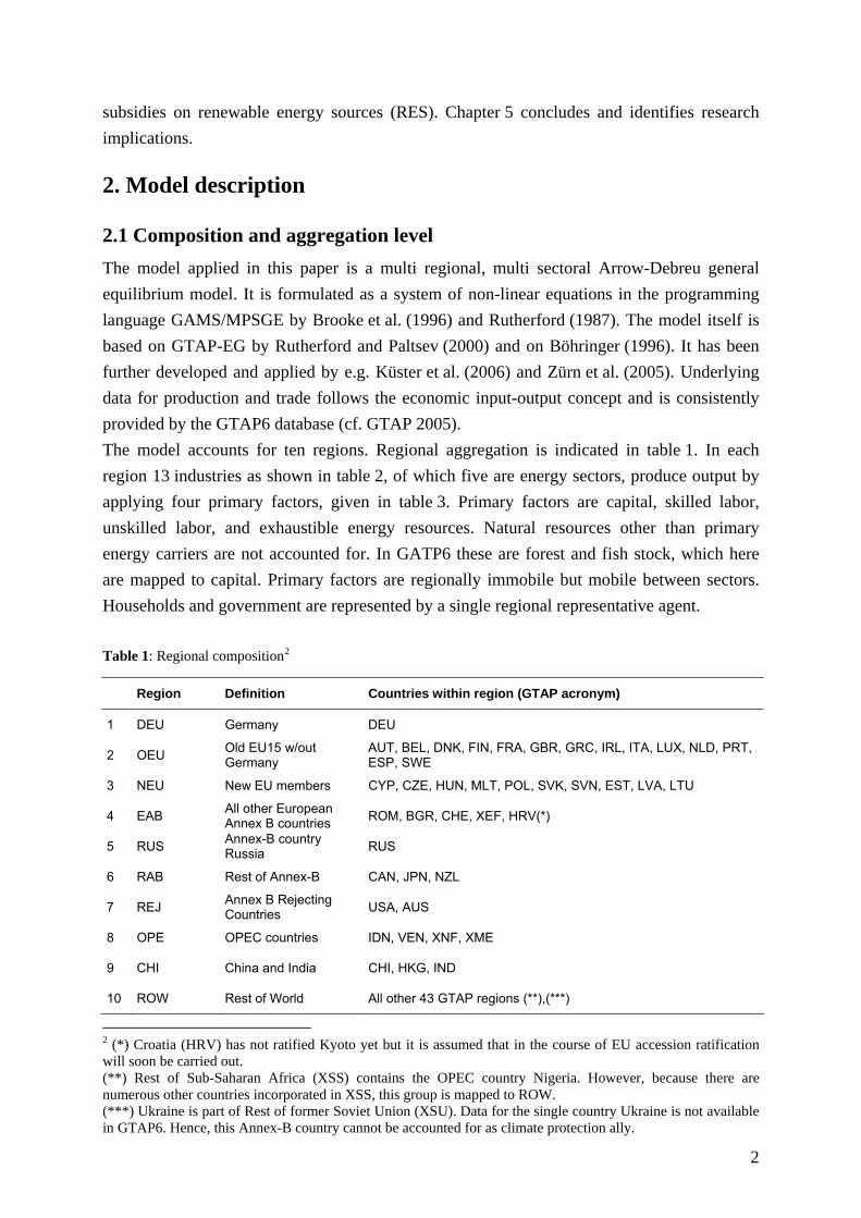
Figure 5: Nesting structure for refined petroleum production

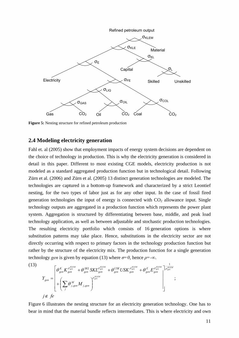
2.4 Modeling electricity generation Fahl et. al (2005) show that employment impacts of energy system decisions are dependent on the choice of technology in production. This is why the electricity generation is considered in detail in this paper. Different to most existing CGE models, electricity production is not modeled as a standard aggregated production function but in technological detail. Following Zürn et al. (2006) and Zürn et al. (2005) 13 distinct generation technologies are modeled. The technologies are captured in a bottom-up framework and characterized by a strict Leontief nesting, for the two types of labor just as for any other input. In the case of fossil fired generation technologies the input of energy is connected with CO2 allowance input. Single technology outputs are aggregated in a production function which represents the power plant system. Aggregation is structured by differentiating between base, middle, and peak load technology application, as well as between adjustable and stochastic production technologies. The resulting electricity portfolio which consists of 16 generation options is where substitution patterns may take place. Hence, substitutions in the electricity sector are not directly occurring with respect to primary factors in the technology production function but rather by the structure of the electricity mix. The production function for a single generation technology gen is given by equation (13) where σ=0, hence ρ=-∞. (13)

fej

M

EUSKSKLK

Y

KLEMgen

KLEMgen

KLEMgen

KLEMgen

KLEMgen

KLEMgen

jgenj

Mgenj

genEgengen

USKgengen

SKLgengen

Kgen

gen

∉

⎥⎥⎥⎥

⎦

⎤

⎢⎢⎢⎢

⎣

⎡

⎟⎟⎠

⎞⎜⎜⎝

⎛+

+++

=∑

;

1

,,

ρ

ρ

ρρρρ

θ

θθθθ

Figure 6 illustrates the nesting structure for an electricity generation technology. One has to bear in mind that the material bundle reflects intermediates. This is where electricity and own

11

consumption as part of the generation technology inputs are accounted for. Moreover, there is no multifuel option. Each fossil fired generation technology relies on a single energy input, which is why there is no need to further separate the energy composite.

Electricity technology output

Material CO2

σKLEM:0

UnskilledSkilled Capital Energy Figure 6: Nesting of Leontief production function for generation technologies

The electricity sector as a whole is displayed in figure 7. Specific elasticities of substitutions are implemented in every nest and reflect different ease of substitution on inter- and intraload levels and for fluctuating and constant generation levels. Total

electrici-ty

output

Fluctu-ating

energy sources

Base and

middle load

Peak load

Wind

Solar

Base load

Middle

load

Lignite

Nuclear

Hydro

Biomass

Geo-

thermal

Hard coal

Gas CC

Oil

Gas CC

Hard Coal

Oil

Hydro

pumped

Oil und

Gas

Gas GT

Oil GT

Figure 7: Nesting structure of the electricity sector6

The detailed bottom-up description of the electricity production sector requires that aggregate economic data of the GTAP6 database is expanded, as e.g. pointed out by Sue Wing (2004). Following Zürn et al. (2006), base year data for the country specific annual power generation for each technology is taken from IEA (2003a) and IEA (2003b). Since costs of electricity generation vary between regions, country specific costs of electricity generation for each technology are computed according to the information in IEA (2005) and IEA (1998). Because several electricity generation technologies can be used in different load segments, the cost of power generation is calculated for each load segment that a technology is applied in. In

6 Following Zürn et al. (2005).

12

order to adjust the IEA data to the ten regions of the model, data is weighted by generation and average weighted costs and cost share are computed. Because data on technology related skill specific labor input is not available, the proportion of skilled to unskilled labor in the sector electricity as provided by GTAP6 is set constant for all generation technologies. Resulting cost data and cost shares which specify the Leontief production functions given by equation (9) are summarized in table 5 for Germany. Regionally differentiated cost data is applied where available. Table 5: Cost data for generation technologies in Germany

Cost shares [%] Load segment Generation technology

Cost of power generation [€2000 per

MWh] Capital Labor Intermediate/

energy Solar (PV) 442.9 83.95% 0.00% 16.05%

Fluctuating Wind 65.4 96.95% 0.00% 3.05% Pump storage hydro 215.4 76.23% 13.59% 10.18% Gas GT 118.5 38.74% 13.97% 47.29% Peak Oil GT 202.7 39.59% 0.68% 59.73% Oil 124.6 - - - Gas CC 61.7 16.55% 5.97% 77.48% Middle Hard coal 57.4 42.36% 6.05% 51.58% Geothermal 49.5 83.89% 2.87% 13.23% Hydro 36.3 75.47% 13.46% 11.07% Biomass 81.5 46.56% 2.85% 50.59% Oil 119.0 - - - Gas CC 57.6 13.29% 4.79% 81.92% Hard coal 43.8 33.37% 4.77% 61.87% Soft coal 40.4 36.13% 3.87% 59.99%

Base

Nuclear 37.0 49.08% 4.13% 46.79%

Technology cost data is then calibrated to the input-output (I-O) data. For this purpose a single technology’s value share of the sum of all generation costs is computed. This share is related to the GTAP parameter that represents value of output at input costs of the electricity sector. This yields GTAP coherent cost data, which is scaled by the computed cost shares as given in table 5. This thoroughly describes a dynamic perfectly competitive model with dual labor and generation technology specifications. In the following, the assumption of perfect competitiveness is relaxed for the labor market.

3. Labor market and unemployment Labor markets are not cleared. They are imperfect. The neoclassical axiom of flexible wages that is inherent to any standard CGE model has to be suspended. The basic model described in chapter 2 is enhanced by considering imperfect labor markets and resulting unemployment.

13

Data on unemployment cannot be provided by GTAP6 due to its input-output framework. Hence, skill and region specific unemployment rates for the benchmark year 2001 are computed drawing on the ILO database which provides amounts of employed and unemployed persons by occupation (cf. ILO 2006b). Because data for 2001 is partly missing for some GTAP6 countries data from the year 2000 as well as from OECD (2003) are consulted, too. Figure 8 visualizes the resulting unemployment rates URUN for unskilled and URSK for skilled labor by region. Taking unemployment into account regional labor supply SKLS and USKS in the model results as shown in equations (14) and (15). (14) ( ) rrr SKLURSKSKLS += 1

( ) rrr USKURUNUSKS += 1(15)

4.3

3.5 6.

1

3.9

9.4

4.1

3.4

17.5

5.3

4.9

10.1

9.1

17.8

8.3

15.5

8.9

7.4

27.3

5.0 8.

0

0

5

10

15

20

25

30

DE

U

OE

U

NE

U

EA

B

RU

S

RA

B

RE

J

OP

E

CH

I

RO

W

[%]

Unemploymentrate of skilledlabor (URSK)

Unemploymentrate of unskilledlabor (URUN)

Figure 8: Unemployment rates by qualification for regions modeled in benchmark year 2001

The labor categorization by skill type allows to specify unemployment for skilled labor to be determined by different mechanisms than that for unskilled. In the CGE/MPSGE model at hand, unemployment amongst the unskilled is considered to be classical unemployment due to rigid wages (see chapter 3.1). Unemployment of skilled labor is modeled by a wage curve (see chapter 3.2).

3.1 Minimum wages and classical unemployment for unskilled labor Rigid wages have been implemented numerously as a way to capture involuntary unemployment in MPSGE models, e.g. Böhringer (1996). In a classical labor market, marginal productivity of labor has to be equal to the real wage due to firms’ profit maximizing behavior. If this rule is distorted by a wage rigidity, for instance due to a minimum wage, the labor market cannot clear. Classical, involuntary unemployment occurs. In this case the wage rate is rigid downward. For a situation where supply is perfectly price elastic, figure 9 illustrates classical unemployment induced by wage rigidity following a

14

reduction of labor’s marginal productivity. Reductions in productivity may be caused for instance by imposing a green tax (e.g. Böhringer et al. 1997). With decreasing productivity the market clearing real wage falls from wreal to wreal

0 1. However, with the lower wage bound wmin prohibiting the wage from adjusting to marginal productivity involuntary unemployment occurs to the extent of ΔL which is the difference of labor supplied and labor demanded at wmin 7.

LS wreal

Figure 9: Classical unemployment trough minimum wages

In the present CGE model, the flexible market price for unskilled labor is substituted through a wage equation that sets the real wage constant so that employed workers keep their real consumption standard. The regional minimum wage wr

min is defined by the utility price index Pr, where Pr is a Laspeyre price index reflecting a consumption bundle of consumption goods.

(16) minr

r

r wPw

≥

Minimum wages are designed to reduce wage pressure on the low wage workforce. Assuming that earnings are positively correlated to qualification, unskilled employees rather earn a low pay. Consequently, the model considers the minimum wage concept as relevant for unskilled labor. From this, it follows that the wage equation (16) is introduced into the model with respect to the unemployment rate and the wage for unskilled labor, only.

3.2 Labor supply specification by wage curve for skilled labor In addition to wage rigidities involuntary unemployment may also be integrated by specifying a wage curve. A wage curve captures the relationship between the level of unemployment and the level of real wages and describes how the price of labor is affected by the unemployment

labor

wrea

7 The effect of rigid wages strongly depends on the wage elasticity of labor demand. If factor demand is relatively price inelastic there will be a strong reaction of the labor applied, i.e. more severe unemployment.

wmin

l0

LD

L

0LD

1

0=L1

wreal1

ΔL

15

8rate. The wage curve hypothesis states that wages are negatively correlated with local unemployment rates, i.e. high (low) unemployment leads to lower (higher) wages. Such a negative correlation has at least two microeconomic rationales that both take into account the idea of noncompetitive labor markets. First, the correlation can be explained by the efficiency wage theory. Efficiency wage models are based on Solow (1979) and state that firms may set wages above market level, assuming that real wage levels affect productivity. When unemployment is high, firms do not have an incentive to pay an efficiency wage premium since strong job competition and the associated fear of losing employment function as an incentive not to shirk but work efficient. Thus, high unemployment may allow firms to offer lower wages. Second, drawing on wage bargaining theory based on McDonald and Solow (1981), unions generally bargain for wages above market level. High unemployment can hamper the ability of unions to claim high wages. The level of unemployment may also affect the union’s preferences in wage bargaining. If a union’s objective function includes both employed members as well as unemployed (members or nonmembers) it may alter its objective: Instead of high wages for its employed members, employment opportunities in favor of the unemployed members or nonmembers become bargaining a objective at the cost of somewhat lower wages.9

In contrast to the wage curve hypothesis the Harris-Todaro model (Harris and Todaro 1970) suggests a reverse relationship, namely that high wage regions are likely to become regions with high unemployment as well. The Harris-Todaro model does not draw upon neoclassical unemployment where unemployment is caused by high wages above marginal productivity. Instead the idea is that high interregional wage differentials attract workers to move towards regions with higher wages. Transfer of labor increases supply and leads to a non clearing of the regional labor market. Reflecting on the Harris-Todaro hypothesis, it can be argued that the wage curve implies that labor is not perfectly mobile between regions. With labor modeled regionally immobile the MPSGE model at hand abstracts from the Harris-Todaro theory. Hence the wage curve theorem suits the model settings. The wage curve has been formulated and empirically tested by Blanchflower and Oswald (2005), and Blanchflower and Oswald (1995). First steps of integrating it into CGE modeling have been carried out by e.g. Böhringer et al. (2001), and Niez and Sue Wing (2004). Implementation in MPSGE format is scarce and can only be found in Rutherford and Light (2001) in an application for Columbia. Just as in the case of wage rigidity through a lower real wage bound, a wage curve modeling implies substituting the flexible wage by a wage equation, only that the price of labor is not linked to a minimum level, such as a consumption price index, but to the level of unemployment. With (w /P ) being the real wage based on a consumer goods price index Pr r r, and urr being the unemployment rate, the real wage in region r is given by

8 Note that in contrast to the wage curve, the Philipps Curve describes the relation between the wage growth rate and unemployment. 9 To some extent labor contract models may also support the wage curve hypothesis.

16

)( rr

r urfPw

= . (17)

Figure 10 illustrated a labor market with a typical wage curve specification, plotting quantity of labor on the horizontal axis and real wage on the vertical axis. In a perfectly competitive labor market full employment is realized by the market clearing real wage. However, with the wage curve defining the real wage, the wage curve replaces the labor supply curve LS on the labor market. The intersection of the labor demand curve LD and the wage curve sets a real wage that is above the market clearing level. As a result unemployment occurs to the extent of ΔL, illustrated in figure 10 as the difference between labor supply LS1 and labor demand L1. real wage

labor

1

⎟⎟⎠

⎞⎜⎜⎝

⎛pw

0

⎟⎟⎠

⎞⎜⎜⎝

⎛pw

L0=LS0 LS1

wage curve

LS

LD

L1

ΔL

10Figure 10: Wage curve

Blanchflower and Oswald (1995) identify a typical wage curve by ,

where w

zurwreal += lnln βreal denotes the real wage, ur is the unemployment rate, and z stands for other terms

stemming from micro data base affecting the correlation. The parameter β is always negative and reflects the unemployment elasticity of the wage. It describes the marginal change in the level of real wages following a change in the unemployment rate. A main result of Blanchflower and Oswald (1995) is that the elasticity parameter β is approximately -0.1 for any region or country. An increase of unemployment by one percent is associated with a decrease of wages by 0.1 percent. In other words, a doubling of the unemployment rate is associated with a reduction of real wages by ten percent in that region. In order to obtain the wage equation relevant for implementing a wage curve and its associated involuntary unemployment into the MPSGE model the residual term z is neglected, so that

10 Following Rutherford and Miles (2001).

17

urβwreal lnln = . (18)

Taking the antilog yields (19) βreal urw = . Applying the nomenclature as above, equation (19) can be rewritten as

βr

r

r urPw

= (20)

For an implementation into MPSGE the wage equation needs further adjustment because the benchmark equilibrium with relative prices for labor and for the consumption bundle being equal to one is not reproduced by equation (20). This can be easily seen when replacing the left hand side of the wage equation by the actual values of the benchmark prices. In order to have benchmark consistency initial unemployment rates have to be taken into account, as well as benchmark prices for labor and consumption indices, which both have to be unity. A scaling parameter is added to equation (20), which calibrates the wage restriction to the benchmark equilibrium BMK.

ββ rBMK

r

BMKr

BMKr

r

r urur

Pw

Pw

=(21)

The parameter urBMK is the initial unemployment rate whereas urr r is the unemployment rate endogenously computed by the wage equation. In the benchmark BMK wBMK equates to wr r which is unity and PP

BMKr is equal to P which is unity, too. The endogenously computed

unemployment rate ur has to correspond to the exogenously specified initial unemployment rate ur

r

rBMK , so that urBMK

r r=ur . This yields w =P , which is compulsory for the benchmark equilibrium. The resulting MPSGE program code is given in the appendix.

r r r

As e.g. Franz (1999) points out, efficiency wage theory suggests that the more damage an employee can do to the firm’s productivity the higher the incentive for the hiring firm to pay a wage premium. These workers are the ones in leading positions which are presumably rather skilled workers. Bearing in mind that the mostly cited theoretical backing of the empirical wage curve is efficiency wage theory, the model considers the wage curve relation as relevant for skilled labor. From this it follows, that the wage equation (21) is incorporated into the model with respect to skilled labor wages and skilled labor unemployment rates, only.

4. Applying the model for energy system assessments

4.1 Scenario of renewable energy source promotions The established model is applied to assess the economic and employment impacts of energy system decisions in the context of climate protection. The model recognizes the fact that energy system decision as well as climate protection measures are technology related. Moreover, the synthesis of labor market modeling and technology specification in a single

18

modeling framework permits the analysis of technology oriented policies and technology dependent employment effects. As an exemplary but concrete application, the paper at hand analyzes the effects of an investment subsidy on electricity generation technologies using renewable energy sources (RES) in combination with and in contrast to emission caps as imposed by the Kyoto protocol. A policy that solitarily relies on green house gas (GHG) emission limits implies that climate protection endeavors are kept constant at a level of the current Kyoto agreement. Incorporating technology subsides can be understood as implementing a second pillar as for instance recommended by the 11th Conference of the Parties (cf. UNFCCC 2005) and by the Commission of the European Communities (2005) in the strategy paper Wining the Battle against Global Climate Change. Relying only on promoting clean technology but not setting any GHG emission limits can be considered a policy suggested by the Vision Statement of the Asia-Pacific Partnership on Clean Development and Climate (cf. Australian Government 2006). Two scenarios are calculated, namely the reference case BAU and the counterfactual case SCEN. For both scenarios a climate protection regime according to the Kyoto targets and the EU burden sharing is implemented. Due to the lack of a concrete formulation for GHG emission caps following the first Kyoto period, it is assumed that after 2012 national Kyoto targets as well as burden sharing agreements are held constant until 2030. Limits are binding for all Annex-B countries that have ratified the protocol so far.11 A broadening of the climate protection alliance is not considered. A further assumption is that of an allowance trading scheme in effective operation between all active Annex-B countries, which here are the modeled regions DEU, OEU, NEU, EAB, RUS, RAB. The counterfactual introduces a technology oriented policy in the Annex-B countries and in Australia, China, India, and the USA as partners of the Asia-Pacific Partnership on Clean Development and Climate. In these regions investment subsidies, designed as an investment grant, decrease the capital input necessary for renewable energy source based generation options, starting in 2005. Investment subsidies are paid by the representative agent, so they further restrict the budget constraint. This accounts for the restriction of disposable income to be allocated for consumption and investment. Subsidy value is chosen ad hoc to be 50 % of technology specific capital input. In this basic survey it serves the purpose of showing that technology subsidies induce effects on GDP, labor market, electricity mixes and emissions. Pump storage hydro power as well as CO2 free nuclear power generation are exempted from subsidies. All other regions are considered to not carry out specific policies. Table 6 summarizes the scenario conception.

11 As mentioned in chapter 2 the climate protection alliance includes Croatia but excludes Ukraine (footnote 2).

19

Table 6: Scenario summary BAU SCEN

DEU, OEU, NEU, EAB, RUS, RAB (Annex-B) Kyoto Kyoto + RES REJ, CHI - RES

Others - -

Next to the Kyoto regime, the reference case BAU as well as the counterfactual SCEN both are subject to some basic elements of the existing energy policy and energy technology framework. For both cases the agreements on nuclear phase out in Germany have been implemented. Figure 11 illustrates the applied phase out path for Germany based on data from IER (2006).

162.3 154.9139

91.2

30.5

0 00

40

80

120

160

200

2001 2005 2010 2015 2020 2025 2030

Ele

ctric

ity G

ener

atio

n [T

Wh]

Figure 11: Electricity generation from nuclear power in Germany

Electricity generation from renewable energy sources is implemented in the model according to the observed production in the base year. Although the reported production is highly in consequence of feed-in tariffs and other supporting measures, the model does not explicitly consider any of these. Generation from biomass and hydro is limited in order to account for prevailing technical potentials. Regional potentials are calculated from capacity projections (cf. IER 2006). Figure 12 and figure 13 illustrate the resulting upper bound on generation for the year 2030. Starting from the benchmark limits are gradually increased until 2030. Similar physical restrictions are faced by strip mining of soft coal. Simplifying, the production of lignite as a fuel input into soft coal generation technology is limited to benchmark values. These restrictions hold for BAU as well as for the counterfactual scenario SCEN.

20

1 1.5 2 2.5 3 3.5

DEUOEU

NEUEABRUS

RABREJ

OPECHI

ROW

[2001=1]

Figure 12: Potential for electricity generation from hydropower in 2030 compared to 2001

1 11 21 31 41 51 61 71 81 91 101 111

DEUOEUNEUEABRUSRABREJ

OPECHI

ROW

[2001=1]

1 10 20 30 40 50 60 70 80 90 100 110

Figure 13: Potential for electricity generation from biomass in 2030 compared to 2001

Without any additional climate protection measure, the model yields projected economic development in a business as usual setting (BAU). Growth in the BAU development is calibrated towards projected regional growth rates that result from the models POLES and PRIMES. Figure 14 shows the regional diversity in real GDP development following results of the BAU.

21

0

5000

10000

15000

20000

25000

30000

2001 2010 2020 2030

GDP

[Bn

€ 200

0]

DEU

OEU

NEU

EAB

RUS

RAB

REJ

OPE

CHI

ROW

Figure 14: GDP development BAU

Figure 15 indicates the trend of future CO2 emissions as computed in the BAU scenario. It is striking that emissions in China and India are projected to more than double until 2030. Emissions in the Annex-B regions are capped. Total emission in all Annex-B countries remain constant after 2012, whereas national emission may change due to allowance trade.

0

2000

4000

6000

8000

10000

12000

2001 2010 2020 2030

CO2 [

mt]

DEUOEUNEUEABRUSRABREJOPECHIROWAnnex-B

Figure 15: Development of CO2 emissions BAU

4.2 Comparison of technology scenario to reference case Subsidies alter technologies’ comparative advantages reflected by generation cost. They directly affect the national power plant system as e.g. it is shown in figure 16 and figure 17 for the EU-25 and the Kyoto rejecting countries USA and Australia (REJ).

22

0%10%20%30%40%50%60%70%80%90%

100%

BAU BAU SCEN BAU SCEN BAU SCEN

2001 2010 2020 2030

010002000300040005000600070008000900010000

Elct

ricity

Gen

erat

ion

[TW

h]

Wind

Solar

Hydro

Geothermal

Biomass

Oil

Gas

Hardcoal

Lignite

Nuclear

Total in TWh

RES-Share

Figure 16: Electricity mixes and electricity production in REJ

0%

10%

20%

30%

40%

50%

60%

70%

80%

90%

100%

BAU BAU SCEN BAU SCEN BAU SCEN

2001 2010 2020 2030

0

1000

2000

3000

4000

5000

6000

7000

Elec

trici

ty G

ener

atio

n [T

Wh]

Solar

Wind

Hydro

Geothermal

Biomass

Oil

Gas

Hardcoal

Lignite

Nuclear

Total

RES-Share

Figure 17: Electricity mixes and electricity production in EU-25

By subsidizing technologies for renewable energy sources (RES) these sources substitute other, conventional generation technologies. Due to such substitution effects, the share of RES in the generation mix rises. Substitution effects depend on the parameterization of substitution within the electricity production function which aggregates outputs of single technologies towards a homogenous good electricity. Because solar and wind only provide fluctuating production, substitutability here is inert. Otherwise, substitution effects could be higher. Still, the detailed electricity mix modeling reveals that e.g. the EU-25 applies less conventional and less nuclear power in the SCEN than in the BAU. Moreover, total electricity production increases. This scale effect stems from subsidies stimulating additional allocation of production factors into electricity production based on RES. Hence, although the share of renewable energy sources applied in the electricity mix is significantly augmented through the

23

subsidy total generation increases, too. For instance in Germany the reference electricity production as a whole increases by approx. 41 % from 2001 to 2030 whereas under the technology scenario increase is 43 %. The composition of the power plant system triggers changes in CO2 emissions. This of course is the primal target of promoting the use of RES. Figure 18 and 19 compare CO2 emissions in the two scenarios. Due to the increase in the share of RES in the electricity mix CO2 emission from combustion is reduced in most countries.

-0.06

-0.05

-0.04

-0.03

-0.02

-0.01

0.00

0.01

0.022005 2010 2015 2020 2025 2030

CO

2 em

issi

ons

from

ele

ctri

city

gen

erat

ion

Rela

tive

devi

atio

n [S

cen

to B

au] i

n % DEU

OEU

NEU

EAB

RUS

RAB

REJ

OPE

CHI

ROW

Figure 18: Changes in CO2 emissions in the electricity sector

-10000-7500-5000-2500

0250050007500

1000012500150001750020000

BAU BAU SCEN BAU SCEN BAU SCEN

2001 2010 2020 2030

Abs

olut

e em

issi

ons

[mt C

O 2]

-1.2

-0.6

0.0

0.6

1.2

1.8

2.4R

elat

ive

devi

atio

n in

% [S

cen

to B

au]

Annex-B AsiaPac Others Dev. Annex-B Dev. AsiaPac Dev. Others

Figure 19: Changes in total CO2 emissions Annex-B vs. Asia-Pacific Partners (Australia, China, India, USA) For the economy as a whole emissions are capped in the case of Annex-B countries. The caps are effective even under technology subsidy measures. The cap is still a limiting regime, and

24

allowances remain scarce production factors. Regardless of the constant aggregate Annex-B emission level, national emissions within the group do change because of different national power plant systems and different growth impacts. In case of the rejecting countries Australia and the USA as well China and India emissions slightly decrease when technology subsidies are applied. These model results indicate that technology subsidies do not automatically lead to a reduction of GHG. Due to positive feedback effects that induce growth in the conversion sectors, emissions are only slightly decreased.

-1.3

-1.1

-0.9

-0.7

-0.5

-0.3

-0.1

0.12005 2010 2015 2020 2025 2030

GD

PR

elat

ive

devi

atio

n [S

cen

to B

au] i

n %

DEU

OEU

NEU

EAB

RUS

RAB

REJ

OPE

CHI

ROW

Figure 20: Regional GDP impact

-10-505

1015

2025303540

2005 2010 2015 2020 2025 2030

CO

2 al

low

ance

pric

e [€

2000

/t CO

2]

-2-10123

45678

Diffe

renc

e [€

2000

/t CO

2]

BAU SCEN Difference

Figure 21: Development of CO2 allowance price Still, as illustrated in figure 20 capital subsidies on specific generation technologies tend to yield negative effects on the economic development measured as GDP. Negative deviations from the BAU reflect the negative income effect of a subsidy. As indicated in figure 21 the negative effect on GDP may partly be mitigated for the Annex-B countries through the

25

alleviation of the CO2 cap. More so, economies that in general profit from emission trading by selling hot air, namely Russia (RUS), new European Union members (NEU), and accession countries (part of EAB) experience a stronger decrease in GDP than e.g. western European Union members (OEU). This is because of the negative terms of trade effect associated with a decrease in hot air value triggered by the observable CO2 price contraction. Even those countries that neither are part of the Annex-B group nor take on any explicit energy system decision are negatively affected in the SCEN, namely the country groups OPE and ROW. These growth losses reflect international trade feed backs stemming from downturn in economic activities in the subsidizing regions. Reconsidering figure 16 and figure 17, the fact that electricity production increases despite a lower GDP in the SCEN than in the BAU is a strong indicator for the inefficiency of capital subsidies. A crucial aspect which the model developed in this paper is able to reveal is that the inefficiencies of the energy system affect labor demand. Impacts on the regional labor markets follow the persistently negative effect on GDP in all regions modeled. Due to negative growth effects and due to the application of less labor intensive generation technologies unemployment rates rise in all regions. As is the case for the observed impacts on GDP, employment effects differ in intensity but not in direction between regions. As indicated by the positive deviation in unemployment rates in figure 22, unemployment rises over time when subsidies on RES technologies are applied. Although deviations tend to be somewhat smaller for the skilled, impacts across qualification level are analogous with respect to the direction. Hence, in the model subsidies on RES generation technologies do not tend to create an unambiguous skill premium. For all impacts discussed, it has to be considered that the subsidy is chosen arbitrarily and that its impacts on CO2 emissions as well as on macro indicators are significant but in some cases rather small.

-0.2

0

0.2

0.4

0.6

0.8

1

USK SKL USK SKL USK SKL USK SKL

2005 2010 2020 2030

Une

mpl

oym

ent r

ate

Diffe

renc

e in

%-p

oint

s [S

cen-

Bau]

DEU

OEU

NEU

EAB

RUS

RAB

REJ

OPE

CHI

ROW

Figure 22: Deviation in skill specific unemployment rates

26

5. Conclusion This paper establishes a CGE/MPSGE model with several specifications. First, the primary input factor labor is disaggregated into skilled and unskilled labor, thus establishing a dual labor market. Second, the assumption of perfect labor markets is suspended. Instead, unemployment is modeled through minimum wage restrictions for unskilled labor and through a wage curve in the case of skilled labor. Third, technology specifications for electricity generation technologies are introduced. The integrated modeling of technology specifications and labor market behavior permits a total analytic assessment of technology oriented energy and climate policies including their labor market impacts. Thus, shaping energy systems for the future can be evaluated in a framework that accounts for a most pressing challenge faced by many economies today, namely employment. In the paper at hand, the model is applied for the quantitative analysis of a change in the energy system initiated by climate policy measures. The measures assessed are capital subsidies on the application of generation technologies using renewable energy sources (RES) and emission caps and trade. Impacts are regionally diverse and depend on the prevailing national electricity generation system and on the existence of emission cap regimes. Quantitative results highlight that subsidies on RES based technologies do not automatically lead to a significant reduction in GHG emissions. Moreover, if emission reductions are achieved these might actually result from negative growth effects induced by the promotion of cost inefficient generation technologies. Because RES technologies are less labor intensive than most conventional ones and due to the negative growth impacts unemployment increases under a subsidized energy system. Further research implications related to employment impacts are the improvement of the calibration of unemployment development in a reference scenario. This includes the more precise determination of skill specific growth rates in labor force, labor productivity and human capital. Although the wage curve has its evident microeconomic explanation, a formulation of a more complex wage equation that captures actual agent behavior with explicit micro foundation should be considered. This could include efficiency wages or union behavior. Acknowledgement: We are thankful for financial support granted by Stiftung Energieforschung Baden-Württemberg.

27

Appendix: MPSGE labor market The Appendix represents the function declarations relevant for labor market specifications as implemented in MPSGE. $commodities: pskl(r) ! Wage rate skilled labor pusk(r) ! Wage rate unskilled labor $AUXILIARY: URUN(r)$URUN0(r) !Unemployment Rate (Rationing Multiplier) for Unskilled Labor $AUXILIARY: URSK(r)$URSK0(r) !Unemployment Rate (Rationing Multiplier) for Skilled Labor $demand:ra(r) d:pc(r) q:ct0(r) e:pskl(r) q: (EVOA("SKL",r)/(1-URSK0(r))) e:pskl(r) q: (-EVOA("SKL",r)/(1-URSK0(r))) R:URSK(r)$URSK0(r) e:pusk(r) q: (EVOA("USK",r)/(1-URUN0(r))) e:pusk(r) q: (-EVOA("USK",r)/(1-URUN0(r))) R:URUN(r)$URUN0(r) * wage curve with Blanchflower elasticity of annual labor earnings to ur of -0.1 $Constraint: URSK(r)$URSK0(r) PSKL(r)/PC(r)=E=((1/(URSK0(r)**(-0.1)))*(URSK(r)**(-0.1))); * minimum real wage $CONSTRAINT:URUN(r)$URUN0(r) PUSK(r)=G=PC(r);

28

References Armington, P. (1969): A Theory of Demand for Products Distinguished by Place of Production, IMF Staff Papers 16, 159-178. Arrow, C., B. Minhas, R. Solow (1961): Capital-Labor Substitution and Economic Efficiency, The Review of Economics and Statistics, 43(3), 225–250, 1961. Arrow, C., G. Debreu (1954): Existence of an Equilibrium for a Competitive Economy, in: Econometrica 22: 265-290, 1954. Australian Government (2006): Joint Press Release – Vision Statement of Australia, China, India, Japan, The Republic of Korea, and The United States of America for a new Asia-Pacific Partnership on Clean Development and Climate, URL: http://www.dfat.gov.au/environment/climate/ap6/, 2006. Blanchflower, D., A. Oswald (1995): An Introduction to the Wage Curve, The Journal of Economic Perspectives, Vol. 9, No. 3: 153-167. Blanchflower, D., A. Oswald (2005): The Wage Curve Reloaded, IZA Discussion Paper No. 1665, July 2005, Bonn. Böhringer, C., S. Boeters, M. Feil (2005): Taxation and unemployment: an applied general equilibrium approach, Economic Modelling 22, 81-108. Böhringer, C., A. Löschel (2004): Die Messung nachhaltiger Entwicklung mithilfe numerischer Gleichgewichtsmodelle, Vierteljahrshefte zur Wirtschaftsforschung 73 (2004), 1, 31-52. Böhringer, C., A. Ruocco, W. Wiegard (2001): Energy Taxes and Employment: A Do-it-yourself Simulation Model, Discussion Paper No. 01-21, Centre for European Economic Research, Mannheim. Böhringer, C., T. Rutherford, A. Pahlke, U. Fahl, A. Voß, (1997): Volkswirtschaftliche Effekte einer Umstrukturierung des deutschen Steuersystems unter besonderer Berücksichtigung von Umweltsteuern, IER Forschungsbericht, Band 37, Stuttgart, März 1997. Böhringer, C. (1996): Allgemeine Gleichgewichtsmodelle als Instrument der energie- und umweltpolitischen Analyse: theoretische Grundlagen und empirische Anwendung, Frankfurt am Main, 1996. Bosello, F., C. Carraro (2001): Recycling energy taxes: impacts on a disaggregated labor market, Energy Economics 23: 569-594. Brooke, A., D. Kendrick, A. Meeraus (1996): GAMS – A user’s guide, GAMS Development Corporation, Washington D.C., 1996.

29

Carraro, C., M. Galeotti, M. Gallo (1996): Environmental Taxation and Unemployment: Some Evidence on the Double Dividend Hypothesis in Europe, Journal of Public Economics, 62: 141-181. Commission of the European Communities (2005): Kommission der Europäischen Gemeinschaften: Mitteilung der Kommission an den Rat, an das Europäische Parlament, an den Europäischen Wirtschafts- und Sozialausschuss und an den Ausschuss der Regionen – Strategie für eine erfolgreiche Bekämpfung der globalen Klimaänderung, Brüssel, 2005. European Commission (2003): World Energy, technology and climate policy outlook 2030 -WETO, Directorate-General for Research Energy, Luxembourg, 2003. European Commission (2004): European Energy and Transport Trends to 2030, Directorate for Energy and Transport, Luxembourg, 2003. Faehn, T., Gómez-Plana, A., Kverndokk, S. (2004): Can a carbon permit system reduce Spanish unemployment?, University of Oslo Economics Working Paper No. 26/2004. Fahl, U., R. Küster, I. Ellersdorfer (2005): Jobmotor Ökostrom? Beschäftigungseffekte der Förderung von erneuerbaren Energien in Deutschland, Energiewirtschaftliche Tagesfragen, Juli 2005, Heft 7: 476-481. Franz, W. (1999): Arbeitsmarktökonomik, Berlin. Greenaway, D., G. Reed, N. Winchester (2002): Trade and Rising Wage Inequality in the UK: Results from a CGE Analysis. Griliches, Z. (1996): Capital-Skill Complementarity, Review of Economics and Statistics 51: 465-468. GTAP (2005): Global Trade Analysis Project, GTAP 6 Data Package, University of Purdue, 2005. Harris J. and M. Todaro (1970). Migration, Unemployment & Development: A Two-Sector Analysis. American Economic Review, March 1970; 60(1):126-42 Hill, M. (1998): Green Tax Reform in Swede: The Second Dividend and the Cost of Tax Exemptions, Working Paper No. 119, The Beijer Institute of Ecological Economics, Stockholm. IEA (2003a): Energy Balances of OECD Countries, 2003 Edition, International Energy Agency, Paris, 2003. IEA (2003b): Energy Balances of Non-OECD Countries, 2003 Edition, International Energy Agency, Paris, 2003. IEA (2005): Projected Costs of Generating Electricity – Update 2005, International Energy Agency, Paris, 2005. IEA (1998): Projected Costs of Generating Electricity – Update 1998, International Energy Agency, Paris, 1998.

30

IER (2006): IER-Kraftwerksdatenbank, Institut für Energiewirtschaft und Rationelle Energie-anwendung, Stuttgart, 2006. ILO (2006a): International Standard Classification of Occupations (ISCO-88) Major, Sub-Major and Minor Groups, URL: http://laborsta.ilo.org/applv8/data/isco88e.html. ILO (2006b): LABORSTA Internet, URL: http://laborsta.ilo.org/. Jing, L., N. van Leeuwen, T. Vo, R. Tyers, T. Hertel (1998): Disaggregating Labor Payments by Skill Level in GTAP, GTAP Technical Paper No. 11, September 1998. Koschel, H. (2001): A CGE Analysis of the Employment Double Dividend Hypothesis – Substitution Patterns in Production, Foreign Trade, and Labour Market Imperfections, Heidelberg, Mai 2001. Küster, R., M. Zürn, I. Ellersdorfer (2006): Gesamtwirtschaftliche Auswirkungen von Modernisierungen im Kraftwerkspark der Länder der EU-25 unter einem Post-Kyoto Regime, Proceedings und CD des 9. Symposiums Energieinnovation 2006: Dritte Energiepreiskrise - Anforderungen an die Energieinnovation, Graz. Lofgren, H. (2001): A CGE model for Malawi: Technical documentation, TMD Discussion Paper No. 70, February 2001. Mathiesen, L. (1985): Computation of Economic Equilibrium by a Sequence of Linear Complementarity Problems, Mathematical Programming Study 23, North-Holland, 144-162. McDonald, I., R. Solow (1981): Wage Bargaining and Employment. American Economic Review 71 (5): 896-908. Niez, A., I. Sue Wing (2004): Preliminary Conclusions on France’s National Allocation Plan, EUREQa Working Paper, Université Paris 1. OECD (2004): Working Party on National Environmental Policy: Environment and Employment An Assessment, Paris, 17-May-2004. OECD (2003): OECD Employment Outlook: 2003 - Towards More and Better Jobs. Ochsen, C., H. Welsch (2005): Technology, Trade, and income distribution in West Germany: A factor share analysis, 1976-1994, in: Energy Economics, Vol. 27(1): 93-111. Paltsev, S. (2000): Moving from Static to Dynamic General Equilibrium Economic Models (Notes for a beginner in MPSGE), University of Colorado, June 2000. Reinberg, A., M. Hummel (2003): Geringqualifizierte: In der Krise verdrängt, sogar im Boom vergessen – Entwicklung der qualifikationsspezifischen Arbeitslosenquoten im Konjunkturverlauf bis 2002, IAB Kurzbericht Nr.19/2003. Rutherford, T., M. Light (2001): A General Equilibrium Model for Tax Policy Analysis in Colombia.

31

Rutherford, T., S. Paltsev (2000): GTAP-Energy in GAMS: The Dataset and Static Model, Department of Economics, University of Colorado, Working Paper No. 00-2, 2000. Rutherford, T. (1987): Applied General Equilibrium Modeling, Ph.D. thesis, Department of Operations Research, Stanford University. Smagjl, A. (2001): Modellierung von Klimaschutzpolitik: Ein Allgemeines Gleichgewichtsmodell zur ökonomischen Analyse der Wirkungen von CO2-Restriktionen auf den Einsatz fossiler Energieträger, Münster. Solow, R. (1979): Another possible source of wage stickiness: Journal of Macroeconomics 1: 79-82. Efficiency wage theory states that workers’ productivity depends on real wage set by the firm. Springer, K. (1999): Climate policy and trade : dynamics and the steady-state assumption in a multi-regional framework, Kiel. Spinger, K. (2002): Climate Policy in Globalizing World – A CGE Model with Capital Mobility and Trade, Kiel Studies 320, Berlin. Sue Wing, I. (2004): The Synthesis of Bottom-Up and Top-Down Approaches to Climate Policy Modeling: Electric Power Technology Detail in a Social Accounting Framework, MIT Joint Program on Science and Policy of Global Change, 2004. UNFCCC (2005): United Nations Climate Change Conference agrees on future steps to tackle climate change, Press Release, Bonn, 2005. Zürn, M., R. Küster, I. Ellersdorfer (2006): Macroeconomic Effects of Power Sector Modernization in the EU-25 Countries Under a Post-Kyoto-Regime, Paper presented at the 29th IAEE International Conference 7–10 June 2006 in Potsdam / Germany. Zürn, M., I. Ellersdorfer, U. Fahl: Modellierung von technischem Fortschritt, in NEWAGE-W, in: I. Ellersdorfer, U. Fahl (Hrsg.): Ansätze zur Modellierung von Innovation in der Energiewirtschaft: 221-235, Berlin, 2005.

32

NOTE DI LAVORO DELLA FONDAZIONE ENI ENRICO MATTEI Fondazione Eni Enrico Mattei Working Paper Series

Our Note di Lavoro are available on the Internet at the following addresses: http://www.feem.it/Feem/Pub/Publications/WPapers/default.htm

http://www.ssrn.com/link/feem.html http://www.repec.org

http://agecon.lib.umn.edu http://www.bepress.com/feem/

NOTE DI LAVORO PUBLISHED IN 2007 NRM 1.2007 Rinaldo Brau, Alessandro Lanza, and Francesco Pigliaru: How Fast are Small Tourist Countries Growing? The

1980-2003 Evidence PRCG 2.2007 C.V. Fiorio, M. Florio, S. Salini and P. Ferrari: Consumers’ Attitudes on Services of General Interest in the EU:

Accessibility, Price and Quality 2000-2004 PRCG 3.2007 Cesare Dosi and Michele Moretto: Concession Bidding Rules and Investment Time Flexibility IEM 4.2007 Chiara Longo, Matteo Manera, Anil Markandya and Elisa Scarpa: Evaluating the Empirical Performance of

Alternative Econometric Models for Oil Price Forecasting PRCG 5.2007 Bernardo Bortolotti, William Megginson and Scott B. Smart: The Rise of Accelerated Seasoned Equity

Underwritings CCMP 6.2007 Valentina Bosetti and Massimo Tavoni: Uncertain R&D, Backstop Technology and GHGs Stabilization CCMP 7.2007 Robert Küster, Ingo Ellersdorfer, Ulrich Fahl: A CGE-Analysis of Energy Policies Considering Labor Market

Imperfections and Technology Specifications

(lxxxi) This paper was presented at the EAERE-FEEM-VIU Summer School on "Computable General Equilibrium Modeling in Environmental and Resource Economics", held in Venice from June 25th to July 1st, 2006 and supported by the Marie Curie Series of Conferences "European Summer School in Resource and Environmental Economics".

2007 SERIES

CCMP Climate Change Modelling and Policy (Editor: Marzio Galeotti )

SIEV Sustainability Indicators and Environmental Valuation (Editor: Anil Markandya)

NRM Natural Resources Management (Editor: Carlo Giupponi)

KTHC Knowledge, Technology, Human Capital (Editor: Gianmarco Ottaviano)

IEM International Energy Markets (Editor: Matteo Manera)

CSRM Corporate Social Responsibility and Sustainable Management (Editor: Giulio Sapelli)

PRCG Privatisation Regulation Corporate Governance (Editor: Bernardo Bortolotti)

ETA Economic Theory and Applications (Editor: Carlo Carraro)

CTN Coalition Theory Network