
A CFD Study of a Multi-Element Front Wing for a Formula ...
196
Grand Valley State University ScholarWorks@GVSU Masters eses Graduate Research and Creative Practice 12-2017 A CFD Study of a Multi-Element Front Wing for a Formula One Racing Car Shardul C. Kachare Grand Valley State University Follow this and additional works at: hps://scholarworks.gvsu.edu/theses Part of the Engineering Commons is esis is brought to you for free and open access by the Graduate Research and Creative Practice at ScholarWorks@GVSU. It has been accepted for inclusion in Masters eses by an authorized administrator of ScholarWorks@GVSU. For more information, please contact [email protected]. Recommended Citation Kachare, Shardul C., "A CFD Study of a Multi-Element Front Wing for a Formula One Racing Car" (2017). Masters eses. 868. hps://scholarworks.gvsu.edu/theses/868
Transcript of A CFD Study of a Multi-Element Front Wing for a Formula ...

Grand Valley State UniversityScholarWorks@GVSU
Masters Theses Graduate Research and Creative Practice
12-2017
A CFD Study of a Multi-Element Front Wing for aFormula One Racing CarShardul C. KachareGrand Valley State University
Follow this and additional works at: https://scholarworks.gvsu.edu/theses
Part of the Engineering Commons
This Thesis is brought to you for free and open access by the Graduate Research and Creative Practice at ScholarWorks@GVSU. It has been acceptedfor inclusion in Masters Theses by an authorized administrator of ScholarWorks@GVSU. For more information, please [email protected].
Recommended CitationKachare, Shardul C., "A CFD Study of a Multi-Element Front Wing for a Formula One Racing Car" (2017). Masters Theses. 868.https://scholarworks.gvsu.edu/theses/868
A CFD Study of a Multi-Element Front Wing for a Formula One Racing Car
Shardul C. Kachare
A Thesis Submitted to the Graduate Faculty of
GRAND VALLEY STATE UNIVERSITY
In
Partial Fulfillment of the Requirements
For the Degree of
Master of Science in Mechanical Engineering
School of Engineering
December 2017

3
Dedication
I would like to dedicate this thesis to my parents, brother, friends and family who
have always been a source of my inspiration and support. Also, I would like to dedicate
this work to my teachers for nurturing and guiding me towards my goals. Lastly, I would
like to dedicate my work to my grandfather for inculcating the desire in me to pursue
higher studies.

4
Acknowledgments
I would like to take this opportunity to thank my thesis committee chair Dr.
Mokhtar, for his constant support and guidance. This thesis would not have been possible
without his assistance. I would also like to thank my committee members, Dr. Sozen and
Dr. Joo for their most valued suggestions. In addition, I would like to extend my gratitude
to Carl Strebel and Adrian Mora for their ever relying assistance. Lastly, I would like to
thank the School of Engineering, Grand Valley State University, for providing me with
abundant resources and opportunity to conduct my thesis.

5
Abstract
Presently, one of the key factors in determining a success of an open wheel racecar
such as Formula One or Indy car, is its aerodynamic efficiency. A modern racecar front
wing can generate about 30% of the total downforce. The present study focuses on
investigating the aerodynamic characteristics of such highly efficient multi-element front
wing for a Formula One racecar by conducting a three-dimensional computational
analysis using Reynolds Averaged Navier-Strokes model. A three-dimensional
computational study is performed investigating predictive capability of the structured
trimmer and unstructured polyhedral meshing model to generate a three-dimensional
volume mesh for a multi-element front wing. Also, the ability of the standard k- ω Shear
Stress Transport (SST) and the one equation Spalart-Allmarus turbulence models to
predict the three-dimensional flow over a multi-element front wing operating in ground
effect has been investigated. Furthermore, the present study also determines the effect of
varying ground clearance and angle of attack. Lastly, the aerodynamic characteristics of
the wing operating in the wake of racecar in front is also investigated with the help of a
generic bluff body. To get more realistic results a moving ground simulation has been
used. It has been observed that the RANS model is able to predict the three-dimensional
flow over the double element front wing correctly. Both of the turbulence models are able
to predict the flow over the front wing in decreasing ground clearance and indicate the
regions of force enhancement and force reduction. However, for low ground clearances,
the standard k- ω SST turbulence model is best suited as it is able to predict the flow more
accurately. Moreover, the results indicate, use of unstructured polyhedral mesh model for

6
meshing of wing is more effective. By studying the flow characteristics of the wing at
different ground clearances, it has been observed that the downforce generated behaves
as a function of ground clearance. Furthermore, by studying the lift and drag forces
generated by the wing, it has also been observed that the wing clearly operates in three
different regions which can be classified as; a region similar to free stream case, a force
enhancement region and a force reduction region. In addition, by investigating the effect
of increasing angle of attack for forces generated, the study indicated that for lower
values of angle of attack the corresponding very low ground clearances has more impact
in decreasing the downforce generated. However, for higher angle of attack, the resulting
increase in camber has a significant impact than very low ride heights which leads to an
increase in downforce generated. Moreover, the studies for front wing operating in wake
show the downstream wing is significantly affected by the up-wash flow field from the
leading racecar leading to a loss of downforce. However, the leading racecar also creates
a drafting effect which can be used to get as a tow and improve straight-line speeds of
following racecar.

7
Table of contents
Dedication ........................................................................................................................... 3
Acknowledgments............................................................................................................... 4
Abstract ............................................................................................................................... 5
Table of contents ................................................................................................................. 7
List of figures .................................................................................................................... 10
List of tables ...................................................................................................................... 16
Nomenclature .................................................................................................................... 17
Abbreviation ..................................................................................................................... 21
1. Introduction ............................................................................................................... 22
1.1. Background ........................................................................................................ 22
1.2. Aerodynamics of an airfoil ................................................................................. 23
2. Literature review ........................................................................................................ 29
2.1. Front Wing ......................................................................................................... 30
2.1.1. Effect of ground clearance on single element front wing ........................... 31
2.1.2. Effect of varying angle of attack ................................................................. 45
2.1.3. Multi-element .............................................................................................. 48
2.1.4. Gurney flaps ................................................................................................ 53
2.1.5. End plates .................................................................................................... 54
2.1.6. Vehicle-wing interaction ............................................................................. 55
2.1.7. Wake characteristics ................................................................................... 58
2.2. Rear Wing .......................................................................................................... 61
2.2.1. Effect of varying angle of attack ................................................................. 61
2.2.2. Multi-element wing ..................................................................................... 63
2.2.3. Effect of endplates ...................................................................................... 64
3. Present study .............................................................................................................. 67
3.1. Phase I: Predictability of different turbulence and meshing models .................. 69
3.2. Phase II: Wing in free stream: ............................................................................ 70
3.3. Phase III: Wing in ground effect and varying angle of attack: .......................... 71
3.4. Phase IV: Wing in wake: .................................................................................... 72
3.5. Wing model ........................................................................................................ 75

8
3.6. Bluff body .......................................................................................................... 77
4. Methodology .............................................................................................................. 80
4.1. Computational analysis ...................................................................................... 80
4.2. Flow conditions .................................................................................................. 84
4.3. Computational domain and boundary conditions: ............................................. 85
5. Phase I: Predictability of different turbulence and meshing models ......................... 87
5.1. Geometric model ................................................................................................ 87
5.1.1. Wing model ................................................................................................. 87
5.2. Meshing model ................................................................................................... 88
5.3. Physics model ..................................................................................................... 88
5.3.1. Computational domain and boundary conditions ....................................... 88
5.3.2. Turbulence model ....................................................................................... 89
5.3.3. Flow condition ............................................................................................ 94
5.4. Results and discussion ........................................................................................ 94
5.4.1. Meshing....................................................................................................... 94
5.4.2. Turbulence models ...................................................................................... 97
5.4.3. Accuracy in predicting the coefficient of lift ............................................ 108
6. Phase II: Wing in free stream .................................................................................. 111
6.1. Geometric model .............................................................................................. 111
6.1.1. Wing model ............................................................................................... 111
6.2. Meshing model ................................................................................................. 112
6.3. Physics model ................................................................................................... 115
6.3.1. Computational domain and boundary condition ....................................... 115
6.3.2. Flow structure and turbulence model ........................................................ 116
6.4. Results and discussion ...................................................................................... 117
7. Phase III: Wing in ground effect and varying angle of attack ................................. 123
7.1. Geometric model .............................................................................................. 123
7.1.1. Wing model ............................................................................................... 123
7.2. Meshing model ................................................................................................. 124
7.3. Physics model ................................................................................................... 126
7.3.1. Computational domain .............................................................................. 126
7.3.2. Flow structure and turbulence model ........................................................ 127

9
7.4. Results and discussion ...................................................................................... 127
7.4.1. Wing in ground effect ............................................................................... 127
7.4.2. Effect of varying angle of attacks in ground effect................................... 139
8. Phase IV: Wing operating in wake .......................................................................... 147
8.1. Geometric model .............................................................................................. 147
8.1.1. Wing model ............................................................................................... 150
8.1.2. Bluff body ................................................................................................. 151
8.2. Meshing model ................................................................................................. 151
8.3. Physics model ................................................................................................... 155
8.3.1. Computational domain and boundary conditions ..................................... 155
8.3.2. Flow structure and turbulence model ........................................................ 156
8.4. Results and discussion ...................................................................................... 156
8.4.1. Wake generated by the bluff body ............................................................ 157
8.4.2. Wing operating in the wake : .................................................................... 164
9. Conclusion ............................................................................................................... 183
Appendix ......................................................................................................................... 187
References ....................................................................................................................... 192

10
List of figures
Figure 1: Schematic diagram of a conventional airfoil. .................................................... 24
Figure 2: Velocity distribution of a conventional airfoil in flow field (EGR 565, winter
2016) ................................................................................................................................. 25
Figure 3: Pressure distribution of a conventional airfoil in flow field (EGR 565, winter
2016) ................................................................................................................................. 26
Figure 4: Wake velocity distribution on a plane 2/3 of a chord downstream at a ground
clearance H/c=0.3 (Mokhtar & Durrer, A CFD Analysis of a Racecar Front Wing in
Ground Effect, 2016) ........................................................................................................ 38
Figure 5: Wake velocity distribution on a plane 2/3 of a chord downstream at a ground
clearance H/c=0.22 (Mokhtar and Durrer, A CFD Analysis of a Racecar Front Wing in
Ground Effect 2016) ......................................................................................................... 39
Figure 6: Schematic diagram of the inline distance between the bluff body and the multi-
element front wing ............................................................................................................ 74
Figure 7: Schematic diagram of the offset distance between the bluff body and the multi-
element front wing. ........................................................................................................... 75
Figure 8: Schematic of the double-element front wing used in the present study. ........... 76
Figure 9: Schematic of the double-element front wing used in the present study with
angle of attack. .................................................................................................................. 76
Figure 10: SolidWorks model of the wing ........................................................................ 77
Figure 11: Detailed dimensions of the bluff body used in phase IV. ............................... 78
Figure 12: A solid model of the bluff body. ..................................................................... 79
Figure 13: Control volume used for deriving governing equations. ................................. 81
Figure 14: Mass flow rate over a control volume. ............................................................ 82
Figure 15: The three-dimensional computational domain. ............................................... 86
Figure 16: Computational domain used along with the wing model. ............................... 89
Figure 17: Volume mesh of a mid-plane using polyhedral (left) & trimmer (right) mesh
model................................................................................................................................. 95

11
Figure 18: Mesh of a wing model using polyhedral (left) and trimmer (right) mesh model.
........................................................................................................................................... 96
Figure 19: Final mesh of mid-plane section with the refinement block. .......................... 97
Figure 20: Residual for both turbulence model at 0.224c ................................................. 98
Figure 21: Velocity contour for mid-span plane using k- ω SST ................................... 100
Figure 22: Velocity contour for mid-span plane using Spalart-Allmarus ....................... 100
Figure 23: Pressure contour for mid-span plane using k- ω SST ................................... 101
Figure 24: Pressure contour for mid-span plane using Spalart-Allmarus ....................... 102
Figure 25: Velocity contour for mid-span plane using k- ω SST ................................... 103
Figure 26: Velocity contour for mid-span plane using Spalart-Allmarus ....................... 104
Figure 27: Pressure contour for mid-span plane using k- ω SST ................................... 104
Figure 28: Pressure contour for mid-span plane using Spalart-Allmarus ....................... 105
Figure 29: Velocity contour for mid-span plane using k- ω SST ................................... 106
Figure 30: Velocity contour for mid-span plane using Spalart-Allmarus ....................... 107
Figure 31: Pressure contour for mid-span plane using k- ω SST ................................... 107
Figure 32: Pressure contour for mid-span plane using Spalart-Allmarus ....................... 108
Figure 33: Graph of CL vs. H/c. ..................................................................................... 109
Figure 34: Meshing model used for free stream case. .................................................... 112
Figure 35: Multi-element front wing in the computational domain along with the
refinement block used for meshing. ................................................................................ 113
Figure 36: Mid-span cross section view of volume mesh using polyhedral meshing
model............................................................................................................................... 114
Figure 37: Volume mesh of the multi-element front wing showing the thin prism layer
mesher. ............................................................................................................................ 114
Figure 38: Computational domain along with the symmetry plane used for free stream
study. ............................................................................................................................... 116
Figure 39: Physics model used for the free stream case. ................................................ 117

12
Figure 40: Residual plot for free stream case. ................................................................ 118
Figure 41: Lift coefficient plot for free stream case. ...................................................... 119
Figure 42: Drag coefficient plot for free stream case. .................................................... 119
Figure 43: Velocity distribution of a double-element wing in free stream ..................... 120
Figure 44: Pressure distribution of a double-element wing in free stream ..................... 121
Figure 45: Wake generated by the wing in free stream. ................................................. 121
Figure 46: Refinement block used along with the moving ground plane boundary
condition. ........................................................................................................................ 124
Figure 47: Mid-span cross section view of volume mesh using polyhedral meshing model
at 0.224c. ......................................................................................................................... 125
Figure 48: Volume mesh obtained by using a refinement block and prism layer mesher at
0.224c. ............................................................................................................................. 126
Figure 49: Residual plot at H/c=0.224. ........................................................................... 129
Figure 50: Velocity distribution of a double-element wing at 0.5H/c ............................ 129
Figure 51: Velocity distribution of a double-element wing at 0.224H/c ........................ 130
Figure 52: Velocity distribution of a double-element wing at 0.09H/c .......................... 130
Figure 53: Velocity distribution of a double-element wing at 0.05H/c .......................... 131
Figure 54: Pressure distribution of a double-element wing at 0.5H/c ............................ 132
Figure 55: Pressure distribution of a double-element wing at 0.224H/c ........................ 132
Figure 56: Pressure distribution of a double-element wing at 0.09H/c .......................... 133
Figure 57: Pressure distribution of a double-element wing at 0.05H/c .......................... 133
Figure 58: Wake characteristics of a double-element wing at 0.5H/c ............................ 134
Figure 59: Wake characteristics of a double-element wing at 0.224H/c ........................ 135
Figure 60: Wake characteristics of a double-element wing at 0.09H/c .......................... 135
Figure 61: Wake characteristics of a double-element wing at 0.05H/c .......................... 136
Figure 62: Graph of coefficient of lift vs. H/c. ............................................................... 137

13
Figure 63: Graph of coefficient of drag vs. H/c .............................................................. 138
Figure 64: Graph of Coefficient of lift vs. varying angle of attack in ground effect. ..... 140
Figure 65: Graph of Coefficient of drag vs. varying angle of attack in ground effect ... 141
Figure 66: Velocity distribution of a double-element wing at 1 degree and 0.1H/c ....... 142
Figure 67: Velocity distribution of a double-element wing at 5 degrees and 0.075c. .... 143
Figure 68: Velocity distribution of a double-element wing at 9 degrees and 0.044H/c . 143
Figure 69: Velocity distribution of a double-element wing at 13 degrees and 0.015H/c 144
Figure 70: Pressure distribution of a double-element wing at 1 degree and 0.1H/c ....... 144
Figure 71: Pressure distribution of a double-element wing at 5 degrees and 0.075c. .... 145
Figure 72: Pressure distribution of a double-element wing at 9 degrees and 0.044H/c . 145
Figure 73: Pressure distribution of a double-element wing at 13 degrees and 0.015H/c 146
Figure 74: Schematic diagram of the inline distance between the bluff body and the
multi-element front wing ................................................................................................ 148
Figure 75: Three-dimensional solid model of the wing operating in wake at Dr/lr=0.1 and
Dr/wr=0 ............................................................................................................................ 148
Figure 76: Schematic diagram of the offset distance between the bluff body and the
multi-element front wing. ............................................................................................... 149
Figure 77: Three-dimensional solid model of the wing operating in wake at Dr/lr =0.1 and
Dr/wr=0.25 ....................................................................................................................... 150
Figure 78: Computational domain along with the refinement block used for the bluff
body study. ...................................................................................................................... 152
Figure 79: Volume mesh for the bluff body at symmetry plane ..................................... 153
Figure 80: Computational domain along with the refinement blocks used for the Dr/lr=0.2
and Dr/wr=0. .................................................................................................................... 154
Figure 81: Volume mesh at mid-plane cross-section for Dr/lr=0.2 and Dr/wr=0/. .......... 155
Figure 82: Residual plot for the bluff body study at 1000 iterations. ............................. 157
Figure 83: Drag monitor plot for the study of wake of bluff body. ................................ 158
Figure 84: Lift monitor plot for the study of wake of bluff body. .................................. 158

14
Figure 85: vortex distribution plot of wake at Dr/lr = 0.1 ............................................... 160
Figure 86: Velocity distribution plots of the wake generated by the bluff body at Dr/lr =
0.1.................................................................................................................................... 160
Figure 87: Velocity distribution plots of the wake generated by the bluff body at Dr/lr =
0.2.................................................................................................................................... 161
Figure 88: Velocity distribution plots of the wake generated by the bluff body at Dr/lr =
0.3.................................................................................................................................... 161
Figure 89: Velocity distribution plots of the wake generated by the bluff body at Dr/lr =
0.4.................................................................................................................................... 162
Figure 90: Velocity distribution plot of bluff body at symmetry plane. ......................... 163
Figure 91: Isosurface traveling at a reference velocity of 10m/s. ................................... 163
Figure 92: Velocity distribution of the bluff body at top view. ...................................... 164
Figure 93: Residual plot at 12000 iterations for Dr/lr =0.1 and Dr/wr=0 ........................ 165
Figure 94: Drag monitor plot over 1200 iterations for D/l = 0.1 and D/w=0 ................. 166
Figure 95: Graph of percent change in drag coefficient for different inline and offset
distances compared to that of free stream case. .............................................................. 167
Figure 96: Velocity distribution plot along the mid-span cross-section of the multi-
element front wing operating at Dr/lr = 0.1 and Dr/wr = 0 .............................................. 168
Figure 97: Zoomed in velocity distribution plot along the mid-span cross-section of the
multi-element front wing operating at Dr/lr = 0.1 and Dr/wr = 0 .................................... 169
Figure 98: Pressure distribution plot along the mid-span cross-section of the multi-
element front wing operating at Dr/lr = 0.1 and Dr/wr = 0 .............................................. 169
Figure 99: Velocity distribution plot along the mid-span cross-section of the multi-
element front wing operating at Dr/lr = 0.2 and Dr/wr = 0 .............................................. 171
Figure 100: Velocity distribution plot along the mid-span cross-section of the multi-
element front wing operating at Dr/lr = 0.3 and Dr/wr = 0 .............................................. 171
Figure 101: Velocity distribution plot along the mid-span cross-section of the multi-
element front wing operating at Dr/lr = 0.4 and Dr/wr = 0 .............................................. 172
Figure 102: Velocity distribution along the top-view for the multi-element front wing
operating at Dr/lr = 0.1 and Dr/wr = 0 .............................................................................. 174

15
Figure 103: Velocity distribution along the top-view for the multi-element front wing
operating at Dr/lr = 0.1 and Dr/wr = 0.25 ......................................................................... 174
Figure 104: Velocity distribution along the top-view for the multi-element front wing
operating at Dr/lr = 0.1 and Dr/wr = 0.5 ........................................................................... 175
Figure 105: 10m/s isosurface for the multi-element front wing operating at Dr/lr = 0.1 and
Dr/wr = 0 .......................................................................................................................... 175
Figure 106: 10m/s isosurface for the multi-element front wing operating at Dr/lr = 0.1
and Dr/wr = 0.25 .............................................................................................................. 176
Figure 107: 10m/s isosurface for the multi-element front wing operating at Dr/lr = 0.1
and Dr/wr = 0.5 ................................................................................................................ 176
Figure 108: Velocity distribution along the top-view for the multi-element front wing
operating at Dr/lr = 0.2 and Dr/wr = 0 .............................................................................. 178
Figure 109: Velocity distribution along the top-view for the multi-element front wing
operating at Dr/lr = 0.2 and Dr/wr = 0.25 ......................................................................... 178
Figure 110: Velocity distribution along the top-view for the multi-element front wing
operating at Dr/lr = 0.2 and Dr/wr = 0.5 ........................................................................... 179
Figure 111: 10m/s isosurface for the multi-element front wing operating at Dr/lr = 0.2
and Dr/wr = 0. .................................................................................................................. 179
Figure 112: 10m/s isosurface for the multi-element front wing operating at Dr/lr = 0.2 and
Dr/wr = 0.25 ..................................................................................................................... 180
Figure 113: 10m/s isosurface for the multi-element front wing operating at Dr/lr = 0.2 and
Dr/wr = 0.5 ....................................................................................................................... 181

16
List of tables
Table 1: Realizable k- ε model and k- ω SST turbulence models predicting the wake at
various heights. (Mahon & Zhang, Computational Analysis of Pressure and Wake
Characteristics of an Aerofoil in Ground Effect, 2004) .................................................... 42
Table 2: Parameters considered for the study ................................................................... 72
Table 3: Various inline and offset distances studied for wing operating in wake. ........... 73
Table 4: Coordinates for front wing (Airfoil Tools n.d.) ................................................ 187
Table 5: Relevant Studies ............................................................................................... 190

17
Nomenclature
A span of airfoil
AR aspect ratio
c chord of an airfoil
cb1 empirical constants in turbulence model
CD drag coefficient
cf chord of flap
Cf skin-friction coefficient
CL lift coefficient
cm chord of main element
Cp pressure coefficient
d distance to wall
D drag generated
Dr distance between generic bluff body and multi-element
front wing
fr2 empirical functions in the turbulence model
g acceleration due to gravity
g. r. �̃� intermediate variables

18
h ground clearance or ride height
H shape factor
k turbulent kinetic energy
L lift generated
l mixing length
lr length of a modern Formula One racecar
M flow Mach number
Re Reynolds number
S measure of deformation tensor
t time
u velocity of sound in a given medium
U mean velocity in x direction
Ui mean velocity component
uT friction velocity
v flow velocity
wr wing span of multi-element front wing
x stream wise component
xi Cartesian coordinate

19
y distance to wall
a angle of attack of an airfoil
af angle of attack of flap
am angle of attack of main element
δ thickness of shear layers
δg gap between main element and flap for a multi-element
wing
δo overlap between main element and flap for a multi-element
wing
ε turbulent dissipation rate
κ Kármán constant, taken as 0.41
ρ density of fluid
μmax peak coefficient friction of tire
μT eddy viscosity
ν kinematic molecular viscosity
νt kinematic turbulent, or eddy, viscosity
�̌� working variable of the turbulent model
ω specific dissipation rate
Ωij rotation tensor

20
σ turbulent Prandtl number
θ momentum thickness
τ shear stress
χ intermediate variable

21
Abbreviation
AOA Angle of attack
AR Aspect Ratio
CFD Computational Fluid Dynamics
DRS Drag Reduction System
FIA Federation Internationale De’Automobile
RANS Reynolds Averaged Navier-Strokes Equation
SST Shear Stress Transport

22
1. Introduction
Formula One as it exists today, is considered as the pinnacle of motor sport by many
and is credited to be the source of numerous innovative technologies that exist in today’s
automotive industry. Various technologies such as traction control system, adaptive
suspension modes, use of carbon-fiber to make car bodies for light weight and strength
all have made their way to the market through motor sport. One of the most prominent
technologies which has gained attention of automotive makers around the world is the
aerodynamics of a Formula One racecar. In the past few decades, aerodynamics has
played an integral role in determining the success of a racecar, especially in Formula One
and Indy car races, where participating teams spend enormous resources to improve the
aerodynamic efficiency of their cars. Often, having an aerodynamically efficient racecar
has enabled teams to gain advantage over others and eventually win races. Thus,
participating teams have invested huge resources to make their racecars more
aerodynamically efficient which has led to many innovations in the field. The following
section aims at describing the background and shedding light on some of the crucial
terms of aerodynamics in motor sport:
1.1. Background
In the initial years of motor racing, racecars were developed to achieve higher
straight-line speeds. Hence, emphasis was given more on developing streamline cars,
which provided less aerodynamic resistance to achieve new top speeds. The 1899
Camille Jenatzy which achieved then 100kmph barrier, was a direct result of the desire to

23
produce low drag racecars [1] (J. Katz 2006). However, over the years as the sport grew,
cars became more powerful and faster, and the need for more traction during high speed
corners became a pressing issue. Even though Opel’s rocket powered RAK1 and RAK2
in 1928, made use of inverted wing profiles, it was not until 1960’s, that engineers
realized the potential of aerodynamic downforce for improving the stability and handling
of racecars, thus achieving higher cornering speeds [2] (Seljak 2008). Now a days, most
racecars make use of wings or inverted airfoils used in airplanes to generate downforce or
negative lift to achieve high lateral acceleration through corners. These so-called wings
(inverted airfoils) are mounted in the front and back to generate downforce and provide
more grip for high speed cornering.
Over the years after implementation of wings, cars became faster than ever and
the Federation Internationale De’Automobile (FIA) placed strict rules [3] (Fédération
Internationale de l’Automobile 2016) on the use of wings to ensure driver safety.
However, through the ingenuity of Formula One, engineers have always found a way to
improve aerodynamic efficiency and attain more cornering speeds. The modern F1 car
can achieve a lateral acceleration of about 4g i.e. four times its weight, which
theoretically will enable the car to travel upside down in a tunnel. The trends in
maximum cornering acceleration, during the past 50 years, using aerodynamic downforce
is illustrated by a graph in a study conducted by Katz [1] (J. Katz 2006).
1.2. Aerodynamics of an airfoil
As mentioned, modern racecars make use of wings which are essentially inverted
airfoils used on aircrafts. A conventional airfoil is designed to generate lift in upward

24
direction through a combination of Bernoulli’s principle and continuity equation. The
schematic diagram of a traditional airfoil is shown in Figure 1.
Figure 1: Schematic diagram of a conventional airfoil.
There are certain terms which are essential to understand the aerodynamics of an
airfoil. They can be defined as per The Cambridge Aerospace Dictionary [4] (Gunston
2004) as follows:
Leading edge: front edge of wing, rotor, tail or other airfoil.
Trailing edge: rear edge of airfoil or streamline strut.
Camber: curvature of airfoil section, measured along centerline or upper or lower
surface, positive when centerline is arched in direction of lift force.
Chord: straight line parallel to longitudinal axis joining centers of curvature of
leading and trailing edges of airfoil section.
Chord length: length of chord.
Thickness: maximum straight-line distance from external skin of upper surface to
external skin of lower surface measured in plane of airfoil profile and
perpendicular to chord line.

25
Incidence: angle between chord of wing at centerline and OX axis. However, for
this research, the term angle of attack will be used instead of incidence.
As mentioned, conventional airfoils are used to generate upward force or lift in
aircrafts by using Bernoulli’s principle. Figure 2 and Figure 3 shows pressure and
velocity distribution of an airfoil in airflow from left to right.
Figure 2: Velocity distribution of a conventional airfoil in flow field.

26
Figure 3: Pressure distribution of a conventional airfoil in flow field.
It can be seen from the above figures that, the air flowing on the upper surface of
the airfoil is forced upwards which compresses it against the air above it. However, the
air flowing over the lower surface is expanded. Due to the compression, the air flowing
on upper surface flows at a higher velocity whereas, the air on lower surface flows at
lower velocity due to expansion. Now due to Bernoulli’s principle, the air flowing at
higher velocity experiences lower pressure than the air flowing on lower region which
can be clearly seen in Figure 3. This pressure difference between the upper and lower
surfaces creates a force in upward direction, which is known as lift.
The net lift or downforce (L) generated due to this pressure difference can be
expressed as [5] (Selig, et al. 1995):
𝐿 =1
2𝝆𝝊𝟐𝑨𝑪𝑳 1

27
where, 𝝆 is the density of air, 𝝊 is the flow velocity, A is the span of the wing, and CL is
the coefficient of lift.
As a result of the tangential stress due to friction and pressure distribution that are
normal to the surface, the airfoil experiences a drag force which acts in an opposite
direction to that of moving airfoil. This force can also be expressed non-dimensionally as:
𝐷 =1
2𝝆𝝊𝟐𝑨𝑪𝑫 2
where, 𝑪𝑫 is the coefficient of drag.
In the above two equations, the terms CL and CD are independent coefficients of
lift and drag respectively which are entirely dependent on the dimensional parameter of
airfoil, such as, the shape, size and orientation. These coefficients are also dependent on
descriptive parameters such as the Mach number and Reynolds number, which define the
flow characteristics.
Mach number is a dimensionless quantity, which simply is the ratio of flow
velocity to the velocity of sound in a given medium and is expressed as:
𝑀 =𝜐𝑆
𝑢 3
where, 𝜐𝑆 is the flow velocity and u is the velocity of sound in a given medium. The
Mach number represents the compressibility of the flow. Higher the M value, higher the
compressibility of the flow and vice versa.
On the other hand, Reynolds number is another dimensionless quantity, which
represents the ratio of inertia forces to viscous forces and is expressed as:

28
𝑅𝑒 =𝜌𝑣𝐿
µ 4
where, 𝝆 is the density of fluid, µ is the viscosity coefficient, v is the flow velocity and L
is the length of object moving in the flow. The value of Re is used to determine whether
the flow is a turbulent flow or a laminar flow. The higher values of Reynolds number
indicate a turbulent flow whereas, the lower value indicate a laminar flow. Hence, as the
values of Mach number and Reynolds number determine the flow around the wing, they
need to be considered while designing or testing the wing with reference to the real race
conditions.
29
2. Literature review
Aerodynamics play a major role in determining modern racecar’s success in the races.
The downforce generated by the airflow over a racecar enables the drivers to take the
corners at very high speeds, which is not possible on a regular road car. The acceleration
of a car can be calculated by a simple equation [6] (Mahon and Zhang, Computational
Analysis of Pressure and Wake Characteristics of an Aerofoil in Ground Effect 2004):
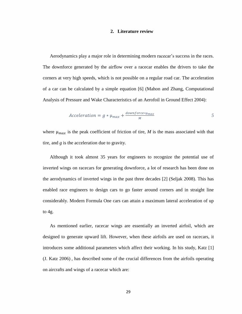
𝐴𝑐𝑐𝑒𝑙𝑒𝑟𝑎𝑡𝑖𝑜𝑛 = 𝑔 ∗ µ𝑚𝑎𝑥 +𝑑𝑜𝑤𝑛𝑓𝑜𝑟𝑐𝑒∗µ𝑚𝑎𝑥
𝑀 5
where µ𝑚𝑎𝑥 is the peak coefficient of friction of tire, M is the mass associated with that
tire, and g is the acceleration due to gravity.
Although it took almost 35 years for engineers to recognize the potential use of
inverted wings on racecars for generating downforce, a lot of research has been done on
the aerodynamics of inverted wings in the past three decades [2] (Seljak 2008). This has
enabled race engineers to design cars to go faster around corners and in straight line
considerably. Modern Formula One cars can attain a maximum lateral acceleration of up
to 4g.
As mentioned earlier, racecar wings are essentially an inverted airfoil, which are
designed to generate upward lift. However, when these airfoils are used on racecars, it
introduces some additional parameters which affect their working. In his study, Katz [1]
(J. Katz 2006) , has described some of the crucial differences from the airfoils operating
on aircrafts and wings of a racecar which are:

30
The racecar wings operate in a strong ground effect as compared to airplane
wings.
The racecar wings have very small aspect ratio.
The overall efficiency of a racecar is greatly affected by the strong
interactions between the wing and other vehicle components.
Where, aspect ratio (AR) is defined as a ratio of wing span to its chord length.
Over the years, a lot of research has been carried out to determine the effects of various
factors to make optimum use of racecar wings. Based on the research conducted, the
overall aerodynamics of the car can be divided into three main categories as:
a. Flow over the front wing
b. The under-body flow
c. Flow over the rear wing
2.1. Front Wing
Front wings first appeared in Formula One just two weeks after the first rear wings
were introduced on Lotus 49B. Since then, it has undergone tremendous modifications
and improvements. The front wing of a modern Formula One racecar is particularly
important as it generates about 30% of the total downforce [2] (Seljak 2008). In addition,
as the front wing is the first part of the car which meets the free stream airflow thus
determining the flow over the rest of the car and the underbody flow, it has been a
favorite topic of research for most of the research done in this field.
31
Realizing its significance, throughout the years, a lot of research has been carried out
on the front wing of a Formula One racecar. Researchers have conducted studies in three
distinguish areas which affect its downforce generating capability; operating in proximity
to ground, effect of incidence or angle of attack and effect of Reynolds number.
2.1.1. Effect of ground clearance on single element front wing
During its initial years, a single element front wing was used on racecars to generate
downforce and would usually be used in small ground clearances. As years progressed,
researchers found that front wing when used at certain ride heights generates more
downforce with less penalty on drag. This was a new phenomenon as the conventional
airfoils were never have been used in such strong ground effects. Numerous studies were
carried by researchers throughout the world and it was found that when operating at
certain ride heights depending on chord length, increased downforce is created.
Continued research indicated that, if the ride height is lowered further, a maximum
downforce is attained after which the downforce decreases. To explain this phenomenon
of effect of varying ground clearance, some of the work conducted in this field was been
reviewed and is stated in this section. In his study, Aerodynamics of Racecars [1] (J. Katz
2006), Katz explained the effect of various ways to generate aerodynamic downforce for
racecars and methods to evaluate the vehicle aerodynamics. The various methods to
generate aerodynamic downforce were use of racecar wings, small aspect ratio wings,
interactions between wing and vehicle, Gurney flaps, creating downforce with the help of
vehicle’s body, diffusers, vortex generators, spoiler, etc. The author has described the
characteristics of racecar wings in particular, front wing when used in ground effect. The

32
author also states that decreasing ground clearance has a positive effect on downforce.
Downforce is increased as the ground clearance is reduced particularly in when it is less
than the airfoil quarter chord. Since, most racecars operate in the ground clearance of H/c
0.1 to 0.3, this phenomenon is widely used in modern racecars. However, this also
increases the induced drag for which to overcome cars need more horsepower. In
addition, since in real world wings operate in a close proximity to ground, the type of
boundary conditions strongly affects both experimental and numerical results. Hence, to
get more realistic results, the importance of moving ground simulation was discussed. In
the study, Katz also discussed the effective use of wind tunnel testing and computational
fluid dynamics (CFD) along with track testing. He suggested that CFD is certainly an
emerging testing method which when used properly will yield credible results for
determining vehicle’s aerodynamic efficiency. He also mentioned, a similar effect of
ground was observed for three-dimensional cases with finite wings and small aspect ratio
(AR=2 rectangular wings).
Another similar study, Racecar Aerodynamics was conducted by Seliak [2] (Seljak
2008), where he described the aerodynamic characteristics of the rear and front wing, and
the underbody flow. In the study, he stated 30-35% of total downforce is created by the
rear wing and about 25-30% by the front wing. The author also stated that elliptical wings
are more efficient to use than rectangular wings and were introduced in the same year as
Gurney flaps were introduced. Over the years, after the fateful incident at Imola in 1994,
the FIA introduced strict rules, which gave rise to the innovation of curved front wings.
This innovation greatly improved the efficiency of the front wing and the underbody flow

33
and thus consolidated the importance of front wing has in determining the overall airflow
over the vehicle body, rear wing and the underbody flow.
Furthermore, a computational study on the front and rear wing of a Formula Mazda
racecar was conducted by Kieffer, Moujaes and Armbya [6] (Kieffer, Moujaes and
Armbya 2004) using the Star-CD CFD package. A standard single element Formula
Mazda front wing was selected for the study, which had a chord of 15 in. The Reynolds
number used were 0.9 x 10⁶ and 1.5 x 10⁶ which corresponded to a reference velocity of
80mph and 130mph respectively. The RANS governing equations were used with the
standard k- ε model as turbulence model. The effect of range of ground clearance and
angle of attack was investigated on both the front and rear wing. The front wing’s
performance seems to be affected by the existence of the ground nearby. The front wing
seemed to develop a larger net downforce (negative lift) when flow was simulated with
ground effect. The calculated results clearly showed an increase in this force when the
front wing was considered with ground effect of about 13% to 20%. This increase was
attributed to the anticipated velocity increase on the underside of the wing, which in turn
decreased the pressure on the wing from that side. The results from the study clearly
show the increase in velocity and pressure in ground effect when compared to freestream
case.
Because of its significance, Ranzenbach and Barlow to determine the effect of ground
clearance on the wing, conducted a series of studies [7, 8, 9] (Ranzenbach and Barlow
1994) (Ranzhanbach and Barlow 1997) (Ranzenbach, Barlow and Diaz 1997) on the front
wing of a racecar. Both experimental and numerical studies were carried out on a single
element front wing using a symmetric NACA 0015 and a negatively cambered NACA
34
4412 airfoils. The authors conducted a two-dimensional study for all the studies as there
exists large quasi two-dimensional flow at the center of the wing when the ground
clearance is very small compared to the wingspan and a stationary ground was used. In
addition, for all the three studies, the angle of attack was kept constant at zero degree and
Reynolds number of 1.5x10⁶ based on chord length which approximately represents a
reference velocity of 100mph was selected. Apart from studying the effect of ground
clearance on the performance of the front wing, the other objective of these studies was
also to determine the capability of the Reynolds Averaged Navier Strokes (RANS)
equations to yield creditable results as there exists some well-known difficulties with the
Ground Floor Boundary Layer (GFBL) for wind tunnel testing which are problematic.
Furthermore, two turbulence models were used, k- ε turbulence for majority of the
study and the one equation k-l turbulence model for the near wall viscous sublayer.
Ranges of ride heights were studied and it was found that the numerical results matched
with experimental results validating the ability of RANS equation to successfully yield
creditable results. It was observed for all the studies that lift behaves as a function of
ground clearance, i.e. lift increases as ground clearance decreases. This phenomenon is
observed at heights approximately 30% to 10% chord length of airfoil. The downforce
reaches a maximum and then decreases as the height is further lowered. This is known as
the force reversal phenomenon, which authors states occur at very small ride heights
usually, less than 10% chord length or less than thickness of airfoil. The reason for the
force reversal phenomenon is stated by the authors was, the merging of ground plane and
airfoil boundary layers and the associated velocity and pressure fields generated between
the two surfaces. It is also stated that this force reversal is a completely viscous
35
dominated phenomenon and is not appropriate for study by boundary layer. It was
further, that the force reversal phenomenon occurs at ground clearances larger for
negatively cambered NACA 4412 airfoil than the symmetric NACA 0015 airfoil.
Mokhtar conducted a similar numerical study [10] (W. A. Mokhtar, A Numerical
Study of High-Lift Single Element Airfoils With Ground Effect For Racing Cars. 2005)
on front wing of a Formula One car using four different airfoils, LNV109A designed by
Lieback, EA23 designed by Eppler, S1223 designed by Selig and Guglielmo and a high
chambered four digits NACA 9315 airfoil, to determine the effect of angle of attack,
Reynolds number and ground clearance on the downforce and drag generated. To
determine the suitable ranges of angle of attack and Reynolds number, a primary study
was conducted in freestream using panel code method XFOIL developed by Drela. Based
on that, the ranges for Reynolds number starting from 0.6 x 10⁶ to 3.6 x 10⁶, angle of
attack from 6.0 to 12.0 degrees and ground clearance (H/c) 0.2 to 1.2 was chosen. The
main study was however, conducted using CFL3D developed by NASA Langley
Research Center. The computational domain of five times was selected and wall with no
slip boundary condition was given to both airfoil surface and ground. A moving ground
and the Menter’s k-ε Shear Stress Transport (SST) turbulence model was used for all the
cases in the study. A high and medium ground clearance were studied and found out that
for medium ground clearance, a considerable increase in downforce can be gained by
even small decreases in ground clearance. For medium ground clearance, both lift and
drag increases as ground clearance is decreased and an average increase in downforce by
decreasing ground clearance from H/c 0.6 to 0.2 is 30%. However, its effect on lift is
limited to ground clearance less than 60% chord length.

36
Another study [11] (Mokhtar and Lane, Racecar Front Wing Aerodynamics 2008) to
investigate the behavior of front wing with a small ground clearance was conducted by
Mokhtar and Lane using CFD code Star CCM+ for simulation of a racecar front wing. A
symmetric NACA0012 wing was used for a constant angle of attack of 6 degrees and
Reynolds number of 1.5 x 10⁶. It was found out that as the ground clearance decreases,
the wing generates more downforce. The peak value of downforce was observed at 10%
ground clearance. The wing generated less downforce when performing at ground
clearance less than 10%. The generated drag has a similar trend with its peak at 8%
ground clearance. The study also showed that the lower surface of the wing plays the
major role in controlling magnitude of the generated forces for a wing with a small
ground clearance. As the ground clearance gets smaller, the effective angle of attack of
the wing increases and causes the separation on the lower surface and ultimately cause a
stall like phenomenon for ground clearance less than 10%. The span wise load
distribution of the wing is affected by the ground clearance less than 8%. The wing
generates a smaller wake and weak wingtip vortices at small ground clearance.
The same author conducted a study [12] (W. A. Mokhtar, Aerodynamics of High-Lift
Wings with Ground Effect for Racecars 2008) where the aerodynamics of finite-span
rectangular wing was studied using numerical method. A high-lift single element airfoil
section was used and study for effect of ground clearance was carried out. Two wings
were studied, with and without end plates and the CFD code of Star CCM+ was used for
the study. The paper focused on the study of effect of ground clearance for three-
dimensional flow of S1223 wing with and without the end plates. The height of end
plates selected was half the chord length on both sides of the wing. Angle of attack at 6

37
degrees and Reynolds number, Re = 1.5 x 10⁶ were kept constant. For the study, a
segregated three-dimensional flow was selected to solve for RANS equations and Gauss-
Seidel relaxation scheme was used along with k-epsilon two equation turbulence model.
The computational domain selected was ten times the chord length and half wing was
used for simplicity. Wall boundary condition was given with no slip effect and moving
ground was used. For reference point, the flow in no ground effect was studied and was
found that air reaches a maximum velocity about 53% higher than freestream velocity in
lower surface. Furthermore, it was found that for finite-span wing, wing tip vortices are
created which cause a decrease in downforce and increase in induced drag, which
ultimately results in more wake deformation. For small ground clearance H/c = 0.2, the
maximum velocity is 130% more than freestream velocity and generates more downforce
and drag. Also, it was found that it delayed the development of wing tip vortices and
were weaker than the free flow case. For very small ground clearance H/c = 0.1, negative
downforce is generated as the flow is blocked by a thicker boundary layer due to
merging. For medium ground clearance H/c = 0.6, the maximum velocity was 93% more
than the freestream velocity and has less effect on downforce. In addition, the wing tip
vortices were well developed than small ground effect. For medium ground clearance,
less than 60% of chord length, considerable amount in increase in downforce can be
achieved which is the normal operating ground clearance for racecar wings.
A CFD simulation of the high lift single element airfoil S1223 for racecar front wing
in ground effect was carried out in STAR CCM+ again by Mokhtar [13] (Mokhtar and
Durrer, A CFD Analysis of a Race car Front Wing in Ground Effect 2016). The wing was
tested in different level of ground clearance from H/c = 0.15 to 0.5 of leading edge with a

38
constant angle of attack of 6 degrees and Reynolds number of 0.6 x 10⁶. The reference
velocity of 30m/s was chosen corresponding to the cornering speeds in Formula One. For
the study, a segregated three-dimensional flow was selected to solve for RANS equations
and Gauss-Seidel relaxation scheme was used along with k-omega two-equation
turbulence model. The computational domain selected was ten times the chord length and
half wing was used for simplicity. Wall boundary condition was given with no slip effect.
Depending upon the ground clearance, 6 to 10 million cells were used. It was found that
as the ground clearance decreases, the coefficient of lift increases up to a maximum point
of H/c =0.22. The flow structure analysis indicated an increase of velocity between wing
and ground while decreasing the ground clearance, which also lead to a stronger suction.
Furthermore, by observing the wake, analysis showed that in ground effect, multiple
span-wise vortices start to build and get stronger with decreasing ground clearance.
Figure 4 and Figure 5 shows the wake velocity distribution on the front wing in varying
ground clearances.
Figure 4: Wake velocity distribution on a plane 2/3 of a chord downstream at a ground
clearance H/c=0.3 (Mokhtar & Durrer, A CFD Analysis of a Racecar Front Wing in
Ground Effect, 2016)

39
Figure 5: Wake velocity distribution on a plane 2/3 of a chord downstream at a ground
clearance H/c=0.22 (Mokhtar and Durrer, A CFD Analysis of a Race car Front Wing in
Ground Effect 2016)
Moreover, the continuous drag increase showed the effect of increasing skin-friction
drag and induced drag through wake. This generates a negative downforce as the ground
clearance decreases.
As mentioned earlier, to get more realistic results, the importance of moving ground
simulation was realized and researchers found new ways to conduct such studies.
Keeping this in mind, a series of both experimental and numerical studies were conducted
by Zerihan and Zhang on single and multi-element front wing of a Formula One racing
car. In their first study [14] (Zerihan and Zhang, Aerodynamics of a Single Element Wing
in Ground Effect 2000), Zerihan and Zhang conducted an experimental study of a single
element front wing of a Formula one racing car in varying ground clearances and angle of
attacks. The airfoil selected for study was a highly cambered single element Tyrelle 026
Formula One front wing which was a modified NASA GA(W) profile of type LS (1)-
0413 of span 1100mm, chord of 223.4mm and an aspect ratio of approximately equal to
5. Rectangular end plates were attached to the wing model. The reference velocity of

40
30m/s was used for a Reynolds number of roughly 2 x 10⁶ based on chord length. The
effect of varying ground clearance and angle of attack was studied for a moving ground
boundary condition. It was found that for freestream case, the lift coefficient reached a
maximum of 1.35. However, when studied for varying ground clearances, lift behaves as
a function of ground clearance and the lift coefficient reached a maximum of 1.72 at a
ride height of 0.08c. Furthermore, the drag also increases as ground clearance decreases.
The authors specified this by stating that, as ride height is reduced the induced drag
increases, which in turn increases the overall drag, produced. In addition, due to
separation of boundary layer at the trailing edge for ground clearances lower than the
maximum lift, drag is increased. For ride heights, lower than 0.08c, the force reversal
phenomenon was observed. The authors stated that, this force reversal phenomenon is a
result of separation of boundary layer at the trailing edge of the wing and not due to the
merging of boundary layers. The height at which force reversal occurs is due to a
combination of minimum loss of downforce due to separation of boundary layer and
maximum gain in lower surface suction due to small ride heights. On the other hand, the
separation of boundary layer at the trailing edge occurs due to the boundary layer not
being able to withstand the adverse pressure gradient associated with highly accelerated
flow at small ride heights.
A computational study [15] (Mahon and Zhang, Computational Analysis of Pressure
and Wake Characteristics of an Aerofoil in Ground Effect 2004) on the same wing model
with rectangular end plates was conducted by Mahon and Zhang to study the influence of
individual turbulence models using Reynolds Averaged Navier Strokes (RANS) equation
simulation and wind tunnel measurements. A total of six turbulence models were used

41
viz., one equation Spalart-Allmarus, the standard k- ε model, the standard k- ω model, the
standard k- ω SST model, the k- ε RNG model, and the Realizable k- ε model. To save
computational time and as quasi- two-dimensional flow exists in the mid span of wing, a
two-dimensional study was carried out. The RANS equations were solved using
SIMPLEX solver for a two-dimensional steady state segregated flow. A moving ground
simulation was selected and the ground and airfoil were defined as wall with no slip
boundary condition. Reference velocity of 30m/s was used with a turbulent viscosity ratio
of 10. For the study, two ride heights were investigated, 0.224c and 0.09c, representing
the force enhancement and force reversal phenomenon respectively. Results from both
wind tunnel and computational method were compared and investigated. It was found
that the RANS equations were successfully able to generate credible results. Table 1
shows the results from both wind tunnel and computational method using all turbulence
models. Furthermore, for ride height of 0.224c, all the turbulence model performed well
and it was observed that, the separation region starts to appear at the trailing edge.
However, for the ride height of 0.09c, k- ω SST model gave the best results and the
reduction in downforce was correctly predicted by it whereas, the Realizable k- ε model
failed to predict it. Hence, it was suggested k- ω SST model is best used for predicting
surface pressures and sectional forces while the Realizable k- ε model is best for
predicting wake flow field, especially in lower wake boundary. The Table 1 shows the
application of the Realizable k- ε model and k- ω SST turbulence models predicting the
wake generated at various heights.

42
Table 1: Realizable k- ε model and k- ω SST turbulence models predicting the wake at
various heights. (Mahon & Zhang, Computational Analysis of Pressure and Wake
Characteristics of an Aerofoil in Ground Effect, 2004)
Zhang also conducted a numerical study [16] (Kuya, et al. 2009) to investigate the
flow separation control on a racecar wing with vortex generations in ground effect. The
study was carried out to investigate the effect of flow separation control vortex when
used on a single element inverted wing over a range of ride heights and angle of attack.
Counter rotating and co-rotating rectangular vane type vortex generators were studied on
the suction surface of the wing. Particularly the effect of device height and spacing was
investigated in the study. The airfoil selected for the study was the same a highly
cambered single element Tyrelle 026 Formula One front wing with endplates. A
reference velocity of 30m/s was used which corresponds to a Reynolds number of
roughly 450,000 based on chord length. To save computational time and as quasi- two-
dimensional flow exists in the mid span of wing, a two-dimensional study was carried
out. It was found that the counter rotating sub-boundary layer vortex generators yields a
26% improvement in the maximum downforce generated at low ride heights and a 10%
improvement in the lift to drag ratio indicating an overall improvement in the
h/c Expt/CFD u min /U ∞ y/c at u min
Expt 2.617 0.071
Real k- ϵ 613 0.074
k-ω SST 0.591 0.073
Expt 0.525 0.061
Real k- ϵ 0.529 0.065
k-ω SST 0.507 0.063
Expt 0.35 0.031
Real k- ϵ 0.405 0.054
k-ω SST 0.367 0.049
0.448
0.224
0.134

43
aerodynamic efficiency of the wing. However, both the vortex generators indicate a
suppression of boundary layer separation at the trailing edge. In the end authors
suggested that, counter rotating sub-boundary layer vortex generator is effective in
controlling flow separation and thus providing an improvement in downforce with a
relatively low drag penalty.
A numerical study was conducted by E. Genua [17] (Genua 2009) to investigate the
effect of ground clearance on an inverted two-dimensional airfoil. The study also
investigated the applicability of different turbulence models to predict the separation of
boundary layer at the trailing edge experienced in ground effect. To save computational
time and simplicity, a two-dimensional computational study was conducted. The airfoil
used was the same single element airfoil used by Zerihan and Zhang for their series of
studies. An angle of attack of 3.6 degrees was kept constant with a constant Reynolds
number of 4.5 x 10⁶ based on chord length with corresponds to a free stream velocity of
30m/s. The Reynolds Averaged Navier-Strokes equation were used with a moving
ground simulation. A wall boundary condition with no slip was defined for airfoil and
ground. For meshing a growth factor of 1.1 to 1.2 was used. In this study the three
different turbulence models used were one equation Spalart-Allmarus, the standard k- ω
SST model and the Realizable k- ε model. To study the effect of ground clearance two
different ride heights were studied which were 0.224c and 0.09c. In addition, both steady
and unsteady state simulations were investigated. However, the results did not show
considerable differences between the steady and unsteady state simulations. In the study,
it was found that all the turbulence models could accurately predict the flow for the free
stream case. On the other hand, for ride height of 0.224c and freestream case, the
44
standard k- ω SST model gave the best results and the values matched well for downforce
and drag from previous experimental study conducted by Zerihan and Zhang [14]
(Zerihan and Zhang, Aerodynamics of a Single Element Wing in Ground Effect 2000).
Furthermore, for the ride height of 0.09c, the one equation Spalart-Allmarus, could
accurately predict the large separation of boundary layer at the trailing whereas, the
standard k- ω SST model and the Realizable k- ε model had difficulties in the same.
Hence, it was suggested that the one equation Spalart-Allmarus is the best turbulence
model to study the effect of ground clearance on an inverted single element wing.
Another similar study was conducted by Price [18] (Price 2011), to investigate
the ability of Fluent 6.3 and the Realizable k- ε model to depict the flow over a front wing
of a racecar in interaction with its front wheels. The study focused on assessing the
effects of ground clearance, wing-wheel interaction and wing tip vortices, each of which
has a significant effect on the efficiency of a front wing for an open wheel racecar. For
the study, a front wing of Cal. Poly’s 2008 Formula SAE car was used which was a FX
63-137 wing with a 0 degree angle of attack, span of 0.635m and a chord length of
0.433m. The numerical study was carried out in Fluent 6.3 which makes use of RANS
governing equations and a SIMPLEX algorithm for a steady state case. As stated, the
Realizable k- ε model was used for turbulence for a freestream velocity of 18m/s. A solid
model of the wing stated was created using SolidWorks and symmetry was for simulating
half the car to save computational time. Mesh was created using 4.5 million tetrahedral
cells using prism layer with a growth factor of 1.2. The computational domain of about 4,
4 and 6 car lengths was created in the front, above and back of the car respectively with a
width of about 3 car lengths from the axis of symmetry. A total 800 iterations were

45
carried out to converge the momentum and energy governing equations. Initially, the
study aimed at validating the computational results by conducting an experimental study
by examining the lap times of the SAE racecar. However, due to failures caused to
engine, the results were not validated experimentally. On the other hand, the results from
computational study showed that governing equations for turbulence with the use of the
Realizable k- ε model, converged to the order of 10-3 and 10-6. In addition, by studying the
wing in varying ground effect, the results also showed that, mounting the wing in 10%
chord length from ground the suction peak increased by about 278% which ultimately
gave rise to an increase in downforce generated.
Thus, to conclude, ground clearance has a significant impact on the overall
aerodynamic efficiency of the front wing of a racecar and designers should take into
considerations its effect to determine optimum operating conditions during a race. The
effect of ground clearance could be broadly divided in two areas, a downforce
enhancement region where lift behaves as a function of ground clearance for medium
ground clearances and a force reversal area where for very small ground clearances
downforce reduces after reaching a maximum as ride height is lowered.
2.1.2. Effect of varying angle of attack
The angle of attack or incidence is defined as the angle between the chord line of
the airfoil and the direction of flow. The effective camber of an inverted wing is
increased when its angle of attack is increased. This in return helps in achieving a higher
maximum coefficient of lift. Hence, by increasing the angle, downforce generated can be
increased and a maximum downforce is reached at certain angle of attack. However, after

46
the maximum downforce is reached, any further increment results in separation of flow at
the trailing edge due to formation of a thick boundary layer. This effect of varying angle
of attack has been reviewed through works of different authors and is explained in this
section.
Katz [1] (J. Katz 2006) in his study has described angle of attack as one of the
prime parameters which affect the aerodynamics of a front wing significantly. Seliak also
in his study [2] (Seljak 2008), has described the significance of angle of attack. He
mentioned, designers always strive to develop wings with higher maximum coefficient of
lift and a way to achieve this is to make use of highly cambered airfoils. However, due to
strict regulations by racing governing bodies, designers are restricted to use very high
cambered airfoils. As a result, designers found a way to deal with this situation. Through
the research conducted over the years, it was noticed that the camber of an airfoil can be
increased considerably if the angle of attack is increased. This is return leads to a higher
value of maximum coefficient of lift and thus more downforce is created.
In the study of Formula Mazda racecar [6] (Kieffer, Moujaes and Armbya 2004)
as mentioned earlier, the effect of varying angle of attack was also studied.
The results showed that there was a slight increase in the Cl of about 20% from 0
degree to 12 degrees of angle of attack when ground effect was considered. In addition,
there was a marked decrease in Cl by about 45%, which may indicate that between 12
degrees and 16 degrees of angle of attack, there is a potential for a stall condition with the
airfoil. Also, the Cd for that wing showed a steady increase to about 50% until the 12
degrees of angle of attack was reached, after which the value of the coefficient value
becomes relatively constant.

47
As mentioned earlier, Mokhtar [10] (W. A. Mokhtar, A Numerical Study of High-
Lift Single Element Airfoils With Ground Effect For Racing Cars. 2005), conducted a
numerical study focused on the study of high-lift airfoils suitable for racecar applications.
In this study, the effect of ground clearance, angle of attack and Reynolds number based
on airfoil chord length was determined. It was found that; angle of attack differs linearly
for medium ground clearance and medium Reynolds number. The high camber with high
angle of attack generated significant downforce. However, a boundary layer develops and
eventually becomes thick enough to cause separation of flow at high angle of attacks.
Furthermore, for low angle of attack i.e. 6 degrees and medium Reynolds number i.e. 1.2
x 106, the larger ground clearance does not have any effect and is like freestream flow.
Similarly, as mentioned earlier to investigate the effect of angle of attack on a
single element front wing of a Formula One racecar in ground effect, a study was
conducted by Zerihan and Zhang [14] (Zerihan and Zhang, Aerodynamics of a Single
Element Wing in Ground Effect 2000). In their study, they investigated the aerodynamics
of mentioned inverted wing over a range of angle of attacks from -10 degrees to 25
degrees. The wing was rotated about a point at 0.25c from the leading edge. It was found
that a maximum downforce is achieved for angle of attack of 11.3 degrees. At this angle,
a separation of boundary layer at trailing edge is also observed. The study also indicated a
reduction in downforce at an angle of 18.4 degrees. The authors stated that, the
downforce increases as the angle of attack is increased and an increase in angle of attack
also decreases the sensitivity of downforce to ride heights. However, for high values of
angle of attack, the force reversal phenomenon occurred at higher values of ground
clearance.

48
In the same study Zerihan and Zhang, investigated the effect of simultaneously
varying the ground clearance and angle of attack on the inverted single element front
wing. A range of -3 degrees to 11 degrees is selected due to the restrictions imposed on
angle of attack using end plates. Thus, no force reversal is observed.
Therefore, to conclude, it can be stated that, downforce increases with an
increasing angle of attack as it increases the camber of the wing. It reaches a maximum
creating a thick boundary layer causing separation at the trailing edge, which eventually
results, is reduction in downforce for any further increase in angle of attack.
2.1.3. Multi-element
Throughout the years’ researchers and designers have found innovative ways to
increase the maximum downforce generated by racecar wings. One of the most effective
ways to generate downforce identified was to make use of multi-element wings. The first
multi-element wings were introduced by McLaren in 1984 and since then they have been
used regularly in most of the racecars. The regulations allow the angle of attack of the
second element or flap to be modified so that the load applied on the front wing could be
changed to balance the car according to various conditions [2] (Seljak 2008).
Acknowledging the importance of multi-element wings, an experimental study
was conducted by Jasinski and Selig [19] (Jasinski and Seilg 1998), on front wings of an
open wheel racecar. The airfoil selected for the study was a two-element UIUC 700
airfoil with endplates. The main element and flap had chords of 22.86cm, 10.16cm
respectively with a total chord of 33.02cm. Endplates were attached, and the span of the
49
wing was of 46.23cm. The effect of varying ground clearance, angle of attack and
Reynolds number was investigated. It was observed that negative lift or downforce
increased as the Reynolds number was increased with a simultaneous reduction in drag.
When the flap angle was varied, it was noted that the downforce increased with
increasing angle with no appreciable change in the overall drag. Moreover, the wing
showed same effect when the planform area of flap was increased.
To study the multi-element airfoil in ground effect, Ranzenbach, Barlow and Diaz
conducted a study [9] (Ranzenbach, Barlow and Diaz 1997). In this study, they studied a
negatively cambered two-element single slotted 30% chord flap NACA 632-215 Mod B
airfoil experimentally and numerically. A two-dimensional study was conducted as along
the mid span region a quasi-two-dimensional flow exists and it saves computational time.
A total of five ride heights were studied with a stationary ground simulation. A constant
angle of attack of 0 degree was used for a Reynolds number of 1.5 million based on chord
length. It was found for ride heights roughly equal to the thickness of the airfoil, the
downforce behaves as a function of the ground clearance. In addition, the force reversal
phenomenon occurs at heights larger then both the symmetric NACA 0015 and
negatively cambered NACA4412 airfoils in the studies conducted by same authors [7]
[8]. The height that the force reversal occurs is less than 22% of chord length of airfoil.
The authors state the occurrence of force reversal due to the merging of boundary layers,
and velocity and pressure fields generated between the two surfaces.
Zerihan and Zhang, also conducted a series of studies on the multi-element front
wing of a Formula One racing car to determine its aerodynamic behavior in ground effect
and varying flap angles. They conducted experimental and computational studies on a

50
high lift cambered double element Tyrelle 026 Formula One front wing which was a
modified NASA GA(W) profile of type LS (1)-0413. A study [20] (Zhang and Zerihan,
Aerodynamics of a Double-Element Wing in Ground Effect 2003) was conducted to
investigate the effect of ground clearance and to quantify the optimum flap setting. The
wing model for all the studies consisted of a main element of chord 223.4mm and a flap
of chord 165.7mm with a combined chord of about 380mm. The wing had a span of
1100mm with an aspect ratio of 2.89. Reynolds number of 7.35 x 10⁵ to 7.65 x 10⁵ based
on chord length is used which corresponds to a freestream velocity of 30m/s. Two flap
angles were studied and the flap was rotated at about 0.567c from the leading edge. In the
experimental study, different gap and overlap settings were used to determine the
optimum location for flap. It was found that for optimum flap setting, the gap and overlap
should be 0.024c and 0.032c from the leading edge respectively. It was also found that
the flow is three dimensional towards the wing tip and that most of the downforce is
generate by the main element. The main element not only generates most of the
downforce but also, dominates the turbulent wake generated by the wing. On the other
hand, the variation in ground clearance has no effect on the turbulent wake generated
from the flap. It was observed that as ground clearance is reduced the boundary layer gets
thicker in the suction surface of main element, which cause an increase in both wake
thickness and a reduction in the velocity deficit. Furthermore, three distinct regions were
observed when the ride height of wing was reduced.
It is observed that, for large ride heights, the downforce increases asymptotically
with reduction in height. Then for low flap angles, the downforce reaches a plateau and
for high flap angles, a reduction in downforce is noted. The second region exist for

51
medium ride heights where the downforce reaches a maximum value and the third region
exists for small rides where a force reversal region like the single element force reversal
is observed. It was also noted that for high flap angle scenario the drag and lift were
generated by the not only by main element but also by the flap unlike the low flap angle
case.
Also, as a part of the series of studies on multi-element front wing, Mahon and
Zhang conducted a computational study on an inverted double element front wing [21]
(Mahon and Zhang, Computational Analysis of an Inverted Double-Element Wing in
Ground Effect 2006). They investigated the effect of ground clearance on a double
element wing with the same airfoil mentioned above. A two-dimensional study was
conducted and the efficiency of six turbulence models was determined. The six
turbulence models used were one equation Spalart-Allmarus, the standard k- ε model, the
standard k- ω model, the standard k- ω SST model, the k- ε RNG model, and the
Realizable k- ε model. A reference velocity of 30m/s was used which corresponded to a
Reynolds number of 7.86 x 10⁵ based on chord length. Two different ride heights of
0.211c and 0.079c were studied which represented the force enhancement and force
reversal regions respectively. It was observed that, all turbulence models could predict
the flow over the wing in good agreement with the Realizable k- ε model yielding the best
results. Moreover, as observed in experimental study, the majority of downforce was
generated by the main element and the flap generated the majority of drag. It was also
noted that the main element wake beneath the flap suction surface spread at an increased
rate with reducing ride heights. Furthermore, the main element finite trailing edge and the
corresponding downstream circulation region generated most of the main element wake,

52
and it was proposed by the authors that by use of sharp trailing edge for main element, its
wake can be reduced. The authors also stated because of lack of three-dimensionality, the
vertical location of the lower boundary of main element was unpredicted and could be
improved by use of finite span wings.
Zerihan and Zhang conducted another experimental study investigating the effect
of edge vortices generated by a double-element front wing on forces [22] (Zhang and
Zerihan, Edge Vortices of a Double-Element Wing in Ground Effect 2004). The same
double-element front wing as discussed in previous studies was used in this study. From
the results, it was concluded by the authors that the flow near the tip for main element is
mostly three-dimensional. In addition, the downforce generated near the tip of main
element is significantly less than that of in the center. Furthermore, the curve of total
downforce vs. ride height showed three distinct regions. The first region comprised of
force enhancement and concentrated edge vortices where the flap produced more
downforce at tip than at its center. The second region consisted of force enhancement and
vortex breakdown where the vortex breaks down which results in a loss of downforce at
the tip of flap ultimately changing the curve of downforce. In both these regions, the
force enhancement implies downforce increases as ride height is lowered. The third
region comprised of loss of downforce and separation on the wing, which has been
explained by the authors in previously mentioned studies.
Thus, to conclude the multi-element wings are used to generate significant
amount of downforce with less penalty on drag. Most of the total downforce is generated
by the main element while the flap is responsible for generating most of the total drag. In
addition, depending on the flap angle the contribution of flap varies. However, there still

53
exist a need to conduct a three-dimensional study of multi-element front wing in ground
effect to get a clearer understanding.
2.1.4. Gurney flaps
In 1971, earlier first improvement was also made to front wing with the use of
Gurney flaps. Gurney flaps were developed to reduce the drag and these are small
vertical reinforcement mounted on the top of airfoil, at the trailing edge, spanning the
whole width [1]. Since its introduction, Gurney flaps have been regularly used in racecars
and in airplanes widely to increase the overall efficiency of the wings.
As a part of series of studies conducted, Zerihan and Zhang conducted a study
[23] (Zerihan and Zhang, Aerodynamics of Gurney Flaps on a Wing in Ground Effect
2000) to investigate the effect of Gurney flap on a high lift, single-element front wing in
ground effect. The effect of Gurney flap in terms of the aerodynamic and flow
characteristics was determined. A high-lift, single-element front wing in ground effect
was used for this study and the airfoil used was the same used by the same authors in
previous studies as [14] (Zerihan and Zhang, Aerodynamics of a Single Element Wing in
Ground Effect 2000). A freestream case was also investigated and was found that the
normal force on the wing was increased resulting in sharper stall. The effect of small and
large Gurney flaps was studied in ground effect. It was observed that for medium ground
clearance of force enhancement regions, the Gurney flap increases the downforce
generated. It was noted that, Gurney flap yields more downforce when used in ground
effect than in freestream. By studying the turbulent wake behind the wing, it was
observed that for low ride heights, as the flow starts to separate from the trailing edge of

54
the suction surface, a stall is developed when ground clearance is lowered and an
unsteady wake is generated which results in deterioration of aerodynamic performance of
Gurney flaps. Also, large Gurney flaps proved more efficient than smaller ones.
2.1.5. End plates
One of the key differences between a conventional airfoil and racecar wings is,
racecars are finite wings. This leads to formation of end tip vortices which create an
induced drag thus, increasing the overall drag generated. Endplates have been by racecars
to cope up with this drawback since last few decades. Even though endplates are used on
front wings, when used in ground effect, most of the end tip vortices are nullified by the
ground. Hence, few studies have been conducted to study to the effect of endplates on the
front wing as it has a minimal effect. Said that, the following section reviews the effect of
endplates on the front wings.
Katz in [1] (J. Katz 2006) states that modern racecars still make use of wings with
aspect ratio, AR = 2 and due to the traditional finite wing effect, these wings experience a
change in pressure distribution than high aspect ratio wings. However, this can be
encountered by pitching the wings more to increase the leading-edge suction. However,
in real conditions, there occurs a local trailing edge separation, which is reduced by the
two strong side vortices. In addition, the end plates (or side fins) also have a positive
effect with smaller drag increment and thus having higher lift to drag ratio.
Mokhtar conducted a study [12] (W. A. Mokhtar, Aerodynamics of High-Lift
Wings with Ground Effect for Racecars 2008) where the aerodynamics of finite-span
55
rectangular wing was studied using numerical method. A high-lift single element airfoil
section was used and study for effect of ground clearance was carried out. Two wings
were studied, with and without end plates and the CFD code of Star CCM+ was used for
the study. The paper focused on the study of effect of ground clearance for three-
dimensional flow of S1223 wing with and without the end plates. The height of end
plates selected was half the chord length on both sides of the wing. Angle of attack at 6
degrees and Reynolds number, Re = 1.5 x 10⁶ were kept constant. For the study a
segregated three-dimensional flow was selected to solve for RANS equations and Gauss-
Seidel relaxation scheme was used along with k-epsilon two equation turbulence model.
The computational domain selected was ten times the chord length and half wing was
used for simplicity. Wall boundary condition was given with no slip effect and moving
ground was used. There was no considerate variation in the behavior of wing with end
plates than those without. For medium ground clearance, less than 60% of chord length,
considerable amount in increase in downforce can be achieved.
2.1.6. Vehicle-wing interaction
An effective way of generating more downforce with less penalty on drag was
discovered in 1977 by introduction of Lotus T78 when they used the so-called side-pods
[2] (Seljak 2008). Lotus made use of an underbody of racecar shaped as an inverted wing
which enabled them to take corners at exceptional high speeds. A huge amount of
downforce was created with reduction in drag by decreasing the gap between ground and
side-pods. As the gap was reduced, the flow beneath the car was accelerated further
creating an additional decrease in pressure on lower surface which led to an increase in

56
downforce. Thus, a new way of creating downforce was discovered which soon was
adapted by other teams. However, the use of side-pods was banned in 1983 after new
restrictions were imposed by FIA.
Another attempt to generate downforce with use of more suction beneath the car
was done by Brabham and Chaparral with the help of fans to suck air under the car, thus
creating a low-pressure region under the car [2] (Seljak 2008) . The Chaparral 2J in 1969
used two rear fans while Brabham BT46 used a rear mounted fan driven by gearbox in
1978. Both racecars proved highly efficient in winning races but were immediately
banned. Thus, the use of vehicle body to generate downforce became evident and
researches started investigating new ways to improve its aerodynamic efficiency.
In open wheel races, such as Formula One and Indy car, the flow behind a front
wing becomes critical as it can drastically reduce the efficiency of the car by interacting
with the wheels and other components. Hence, researches have tried to investigate the
wake characteristics of the front wing and its interaction with the front wheels. One such
study was conducted by Katz, Luo, Mestreau and Baum, and Löhner [24] (Katz , et al.
1998). They conducted a numerical study of an open wheel Indy racecar where they
explained the effect of some of the non-linear effects to shorten the overall design cycle.
The study also investigated the applicability of the computational methods in areas where
experimental studies has limited scope. For the study, the authors generated a model of a
generic Indy racecar with the help of FECAD. Further, the meshing was carried out in
FRGEN3D and the Euler and RANS turbulent equations were solved in FEFLOW97/8
solver. In addition, the results were graphically represented with the help of FEPOST3D.
The study also aimed at investigating the internal flow across the radiator ducts. A proper

57
boundary conditions were given to simulate the real race conditions by rotating the
wheels and a moving ground simulation was conducted to yield accurate results.
Furthermore, a freestream velocity of about 100mph was used for the study. For
turbulence, various turbulence models were selected and the standard k- ε model was
found to give the best results. However, in the study no turbulence was used as data
represented virtually a high Reynolds number laminar flow. From the results, it was
stated that the numerical methods show good potential for use as a complementary tool
for testing and designing. The study also showed, in open wheel racecars, the interaction
of front with front wheels causes a loss of downforce thus decreasing the aerodynamic
efficiency of the car. However, with the help of wing tip vortices the flow behind the
front wing can be directed to away from the wheels and ultimately reducing the losses by
interaction.
Another similar computational study to investigate the wing-wheel interaction
was conducted by Price [18] (Price 2011), with the wing of a 2008 Formula SAE racecar
as mentioned above in earlier section. The study aimed at determining the effect of a
front wing of a racecar in interaction with its front wheel with a varying ground
clearance, wing-wheel interaction and wing tip vortices.
The results from this computational study indicated a high-pressure region in
front of tires as indicated by the red region in Figure above. This high-pressure region
was a result of slowing down of air in the gap between wing and wheel. Also, a
separation of flow occurs due to interaction which causes losses in downforce.
Furthermore, by studying wing tip vortices, it was found that an induced drag is
generated by these vortices which significantly increases the overall drag generated. The

58
author suggested the use of endplates or side-pods as a counter measure to reduce these
wing tip vortices.
However, there are certain areas that still lacks the depth in research to determine
their optimum use. Zhang and Zerihan [25] (Zhang, Toet and Zerihan, Ground Effect
Aerodynamics of Race Cars 2006), reviewed the progress made in past 30 years on
ground effect aerodynamics of open wheel racecars and concluded that the flow around
the wheel is one area in the field which lacks both qualitative and quantitative work.
2.1.7. Wake characteristics
As the front wing is the first part of a racecar which meets the freestream velocity,
it dictates the flow over the vehicle and underbody flow. Thus, it’s critical to have a
relatively less turbulent flow behind the front wing. Researchers have conducted various
studies to determine the wake characteristics behind a front wing to improve the overall
efficiency of a racecar. One of such studies was conducted by Zhang and Zerihan [26]
(Zhang and Zerihan, Turbulkent Wake behind a Single Element Wing in Ground Effect
2004) in their series of studies on single element front wing of a Tyrelle 026 F1 car. This
study aimed at determining the wake characteristics of single element front wing in
ground effect. The wing profile is the same as used in previous studies by same authors
and is mentioned earlier. The study was conducted experimentally at a freestream
velocity of 30m/s corresponding to a Reynolds number of 0.430 – 0.462 x 10⁶. A moving
ground was used with varying heights and an angle of attack of 0o. The wake was
observed at three different locations of about x/c = 1.5, 2.0 and 3.0 downstream from
leading edge. From the results, it was observed that, at large heights a small turbulent

59
wake was generated which moved and grew upwards as it travelled downstream.
Furthermore, at this height a vortex shedding was also observed. In addition, as the height
is lowered, boundary layer separation occurred at the suction side and the turbulent wake
on this side grew due to the separation. Moreover, the low ride heights, the instability of
the shear layers produced large vortices which gave rise to induced drag.
During a race, a racecar would have to operate in the wake of a car in front which
has severe effects on its efficiency. This phenomenon, when a racecar is closely
following another car is also known as drafting. The front wing is mostly affected as it is
the first part which meets the turbulent air generated by the car in front. To study this,
some studies have been conducted by researchers both experimentally and
computationally. In either case, a scaled model or a bluff body depicting the flow of an
actual racecar is used to study the wake characteristics. One such study was conducted by
Wilson, Dominy and Straker [27] (Wilson, Dominy and Straker 2008), examining the
aerodynamic characteristics of a car wing operating in a wake. Both experimental and
computational study was conducted with a goal to examine the wake structure of a
generic Formula One racecar and study its effect on the front wing of a Formula One
racecar with a help of a short bluff body. A 1/6th scaled model was created which
satisfied the 2006 regulations set by FIA for Formula One championship for the
experimental study and a 1/3rd scaled short bluff body was modelled for computational
study which approximately depicted the wake of a regular racecar. Both the experimental
and computational study was conducted with a moving ground simulation at a Reynolds
number of 6 x 10⁵ and the wake was measured at two different locations of x/c = 0.25 and
0.5. To save computational time, symmetry was used and a ½ car simulation was

60
conducted. The single element wing profile used for the study was NASA/Langley LS (1)
– 0417 (GA (W)-1) with a chord of 250mm and span of 600mm equipped with endplates.
The results from both the studies were verified and studied.
It was noted that the wake is dominated by a vortex pair with very high levels of
turbulence which exceeds 40% in places as shown above. The effect of wake on
aerodynamics of the following car however, were described in three categories. These
were a velocity deficit area associated with zones of low stagnation pressures. A region
of high turbulence and an increase in local incidence resulting from stream wise vorticity.
In addition, the front wing of a drafting car experiences a high freestream
turbulence within the wake of the car in front which causes the stall phenomenon to
delay.
Also, it was observed that even though the influence of wake reduces rapidly, the vortex
structure remains more persistent. Furthermore, because of this, the following front wing
experiences a significant increase in local incidence or angle of attack and thus leading to
loss of downforce and increase in drag.
Another similar study, to investigate the effect of drafting was conducted by Soso
and Wilson [28] (Soso and Wilson 2005). In their study, authors created a 40% scaled
model of a 2002 Formula One racecar and studied the effects of drafting on a single
element front wing. The wing selected was a NASA/Langley LS (1) – 0417 (GA(W)-1)
scaled to 40% with a chord of 220mm and span of 550mm equipped with 5mm thick
endplates. A range of ride heights from 2mm to 169.6mm and angle of attack from -50
and 300 pivoted about quarter chord length from leading edge for a Reynolds number of
300,000 to 309,000 based on chord length representing a reference velocity of 20m/s. It

61
was concluded from the results that, when in wake, the drafting wing experienced a loss
of downforce and an increase in drag. It was also noted that, more downforce was lost at
higher heights than compared to low ride heights. Furthermore, more downforce
reduction occurred at areas closer to mid-span than the tips. The load distribution was
also lower in mid-span regions at higher heights which reversed at low ride heights. Also,
the downstream wing was affected by the up-wash flow field from the leading car. An
earlier laminar-to-turbulent transition was also observed on the drafting wing due to
wake.
2.2. Rear Wing
Katz [1] (J. Katz 2006) and Seliak [2] (Seljak 2008) in their study have described that
about 30% to 35% of total downforce is created with the help of the rear wings in modern
racecars. Researchers around through various studies have found that, since the rear wing
of a racecar operates at heights relatively higher than that of front wing, the ground has
minimal impact on its aerodynamic characteristics. Thus, the rear wing of a racecar
effectively operates in freestream. The following section reviews the studies conducted
concerning the rear wing of a racecar.
2.2.1. Effect of varying angle of attack
The varying angle of attack has the same effect on the rear wing as that of the
front wing. In 2010, Guarro [29] (Guarro 2010) conducted a study named ‘Wing
Efficiency of Racecars’ to study both experimentally and numerically the effect of
varying angle of attack on the rear wing of a racecar. The wing profile used for the study

62
was supplied by Mr. Rudis and a CAD model was created using SolidWorks. Since the
rear wings operate at a height where ground does not have a considerable effect a free
stream case was selected for the study. A free stream velocity of 19.3m/s was used for
both experimental and numerical studies. The density of the air was set to 1.2041kg/m3
for dry air at 200C and the wing span was estimated to be 0.038m2. To study the effect of
angle of attack, a range of angles from 0 degree to 40 degrees were studied and their
effect on downforce and drag coefficients were observed.
It was observed in both experimental and computational study that, the downforce
increases as the angle of attack is increased, reaches a maximum at 35 degrees and then
reduces. The increase in downforce was attributed to the increased pressure on the upper
surface of the wing and as the angle of attack is increased the flow eventually gets
separated at the trailing edge causing the reduction in the downforce. The drag however
on the other hand increases monotonously as angle of attack is increased. A ratio of lift to
drag coefficients was calculated and it was observed that it has a highest value at 35
degrees indicating maximum downforce is generated at that value of incidence.
A study was conducted by Ashok and Selig [30] (Gopalarathnam, Selig and Frank
1997) to design a multi-element rear wing for maximum downforce using multi-point
inverse design code. The other objective of the study was also to validate the application
of computational codes MSES, FUN2D and NSU2D using MATLAB based graphical
user interference. The wing in the study was investigated for a range of angle of attacks
and the optimum operating conditions were determined. The wing used in the study was a
typical Indy racecar rear wing and a two-dimensional study was conducted to save
computational time and resources. Furthermore, the two-dimensional Navier-Strokes

63
governing equations were used in the study with a Reynolds number of 2.4 x 10⁶ based on
box width was used corresponding to a Mach number of 0.2. A total of 500 iterations
were carried with a baseline study of -12 degrees angle of attack. The effect of varying
angle of attack on the lift coefficient was investigated in the study. From the results, it
was observed, the graph of lift coefficient vs. angle of attack follows a linear curve up to
a value and then it starts to decline. The angle at which Cl reaches a maximum is at -12
degrees. After this the lift coefficient starts to decrease as eventually a very thick
boundary layer is caused which creates the separation of flow.
Another similar study was conducted to investigate the effect of a single element
rear wing by Pakkam [31] (Pakkam 2011), both experimentally and computationally. The
computational study was conducted using XFOIL for a reference velocity of 15m/s
corresponding to a Reynolds number of 300,000 to 400,000. Since rear wing operates at
higher ground clearances than front wing, ground has minimal effect on its aerodynamics.
Therefore, a freestream case was studied and it was found that a maximum downforce
was attained at an angle of attack of 20 degrees. Any further increment in angle of attack
caused reduction in downforce thus indicating the repetition of same phenomenon as
discussed earlier.
2.2.2. Multi-element wing
After observing the results for effect of flap to main chord ratio from the study
mentioned above by Ashok and Selig [30] (Gopalarathnam, Selig and Frank 1997), it was
stated, as Cf/Cm decreases the lift coefficient increases. This was attributed to the fact that
as the ratio of flap to chord is decreased, the effective angle of attack of the flap increases

64
which is responsible for the increase in lift coefficient. However, as the ratio is decreased
further, the flap angle of attack reaches a maximum value and the lift coefficient starts to
decrease as the separation of flow occurs. The study also revealed the effect of gap
between flap and main element on the lift coefficient. The results indicate that, as the gap
is reduced the lift increases to a certain value. For values of gap very small, the lift was
seen to decrease and thus indicting a maximum lift achieved for a certain value of gap.
In the same study as mentioned by Pakkam [31] (Pakkam 2011), a double-element
rear wing was also studied for a varying angle of attack. A computational study was
conducted using MSES code with the Spalart-Allmarus model for turbulence. A reference
velocity of Mach number = 0.04 to 0.1 corresponding to Reynolds number of 300,000 to
400,000 was used to study the effect of varying angle of attack. The main element had a
chord of 1 inch and the flap had a chord of 35% of main element. The total chord of 1.2
inches was used with a span of 5 inches and a constant flap angle of 35 degrees. It was
found that, a maximum lift coefficient of 4 was achieved for an angle of 25 degrees. The
angle of attack had the same effect as that of the single element wing with higher levels
of downforce generation.
2.2.3. Effect of endplates
Endplates as mentioned earlier have been used as an effective way to reduce the drag
created by the edge vortices in racecars. These endplates especially when used with rear
wings suppresses the edge vortices created at high speeds on the rear wings and improves
their aerodynamic efficiency and today’s racecars using sophisticated and highly efficient
endplates which can race at speeds well over 200mph efficiently. On the other hand, as

65
discussed, the main aim of applying the principles of aerodynamics is to improve not
only the straight-line speed but also to drastically increase the cornering speeds, endplates
can produce a negative impact while taking turn. The aerodynamic characteristics of a
wing with endplates changes drastically while going through corners as the endplates can
create a shadow, blocking some of the air flowing and thus deteriorating the efficiency of
the wing. A lot of research as discussed has been carried out to improve the efficiency of
a racecar wing with endplates in a straight-line. However, a fewer researches has been
carried to study the effect on the wings with endplates at some angle in yaw.
One such study was conducted by Gogel and Sakurai [32] (Gogel and Sakurai 2006),
to determine the effect of endplates on downforce in yaw on a rear wing of a racecar.
Since all racecars will be at some angle of yaw relative to the velocity vector through
corners, the study focused on investigating the aerodynamic characteristics of such a
racecar in a large angle of yaw. A numerical study was carried out on a single element
rear wing of a racecar with six different endplate configurations at a yaw angle of 20
degrees. For the study, a reference velocity of 30m/s was used which corresponded to a
Reynolds number of 4.3 x 10⁵. The single element rear wing used for the study was a
Toyota Atlantic series wing designed by Swift engineering and the solid model was
created using Pro/Engineering software. Furthermore, the meshing was carried out in
Gambit and Fluent was used as the CFD solver. For turbulence, the one equation Spalart-
Allmarus turbulence model was used throughout the study. After studying the results, it
was observed that yaw has significant effect on the downforce generated by the rear
wing. The authors concluded that, the traditional flat design endplates cast a shadow over
the rear wing, reducing flow and thus reducing the downforce generated by the wing.

66
Moreover, the authors described as a counter measure, modifications to endplates such as
incorporating slots and a curved surface can allow flow over wing in yaw which can help
in decreasing the reduction in downforce.
Hence to conclude, the aerodynamics of a rear wing has negligible effect due to the
ground and therefore, most of the studies concerning rear wings are conducted in
freestream. On the other hand, the varying angle of attack has a similar effect on rear
wing as that of front wing. The downforce increases with increasing angle of attack,
reaches a maximum and then decreases for further increments in values of angle of
attack. The force reduction occurs because of separation of boundary layers at the trailing
edge due to formation of a thick boundary layer on the upper surface of the wing. Like
front wing, multi-element rear wings are used in modern racecars to generate more
downforce with less drag penalty and the flap optimization has a significant impact on its
efficiency. Furthermore, endplates are also used to minimize the effect of induced drag
caused by the end tip vortices. These endplates however, have undergone significant
modifications to cope up with the difficulties raised in yaw.

67
3. Present study
After reviewing literature, it can be summarized that, the field of aerodynamics of
Formula One racing cars is extensive and continuously improving. New innovations are
made constantly improving the aerodynamic efficiency of the racecars even more.
Furthermore, some areas of aerodynamics concerning front wing of a racecar still
demand attention. Through literature, it was found, a three-dimensional numerical study
investigating a multi-element front wing needs some investigation. For instance, authors
in the study [21] (Mahon and Zhang, Computational Analysis of an Inverted Double-
Element Wing in Ground Effect 2006), stated because of lack of three-dimensionality, the
vertical location of the lower boundary of main element was unpredicted and could be
improved by use of finite span wings.
Hence, the present study focuses on a computational analysis of a multi-element front
wing for a Formula One racing car. A generic model of a typical double-element front
wing is developed which would closely depict the wing used by a Formula One racecar.
Moreover, to get more realistic results, an appropriate computational model for the
chosen front wing is developed. The computational analysis is performed using STAR-
CCM+ computational package. Also, to get more realistic results, the computational
model developed will closely represent the real racing conditions. As observed from the
literature, the aerodynamic characteristics of a front wing is significantly affected when
operated in the ground effect. Hence, the present study also focuses on determining the
behavior of a multi-element front wing in varying ground clearances. In addition, the
varying angle of attack also has a significant impact on the aerodynamics of wing. The

68
study thus, also investigates the effect of varying angle of attacks on the aerodynamic
characteristics of the wing. Once the behavior of the front wing is determined in varying
ground clearances and angle of attacks, the study also aims on investigating the optimum
operating parameters for the multi-element front wing.
Furthermore, as the significance of studying the aerodynamic characteristic of a front
wing operating in wake was acknowledged through literature, the primary study also
focuses to investigate the aerodynamic characteristics of a multi-element front wing
operating in the wake as the front wing is the first part which meets the turbulent airflow.
This is done with the help of a scaled bluff body as observed in various studies in
literature.
To summarize, the objectives of present study are to develop a computational model
of a multi-element front wing for a Formula One racing car, determine the optimum
operating conditions for the multi-element front wing, study the multi-element front wing
in presence of ground effect and investigate the aerodynamic characteristics of a multi-
element front wing operating in the wake.
Furthermore, to achieve the said objectives, the present study is conducted in four
phases which are described as follows:
Phase I: Predictability of different turbulence and meshing models
Phase II: Study of wing in free stream.
Phase III: Study of wing in ground effect and in varying angle of attack
Phase IV: Study of wing operating in wake.

69
3.1. Phase I: Predictability of different turbulence and meshing models
In order to generate realistic results while performing a computational analysis, it is
critical to select an appropriate turbulence model which could accurately predict the
turbulent flow. As there exists various turbulence model that model the flow around a
racecar wing, there are differences of opinion on their applicability. For instance, in a
two-dimensional computational study (Mahon and Zhang, Computational Analysis of
Pressure and Wake Characteristics of an Aerofoil in Ground Effect 2004) the accuracy of
six turbulence models to predict the flown over a front wing in ground effect was
investigated. It was found that the standard k- ω Shear Stress Transport (SST) turbulence
model was able to predict the flow more accurately than others. However, when a similar
two-dimensional study was performed by Genua in (Genua 2009), it was found that for
very low ground clearances, the one equation Spalart-Allmarus turbulence model yielded
better results than that of standard k- ω Shear Stress Transport (SST) turbulence.
Furthermore, in the same study [17] (Genua 2009) it was observed that for two-
dimensional study, the structured trimmer meshing model was capable of providing the
necessary refinement to conduct the ground effect analysis.
Thus, the phase I of the present study focuses on determining the predictive capability
of the structured trimmer and unstructured polyhedral meshing model. It also aims to
investigate the accuracy of the standard k- ω Shear Stress Transport (SST) and the one
equation Spalart-Allmarus turbulence models to predict the turbulent flow for a two-
element front wing in ground effect. The applicability of the two turbulence models for
the two-element front wing in ground effect will be investigated at three different ground
clearances normalized by chord length at H/c = 0.224, 0.09 and 0.05, as it represents the

70
force enhancement and force reduction region as discussed in literature. The front wing
used for this phase is the same double element front wing having the modified NASA
GA(W) profile of type LS (1)-0413 profile as described before and shown in Figure 8. In
addition, the study is conducted at a freestream velocity of 30m/s corresponding to a
Reynolds number of 7.86 x 10⁵ based of chord length and at an angle of attack of 0
degree.
3.2. Phase II: Wing in free stream:
Once the appropriate meshing and turbulence model is selected from phase I, the
described double element front wing is studied in free stream to understand the
aerodynamics of an inverted airfoil operating as a racecar wing to generate negative lift
otherwise known as downforce in this phase. Also, the study in free stream will serve as a
baseline case for further studies performed in the present study. The same modified
NASA GA (W) profile of type LS (1)-0413 profile is used to investigate the flow over the
front wing in free stream. A constant angle of attack (A.O.A.) of 0 degree is used for the
study at a free stream velocity of 30m/s which corresponds to a Reynolds number of 7.86
x 105 based of chord length. Furthermore, the flow characteristics of wing in free stream
is studied by observing the velocity and pressure distribution plots and the various
aerodynamic forces generated are also investigated.
71
3.3. Phase III: Wing in ground effect and varying angle of attack:
There exist a number of parameters which affect the aerodynamics of a front wing of
a modern racecar. However, through various studies mentioned in literature, it was
observed that the varying ground clearance and angle of attack has a significant impact
on the aerodynamics of a front wing. Thus, in this phase of the present study the
aerodynamics of the front in a varying ground clearance and angle of attack is
investigated.
To study the effect of varying ground clearance and angle of attack on a double-
element front wing, the same modified NASA GA(W) profile of type LS (1)-0413 profile
having a total chord length of 380mm is used. The wing is studied for ground effect by
investigating the aerodynamics of the wing at 10 different ground clearances normalized
by total chord length (H/c). The ground clearance (H/c) used in the study is calculated as
ratio of distance between the ground plane and the lowest point on the lower surface of
the wing (H) to the total chord length of the wing (c). Furthermore, the effect of varying
angle of attack in ground effect is also the present study. To study the effect of varying
angle of attack in ground effect, the flow characteristics of the front wing was studied at 8
different angles with a corresponding decrease in ground clearance. The mentioned front
wing used in this phase of study is shown in Figure 8. Also, the study is conducted at a
reference velocity of 30m/s corresponding to a Reynolds number of 7.86 x 10⁵ based of
chord length. The reference velocity of 30m/s is selected as it represents the cornering
speeds of modern Formula One racecars. In summary, the various parameters considered
for this phase of study are listed in detail in Table 2,

72
Table 2: Parameters considered for the study
Parameter Min. Max.
Ground Clearance 0.05c 0.5c
Angle of attack 0o 13o
Reynolds Number 7.86 x 10⁵
Total Chord Length 380mm
Span 1100mm
3.4. Phase IV: Wing in wake:
In real racing scenario to overtake an opponent, a racecar has to operate most of the
time in the wake a racecar in front. As mentioned in literature, when a front wing
operates in the wake of a racecar in front the aerodynamic forces generated by it are
significantly altered especially the drag and lift forces. In real racing conditions, the front
wing has to operate in the turbulent wake generated by the racecar in front. This turbulent
wake as mentioned by Wilson [27], has significant impact on determining the
aerodynamic efficiency of a front wing. Since, a modern Formula One racecar has a
highly complicated aerodynamics and it operates at much higher velocities than road
cars, the wake generated by it has a severe impact in undermining the overtaking
capability of a following racecar. Hence, to make passing possible, in 2011 FIA
introduced Drag Reduction System (DRS) which enables Formula One racecars to vary
the angle of attack of the rear wing to reduce the drag force generated and achieve higher
straight-line speeds. However, a leading racecar also can create a shielding effect by
blocking majority of the high speed airflow and create a split-stream which can be used
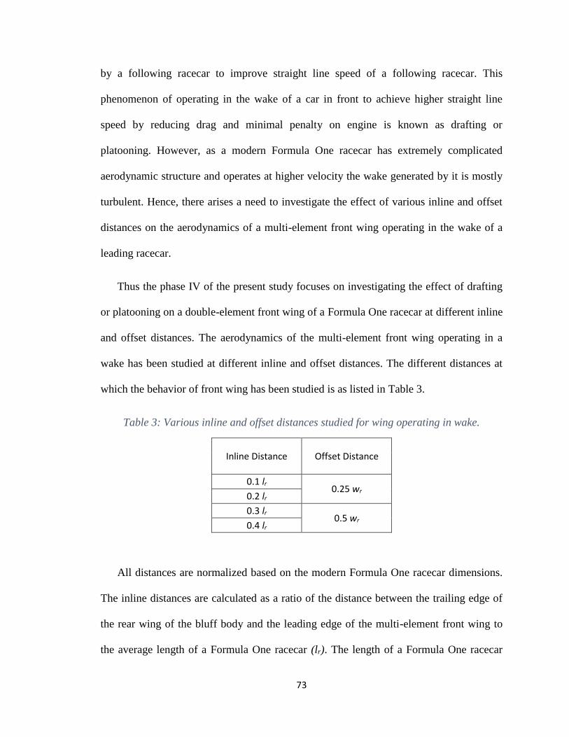
73
by a following racecar to improve straight line speed of a following racecar. This
phenomenon of operating in the wake of a car in front to achieve higher straight line
speed by reducing drag and minimal penalty on engine is known as drafting or
platooning. However, as a modern Formula One racecar has extremely complicated
aerodynamic structure and operates at higher velocity the wake generated by it is mostly
turbulent. Hence, there arises a need to investigate the effect of various inline and offset
distances on the aerodynamics of a multi-element front wing operating in the wake of a
leading racecar.
Thus the phase IV of the present study focuses on investigating the effect of drafting
or platooning on a double-element front wing of a Formula One racecar at different inline
and offset distances. The aerodynamics of the multi-element front wing operating in a
wake has been studied at different inline and offset distances. The different distances at
which the behavior of front wing has been studied is as listed in Table 3.
Table 3: Various inline and offset distances studied for wing operating in wake.
Inline Distance Offset Distance
0.1 lr 0.25 wr
0.2 lr
0.3 lr 0.5 wr
0.4 lr
All distances are normalized based on the modern Formula One racecar dimensions.
The inline distances are calculated as a ratio of the distance between the trailing edge of
the rear wing of the bluff body and the leading edge of the multi-element front wing to
the average length of a Formula One racecar (lr). The length of a Formula One racecar
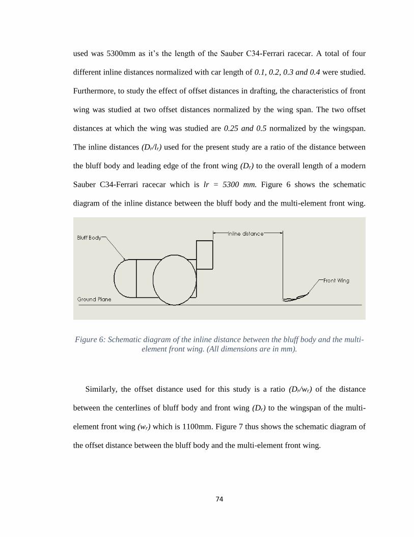
74
used was 5300mm as it’s the length of the Sauber C34-Ferrari racecar. A total of four
different inline distances normalized with car length of 0.1, 0.2, 0.3 and 0.4 were studied.
Furthermore, to study the effect of offset distances in drafting, the characteristics of front
wing was studied at two offset distances normalized by the wing span. The two offset
distances at which the wing was studied are 0.25 and 0.5 normalized by the wingspan.
The inline distances (Dr/lr) used for the present study are a ratio of the distance between
the bluff body and leading edge of the front wing (Dr) to the overall length of a modern
Sauber C34-Ferrari racecar which is lr = 5300 mm. Figure 6 shows the schematic
diagram of the inline distance between the bluff body and the multi-element front wing.
Figure 6: Schematic diagram of the inline distance between the bluff body and the multi-
element front wing. (All dimensions are in mm).
Similarly, the offset distance used for this study is a ratio (Dr/wr) of the distance
between the centerlines of bluff body and front wing (Dr) to the wingspan of the multi-
element front wing (wr) which is 1100mm. Figure 7 thus shows the schematic diagram of
the offset distance between the bluff body and the multi-element front wing.

75
Figure 7: Schematic diagram of the offset distance between the bluff body and the multi-
element front wing.
3.5. Wing model
For the current study, the front wing used is be a double-element front wing used in a
typical modern Formula One racecar. The airfoil used for this study is a highly cambered
double-element Formula One front wing consisting of two elements in a single slotted
flap configuration. The main element and the flap are a modified NASA GA (W) profile
of type LS (1)-0413 profile both possessing a finite trailing edge of 1.56mm and 0.95mm
respectively. A detailed listing of the co-ordinates can be found in Table 4 in appendix.
Both the elements are inverted to have suction surfaces closest to the ground. The main
element (cm) and flap (cf) has a chord of 223.4mm and 165.7mm respectively. For ease of
calculations, the total chord of 380mm is used for all calculations. Furthermore, for a

76
reference angle of attack (αo) of 00 for the wing, the true angle of attack for main element
(αm) and for flap (αf) will be of +3.60 and +15.50 respectively. Zerihan and Zhang
conducted the optimization of flap location for the said front wing and came up with
optimum values for flap gap (δg) and overlap (δo). These values are 0.024c and 0.032c
which corresponds to 9mm and 12mm for the overlap and gap respectively. In addition,
the wing has a span of 1100mm and an aspect ratio of AR = 2.89. A detailed listing of the
co-ordinates can be found in Table 4 in appendix. The schematic diagram of the front
wing used for the present study is shown in Figure 8 and 9.
Figure 8: Schematic of the double-element front wing used in the present study.
Figure 9: Schematic of the double-element front wing used in the present study with
angle of attack.

77
The described wing model is developed in SolidWorks 2016 and is as shown in
Figure 10 for the described parameters.
Figure 10: SolidWorks model of the wing
3.6. Bluff body
To study the aerodynamics of a multi-element front wing operating in the wake of a
racecar, a scaled model of bluff body is used which replicates the wake of a modern
Formula One racecar. The same multi-element front wing used in previous phases was
used in this phase to study the effect of drafting. In his study Wilson [27] showed that the
generic wake of a racecar can be represented with the help of bluff body such as one
shown in Figure 12. In a similar study conducted by Simon, it was found that a
significant drag reduction was observed when a single element front wing operated in the
wake of a racecar in front. In his study Simon made use of a similar scaled model which
was used by Wilson in his study of a front wing. In the present study a similar bluff body
has been created to study of drafting on the multi-element front wing. However, there are
some modifications made to the bluff body especially in the rear end to suit the present
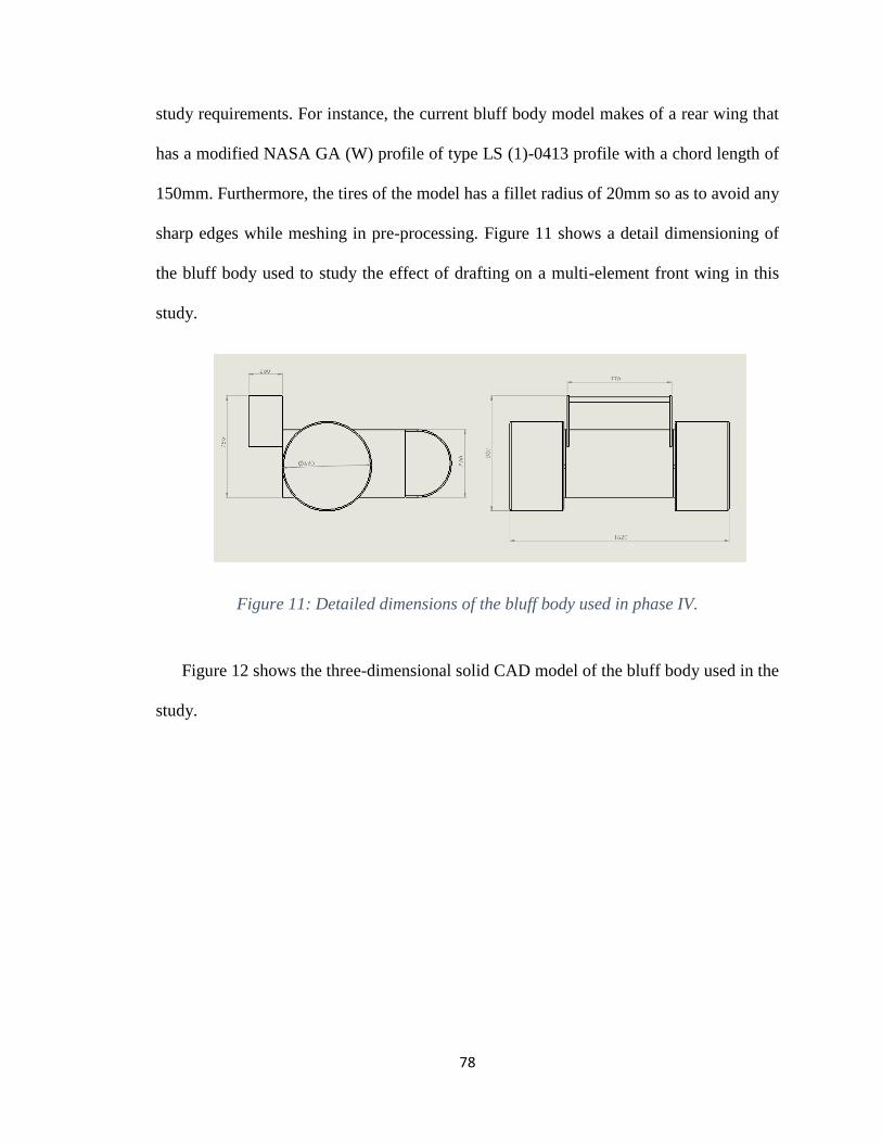
78
study requirements. For instance, the current bluff body model makes of a rear wing that
has a modified NASA GA (W) profile of type LS (1)-0413 profile with a chord length of
150mm. Furthermore, the tires of the model has a fillet radius of 20mm so as to avoid any
sharp edges while meshing in pre-processing. Figure 11 shows a detail dimensioning of
the bluff body used to study the effect of drafting on a multi-element front wing in this
study.
Figure 11: Detailed dimensions of the bluff body used in phase IV.
Figure 12 shows the three-dimensional solid CAD model of the bluff body used in the
study.

79
Figure 12: A solid model of the bluff body.

80
4. Methodology
4.1. Computational analysis
The study aims to achieve the said objectives by performing a computational analysis
using computational package STAR CCM+ developed by CD Adapco. STAR CCM+
solves the three-dimensional Reynolds-averaged Navier-Stokes equations (RANS) to
model the flow-field. These equations are based off the fundamental physics equations
for conservation of mass, momentum, and energy. The continuity equations model the
mass flux across a control volume also known as cell to ensure mass, momentum and
energy is conserved. The computational package mentioned solves these governing
equations with the help of differential approach as mentioned in the equation below
(Versteeg and Malalasekera 2007).
𝜕𝜌
𝜕𝑡+ 𝛻. (𝜌𝑢) = 𝟎 6
Differential approach is used by most computational packages as it is suitable for
performing detailed computational analysis such as investigating flow structures and
separation of boundary layers. By using the said differential approach, the governing
equations model the mass flux across a control volume or cell as shown below in Figure
13.

81
Figure 13: Control volume used for deriving governing equations.
The shown control volume has a length of each of its side along x, y and z
direction as δx, δy and δz respectively. Therefore, the volume of the cell above is given
by δxδyδz. Also, the origin for the shown control volume is such that its center is a point
with co-ordinates (x,y,z). Furthermore, the velocity component at the center of cell in x, y
and z direction is u, v and w respectively.
Now, using the control volume as shown in Figure 13 with the said parameters the
governing equation for mass, momentum and energy are derived and solved for a control
volume using differential approach. The mass flow rate in and out of a control volume
can be visualized as shown in Figure 14.

82
Figure 14: Mass fluxes rate over a control volume.
Thus, by using this control volume the equation for conservation of mass is
derived as shown below:
𝜕𝜌
𝜕𝑡+
𝜕(𝜌𝑢)
𝜕𝑥+
𝜕(𝜌𝑣)
𝜕𝑦+
𝜕(𝜌𝑤)
𝜕𝑧= 0 7
In equation 7 the first term represents the time rate of change in density for the cell.
However, for a steady state the 𝜕
𝜕𝑡= 0. Similarly, for an incompressible flow, the
𝜕𝜌
𝜕𝑡= 0.
In addition, using the same approach, the equation for conservation of momentum is
derived and is as shown by equation 8, 9 and 10 as,
𝜕(𝜌𝑢)
𝜕𝑡+
𝜕(𝜌𝑢𝑢)
𝜕𝑥+
𝜕(𝜌𝑣𝑢)
𝜕𝑦+
𝜕(𝜌𝑤𝑢)
𝜕𝑧=
𝜕(−𝜌 + 𝜏𝑥𝑥)
𝜕𝑥+
𝜕(𝜏𝑦𝑥)
𝜕𝑦+
𝜕(𝜏𝑧𝑥)
𝜕𝑧+ 𝑆𝑥 8
𝜕(𝜌𝑣)
𝜕𝑡+
𝜕(𝜌𝑢𝑣)
𝜕𝑥+
𝜕(𝜌𝑣𝑣)
𝜕𝑦+
𝜕(𝜌𝑤𝑣)
𝜕𝑧=
𝜕(𝜏𝑥𝑦)
𝜕𝑦+
𝜕(−𝜌 + 𝜏𝑦𝑦)
𝜕𝑥+
𝜕(𝜏𝑧𝑦)
𝜕𝑧+ 𝑆𝑦 9

83
𝜕(𝜌𝑤)
𝜕𝑡+
𝜕(𝜌𝑢𝑤)
𝜕𝑥+
𝜕(𝜌𝑣𝑤)
𝜕𝑦+
𝜕(𝜌𝑤𝑤)
𝜕𝑧=
𝜕(𝜏𝑥𝑧)
𝜕𝑥+
𝜕(𝜏𝑦𝑧)
𝜕𝑦+
𝜕(−𝜌 + 𝜏𝑧𝑧)
𝜕𝑧+ 𝑆𝑧 10
The equations 8, 9 and 10 represent the governing equation for conservation of
momentum. In these three equations, the first term represents the inertia forces, second
term represents pressure forces, third viscous forces and the last term represent the body
forces such as gravity. The final governing equation is the equation of conservation of
energy and is derived similarly as for mass and momentum and is given as,
𝜌𝐷𝐸
𝐷𝑡= [
𝜕(𝑢(−𝜌 + 𝜏𝑥𝑥))
𝜕𝑥+
𝜕(𝑢𝜏𝑦𝑥)
𝜕𝑦+
𝜕(𝑢𝜏𝑧𝑥)
𝜕𝑧] + [
𝜕(𝑣𝜏𝑥𝑦)
𝜕𝑦+
𝜕(𝑣(−𝜌 + 𝜏𝑦𝑦))
𝜕𝑥+
𝜕(𝑣𝜏𝑧𝑦)
𝜕𝑧] +
[𝜕(𝑤𝜏𝑥𝑧)
𝜕𝑥+
𝜕(𝑤𝜏𝑦𝑧)
𝜕𝑦+
𝜕(𝑤(−𝜌 + 𝜏𝑧𝑧))
𝜕𝑧] − [
𝜕(𝑞𝑥)
𝜕𝑥+
𝜕(𝑞𝑦)
𝜕𝑦+
𝜕(𝑞𝑧)
𝜕𝑧] + 𝑆𝐸 11
The equation for conservation of energy shown by equation (10), exists in several
forms in terms of temperature, enthalpy, internal energy and kinetic energy. Also, the last
term 𝑆𝐸 represents the source. However, in a computational fluid dynamics model, the
flow is assumed to be incompressible, therefore there is no need to solve the energy
equation. Furthermore, STAR CCM+ makes use of the ‘SIMPLE’ pressure-based
segregated algorithm recommended for steady-state calculations to decouple pressure and
velocity terms.
From the governing equations above, it can be observed, there are further some
unknowns which are known as viscous stresses. These viscous stresses are related to the
velocity gradient in x, y and z direction. Hence, there arises a need to introduce a suitable
model for these stresses (Versteeg and Malalasekera 2007). Navier-Strokes equation used
by the computational software to solve the fluid volume are introduced for the viscous

84
stresses from these governing equations for mass, momentum and energy. As discussed,
the CFD model assumes the flow to be incompressible, thus, the Navier-Strokes equation
for the incompressible flow is given as,
𝜌 (𝜕𝑢
𝜕𝑡+ 𝑢
𝜕𝑢
𝜕𝑥+ 𝑣
𝜕𝑢
𝜕𝑦+ 𝑤
𝜕𝑢
𝜕𝑧) = −
𝜕𝑝
𝜕𝑥+ 𝜇 (
𝜕2𝑢
𝜕𝑥2 +𝜕2𝑢
𝜕𝑦2 +𝜕2𝑢
𝜕𝑧2) + 𝜌𝑔𝑥 12
𝜌 (𝜕𝑣
𝜕𝑡+ 𝑢
𝜕𝑣
𝜕𝑥+ 𝑣
𝜕𝑣
𝜕𝑦+ 𝑤
𝜕𝑣
𝜕𝑧) = −
𝜕𝑝
𝜕𝑦+ 𝜇 (
𝜕2𝑣
𝜕𝑥2 +𝜕2𝑣
𝜕𝑦2 +𝜕2𝑣
𝜕𝑧2) + 𝜌𝑔𝑦 13
𝜌 (𝜕𝑢
𝜕𝑡+ 𝑢
𝜕𝑤
𝜕𝑥+ 𝑣
𝜕𝑤
𝜕𝑦+ 𝑤
𝜕𝑤
𝜕𝑧) = −
𝜕𝑝
𝜕𝑧+ 𝜇 (
𝜕2𝑤
𝜕𝑥2 +𝜕2𝑤
𝜕𝑦2 +𝜕2𝑤
𝜕𝑧2 ) + 𝜌𝑔𝑧 14
4.2. Flow conditions
The study is focused to represent the real racing conditions as much as possible.
Considering this, a three-dimensional steady state turbulent flow is considered for the
study. All the simulations will be performed with a freestream velocity of 30m/s
corresponding to a Reynolds number of 7.86 x 10⁵ based on chord length. The speed of
30m/s is chosen as it corresponds to the cornering speeds in Formula One. For the study,
as the wing operates at high speeds and the flow is incompressible, a segregated three-
dimensional flow is selected to solve for three-dimensional RANS equations along with
Gauss-Seidel relaxation scheme.
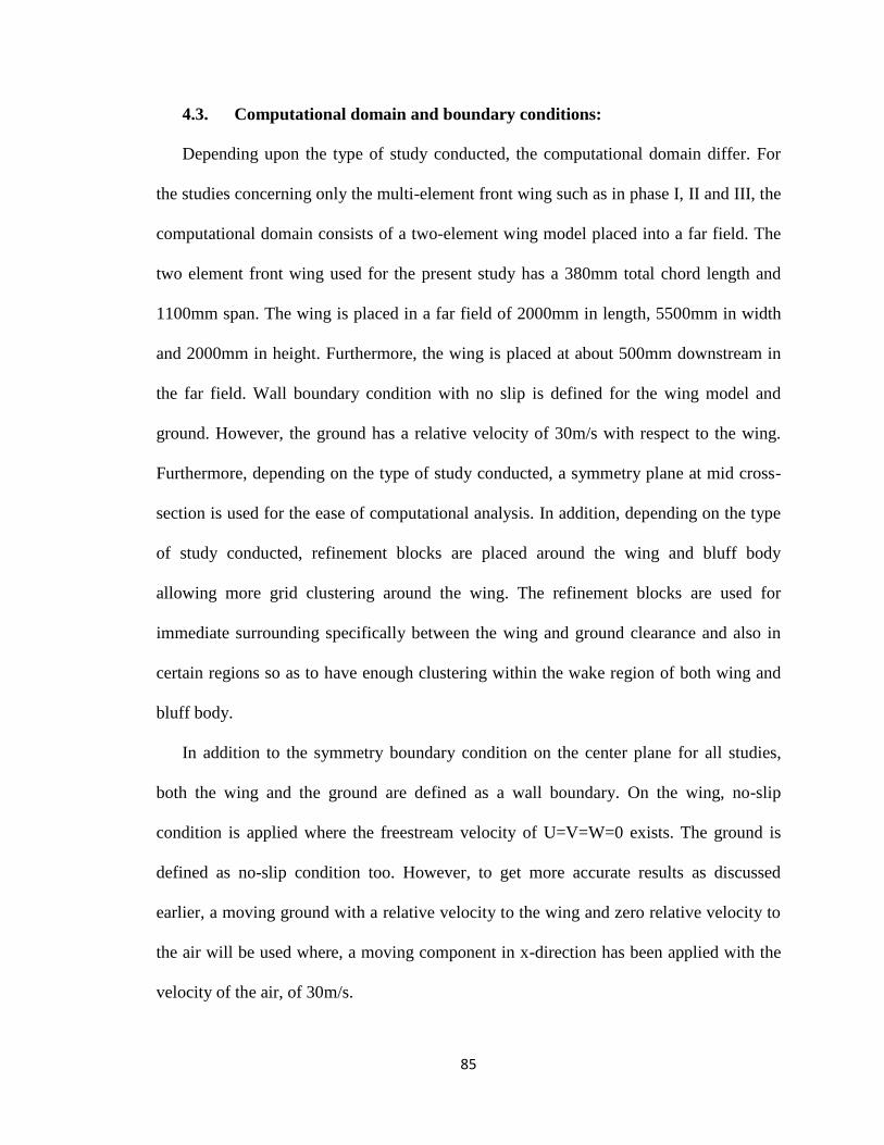
85
4.3. Computational domain and boundary conditions:
Depending upon the type of study conducted, the computational domain differ. For
the studies concerning only the multi-element front wing such as in phase I, II and III, the
computational domain consists of a two-element wing model placed into a far field. The
two element front wing used for the present study has a 380mm total chord length and
1100mm span. The wing is placed in a far field of 2000mm in length, 5500mm in width
and 2000mm in height. Furthermore, the wing is placed at about 500mm downstream in
the far field. Wall boundary condition with no slip is defined for the wing model and
ground. However, the ground has a relative velocity of 30m/s with respect to the wing.
Furthermore, depending on the type of study conducted, a symmetry plane at mid cross-
section is used for the ease of computational analysis. In addition, depending on the type
of study conducted, refinement blocks are placed around the wing and bluff body
allowing more grid clustering around the wing. The refinement blocks are used for
immediate surrounding specifically between the wing and ground clearance and also in
certain regions so as to have enough clustering within the wake region of both wing and
bluff body.
In addition to the symmetry boundary condition on the center plane for all studies,
both the wing and the ground are defined as a wall boundary. On the wing, no-slip
condition is applied where the freestream velocity of U=V=W=0 exists. The ground is
defined as no-slip condition too. However, to get more accurate results as discussed
earlier, a moving ground with a relative velocity to the wing and zero relative velocity to
the air will be used where, a moving component in x-direction has been applied with the
velocity of the air, of 30m/s.

86
Figure 15: The three-dimensional computational domain.

87
5. Phase I: Predictability of different turbulence and meshing models
In this phase of the current study, the predictive capability of the standard k- ω Shear
Stress Transport (SST) and the one equation Spalart-Allmarus turbulence model to
predict the three-dimensional flow over a multi-element front wing in ground effect is
determined. Also, the applicability of the structured trimmer and unstructured polyhedral
meshing models for a three-dimensional multi-element front wing is investigated in this
phase. To determine the accuracy of the said turbulence and meshing models, the
aerodynamic characteristics of a multi-element front wing is studied for a total of three
ground clearances of 0.224c, 0.09c and 0.05c at a reference velocity of 30m/s.
Furthermore, a paper [38] has been published for the study conducted in phase I in the
International Journal of Engineering Science and Innovative Technologies (IJESIT).
5.1. Geometric model
5.1.1. Wing model
The wing model used in this phase of current study is the same before mentioned
highly cambered double-element Formula One front wing consisting of two elements in a
single slotted flap configuration. The main element and the flap are a modified NASA
GA (W) profile of type LS (1)-0413 profile both possessing a finite trailing edge of
1.56mm and 0.95mm respectively. An in depth details regarding the wing model used in
the study is mentioned in the present study section.

88
5.2. Meshing model
In the present study, the applicability of two meshing models for a three-dimensional
multi element front wing is investigated. The two meshing models used are, an
unstructured polyhedral and a structured trimmer mesh models. For both the models, a
thin prism layer mesher is used along with a surface remesher and surface wrapper to get
more refined mesh. In addition, to effectively determine the applicability of both the
models, the reference values for both models are kept similar.
Once the appropriate model is selected, a refinement block around the multi-element
front wing is used to capture the region between the wing and ground plane and in the
wake of the wing.
5.3. Physics model
5.3.1. Computational domain and boundary conditions
The computational domain consists of the wing model placed in a far field of length
2000mm, width 5500mm and height of 1750mm. The wing is placed about 500mm
downstream in the far field. For boundary conditions, the wing and the ground is defined
as a wall boundary with no-slip condition. The wing is applied with a no slip condition
where U=V=W=0 exists. Furthermore, since a moving ground simulation is used, the
ground moves with a relative velocity of 30m/s in x-direction to the air. Figure 16 shows
the computational domain along with the wing model used in this phase of present study.

89
Figure 16: Computational domain used along with the wing model.
5.3.2. Turbulence model
As discussed earlier, selecting an adequate turbulence model is crucial as it
significantly affects the results. A proper turbulence model will predict the flow
accurately and thus yielding more correct results for lift and drag. Most of the CFD
software make use of RANS turbulence model to predicting turbulent flow. The
Reynolds Averaged Navier-Strokes equation is given as,
�̅�𝜕𝑢
𝜕𝑥+ �̅�
𝜕𝑢
𝜕𝑦+ �̅�
𝜕𝑢
𝜕𝑧=
1
𝑟
𝑑𝑝
𝑑𝑥+ 𝑣 (
𝜕2�̅�
𝜕𝑥2 +𝜕2𝑢
𝜕𝑦2 +𝜕2𝑢
𝜕𝑧2) − (𝜕𝑢′2̅̅ ̅̅ ̅
𝜕𝑥+
𝜕𝑢′𝑣′̅̅ ̅̅ ̅̅
𝜕𝑦+
𝜕𝑢′𝑤′̅̅ ̅̅ ̅̅ ̅
𝜕𝑧) 15
From the above equation, it can be seen, RANS solves for a total of 11 unknowns
of which 5 unknowns are related to the flow properties while the rest 6 are the knowns
for Reynolds stresses. These RANS turbulent models used by various CFD packages
solves the mean flow first and then adds the effects of turbulence. These RANS models
are specifically used to solve for the Reynolds stresses and thus are highly numerically
efficient as it eliminates the 6 unknowns related to Reynolds stresses. There exist several

90
turbulence models used by numerous CFD software which can be used to predict the
turbulent flow for the study. Through literature, it has been found that, all turbulence
models yield good results while predicting the flow over a front wing in freestream and
medium ground clearance (also known as force enhancement region). However, as for the
case of low ground clearance (force reversal region) not all turbulence models are able to
predict the flow structure.
From literature review, it is observed that the standard k- ω SST model and the
one equation Spalart-Allmarus turbulence model can accurately predict the flow for a
front wing in ground effect at low ride heights. Furthermore, it is observed that for
medium ground clearances or the force enhancement region, the standard k- ω SST model
predicts the flow more accurately. Whereas, the one equation Spalart-Allmarus
turbulence model can accurately predict the flow at lower ride heights or the force
reversal region.
The one equation Spalart-Allmarus turbulence model as the name suggests is a
one equation turbulence model developed by P. R. Spalart and S. R. Allmarus (Spalart
and Allmarus 1992). This model uses one equation to calculate the eddy viscosity. The
equation used to calculate eddy viscosity by one equation Spalart-Allmarus turbulence
model is,
𝜕�̃�
𝜕𝑡+ 𝑢𝑗
𝜕�̃�
𝜕𝑥𝑗= 𝐶𝑏1[1 − 𝑓𝑡2]�̃��̃� +
1
𝜎{𝛻. [(𝑣 + �̃�)𝛻�̃�] + 𝐶𝑏2|𝛻𝑣|2} −
[𝐶𝑤1𝑓𝑤 −𝐶𝑏1
𝑘2 𝑓𝑡2] (�̃�
𝑑)
2
+ 𝑓𝑡1 △ 𝑈2 16

91
where,
𝑣𝑡 = �̃�𝑓𝑣1, 𝑓𝑣1 =𝜒3
𝜒3+𝐶3𝑣1
, 𝜒 ≔�̃�
𝑣, �̃� = 𝑆 +
�̃�
𝜅2𝑑2 𝑓𝑣2 and 𝑓𝑡2 = 1 −𝜒
1+𝜒𝑓𝑣1
To solve for equation 12, the constants are modelled as shown below,
𝑓𝑡1 = 𝐶𝑡1𝑔𝑡𝑒𝑥𝑝 (−𝐶𝑡2𝜔𝑡
2
△𝑈2 [𝑑2 + 𝑔𝑡2𝑑𝑡
2]) 𝑓𝑡2 = 𝐶𝑡3𝑒𝑥𝑝(−𝐶𝑡4𝜒2)
𝑓𝜔 = 𝑔 [1+𝐶𝜔3
6
𝑔6+𝐶𝜔36]
1/6
, 𝑔 = 𝑟 + 𝐶𝜔2(𝑟6 − 𝑟), 𝑟 ≡�̃�
𝑆𝐾2𝑑2
𝛺𝑖𝑗 ≡1
2(
∂𝑢𝑖
∂𝑥𝑗−
∂𝑢𝑗
∂𝑥𝑖)
𝑆 =≡ √2𝛺𝑖𝑗𝛺𝑖𝑗
𝜎 = 2/3
𝐶𝑏1 = 0.1355
𝐶𝑏2 = 0.622
𝑘 = 0.41
𝐶𝑤1 = 𝐶𝑏1/𝑘2 + (1 + 𝐶𝑏2)/𝜎
𝐶𝑤2 = 0.3
𝐶𝑤3 = 2
𝐶𝑣1 = 7.1
𝐶𝑡1 = 1
𝐶𝑡2 = 2

92
𝐶𝑡3 = 1.1
𝐶𝑡4 = 2
As it makes use of one equation, the one equation Spalart-Allmarus turbulence
model is numerically efficient and can be used for simple geometries such as airfoils.
However, it can be used for predicting separated flows.
On the other hand, the standard k- ω Shear Stress Transport (SST) model makes
use of two equations to solve for the unknowns discussed (Menter 1993). It’s an
integration of the standard k- ε and k- ω turbulence models. In simple terms, the standard
k- ω SST model is used between these two models to overcome their shortcomings. For
instance, to predict flow near wall and for completely developed flow far from wall, it
makes use of k- ε model. Whereas, to predict flow for outer boundary layers and in
regions of separation, it makes use of k- ω model. Thus, the standard k- ω SST model is
highly efficient and is widely used for most of the studies. The two equations used by
standard k- ω SST model are as discussed below.
The eddy viscosity is calculated with the help of the equation below,
𝑣𝑇 =𝑎1𝑘
𝑚𝑎𝑥 (𝑎1𝜔,𝑆𝐹2) 16
Furthermore, the additional two governing equations used are as follows,
𝜕𝑘
𝜕𝑡+ 𝑈𝑗
𝜕𝑘
𝜕𝑥𝑗= 𝑃𝑘 − 𝛽 ∗ 𝑘𝜔 +
𝜕
𝜕𝑥𝑗[(𝑣 + 𝜎𝑘𝑣𝑇)
𝜕𝑘
𝜕𝑥𝑗] 17
𝜕𝜔
𝜕𝑡+ 𝑈𝑗
𝜕𝜔
𝜕𝑥𝑗= 𝛼𝑆2 − 𝛽𝜔2 +
𝜕
𝜕𝑥𝑗[(𝑣 + 𝜎𝑘𝑣𝑇)
𝜕𝜔
𝜕𝑥𝑗] + 2(1 − 𝐹1)𝜎𝜔2
1
𝜔
𝜕𝑘
𝜕𝑥𝑗
𝜕𝜔
𝜕𝑥𝑗 18
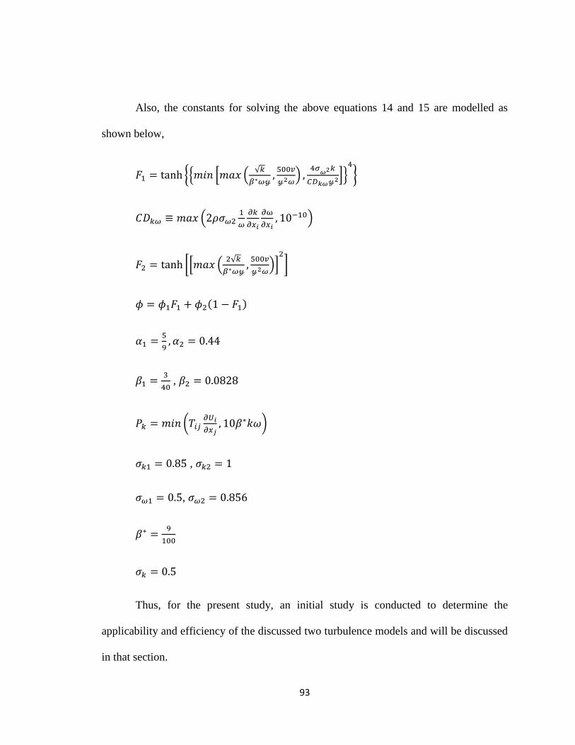
93
Also, the constants for solving the above equations 14 and 15 are modelled as
shown below,
𝐹1 = tanh {{𝑚𝑖𝑛 [𝑚𝑎𝑥 (√𝑘
𝛽∗𝜔𝓎,
500𝑣
𝓎2𝜔) ,
4𝜎𝜔2𝑘
𝐶𝐷𝑘𝜔𝓎2]}
4
}
𝐶𝐷𝑘𝜔 ≡ 𝑚𝑎𝑥 (2𝜌𝜎𝜔21
𝜔
∂𝑘
∂𝑥𝑖
∂ω
∂𝑥𝑖, 10−10)
𝐹2 = tanh [[𝑚𝑎𝑥 (2√𝑘
𝛽∗𝜔𝓎,
500𝑣
𝓎2𝜔)]
2
]
𝜙 = 𝜙1𝐹1 + 𝜙2(1 − 𝐹1)
𝛼1 =5
9, 𝛼2 = 0.44
𝛽1 =3
40 , 𝛽2 = 0.0828
𝑃𝑘 = 𝑚𝑖𝑛 (𝑇𝑖𝑗∂𝑈𝑖
∂𝑥𝑗, 10𝛽∗𝑘𝜔)
𝜎𝑘1 = 0.85 , 𝜎𝑘2 = 1
𝜎𝜔1 = 0.5, 𝜎𝜔2 = 0.856
𝛽∗ =9
100
𝜎𝑘 = 0.5
Thus, for the present study, an initial study is conducted to determine the
applicability and efficiency of the discussed two turbulence models and will be discussed
in that section.

94
5.3.3. Flow condition
To represent the real racing conditions as much as possible, a three-dimensional
steady state turbulent flow is considered for the study. The study is performed with a
freestream velocity of 30m/s corresponding to a Reynolds number of 7.86 x 10⁵ based on
chord length. The speed of 30m/s is chosen as it corresponds to the cornering speeds in
Formula One. For the study, as the wing operates at high speeds and the flow is
incompressible, a segregated three-dimensional flow is selected to solve for three-
dimensional RANS equations along with Gauss-Seidel relaxation scheme.
5.4. Results and discussion
5.4.1. Meshing
As mentioned earlier in methodology, two mesh models were used for the study
an unstructured polyhedral and a structured trimmer. To determine the applicability of
both the models, the reference values for both were kept similar. For both the models, a
base size of 0.1 m was used with prism layer meshing. A total of 15 prism layers were
used with a growth rate of 1.25. The surface curvature of 100 was used with a surface
growth rate of 1.1. The relative size of prism layer thickness of 20% corresponding to
0.02 m was used. A minimum surface thickness of 5% was used with a target of 100% to
keep the cell size as low as possible. For both models, about 400,000 cells were generated
and the volume mesh is as shown.

95
Figure 17: Volume mesh of a mid-plane using polyhedral (left) & trimmer (right) mesh
model.
It can be observed from Figure 17 that, for same configuration, the unstructured
polyhedral mesh model was able to capture a more refined mesh with a comparatively
steady growth rate. The cells along the far end of far field merge in a smoother manner in
polyhedral model thus giving a more refined mesh. The uniform growth rate for the
three-dimensional volume mesh can be clearly seen in Figure 18 which shows the volume
mesh of wing model using both models. This becomes more prominent when we observe
the mesh of the complete wing model as shown in Figure 18.

96
Figure 18: Mesh of a wing model using polyhedral (left) and trimmer (right) mesh model.
Thus, it was concluded that for the present study, the unstructured polyhedral
mesh model will be able to capture the wing model most efficiently. Hence, moving
forward for all the cases conducted in present study, the unstructured polyhedral meshing
model will be used. Also, to investigate the accuracy of two turbulence model a final
mesh of given wing model is created using a refinement block. The refinement block has
been defined so as to have a relative surface size of 3%. The final mesh for a ride height
of 0.224c with the use of a refinement block is shown in Figure 19.

97
Figure 19: Final mesh of mid-plane section with the refinement block.
5.4.2. Turbulence models
As discussed earlier, two turbulence models were studied for initial study, the
standard k- ω SST model and the one equation Spalart-Allmarus turbulence model. The
effect of these models on three different ride heights of 0.224c, 0.09c and 0.05c has been
analyzed and compared with the results from the experimental study conducted by
Zerihan and Zhang (Zhang and Zerihan, Aerodynamics of a Double-Element Wing in
Ground Effect 2003).
5.4.2.1. For medium ground clearance of 0.224c
For the multi-element front wing in medium ground clearances, both the
turbulence models are able to predict the flow with similar accuracy. As seen from
the residual plot of governing equation in Figure 20, both the models are able to

98
converge the governing equations properly with a relatively same residual error. By
observing the pressure and velocity contours for the wing model, it was seen that both
the turbulence models could accurately predict the flow at ground clearance of .224c.
Figure 20: Residual for both turbulence model at 0.224c
As mentioned, for the given ground clearance both the models are able to predict
the flow over the double-element front wing correctly. The highly-cambered double-
element single slotted front wing generates downforce with the help of Bernoulli’s

99
principle. The air flowing on the lower surface of the wing is forced downwards which
compresses it against the air below it and the ground. However, the air flowing over the
upper surface is expanded. Due to the compression, the air flowing on lower surface
flows at a higher velocity whereas, the air on upper surface flows at lower velocity due to
expansion. Now due to Bernoulli’s principle, the air flowing at higher velocity
experiences lower pressure than the air flowing on lower region. This pressure difference
between the upper and lower surfaces creates a force in downward direction, which is
known as downforce.
By analyzing the velocity and pressure distribution plots both the turbulence
models are able to predict this phenomenon accurately at ground clearance of 0.224c.
Figure 21 and Figure 22 show the velocity and pressure distribution plots using the one
equation Spalart-Allmarus and the standard k- ω Shear Stress Transport (SST) turbulence
models.

100
Figure 21: Velocity contour for mid-span plane using k- ω SST
Figure 22: Velocity contour for mid-span plane using Spalart-Allmarus

101
From the velocity vector distribution plots, the accelerated flow below the lower
surface can be clearly seen. The air flows at an accelerated speed of about 100% than the
freestream flow.
Furthermore, both the turbulence models are able to show the formation of
separation of boundary layer at the trailing edge. The pressure distribution plot for the
two models show this phenomenon clearly in Figure 23 and 24.
.
Figure 23: Pressure contour for mid-span plane using k- ω SST

102
Figure 24: Pressure contour for mid-span plane using Spalart-Allmarus
In order to measure the negative lift or downforce generated by the wing at this
ground clearance for both models, the lift coefficient (CL) is calculated and compared
with an existing study [20]. Both the turbulence models accurately predicted the value of
lift coefficient at the ground clearance of 0.224c.
5.4.2.2. For low ground clearance of 0.09c
As the ground clearance is lowered, the air flow between the wing and ground is
accelerated further thus, generating more downforce. By lowering the ground clearance
from 0.224c to 0.09c, the velocity of air on the lower surface of wing increased by 18.8%
causing a reduction in pressure. As a result of this, the lift coefficient is increased by
about 36%. Hence, indicating that the downforce indeed behaves as a function of ground

103
clearance. The air below the lower surface gets accelerated by about 172% than the
freestream air. The velocity distribution plots clearly show the further accelerated air in
Figure 25 and Figure 26 using both turbulence models. Also, by observing the pressure
distribution contours in Figure 27 and Figure 28, the separation of boundary layers at the
trailing edge appears to increase as the ground clearance is reduced.
Figure 25: Velocity contour for mid-span plane using k- ω SST

104
Figure 26: Velocity contour for mid-span plane using Spalart-Allmarus
Figure 27: Pressure contour for mid-span plane using k- ω SST

105
Figure 28: Pressure contour for mid-span plane using Spalart-Allmarus
By observing the velocity and pressure contours for both the turbulence models, it
is found that the one equation Spalart-Allmarus model shows a higher accelerated flow
than the standard k- ω SST model thus, also relating to a lower suction pressure.
Furthermore, by comparing the values for lift coefficient for the both the turbulence
models, it appears that the standard k- ω Shear Stress Transport (SST) turbulence model
is more accurate than the one equation Spalart-Allmarus. The value of lift coefficient
using standard k- ω SST turbulence model is more accurate with 5.6% variation.
Whereas, the one equation Spalart-Allmarus predicts the lift coefficient with an 11.3%
variation.

106
5.4.2.3. For very low ground clearance of 0.05c
When the ground clearance is reduced further, the downforce generated by the wing
is reduced. Thus, indicating that for very low ground clearances, a downforce reduction
occurs due to the separation of boundary layers at the trailing edge for very low ground
clearances and there exists a maximum lift coefficient for a particular ground clearance.
The separation of boundary layer at the trailing edge occurs due to the boundary layer not
being able to withstand the adverse pressure gradient associated with highly accelerated
flow at small ride heights. The separation of boundary layer at the trailing edge can be
clearly seen by observing the velocity and pressure contours in Figure 29 to 32.
Figure 29: Velocity contour for mid-span plane using k- ω SST
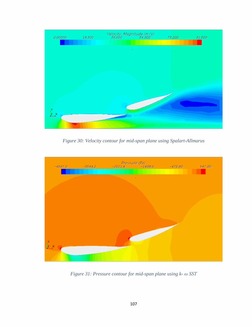
107
Figure 30: Velocity contour for mid-span plane using Spalart-Allmarus
Figure 31: Pressure contour for mid-span plane using k- ω SST

108
Figure 32: Pressure contour for mid-span plane using Spalart-Allmarus
Furthermore, for this very low ground clearance, the standard k- ω SST turbulence
model is able to predict the lift coefficient more accurately than the one equation Spalart-
Allmarus. The value of lift coefficient at 0.05c for standard k- ω SST turbulence is more
accurate with a 5.28% variation when compared to the 20.94% variation for the one
equation Spalart-Allmarus.
5.4.3. Accuracy in predicting the coefficient of lift
As mentioned earlier, the accuracy of the two turbulence model was determined by
comparing the results from the experimental study in [20]. Thus, the values of coefficient
of lift (CL) predicted by both the turbulence models were compared to the experimental
values from [20]. The values are plotted and the accuracy of both the turbulence models
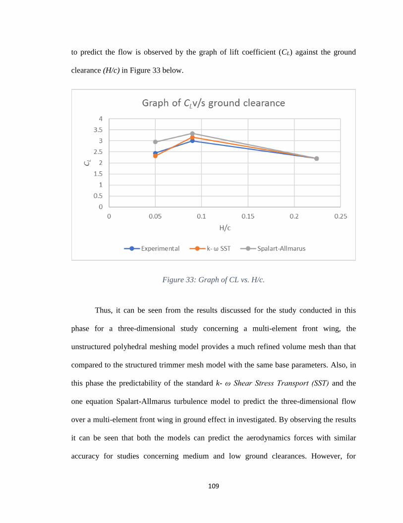
109
to predict the flow is observed by the graph of lift coefficient (CL) against the ground
clearance (H/c) in Figure 33 below.
Figure 33: Graph of CL vs. H/c.
Thus, it can be seen from the results discussed for the study conducted in this
phase for a three-dimensional study concerning a multi-element front wing, the
unstructured polyhedral meshing model provides a much refined volume mesh than that
compared to the structured trimmer mesh model with the same base parameters. Also, in
this phase the predictability of the standard k- ω Shear Stress Transport (SST) and the
one equation Spalart-Allmarus turbulence model to predict the three-dimensional flow
over a multi-element front wing in ground effect in investigated. By observing the results
it can be seen that both the models can predict the aerodynamics forces with similar
accuracy for studies concerning medium and low ground clearances. However, for

110
predicting the flow at very low ground clearances or for the downforce reduction region,
the standard k- ω Shear Stress Transport (SST) appears to be more accurate than the one
equation Spalart-Allmarus turbulence model.

111
6. Phase II: Wing in free stream
In this phase of current study as mentioned earlier, the described double element front
wing is studied in free stream to understand the aerodynamics of an inverted airfoil
operating as a racecar wing to generate negative lift otherwise known as downforce. The
three-dimensional free stream study is conducted at a reference velocity of 30m/s which
corresponds to the cornering speeds of modern Formula One racecars. Also, the study in
free stream will serve as a baseline case for further studies performed in the present
study.
6.1. Geometric model
6.1.1. Wing model
The wing profile used for the present study is a highly cambered single slotted double
element front wing used in a typical racecar. Both the main element and flap consist of a
modified NASA GA (W) profile of type LS (1) – 0413 possessing a finite trailing edge of
1.56mm for main element and of 0.95mm for the flap. In addition, the chord length of
main element and flap is 223.4mm and 165.7mm respectively. The total chord length of
the wing used was 380mm and all parameters such as ground clearance were normalized
by it. For the angle of attack calculations, the overall angle of attack (αo) of 0 degree
corresponds to +3.6 degrees angle of attack for main element (αm) and a +15.5 degrees
angle of attack for flap (αf). It is the same wing model that has been used in the phase I of
present study.

112
6.2. Meshing model
By observing the results in phase I of the current study, the unstructured polyhedral
meshing model has been used with a thin prism layer extruder. Figure 34 shows the
meshing model used for this phase of study.
Figure 34: Meshing model used for free stream case.
The model selected has a reference base size of 0.1 m with a minimum surface size
of 25% and a target size of 100% in reference to base size so as to generate a refined
mesh for this phase. Also, to allow more refinement a minimum surface size of 3% and a
target size of 5% is used for the main-element and flap along with a 10% prism layer
thickness all of which are relative to the base size of 0.1 m. Furthermore, a refinement
block was used to capture the wake of the wing. Figure 35 shows the refinement block
used in this phase of study.

113
Figure 35: Multi-element front wing in the computational domain along with the
refinement block used for meshing.
The final volume mesh consists of approximately 10 million cells and the resulting
mesh at mid-span cross section is as shown in Figure 36.

114
Figure 36: Mid-span cross section view of volume mesh using polyhedral meshing model.
Figure 37: Volume mesh of the multi-element front wing showing the thin prism layer
mesher.
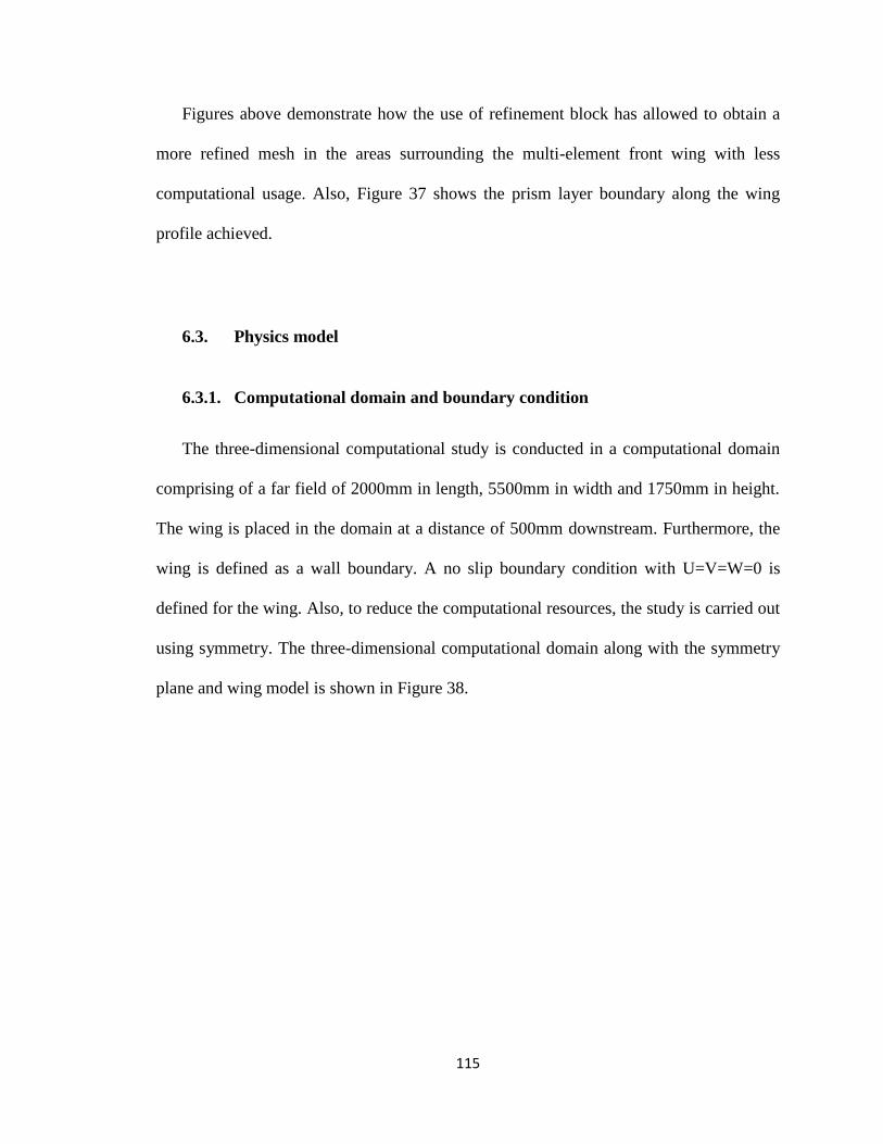
115
Figures above demonstrate how the use of refinement block has allowed to obtain a
more refined mesh in the areas surrounding the multi-element front wing with less
computational usage. Also, Figure 37 shows the prism layer boundary along the wing
profile achieved.
6.3. Physics model
6.3.1. Computational domain and boundary condition
The three-dimensional computational study is conducted in a computational domain
comprising of a far field of 2000mm in length, 5500mm in width and 1750mm in height.
The wing is placed in the domain at a distance of 500mm downstream. Furthermore, the
wing is defined as a wall boundary. A no slip boundary condition with U=V=W=0 is
defined for the wing. Also, to reduce the computational resources, the study is carried out
using symmetry. The three-dimensional computational domain along with the symmetry
plane and wing model is shown in Figure 38.

116
Figure 38: Computational domain along with the symmetry plane used for free stream
study.
6.3.2. Flow structure and turbulence model
For this phase a three-dimensional steady state turbulent flow is considered for the
study. The study is performed with a freestream velocity of 30m/s corresponding to a
Reynolds number of 7.86 x 10⁵ based on chord length. The speed of 30m/s is chosen as it
corresponds to the cornering speeds in Formula One. For the study, as the wing operates
at high speeds and the flow is incompressible, a segregated three-dimensional flow is
selected to solve for three-dimensional RANS equations along with Gauss-Seidel
relaxation scheme. Also, based on a study conducted in phase I, the standard k- ω Shear
Stress Transport (SST) turbulence model is used to predict the three-dimensional flow

117
characteristics of the wing. Also, for turbulence a turbulence viscosity ratio of 10 has
been selected. Figure 39 shows the physics model used for this phase of study.
Figure 39: Physics model used for the free stream case.
6.4. Results and discussion
The three dimensional free stream computational analysis was successfully conducted
at a reference velocity of 30m/s. The RANS equation model was successfully able to

118
predict the flow over a multi-element front wing in a free stream. A total of 1000
iterations are carried out and all the governing and turbulence equations are able to
converge properly within 0.01 residual error as shown in Figure 40.
Figure 40: Residual plot for free stream case.
Furthermore, by observing the lift and drag coefficient plots, it can also be seen
that the computational analysis has been able to converge properly as seen in Figure 41
and 42.
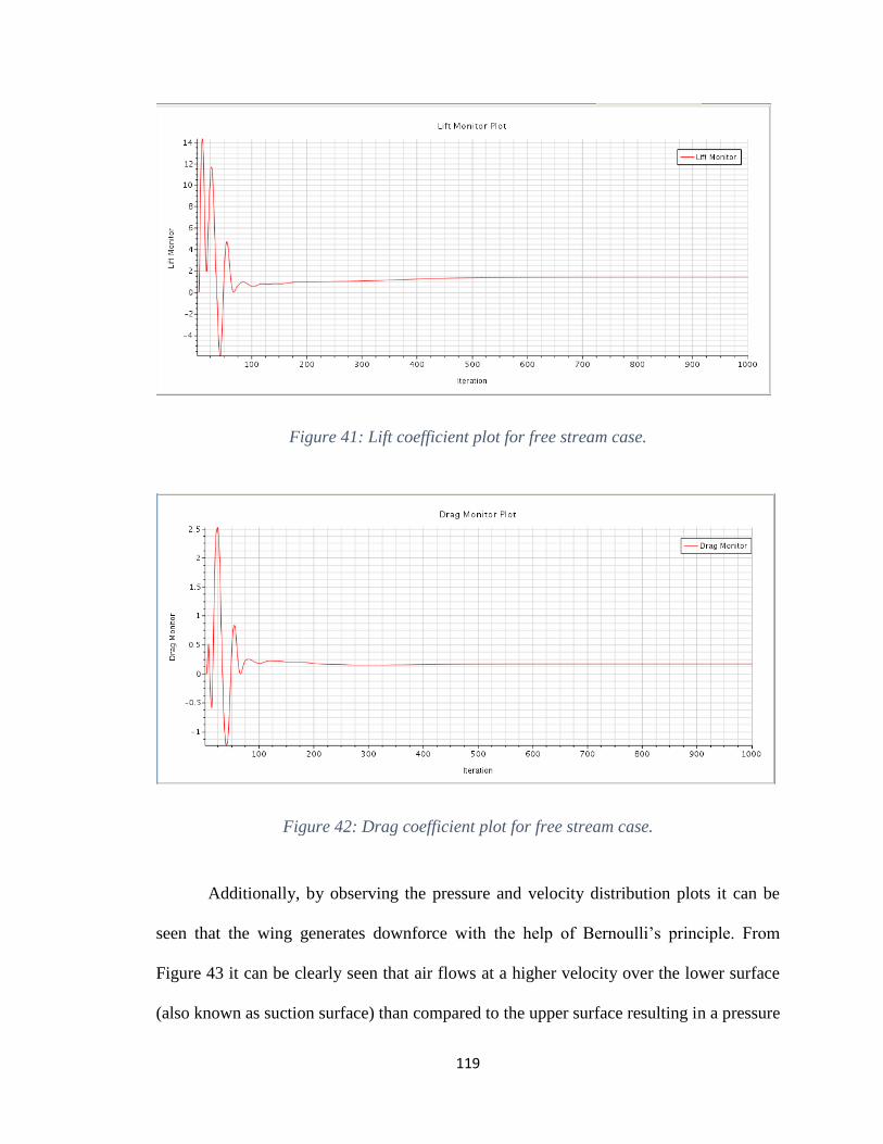
119
Figure 41: Lift coefficient plot for free stream case.
Figure 42: Drag coefficient plot for free stream case.
Additionally, by observing the pressure and velocity distribution plots it can be
seen that the wing generates downforce with the help of Bernoulli’s principle. From
Figure 43 it can be clearly seen that air flows at a higher velocity over the lower surface
(also known as suction surface) than compared to the upper surface resulting in a pressure
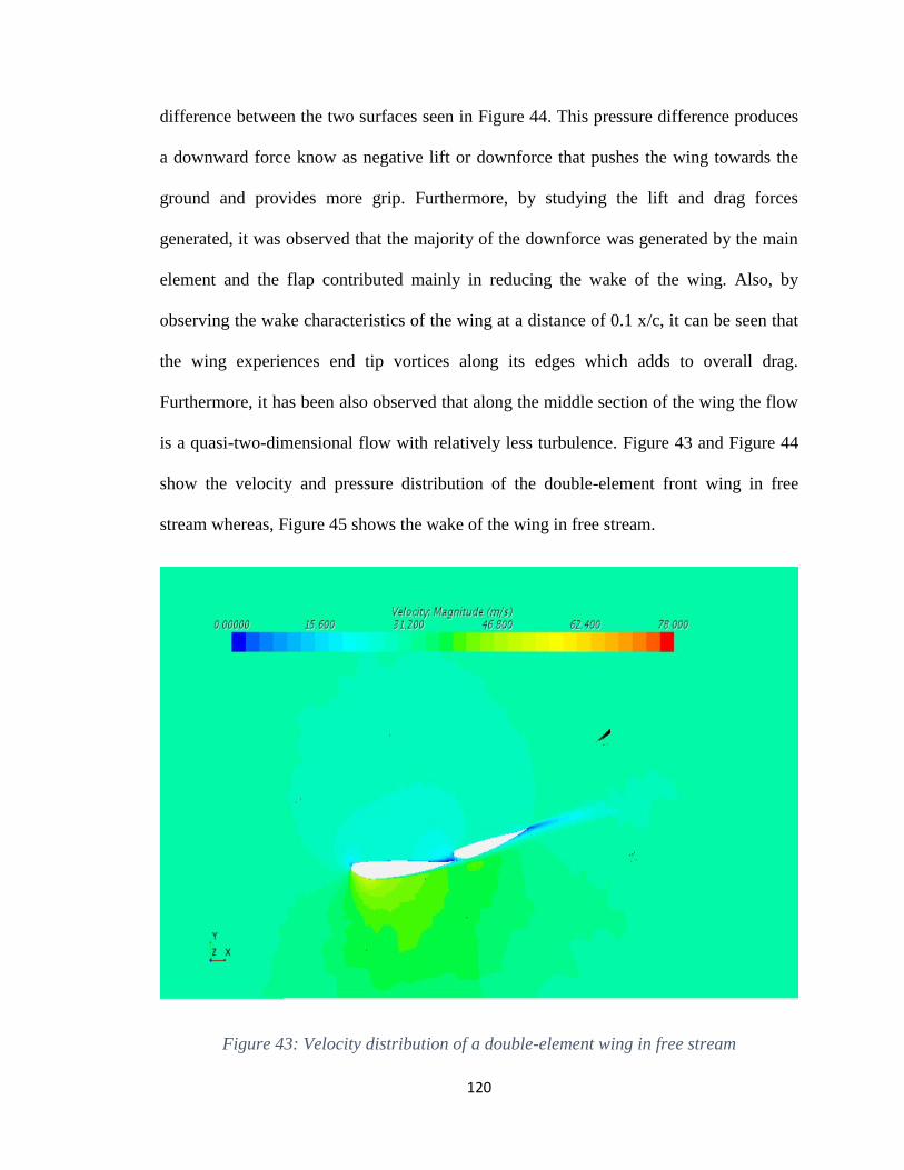
120
difference between the two surfaces seen in Figure 44. This pressure difference produces
a downward force know as negative lift or downforce that pushes the wing towards the
ground and provides more grip. Furthermore, by studying the lift and drag forces
generated, it was observed that the majority of the downforce was generated by the main
element and the flap contributed mainly in reducing the wake of the wing. Also, by
observing the wake characteristics of the wing at a distance of 0.1 x/c, it can be seen that
the wing experiences end tip vortices along its edges which adds to overall drag.
Furthermore, it has been also observed that along the middle section of the wing the flow
is a quasi-two-dimensional flow with relatively less turbulence. Figure 43 and Figure 44
show the velocity and pressure distribution of the double-element front wing in free
stream whereas, Figure 45 shows the wake of the wing in free stream.
Figure 43: Velocity distribution of a double-element wing in free stream

121
Figure 44: Pressure distribution of a double-element wing in free stream
Figure 45: Wake generated by the wing in free stream.

122
Moreover, the aerodynamic forces generated by the multi-element front wing in
free stream such as negative lift and drag has been calculated. For the described front
wing the coefficient of lift generated is about CL = 1.405 whereas, the drag coefficient is
about CD = 0.1674. In summary, the RANS turbulence model has been able to predict the
flow over the multi-element front in free stream properly. Also, the study demonstrates
how a racecar front wing is essentially an airfoil inverted when operating in free stream.
It also shows the formation of the end-tip vortices which results due the small aspect ratio
(AR) of the racecar wings and how it contributes to the drag generated. At last, the study
also provides a baseline for the studies concerning the ground effect, varying angle of
attacks and when wing is operated in the wake.

123
7. Phase III: Wing in ground effect and varying angle of attack
In this phase of present study, the two primary parameters affecting the aerodynamics
of a front wing, ground clearance and angle of attack has been investigated. The effect of
varying ground clearance and angle of attack on a multi-element front wing has been
determined in this phase. Hence, to study the effect of varying ground clearances, the
aerodynamic behavior of the multi-element front wing is studied at 10 different ride
heights of H/c=0.5, 0.3, 0.25, 0.224, 0.211, 0.15, 0.11, 0.09, 0.079 and 0.05 at a constant
angle of attack of 0 degree. In addition, the front wing is also studied for varying angle of
attack in ground effect. A total of 8 different angles are studied in this phase ranging from
0 degree to 13 degrees with an increment of 2 degrees. As mentioned earlier a reference
velocity of 30m/s was used for the three-dimensional analysis. Also, to get more realistic
results, a moving ground simulation has been used along with a three-dimensional flow.
7.1. Geometric model
7.1.1. Wing model
The wing model used for this phase is the same which has been used in the phase II of
this study where the flow over a multi-element front wing in free stream in investigated.
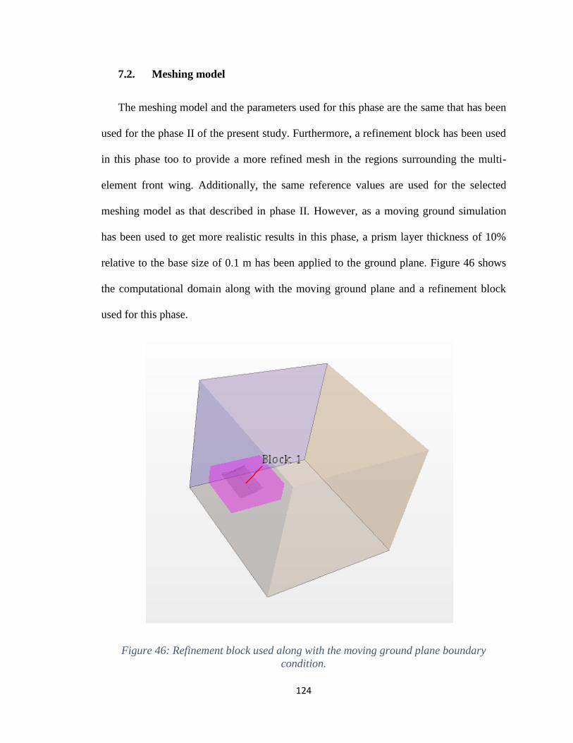
124
7.2. Meshing model
The meshing model and the parameters used for this phase are the same that has been
used for the phase II of the present study. Furthermore, a refinement block has been used
in this phase too to provide a more refined mesh in the regions surrounding the multi-
element front wing. Additionally, the same reference values are used for the selected
meshing model as that described in phase II. However, as a moving ground simulation
has been used to get more realistic results in this phase, a prism layer thickness of 10%
relative to the base size of 0.1 m has been applied to the ground plane. Figure 46 shows
the computational domain along with the moving ground plane and a refinement block
used for this phase.
Figure 46: Refinement block used along with the moving ground plane boundary
condition.

125
The resultant volume mesh obtained by using the described meshing model for
this phase has depending upon the ground clearance from about 1.5 million to 10 million
cells. The resultant volume mesh obtained at a ground clearance of H/c = 0.224 is as
shown in following figures.
Figure 47: Mid-span cross section view of volume mesh using polyhedral meshing model
at 0.224c.

126
Figure 48: Volume mesh obtained by using a refinement block and prism layer mesher at
0.224c.
Once again by observing Figure above it can be seen that more refinement is obtained
by using a refinement block with relatively less usage of computational resources. Also
observed from Figures of volume mesh it can be seen that more refinement has been
obtained in the regions between the wing and ground plane.
7.3. Physics model
7.3.1. Computational domain
The three-dimensional computational study is conducted in a computational domain
comprising of a far field of 2000mm in length, 5500mm in width and 1750mm in height.

127
The wing is placed in the domain at a distance of 500mm downstream. Furthermore, the
wing and ground are defined as a wall boundary. A no slip boundary condition with
U=V=W=0 is defined for the wing whereas to get more realistic results a moving ground
simulation was conducted with a reference velocity of 30m/s. Also, to reduce the
computational resources, all the cases were carried out using symmetry. The mid-span
cross-sectional plane has been defined as the symmetry plane for this phase. The three-
dimensional computational domain along with the symmetry plane and wing model is
shown in Figure 46.
7.3.2. Flow structure and turbulence model
The flow condition use in this phase is the same as that used in phase II of this study.
All the different cases of varying ground clearances and angle of attacks has been carried
out at a free stream velocity of 30m/s as it is the usual cornering speed of modern
Formula One racecars.
7.4. Results and discussion
7.4.1. Wing in ground effect
The effect of varying ground clearances on the aerodynamics of the multi-element
front wing has been investigated in this phase of study. The front wing has been studied
for a total of 10 different ground clearances. The ground clearance (H/c) has been
measured as a ratio of the perpendicular distance between the lowest point on suction
surface of wing and the ground plane (H) to the total chord length of the wing (c). The

128
various ground clearances at which the front wing has been studied are H/c = 0.5, 0.3,
0.25, 0.224, 0.211, 0.15, 0.11, 0.09, 0.079 and 0.05. Additionally, for all the 10 ground
clearances, the front wing has been kept at a constant angle of attack of 0 degree. For all
the cases, a RANS turbulence model has been used. Also, considering the results from
the study conducted in phase I, the standard k- ω SST turbulence model is used to predict
the turbulent flow over the multi-element front wing. The resultant flow structures and
aerodynamic forces generated are as discussed follows:
7.4.1.1. Flow structures
To study the effect of varying ground clearances, the flow characteristics of the
double-element wing has been investigated at 10 different ride heights of H/c=0.5, 0.3,
0.25, 0.224, 0.211, 0.15, 0.11, 0.09, 0.079 and 0.05 at a constant overall angle of attack of
0 degree and a moving ground simulation. As mentioned earlier a reference velocity of
30m/s was used for the three-dimensional analysis. After about 1000 iterations, the
aerodynamics of a multi-element front wing in ground effect has been successfully able
to predict by the RANS model. All the governing and continuity equations converged
properly within a residual error of 0.001. The following Figure 49 shows the residual plot
for a ground clearance of H/c = 0.224 whereas, Figure 50 to 51 show the velocity
distribution plots of the mentioned wing at ground clearance of 0.5H/c, 0.224H/c,
0.09H/c and 0.05H/c respectively.
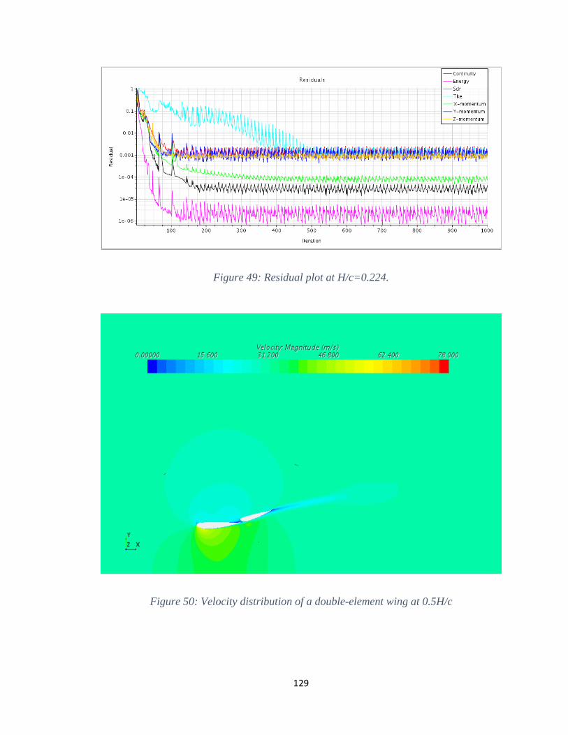
129
Figure 49: Residual plot at H/c=0.224.
Figure 50: Velocity distribution of a double-element wing at 0.5H/c

130
Figure 51: Velocity distribution of a double-element wing at 0.224H/c
Figure 52: Velocity distribution of a double-element wing at 0.09H/c

131
Figure 53: Velocity distribution of a double-element wing at 0.05H/c
By observing Figures above it can be clearly seen that the front wing behaves as an
inverted airfoil. However, it can also be observed from the velocity distribution plots that,
as the ground clearance decreases, the flow between the suction surface and ground is
accelerated further and it achieves higher values of velocity. This is a result of decreasing
ground clearance as the region between the front wing and ground plane having a nozzle
effect on the airflow. As the ground clearance reduces, the air is forced to flow in a
relatively smaller region resulting in a higher velocity airflow in the suction region.
Furthermore, according to the Bernoulli’s principle, this accelerated flow thus results in a
lower pressure values at the suction surface leading to a higher pressure difference
between two surfaces. This pressure difference can be clearly seen in the following
figures which show the pressure distribution of the wing at these ground clearances as
shown.

132
Figure 54: Pressure distribution of a double-element wing at 0.5H/c
Figure 55: Pressure distribution of a double-element wing at 0.224H/c

133
Figure 56: Pressure distribution of a double-element wing at 0.09H/c
Figure 57: Pressure distribution of a double-element wing at 0.05H/c

134
Thus by observing the velocity and pressure distribution plots it can be inferred that,
the decreasing ground clearance creates a nozzle effect where air flows at an accelerated
velocity with decreasing ride heights. By Bernoulli’s principle, this accelerated airflow
then leads to lower suction pressure value at the suction surface resulting in a higher
pressure difference. Moreover, this higher pressure difference between two surfaces
eventually results in a higher value of negative lift force (or downforce) being generated
by the wing. In addition, by observing the wake characteristics of wing at decreasing
ground clearances, it can be seen that the ground plane assists in eliminating the end tip
vortices. Following figures show the wake characteristics of wing at decreasing ground
clearances.
Figure 58: Wake characteristics of a double-element wing at 0.5H/c

135
Figure 59: Wake characteristics of a double-element wing at 0.224H/c
Figure 60: Wake characteristics of a double-element wing at 0.09H/c

136
Figure 61: Wake characteristics of a double-element wing at 0.05H/c
By observing the wake distribution plots, it can be seen that lowering the ground
clearance also helps in eliminating the end-tip vortices. As the wing is lowered, the
ground plane prohibits the formation of end-tip vortices and eventually reduces the
impact of induced drag on the front wing. Also, when compared to the free stream case,
these end-tip vortices appear to be having less impact and thus lower effect of induced
drag observed in finite wings as discussed.
7.4.1.2. Aerodynamic forces generated
The ultimate goal of using a multi-element front wing is to get maximum downforce
(negative lift) with less penalty on drag generated. Thus for the mentioned multi-element
front wing, a plot of coefficient of lift against the decreasing ground clearance has been

137
plotted and compared to that from the free stream case from phase II of current study.
Figure 62 and Figure 63 shows the graph of coefficient of lift and drag plotted against the
decreasing ground clearance respectively.
Figure 62: Graph of coefficient of lift vs. H/c.
0
0.5
1
1.5
2
2.5
0 0.1 0.2 0.3 0.4 0.5 0.6
Vs.
H/c
Lift coefficient vs. H/c
In ground effect
Free stream

138
Figure 63: Graph of coefficient of drag vs. H/c
It can be seen from the graphs that, the ground plane has a significant impact on
the aerodynamic forces generated by the multi-element front wing. When the front wing
is placed in a moving ground, the downforce generated increases significantly suggesting
a positive impact of ground plane in downforce generation. Additionally, as seen from
the wake distribution plots, the ground plane assists in eliminating the impact of induced
drag generated as a result of the end-tip vortices.
Moreover, it can also be observed from the graphs that as the ground clearance is
reduced, the ground plane has a positive impact on the downforce generated by the front
wing. In other words, downforce generated by the multi-element front wing behaves as a
function of ground clearance i.e. for every decrease in ground clearance, there is a
significant increase in downforce generated. Also, from the graph of drag coefficient, it
0
0.05
0.1
0.15
0.2
0.25
0.3
0 0.1 0.2 0.3 0.4 0.5 0.6
Co
effi
cien
t o
f d
rag
H/c
Coefficient of drag vs. H/c
In ground effect
Free stream

139
can be seen that there is a comparatively less increase in drag when the ground clearance
is lowered. This region where the front wing behaves as a function of ground clearance
from about H/c = 0.3 to 0.09 is also known as the region of downforce enhancement. As
seen from the velocity and pressure plots, the decreasing ground clearance causes a
nozzle effect, which results to a higher accelerated airflow over the suction surface of
front wing leading to a higher pressure difference and thus higher values of downforce.
The downforce generated reaches a maximum at about H/c = 0.09. However, any
decrease in ground clearance after that results in a reduction of downforce generated by
the front wing. This phenomenon is known as the downforce reduction phenomenon
which as seen from the graph is observed for very low ground clearances of H/c = 0.079
and 0.05. As observed from the velocity and pressure distribution plots, the reason for the
downforce reduction is due to the separation of boundary layers at the trailing edge of
wing. This separation of boundary layers is a result of boundary layers at trailing edge not
capable of withstanding the adverse pressure gradient associated with accelerated flow at
very low ground clearances. However, on the other hand, the drag generated by the front
wing has a linear behavior and it keeps on increasing with every decrease in ground
clearance.
7.4.2. Effect of varying angle of attacks in ground effect
In the present study, the effect of varying overall angle of attack with decreasing
ground clearance has also been investigated. The overall angle of attack has been varied
from 0 degree to 13 degrees with a simultaneous decrease in ground clearance from H/c

140
= 0.11 to 0.015. Furthermore, by studying the lift and drag forces generated the plot of
coefficient of lift and drag has been plotted against overall angle of attack and is as
shown in Figure 64 and Figure 65.
Figure 64: Graph of Coefficient of lift vs. varying angle of attack in ground effect.
0
0.5
1
1.5
2
2.5
0 2 4 6 8 10 12 14
Vs.
Angle of attack
Coefficient of lift vs. varying angle of attack in ground effect

141
Figure 65: Graph of Coefficient of drag vs. varying angle of attack in ground effect
It can be seen from the graph of lift coefficient above that there exist three regions. In
the first region there is an immediate increase in downforce generated as increasing angle
of attack increases camber and decreasing the ground clearance also facilitates in
enhancing downforce generated as there is no separation of boundary layers yet. For the
second region, for angle of attack from 1 degree to 9 degrees and corresponding ground
clearance from 0.1H/c to 0.044H/c, the downforce generated decreases. It can be stated
that the flow characteristics of the wing are affected strongly by the changes in ground
clearances than the changes in angle of attack. Thus, even though there is an increase in
overall angle of attack, the downforce generated decreases as the ground clearance
decreases below 0.1H/c. On the other hand, for higher values of angle of attacks the
camber of the front wing increases which eventually leads to an increase in downforce
0
0.1
0.2
0.3
0.4
0.5
0.6
0 2 4 6 8 10 12 14
Co
effi
cien
t o
f d
rag
Angle of attack
Coefficient of drag vs. varying angle of attack in ground effect

142
generated. This increase in downforce is indicated in the graph above where for A.O.A.
more than 9 degrees, the lift coefficient increases.
On contrary, the drag generated by the multi-element front wing increases in a linear
fashion as indicated by the graph of drag coefficient above. The airflow at the trailing
edge of the front wing separates for every increase in the angle of attack resulting in an
increase in drag force generated. This can be also seen from the velocity and pressure
distribution of wing at 1, 5, 9 and 13 degrees shown in following figures.
Figure 66: Velocity distribution of a double-element wing at 1 degree and 0.1H/c

143
Figure 67: Velocity distribution of a double-element wing at 5 degrees and 0.075H/c.
Figure 68: Velocity distribution of a double-element wing at 9 degrees and 0.044H/c

144
Figure 69: Velocity distribution of a double-element wing at 13 degrees and 0.015H/c
Figure 70: Pressure distribution of a double-element wing at 1 degree and 0.1H/c
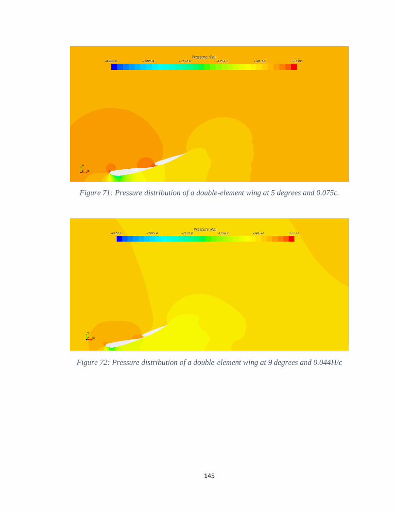
145
Figure 71: Pressure distribution of a double-element wing at 5 degrees and 0.075c.
Figure 72: Pressure distribution of a double-element wing at 9 degrees and 0.044H/c

146
Figure 73: Pressure distribution of a double-element wing at 13 degrees and 0.015H/c
Thus, by studying the double-element front wing in free stream, it has been
observed that the double-element front wing behaves as an inverted airfoil in free stream
generating downforce with the help of Bernoulli’s principle.
Also, when subjected to decreasing ground clearance, the wing exhibits two
distinct regions of downforce generation. A force enhancement region for medium
ground clearances where downforce behaves as a function of ground clearance and a
force reduction region for very low ground clearances where the downforce generated
reduces. It has also been observed that the separation of boundary layers is the reason for
the force reduction. Furthermore, the flow characteristics for increasing angle of attack
with simultaneous decrease in ground clearance indicate that ground plane has more
impact in determining the downforce generate for lower values of overall angle of attack.
However, for very low values of ground clearances and higher values of angle of attack,
the downforce generated increase as the angle of attack has a significantly more impact.
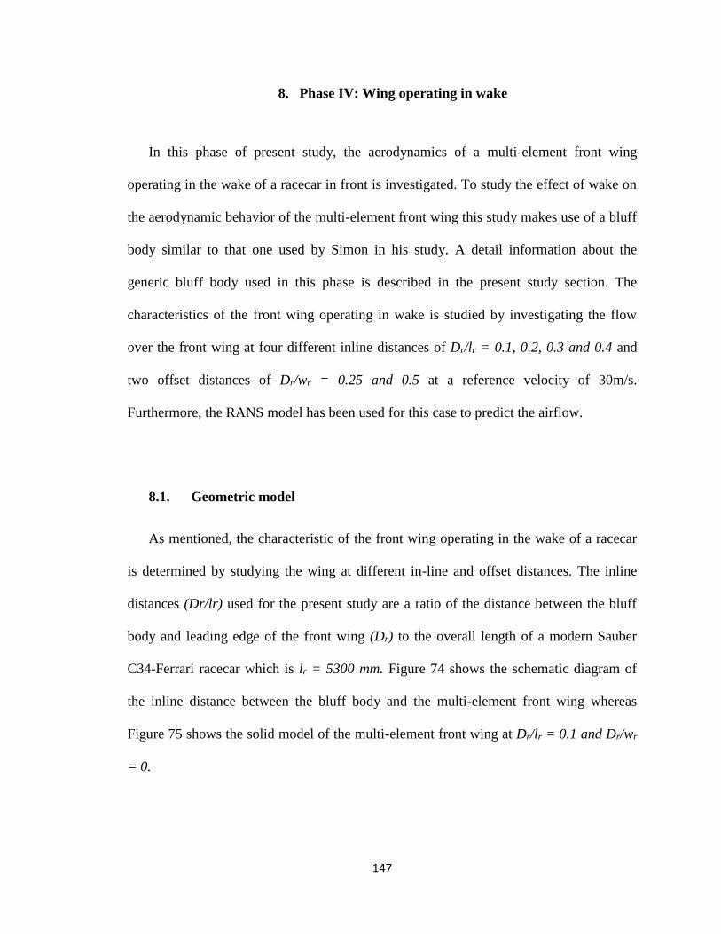
147
8. Phase IV: Wing operating in wake
In this phase of present study, the aerodynamics of a multi-element front wing
operating in the wake of a racecar in front is investigated. To study the effect of wake on
the aerodynamic behavior of the multi-element front wing this study makes use of a bluff
body similar to that one used by Simon in his study. A detail information about the
generic bluff body used in this phase is described in the present study section. The
characteristics of the front wing operating in wake is studied by investigating the flow
over the front wing at four different inline distances of Dr/lr = 0.1, 0.2, 0.3 and 0.4 and
two offset distances of Dr/wr = 0.25 and 0.5 at a reference velocity of 30m/s.
Furthermore, the RANS model has been used for this case to predict the airflow.
8.1. Geometric model
As mentioned, the characteristic of the front wing operating in the wake of a racecar
is determined by studying the wing at different in-line and offset distances. The inline
distances (Dr/lr) used for the present study are a ratio of the distance between the bluff
body and leading edge of the front wing (Dr) to the overall length of a modern Sauber
C34-Ferrari racecar which is lr = 5300 mm. Figure 74 shows the schematic diagram of
the inline distance between the bluff body and the multi-element front wing whereas
Figure 75 shows the solid model of the multi-element front wing at Dr/lr = 0.1 and Dr/wr
= 0.

148
Figure 74: Schematic diagram of the inline distance between the bluff body and the
multi-element front wing
Figure 75: Three-dimensional solid model of the wing operating in wake at Dr/lr=0.1
and Dr/wr=0
Similarly, the offset distance used for this study is a ratio (Dr/wr) of the distance
between the centerlines of bluff body and front wing (Dr) to the wingspan of the multi-
element front wing (w) which is 1100mm. Figure 76 thus shows the schematic diagram of
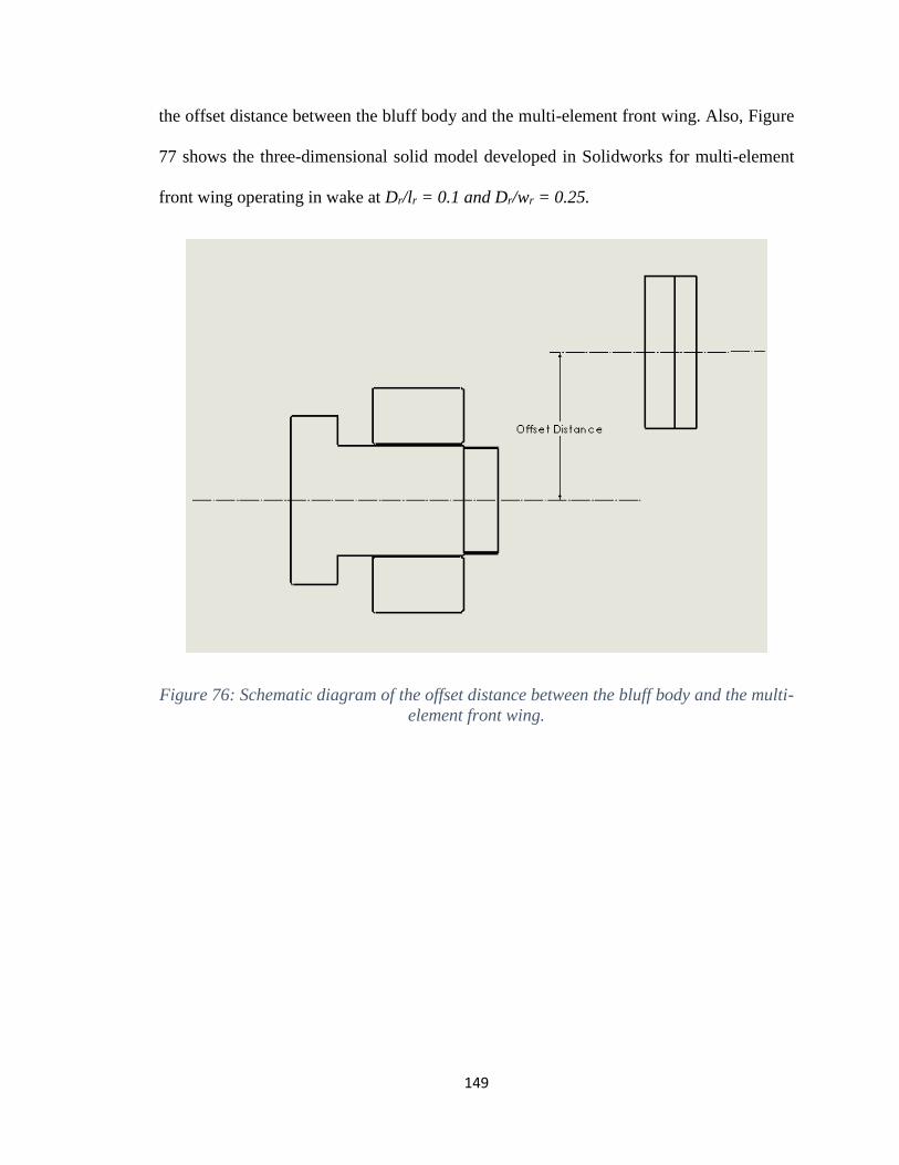
149
the offset distance between the bluff body and the multi-element front wing. Also, Figure
77 shows the three-dimensional solid model developed in Solidworks for multi-element
front wing operating in wake at Dr/lr = 0.1 and Dr/wr = 0.25.
Figure 76: Schematic diagram of the offset distance between the bluff body and the multi-
element front wing.

150
Figure 77: Three-dimensional solid model of the wing operating in wake at Dr/lr =0.1
and Dr/wr=0.25
The geometric model for this phase of the current study consists of a wing model and
bluff body which are as described follows:
8.1.1. Wing model
The wing model used for this phase is the same which has been used in the phase II of
this study where the flow over a multi-element front wing in free stream in investigated.
The multi-element front wing used in this phase of the study for all the various cases has
been used at constant ground clearance of 0.11c and a constant angle of attack of 1
degree as these parameters from the study conducted in phase III gave best values for
downforce and drag generated.

151
8.1.2. Bluff body
To represent the wake generated by a modern Formula One racecar, the present study
makes use of a generic bluff body which has been derived from the same bluff bodies
used by Wilson and Simon in their respective studies. An in-depth dimensioning and the
wing profile used by the bluff body in present study has been described in the present
study section.
8.2. Meshing model
To study the effect of multi-element front wing operating in wake, at first a baseline
case is studied. In this baseline case, the aerodynamics of only the bluff body used is
investigated to determine the wake generated by it. Once the wake generated by the bluff
body has been determined, the data can be used for conducting the studies for inline and
offset distances.
Thus, the meshing models differs for the study consisting of only the bluff body than
that for the different inline and offset distances between the bluff body and the front
wing. The basic meshing model for both type of studies remains the same as that of used
in phase II of present study as shown in Figure 34. However as shown in Figure 78, for
the study of bluff body, only one refinement block has been used to get more refinement
in the wake of the bluff body.

152
Figure 78: Computational domain along with the refinement block used for the bluff body
study.
Furthermore, for the study of bluff body, the minimum surface size of 5% and a
target surface size of 10% relative to the base size of 0.1 m has been used for the bluff
body. Also, a prism layer thickness of 10% relative to base size has been used for the
boundary layer thickness. The resultant generated volume mesh contains about 4.5
million cells and is as shown in Figure 79.

153
Figure 79: Volume mesh for the bluff body at symmetry plane
It can be clearly seen from Figure that more refinement is achieved in the wake of
the bluff body with the help of the one refinement block.
Similarly, the same meshing model is used for the study consisting the bluff body
and the front wing in different inline and offset distances arrangement. However, in these
studies, the model makes use of two refinement blocks as shown in Figure 80.

154
Figure 80: Computational domain along with the refinement blocks used for the
Dr/lr=0.2 and Dr/wr=0.
As shown in Figure, the two refinement blocks are used to capture more
refinement in the regions in between the bluff body and the front wing and in the wake of
the front wing. Additionally, the same minimum and target surface size used for the bluff
body study is used along with the same values used for the wing in phase II. Depending
upon the inline and offset distances used, the resultant volume mesh contains between 8
million to 11 million cells. The resultant volume mesh for the Dr/lr = 0.2 and Dr/wr = 0 is
as shown in Figure 81 which shows the impact of using two refinement blocks.

155
Figure 81: Volume mesh at mid-plane cross-section for Dr/lr=0.2 and Dr/wr=0/.
8.3. Physics model
8.3.1. Computational domain and boundary conditions
The computational domain for conducting the study of only the bluff body differs
from that of one in which the effect of different inline and offset distances are
investigated. The computational domain used for the study consisting of only the bluff
body has a computational domain of 7500mm in length, 2000mm in height and 4500mm
in width. The bluff body is placed at a distance of 1250mm downstream in the
computational domain. Also, the bluff body is defined as a wall boundary. A no slip
boundary condition with U=V=W=0 is defined for the bluff body whereas to get more
realistic results a moving ground simulation was conducted with a reference velocity of
30m/s. Additionally, to reduce the computational resources, the study is carried out using
symmetry at a mid-cross-sectional plane. The three-dimensional computational domain
along with the symmetry plane and wing model is shown in Figure 78. Similarly, for the
studies consisting the bluff body and front wing at different inline and offset distances,

156
the computational domain has been modified. Figure 80 shows the computational domain
used these types of studies where it has a depending upon the inline distances a length
from 8000mm to 11000mm and depending on the offset distances width from 4500mm to
5500mm.
Furthermore, for the different inline and offset distances studies, no symmetry has
been used. The bluff body, wing and ground are defined as a no slip wall boundary
condition defined as U=V=W=0. Whereas to get more realistic results a moving ground
simulation was conducted with a reference velocity of 30m/s.
8.3.2. Flow structure and turbulence model
The flow condition use in this phase is the same as that used in phase II of this study.
All the different cases of varying inline and offset distances has been carried out at a free
stream velocity of 30m/s as it is the usual cornering speed of modern Formula One
racecars.
8.4. Results and discussion
The computational study of a multi-element front wing operating in the wake of a
racecar has been successfully conducted by using RANS model to predict the three-
dimensional flow. The results obtained are as discussed:

157
8.4.1. Wake generated by the bluff body
At first a three-dimensional computational analysis of only the bluff body has been
conducted to study the wake generated by it. This study has been conducted at a free
stream velocity of 30m/s. A total of 1000 iterations has been carried out as to allow the
governing and continuity equations to converge appropriately. After 1000 iterations, the
RANS model has been able to converge the equations within a residual error of 0.001.
Figure 82 shows the resultant residual plot for this case at 1000 iterations. It can be
observed from the residual plot that the conservation of energy equations converged
within a residual error of about 1x10⁻⁶ whereas, the continuity, x, y and z momentum
equations converged at about 0.001 residual error.
Figure 82: Residual plot for the bluff body study at 1000 iterations.
Also, by observing the monitor plot for drag and lift coefficient for the same case
it can be seen that the RANS model has been able to converge properly. At 1000

158
iterations the drag and lift coefficient can be seen to stabilize. The drag and lift monitor
plots for this case are as shown in Figure 83 and Figure 84.
Figure 83: Drag monitor plot for the study of wake of bluff body.
Figure 84: Lift monitor plot for the study of wake of bluff body.

159
8.4.1.1. Flow structure
To study the wake generated by the bluff body, the velocity distribution plots has
been plotted at different cross-sections. By observing the wake generated by the bluff
body at various distances of Dr/lr = 0.1, 0.2, 0.3 and 0.4, it can be seen that the wake
generated by the generic bluff body is similar to that of bluff body used by Wilson in his
study. The wake generated exhibits the similar “mushroom” effect as that observed in the
previous similar studies. Furthermore, it can also be observed that the flow over the rear
wing and rear wheels leads to formation of strong end-tip vortices resulting in a high
intensity turbulent flow in the regions around the bluff body. This formation of end-tip
vortices around the rear wheels and rear wing is clearly shown by vortex distribution plot
of wake at Dr/lr = 0.1. Conversely, in the region just behind the bluff body, the flow
appears to be less turbulent as most of the airflow is blocked by the bluff body creating a
split-stream effect as discussed earlier. However, this region of less intense turbulent flow
appears to fade away as we move further away from the bluff body and the flow becomes
more turbulent. The fading away of the split-stream or drafting effect can be clearly
observed in the velocity distribution plots of the wake generated by the bluff body at Dr/lr
= 0.1, 0.2, 0.3 and 0.4 in Figures. The velocity distribution plot clearly show the drafting
effect created by the bluff body indicated by the blue color showing less turbulent flow.

160
Figure 85: vortex distribution plot of wake at Dr/lr = 0.1
Figure 86: Velocity distribution plots of the wake generated by the bluff body at Dr/lr =
0.1

161
Figure 87: Velocity distribution plots of the wake generated by the bluff body at Dr/lr =
0.2
Figure 88: Velocity distribution plots of the wake generated by the bluff body at Dr/lr =
0.3

162
Figure 89: Velocity distribution plots of the wake generated by the bluff body at Dr/lr =
0.4
Furthermore, by observing the velocity distribution plot at the symmetry plane, it
can be seen that as we move farther away from the bluff body the flow starts to become
more turbulent indicating loss of the drafting effect. To understand the drafting effect
generated by the bluff body, an isosurface moving at a relative speed of 10m/s has been
plotted. This isosurface travelling at a reference velocity of 10m/s clearly shows the
region of less turbulent flow in the region immediately behind the bluff body.
Additionally, by observing the wake of the bluff body in the top view, the drafting effect
created by the bluff body appears to be more prominent along the straight line behind it.
This suggests if a wing in placed in line behind the bluff body it will experience more
decrease in drag than if placed at an offset distance.

163
Figure 90: Velocity distribution plot of bluff body at symmetry plane.
Figure 91: Isosurface traveling at a reference velocity of 10 m/s.

164
Figure 92: Velocity distribution of the bluff body at top view.
8.4.2. Wing operating in the wake :
Once the wake generated by the generic bluff body has been studied the
aerodynamics of a multi-element front wing operating in the wake is investigated in this
section of current study. Thus to study the effect of drafting on a multi-element front
wing operating in the wake of a racecar, studies have been conducted at a inline and
offset distances of Dr/lr = 0.1, 0.2, 0.3 and 0.4 and Dr/wr = 0, 0.25 and 0.5 for a
reference velocity of 30m/s. As mentioned earlier, the RANS model has been used to
predict the flow over a multi-element front wing operating in the wake and it has been
successfully able to predict the airflow. The governing equations converged within a
residual of 0.001 error at about 1200 iterations as shown in Figure 93. For 1200
iterations, the turbulent kinetic energy and continuity equations have been able to

165
converge within a residual error of 0.01 whereas, the x, y and z-momentum equations
converged at about 0.001 residual error. On the other hand, for the same number of
iterations, the conservation of energy has a residual error of 0.00001.
Figure 93: Residual plot at 12000 iterations for Dr/lr =0.1 and Dr/wr=0
In addition, as the study emphasizes more on investigating the effect of drafting
on the drag generated by the wing to improve a racecar’s straight-line speed, a plot of
drag coefficient values over 1200 iterations has been plotted. At 1200 iterations, the drag
monitor plot has been able to stabilize as shown in Figure 94. Thus, indicating a
sufficient number of iterations to be conducted so as to allow for proper convergence of
governing equations and drag coefficient.

166
Figure 94: Drag monitor plot over 1200 iterations for D/l = 0.1 and D/w=0
As stated earlier, drafting or platooning is generally used to reduce the drag force
experienced by a following racecar. Considering this, the main objective of the studies
conducted for different inline and offset distances has been to investigate the effect of
wake on the drag generated by the multi-element front wing. Hence, a graph of percent
change in drag coefficient for different inline and offset distances compared to that of
free stream case has been plotted is as shown in Figure 95. In this graph, a positive value
indicates a reduction in drag generated than the free stream case whereas a negative value
indicates an increase in drag.
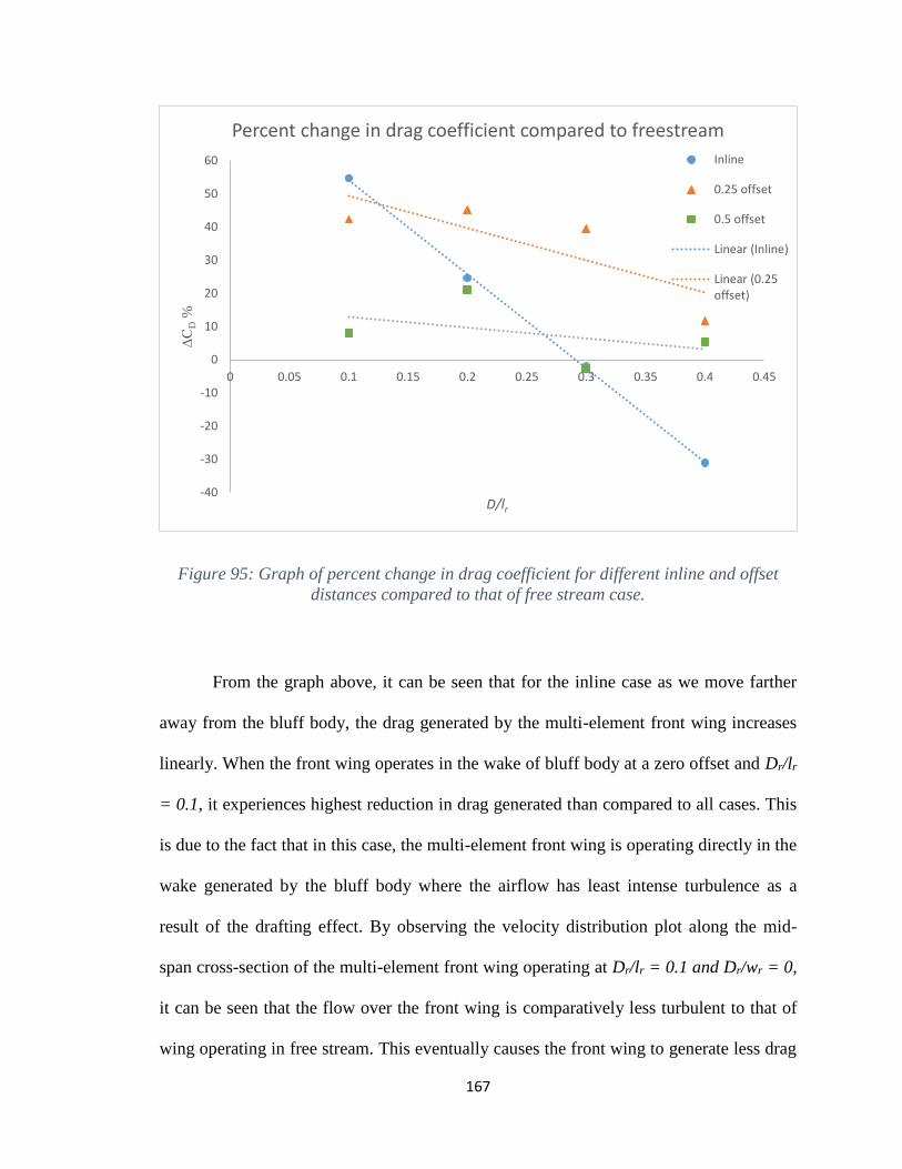
167
Figure 95: Graph of percent change in drag coefficient for different inline and offset
distances compared to that of free stream case.
From the graph above, it can be seen that for the inline case as we move farther
away from the bluff body, the drag generated by the multi-element front wing increases
linearly. When the front wing operates in the wake of bluff body at a zero offset and Dr/lr
= 0.1, it experiences highest reduction in drag generated than compared to all cases. This
is due to the fact that in this case, the multi-element front wing is operating directly in the
wake generated by the bluff body where the airflow has least intense turbulence as a
result of the drafting effect. By observing the velocity distribution plot along the mid-
span cross-section of the multi-element front wing operating at Dr/lr = 0.1 and Dr/wr = 0,
it can be seen that the flow over the front wing is comparatively less turbulent to that of
wing operating in free stream. This eventually causes the front wing to generate less drag
-40
-30
-20
-10
0
10
20
30
40
50
60
0 0.05 0.1 0.15 0.2 0.25 0.3 0.35 0.4 0.45
∆C
D%
D/lr
Percent change in drag coefficient compared to freestream
Inline
0.25 offset
0.5 offset
Linear (Inline)
Linear (0.25offset)

168
force as the flow over it is mostly laminar when compared to free stream. Additionally,
the flow over the front wing also appears to flow at a relatively slower velocity further
reducing the drag generated. Also, as the airflow over the upper surface of the front wing
flows at a relatively slower velocity than free stream, according to Bernoulli’s principle,
there is a less pressure difference between the lower and upper surface also resulting in
lower drag force. Moreover, the pressure distribution plot also shows that most of the
downforce is generated by the main-element.
Figure 96: Velocity distribution plot along the mid-span cross-section of the multi-
element front wing operating at Dr/lr = 0.1 and Dr/wr = 0

169
Figure 97: Zoomed in velocity distribution plot along the mid-span cross-section of the
multi-element front wing operating at Dr/lr = 0.1 and Dr/wr = 0
Figure 98: Pressure distribution plot along the mid-span cross-section of the multi-
element front wing operating at Dr/lr = 0.1 and Dr/wr = 0

170
Furthermore, as seen from the graph, the drag generated by the front wing
increases linearly as we move farther away from the bluff body. By observing the
velocity distribution plots at mid-span cross-section for Dr/lr = 0.1, 0.2, 0.3 and 0.4 for
inline case, it can be seen that as the inline distance increases the front wing moves
further away from wake generated by the bluff body. As the inline distance increases, the
turbulent intensity of the flow increases gradually as the drafting effect created by the
bluff body diminishes. This means that the flow over the front wing is more turbulent and
at higher velocity as seen by the velocity distribution plots. Furthermore, this higher
velocity flow leads to higher pressure difference between the upper and lower surface of
the wing according to Bernoulli’s principle and thus eventually leading to higher value of
drag force. The velocity distribution plots clearly show the gradual increase in the flow
velocity of the airflow flowing over the upper and lower surface of the front wing as the
inline distance increases. For inline distances of Dr/lr = 0.3 and 0.4 the front wing is
operating at such higher velocity turbulent flow that the drag generated by it is higher
than that of in free stream case thus showing a negative value in the graph. The velocity
distribution plot along the mid-span cross-section of the multi-element front wing
operating at Dr/lr = 0.2, 0.3 and 0.4 at Dr/wr = 0 is as shown in following figures.
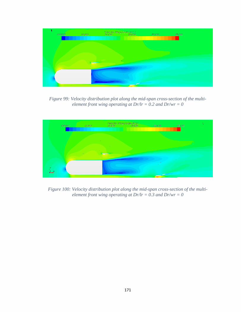
171
Figure 99: Velocity distribution plot along the mid-span cross-section of the multi-
element front wing operating at Dr/lr = 0.2 and Dr/wr = 0
Figure 100: Velocity distribution plot along the mid-span cross-section of the multi-
element front wing operating at Dr/lr = 0.3 and Dr/wr = 0

172
Figure 101: Velocity distribution plot along the mid-span cross-section of the multi-
element front wing operating at Dr/lr = 0.4 and Dr/wr = 0
In addition, it can be seen fromt the graph that for the Dr/lr = 0.1 and Dr/wr = 0,
0.25 and 0.5, there is a difference in the drag reduction when front wing operates in the
wake. For the inline case, as the front wing primarily operates in the wake of lower
velocity less turbulent intense flow, the drag generated is much lower for the inline case
than compared to that with offset distances of 0.25 and 0.5. Furthermore, there are
minimal end-tip vortices acting on the front wing operating in inline as most of the end-
tip vortices are generated by the flow over rear wheels. On the other hand, for offset
distances of Dr/wr = 0.2 and 0.5, the front wing experiences a turbulent flow caused by
the end-tip vortices by the flow over the rear wheels and around the bluff body. Also, by
observing the velocity distribution plots along the top view it can be seen that, for front
wing is placed in a more laminar flow with relatively less oscillations than compared to
other two cases. The bluff body is able to block majority of the turbulent flow in the
inline case and thus resulting in a higher reduction in drag. On contrary, the front wing
when placed at offset distances of Dr/wr = 0.2 and 0.5 experience a relatively more
oscillating flow as seen from the velocity distribution plot. Additionally, to demonstrate

173
the difference of flow over the front wing at different offset distances, an isosurface with
a relative velocity of 10m/s has been plotted for Dr/lr = 0.1 and Dr/wr = 0, 0.25 and 0.5.
From the isosurface it can be clearly seen that when the front wing is placed in inline, the
majority of the front wing is covered by the 10m/s isosurface indicating the majority of
the flow over it is a laminar flow with relatively less turbulence and velocity. Thus,
indicating an effective use of split-stream to reduce drag and gain higher straight-line
speeds. Conversely, by observing the isosurface for offset distances of Dr/wr = 0.2 and
0.5, it appears that as the front wing moves out of the split-stream, the flow over the wing
becomes more turbulent. As the offset distance increases, the effect area that is covered
by the 10m/s isosurface decreases indicating an increase in turbulent flow over the wing.
This increase in turbulent flow along with the end-tip vortices acting on the front wing
causes an increase in drag generated as the offset distance is increased as observed in the
graph.

174
Figure 102: Velocity distribution along the top-view for the multi-element front wing
operating at Dr/lr = 0.1 and Dr/wr = 0
Figure 103: Velocity distribution along the top-view for the multi-element front wing
operating at Dr/lr = 0.1 and Dr/wr = 0.25

175
Figure 104: Velocity distribution along the top-view for the multi-element front wing
operating at Dr/lr = 0.1 and Dr/wr = 0.5
Figure 105: 10 m/s isosurface for the multi-element front wing operating at Dr/lr = 0.1
and Dr/wr = 0

176
Figure 106: 10 m/s isosurface for the multi-element front wing operating at Dr/lr = 0.1
and Dr/wr = 0.25
Figure 107: 10 m/s isosurface for the multi-element front wing operating at Dr/lr = 0.1
and Dr/wr = 0.5

177
Similarly, from the graph in Figure 95 it can be seen that for Dr/lr = 0.2 and Dr/wr
= 0, 0.25 and 0.5, there is a significant difference in the drag reduction. For an offset
distance of Dr/wr = 0.2, the multi-element front wing experiences a higher reduction in
drag than compared to the other offset distances. By observing the velocity distribution
plots from top view, it can be seen that just as for inline Dr/lr = 0.1, most of the surface
area of the front wing for Dr/lr = 0.2 and Dr/wr = 0.25 is operating in the wake of the
bluff body where the flows relatively slow and less turbulent as the majority of the
turbulent flow is blocked by the rear wheels of the bluff body. On the other hand, for the
inline Dr/lr = 0.2 case, the front wing is placed in a higher turbulent flow as it operates
directly behind the wake generated by the diffuser. This leads to a higher value of drag
force generated. Also, when the front wing is operating in the wake at Dr/lr = 0.2 and
Dr/wr = 0.5 not only it operates directly in the turbulent wake generated by the bluff body
and its rear wheel but also outside the wake of bluff body ultimately resulting in
generation of higher drag force. The velocity distribution plots and an isosurface of 10m/s
shows the multi-element front wing operating in wake at Dr/lr = 0.2 and Dr/wr = 0, 0.25
and 0.5 in following figures.

178
Figure 108: Velocity distribution along the top-view for the multi-element front wing
operating at Dr/lr = 0.2 and Dr/wr = 0
Figure 109: Velocity distribution along the top-view for the multi-element front wing
operating at Dr/lr = 0.2 and Dr/wr = 0.25

179
Figure 110: Velocity distribution along the top-view for the multi-element front wing
operating at Dr/lr = 0.2 and Dr/wr = 0.5
Figure 111: 10 m/s isosurface for the multi-element front wing operating at Dr/lr = 0.2
and Dr/wr = 0.

180
Figure 112: 10 m/s isosurface for the multi-element front wing operating at Dr/lr = 0.2
and Dr/wr = 0.25

181
Figure 113: 10 m/s isosurface for the multi-element front wing operating at Dr/lr = 0.2
and Dr/wr = 0.5
Furthermore, it can be seen from the graph in Figure 95, that a similar trend is
followed for the drag generated by the front wing operating in wake. Thus to summarize
in general it appears that, if the inline distance between the multi-element front wing
operating in the wake is increased, there is an increase in the drag generated by the wing.
In other words, for a zero offset or when the front wing is operating directly behind the
bluff body, for every increase in the inline distance the drag force generated increases
linearly. However, the various offset distances does not have a linear effect on the drag
force generated. For offset distance of Dr/wr = 0.25, the drag generated is higher than that
for an offset distance of Dr/wr = 0.5. As for Dr/wr = 0.25, the rear wheels and the bluff
body blocks majority of the turbulent flow and as a result the front wing operates in a

182
relatively less turbulent flow. Whereas, for the Dr/wr = 0.5, the front wing primarily
operates in a relatively turbulent flow outside the wake generated by the bluff body.
Moreover, the studies for the multi-element front wing operating in wake show the
downstream wing is significantly affected by the up-wash flow field from the leading
racecar. Also, from the trend line in the graph it can be seen that as we move away from
the bluff body, the drag reduction decreases thus indicating an increase in drag
experienced by the front wing. However, the leading racecar also creates a drafting effect
which can be used to get as a tow and improve straight-line speeds of following racecar.

183
9. Conclusion
A three-dimensional computational analysis of a two-element front wing for a
Formula One racecar to investigate the effect of various parameters such as turbulence
modelling, ground clearance, angle of attack and operating in wake of a generic bluff
body has been successfully conducted in the present study. The airfoil used for this study
is a highly cambered double-element Formula One front wing consisting of two elements
in a single slotted flap configuration. The main element and the flap are a modified
NASA GA (W) profile of type LS (1)-0413 profile having a total chord length of 380mm.
The computational analysis has been conducted using a Reynolds Averaged Navier-
Strokes (RANS) model and it successfully has been able to predict the three-dimensional
flow over the double-element front wing. The current study aimed to determine the
appropriate use of meshing model for a three-dimensional study by investigating the
effectiveness of the structured trimmer and the unstructured polyhedral meshing model.
By using a thin layer prism layer mesher and same reference values for both the trimmer
and polyhedral meshing model, it has been observed that for a three-dimensional multi-
element front wing, the unstructured polyhedral meshing model has been able to provide
a more refined volume mesh than compared to the structured trimmer meshing model
using the same level of refinement.
Furthermore, considering the difficulties in duplicating the real operating conditions
for a turbulent flow in a computational analysis, the present study also aimed at
determining the predictive capability of the different turbulence models. Thus, the
predictive capability of the standard k- ω Shear Stress Transport (SST) and the one

184
equation Spalart-Allmarus turbulence model to predict the three-dimensional flow over a
multi-element front wing in ground effect has also been investigated. The aerodynamics
of a double-element front wing operating in ground effect has been studied at three
different ground clearances of H/c = 0.224, 0.09 and 0.05, representing the downforce
enhancement and downforce reduction regions. Also, to get more realistic results, a
moving ground simulation has been used. It has been observed that for medium and low
ground clearances of H/c = 0.224 and 0.09, both the turbulence models has been able to
predict the aerodynamic forces generated equally. There is no significant difference in
accuracy for predicting the lift and drag forces generated by the wing for both the models.
However, for very low ground clearances of H/c = 0.05, the standard k- ω Shear Stress
Transport (SST) proved to be more accurate when compared to the one equation Spalart-
Allmarus turbulence model.
In addition, the aerodynamics of a multi-element front wing for a Formula One
racecar operating in a free stream has also been determined in this study. From the results
it has been observed that for a three-dimensional flow, the multi-element front wing in
free stream behaves as an inverted airfoil generating negative lift or downforce with the
help of Bernoulli’s principle. Also, to determine the optimum operating conditions for the
multi-element front wing, it has been studied in a varying ground clearance and angle of
attack with a moving ground simulation. From the results it has been observed that, for a
three-dimensional flow when subjected to decreasing ground clearance, the multi-element
front wing exhibits two distinct regions of downforce generation. A force enhancement
region for medium ground clearances where downforce behaves as a function of ground
clearance i.e. for every decrease in ground clearance there is a corresponding increase in
185
downforce generated and a force reduction region for very low ground clearances where
the downforce generated reduces for any further decrease in ground clearance. By
observing the flow distribution plots, the reason for the downforce reduction is due to the
separation of boundary layers at the trailing edge of wing. This separation of boundary
layers is a result of boundary layers at trailing edge not capable of withstanding the
adverse pressure gradient associated with accelerated flow at very low ground clearances.
Also, the three-dimensional flow characteristics for increasing overall angle of attack
with simultaneous decrease in ground clearance indicate that ground plane has more
impact in determining the downforce generated for lower values of overall angle of
attack. However, for very low values of ground clearances and higher values of angle of
attack, the downforce generated increase as the overall angle of attack has a significantly
more impact.
Additionally, the aerodynamics of a double-element front wing operating in the wake
of a generic bluff body has also been investigated in the current study. To study the effect
of drafting by the wake of a leading racecar, the front wing has been studied at different
inline and offset distances by conducting a three-dimensional computational analysis. By
studying the front wing at different inline and offset distances in the wake of a bluff
body, it has been observed that the bluff body does create a drafting effect and has
significant impact in determining the aerodynamic forces generated by it. When the front
wing is placed at zero offset, for every increase in inline distance, the drag increases
linearly. This indicates that as we move away from the bluff body the effectiveness of
drafting effect reduces. Thus to gain higher reduction in drag, the following racecar needs
to operate in close proximity to that of leading racecar. Conversely, by observing the

186
results for different offset distances, it has been found that the drag generated does not
behave linearly. The wake generated by the rear wheels and rear wing plays a significant
impact in determining the drag force generated by the front wing. When the front wing is
placed in the region of less turbulent flow generated as a result of rear wheels blocking
majority of turbulent flow, a higher reduction in drag is observed. Similarly, when the
front wing is placed in the more turbulent wake generated by the rear diffuser, it fails to
achieve higher drag reduction. Thus, indicating the drag generated for front wing
operating at different offset distances in the wake is dependent on the flow generated by
the bluff body.

187
Appendix
Airfoil profile:
Table 4: Coordinates for front wing (Airfoil Tools n.d.)
x y x y
1.0000 0.0603 0.0000 0.0000
0.9900 0.0573 0.0010 0.0079
0.9799 0.0543 0.0020 0.0109
0.9599 0.0484 0.0051 0.0173
0.9399 0.0426 0.0101 0.0232
0.9199 0.0370 0.0151 0.0270
0.8999 0.0315 0.0201 0.0299
0.8498 0.0183 0.0251 0.0312
0.7998 0.0060 0.0301 0.0321
0.7498 -0.0056 0.0351 0.0329
0.6997 -0.0163 0.0401 0.0336
0.6497 -0.0261 0.0451 0.0344
0.5997 -0.0351 0.0501 0.0352
0.5497 -0.0434 0.0551 0.0359
0.4996 -0.0508 0.0601 0.0367
0.4496 -0.0574 0.0701 0.0379
0.3996 -0.0631 0.0801 0.0392
0.3496 -0.0679 0.0902 0.0404

188
0.2996 -0.0721 0.1002 0.0413
0.2496 -0.0753 0.1202 0.0432
0.1996 -0.0771 0.1402 0.0446
0.1796 -0.0763 0.1602 0.0457
0.1596 -0.0744 0.1802 0.0465
0.1396 -0.0713 0.2002 0.0473
0.1197 -0.0672 0.2501 0.0489
0.0997 -0.0619 0.3001 0.0504
0.0897 -0.0588 0.3501 0.0514
0.0797 -0.0544 0.4001 0.0519
0.0698 -0.0518 0.4501 0.0521
0.0598 -0.0479 0.5001 0.0517
0.0548 -0.0458 0.5501 0.0509
0.0498 -0.0436 0.6001 0.0496
0.0448 -0.0414 0.6500 0.0479
0.0398 -0.0392 0.7000 0.0456
0.0348 -0.0368 0.7500 0.0429
0.0298 -0.0344 0.8000 0.0409
0.0249 -0.0319 0.8500 0.0412
0.0199 -0.0293 0.9000 0.0446
0.0149 -0.0266 0.9200 0.0468
0.0099 -0.0228 0.9400 0.0496
0.0049 -0.0168 0.9600 0.0527

189
0.0020 -0.0107 0.9800 0.0563
0.0010 -0.0076 0.9900 0.0583
0.0000 0.0000 1.0000 0.0603

190
Studies conducted in relevant field of interest
Table 5: Relevant Studies
No Year
Wing Element
Profile
Type Dimensionality Parameters studied
Front Rear Single Multi Computational Experimental 2-D 3-D Ground Clearance Angle of attack Reynolds No. Wake
1 2016 ✔ ✔ S1223 ✔ ✔ ✔ ✔
2 2011 ✔ ✔ FX 63-137 ✔ ✔ ✔ ✔
3 2011 ✔ ✔ Designed by Pakkam ✔ ✔ ✔ ✔
4 2010 ✔ ✔ Designed by Mr. Rudis ✔ ✔ ✔ ✔
5 2009 ✔ ✔ NASA GA(W) LS(1)-0413 ✔ ✔ ✔
6 2009 ✔ ✔ NASA GA(W) LS(1)-0413 ✔ ✔ ✔
7 2008 ✔ ✔ NACA 0012 ✔ ✔ ✔
8 2008 ✔ ✔ S1223 ✔ ✔ ✔
9 2008 ✔ ✔ NASA GA(W) LS(1)-0413 ✔ ✔ ✔ ✔
10 2006 ✔ ✔ NASA GA(W) LS(1)-0413 ✔ ✔ ✔
11 2006 ✔ ✔ Toyota Atlantic Series ✔ ✔ ✔
12 2005 ✔ ✔ NASA GA(W) LS(1)-0413 ✔ ✔ ✔ ✔ ✔ ✔
13 2005 ✔ ✔
LNV109A
✔ ✔ ✔ ✔ ✔
EA23
S1223
NACA 9315
14 2004 ✔ ✔ NASA GA(W) LS(1)-0413 ✔ ✔ ✔
15 2004 ✔ ✔ NASA GA(W) LS(1)-0413 ✔ ✔ ✔
16 2004 ✔ ✔ ✔ Formula Mazda ✔ ✔ ✔ ✔
17 2004 ✔ ✔ NASA GA(W) LS(1)-0413 ✔ ✔ ✔
18 2003 ✔ ✔ NASA GA(W) LS(1)-0413 ✔ ✔ ✔
19 2000 ✔ ✔ NASA GA(W) LS(1)-0413 ✔ ✔ ✔ ✔
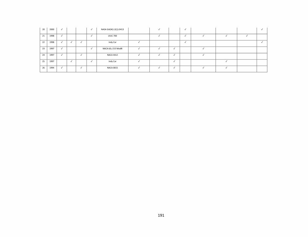
191
20 2000 ✔ ✔ NASA GA(W) LS(1)-0413 ✔ ✔ ✔
21 1998 ✔ ✔ UIUC 700 ✔ ✔ ✔ ✔ ✔
22 1998 ✔ ✔ ✔ Indy Car ✔ ✔ ✔
23 1997 ✔ ✔ NACA 632-215 ModB ✔ ✔ ✔ ✔
24 1997 ✔ ✔ NACA 4412 ✔ ✔ ✔ ✔
25 1997 ✔ ✔ Indy Car ✔ ✔ ✔
26 1994 ✔ ✔ NACA 0015 ✔ ✔ ✔ ✔ ✔

192
References
[1] Katz, J. (2006). Aerodynamics of Racecars. Annual Review of Fluid Mechanics, (pp. 27-
63).
[2] Seljak, G. (2008). Racecar Aerodynamics. Ljubljana.
[3] Fédération Internationale de l’Automobile. (2016, February 27). 2016 F1 Technical
Regulations. Retrieved from http://www.fia.com/regulation/category/110
[4] Gunston, B. (2004). The Cambridge aerospace dictionary. Cambridge, UK, New York:
Cambridge University Press.
[5] Selig, M. S., Guglielmo, J. J., Broeren, A. P., & Giguere, P. (1995). Summary of Low-
Speed Airfoil Data. Virgia Beach: Virgina: Solar Tech Publications.
[6] Kieffer, W., Moujaes, S., & Armbya, N. (2004). CFD study of section characteristics of
Formula Mazda racecar wings. Las Vegas: Elsevier Ltd.
[7] Ranzenbach , R., & Barlow , J. B. (1994). Two-Dimensional Airfoil in Ground Effect, An
Experimental and Computational Study. Motorsport Engineering Conference. 1, pp. 241-
249. SAE International.
[8] Ranzhanbach, R., & Barlow, J. B. (1997). Cambered Airfoil in Ground Effect. AIAA.
[9] Ranzenbach, R., Barlow, J. B., & Diaz, R. H. (1997). Mulit-Element Airfoil in Ground
Effect-An Experimental and Computational Study. AIAA.

193
[10] Mokhtar, W. A. (2005). A Numerical Study of High-Lift Single Element Airfoils
With Ground Effect For Racing Cars. Norfolk: SAE International .
[11] Mokhtar, W., & Lane, J. (2008). Racecar Front Wing Aerodynamics. SAE
International.
[12] Mokhtar, W. A. (2008). Aerodynamics of High-Lift Wings with Ground Effect for
Racecars. Sault Ste Marie: SAE International .
[13] Mokhtar, W., & Durrer, S. (2016). A CFD Analysis of a Racecar Front Wing in
Ground Effect. 2016 ASME North Central Section Conference.
[14] Zerihan, J., & Zhang, X. (2000). Aerodynamics of a Single Element Wing in
Ground Effect. Journal of Aircraft, 1058-1064.
[15] Mahon, S., & Zhang, X. (2004). Computational Analysis of Pressure and Wake
Characteristics of an Aerofoil in Ground Effect. Journal of Fluids Engineering.
[16] Kuya, Y., Takeda, K., Zhang, X., Beeton, S., & Pandaleon, T. (2009). Flow
Separation Control of a Racecar Wing With Vortex Generators in Ground Effect. Journal
of Fluids Engineering.
[17] Genua, E. (2009). A CFD Investigation into Ground Effect Aerodynamics.
Netherlands: Delft Unniversity of Technology.
[18] Price, T. A. (2011). 3D CFD on an Open Wheel Racecar Front Wing in Ground
Effects . San Luis Obispo : California Polytechnic State University.

194
[19] Jasinski, W. J., & Seilg, M. S. (1998). Experimental Study of Open-Wheel Race-
Car Front Wings. Illinois: SAE International.
[20] Zhang, X., & Zerihan, J. (2003). Aerodynamics of a Double-Element Wing in
Ground Effect. AIAA, 1007-1016.
[21] Mahon, S., & Zhang, X. (2006). Computational Analysis of an Inverted Double-
Element Wing in Ground Effect. Suthampton: Univeristy of Southampton.
[22] Zhang, X., & Zerihan, J. (2004). Edge Vortices of a Double-Element Wing in
Ground Effect. Journal of Aircraft, 41 No. 5.
[23] Zerihan, J., & Zhang, X. (2000). Aerodynamics of Gurney Flaps on a Wing in
Ground Effect. American Institute of Aeronautics and Astronautics.
[24] Katz , J., Lou, H., Baum, J., & Löhner , R. (1998). Viscous-Flow Simulation of an
Open-Wheel Racecar. Motorsports Engineering Conference Proceedings, 1: Vehicle
Design and Safety. Dearbon.
[25] Zhang, X., Toet, W., & Zerihan, J. (2006). Ground Effect Aerodynamics of
Racecars. Applied Mechanics Review, 33-47.
[26] Zerihan, J., & Zhang, X. (2000). Aerodynamics of Gurney Flaps on a Wing in
Ground Effect. American Institute of Aeronautics and Astronautics.
[27] Wilson, M. R., Dominy, R. G., & Straker, A. (2008). The Aerodynamic
Characteristics of a Racecar Wing Operating in a Wake. SAE International.
195
[28] Soso, M. D., & Wilson, P. A. (2005). Aerodynamics of Wing in Ground Effect in
Generic Racecar Wake Flows. Southampton, UK: School of Engineering Science,
Univeristy of Southampton.
[29] Guarro, M. D. (2010). Wing Efficiency of Racecars. Santa Cruz: Univeristy of
California.
[30] Gopalarathnam, A., Selig, M. S., & Frank, H. (1997). Design of High-Lift Airfoils
for Low Aspect Ratio Wings with Endplates. 15th Applied Aerodynamics Conference.
Atlanta.
[31] Pakkam, S. S. (2011). High Downforce Aerodynamics for Motorsports . North
Carolina: Norht Carolina State Univeristy.
[32] Gogel , D., & Sakurai, H. (2006). The Effects of End Plates on Downforce in Yaw.
Dearbon: SAE international.
[33] Airfoil Tools. (n.d.). Retrieved 01 31, 2017, from Airfoil Tools:
http://www.airfoiltools.com/
[34] Versteeg, H. K., & Malalasekera, W. (2007). An Introduction to Computational
Fluid Dynamics. Harlow, England: Pearson Prentice Hall.
[35] Georgiadis, N. J., Yoder, D. A., & Engblom, W. A. (2006). Evaluation of
Modified Two-Equation Turbulence Models forJet Flow Predictions. 44th AIAA
Aeroscapce Sciences Meeting and Exhibition. Reno, Nevada.

196
[36] Menter, F. R. (1993). Zonal Two Equation k- ε Turbulence Models for
Aerodynamic Flows. 24th Fluid Dynamics Conference. Orlando, Florida: AIAA.
[37] Spalart, P., & Allmarus, S. (1992). The One Equation Turbulence Model for
Aerodynamic Flow. AIAA 30th Aerospace Sciences Meeting and Exhibition. Reno,
Nevada.
[38] Mokhtar, W. and Kachare, S. (2017). Predictive Capability of the k-ωSST and
Spalart-AllmarusTurbulence Model for a Double-Element Front Wing in Ground Effect-
A CFD Analysis. IJESIT 55-63.


