A CFD Database for Airfoils and Wings at Post-Stall Angles ofAttack

Justin Petrilli,∗ Ryan Paul,† Ashok Gopalarathnam,‡

Department of Mechanical and Aerospace EngineeringNorth Carolina State University, Raleigh, NC 27695-7910

andNeal T. Frink§

NASA Langley Research Center, Hampton, Virginia, 23681

This paper presents selected results from an ongoing effort to develop an aerodynamic database fromReynolds-Averaged Navier-Stokes (RANS) computational analysis of airfoils and wings at stall andpost-stall angles of attack. The data obtained from this effort will be used for validation and re-finement of a low-order post-stall prediction method developed atNCSU, and to fill existing gaps inhigh angle of attack data in the literature. Such data could have potential applications in post-stallflight dynamics, helicopter aerodynamics and wind turbine aerodynamics. An overview of the NASATetrUSS CFD package used for the RANS computational approachis presented. Detailed results forthree airfoils are presented to compare their stall and post-stallbehavior. The results for finite wingsat stall and post-stall conditions focus on the effects of taper-ratio and sweep angle, with particular at-tention to whether the sectional flows can be approximated using two-dimensional flow over a stalledairfoil. While this approximation seems reasonable for unswept wings even at post-stall conditions,significant spanwise flow on stalled swept wings preclude the use of two-dimensional data to modelsectional flows on swept wings. Thus, further effort is needed in low-order aerodynamic modeling ofswept wings at stalled conditions.

NomenclatureAR = aspect ratioa = VGRID stretching/growth factorb = VGRID stretching/growth factorCFD = computational fluid dynamicsCd = airfoil or section drag coefficientC f = skin friction coefficientCL = wing lift coefficientCl = airfoil or section lift coefficientCm = airfoil or section pitching moment coefficient about the quarter-chordCp = pressure coefficientcre f = reference chord lengthRe = Reynolds number based on airfoil chordS A = Spalart-Allmaras turbulence modelT E = trailing edge∆t = physical time stepU∞ = Freestream reference velocityy+ = non-dimensional wall distance∆zi = height of theith viscous layerα = angle of attack, degΛ = angle of sweepback, degλ = taper ratio

∗Graduate Research Assistant, Box 7910, jlpetril@ncsu.edu. Student Member, AIAA†Graduate Research Assistant, Box 7910, rcpaul@ncsu.edu. Student Member, AIAA‡Associate Professor, Box 7910, ashokg@ncsu.edu, (919) 515-5669. Associate Fellow, AIAA§Aerospace Engineer, Configuration Aerodynamics Branch, MS499. Associate Fellow, AIAA

https://ntrs.nasa.gov/search.jsp?R=20140000500 2018-07-11T13:45:06+00:00Z

I. IntroductionAirfoil lift and moment data in the low angle of attack regimeis readily available from a multitude of sources- fromAbbott and von Doenhoff [1] and those from the University of Stuttgart [2] and University of Illinois at Urbana-Champaign [3,4,5], to modern computational approaches designed to predict sectional aerodynamic characteristicsbased on arbitrary input geometry, such as XFOIL [6]. For many applications, data in this linear regime is sufficient.However, fields such as wind turbine aerodynamics, helicopter aerodynamics and post-stall flight dynamics of fixed-wing aircraft require data to extend beyond aerodynamic stall. Efforts have been made in the wind turbine communityand the helicopter aerodynamics community to extend airfoil data into the post-stall regime. In both wind turbine andhelicopter aerodynamics, local blade sections close to theroot of the rotor may experience very high angles of attack.Models for airfoil force and moment coefficients at high angle of attack conditions have been developed experimentally[7,8], which has led to researchers proposing empirical models based on flat plate theory [9]. The empirical modelsdeveloped from experiment require that both the maximumCl and the correspondingαstall at which this lift coefficientoccurs be known reliably before theoretical flat plate data may be fitted to extend the data well into post-stall.

Very little data exists in the literature covering the stallbehavior of finite wings, especially that which extendsdeep into post-stall. Published work in post-stall wing aerodynamics often covers general stall behavior, dependenton factors such as planform, without providing detailed force and moment data beyond initial stall [10]. Some studiespropose empirical methods based on theory to extend existing force and moment coefficient data-sets deep into post-stall taking into account 3D effects with some correction for aspect ratio [8]. An interesting, purely experimental study,that covers the stall of both a 2D airfoil section and 3D wingsof various aspect ratios was performed by Ostowari andNaik in 1985 [11]. The study presented consistent lift coefficient versus angle of attack data for various NACA 44XXseries airfoils and 3D rectangular wings with a range of aspect ratios having the same airfoils as cross sections.

A database of post-stall airfoil and wing data, with a similar scope to the Ostowari and Naik study, was desiredpartly to address this dearth of data in the literature, but primarily to support a local effort within the Applied Aero-dynamics Group at North Carolina State University. The ongoing effort involves developing a low-order model ofpost-stall aerodynamics for finite wings via use of existinglinear low-order methods (VLM, Weissinger or LLT) cor-rected for nonlinear sectional airfoil behavior. Corrections are accomplished via a decambering approach used tomimic the nonlinear aerodynamics caused by flow separation.Details of the development of the low-order methodmay be found in Ref. [12], with the current status pertaining to its use in real-timesimulation of aircraft flight dynam-ics described in Ref. [13]. In addition to geometry information, the low-order post-stall model requires sectional 2Dairfoil data as input for each of the control points. This sectional input data (Cl −α, Cd−α, andCm−α curves) definesthe convergence criteria for the low-order post-stall calculation for finite wings. Outputs include the total aerodynamicforce and moment coefficients and spanwise distributions ofthese coefficients.

Figure1 describes the relationship between the low-order method and the higher order Computational Fluid Dy-namics (CFD) effort, and how the results from the latter are to be used for initial validation and further refinement ofthe former. Two dimensional CFD is performed on airfoil sections, and the outputs are used as inputs to the low-ordermethod. The 3D geometries utilizing the same 2D cross section are run in both CFD and the low-order method.Theresults are then compared on the basis of total force/moments and spanwise force/moment distributions. CFD solu-tions and accompanying flow visualizations allow for further development and refinement of the low-order method.Comparisons between the low-order method and CFD are beyondthe scope of this paper. This paper aims to discussthe methodology used in generating CFD solutions of airfoils and wings in post-stall angles of attack and to presentthe results in this regime as dependent on geometry and flow conditions.

This paper begins by describing the CFD software package that was chosen to generate consistent flow solutionsfor airfoils and wings. The methodology developed to effectively use the CFD package is presented next - fromgenerating usable geometry, creating a suitable grid over the computational domain, running the flow-solver, checkingsolution convergence, and post-processing to extract desired quantities from the outputs. The 2D and 3D results arepresented which show effects from geometry, including wingsweep, and flow parameters. Selected results are shownin more detail using flow visualization and/or spanwise local lift coefficient distributions.

2 of 18

American Institute of Aeronautics and Astronautics

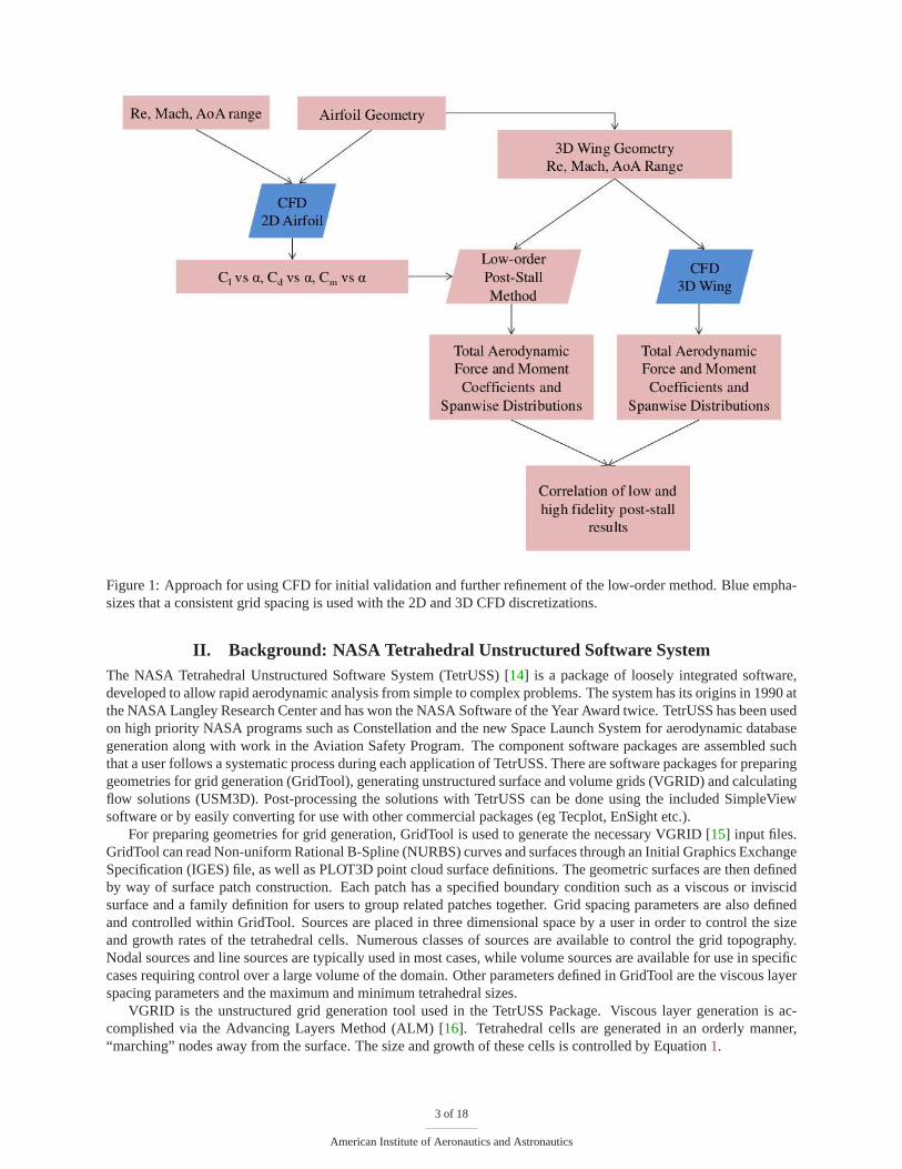
Figure 1: Approach for using CFD for initial validation and further refinement of the low-order method. Blue empha-sizes that a consistent grid spacing is used with the 2D and 3DCFD discretizations.

II. Background: NASA Tetrahedral Unstructured Software SystemThe NASA Tetrahedral Unstructured Software System (TetrUSS) [14] is a package of loosely integrated software,developed to allow rapid aerodynamic analysis from simple to complex problems. The system has its origins in 1990 atthe NASA Langley Research Center and has won the NASA Software of the Year Award twice. TetrUSS has been usedon high priority NASA programs such as Constellation and thenew Space Launch System for aerodynamic databasegeneration along with work in the Aviation Safety Program. The component software packages are assembled suchthat a user follows a systematic process during each application of TetrUSS. There are software packages for preparinggeometries for grid generation (GridTool), generating unstructured surface and volume grids (VGRID) and calculatingflow solutions (USM3D). Post-processing the solutions withTetrUSS can be done using the included SimpleViewsoftware or by easily converting for use with other commercial packages (eg Tecplot, EnSight etc.).

For preparing geometries for grid generation, GridTool is used to generate the necessary VGRID [15] input files.GridTool can read Non-uniform Rational B-Spline (NURBS) curves and surfaces through an Initial Graphics ExchangeSpecification (IGES) file, as well as PLOT3D point cloud surface definitions. The geometric surfaces are then definedby way of surface patch construction. Each patch has a specified boundary condition such as a viscous or inviscidsurface and a family definition for users to group related patches together. Grid spacing parameters are also definedand controlled within GridTool. Sources are placed in threedimensional space by a user in order to control the sizeand growth rates of the tetrahedral cells. Numerous classesof sources are available to control the grid topography.Nodal sources and line sources are typically used in most cases, while volume sources are available for use in specificcases requiring control over a large volume of the domain. Other parameters defined in GridTool are the viscous layerspacing parameters and the maximum and minimum tetrahedralsizes.

VGRID is the unstructured grid generation tool used in the TetrUSS Package. Viscous layer generation is ac-complished via the Advancing Layers Method (ALM) [16]. Tetrahedral cells are generated in an orderly manner,“marching” nodes away from the surface. The size and growth of these cells is controlled by Equation1.

3 of 18

American Institute of Aeronautics and Astronautics

∆zi+1 = ∆z1

[

1+ a(1+ b)i]i

(1)

In this equation, the height of theith layer is determined by an initial spacing parameter,∆z1, and two stretching/growthfactorsa andb. Once the height of theith layer reaches the size of the background sources specified bythe user inGridTool, no more cells are formed and viscous layer generation is complete. After the viscous layers are generated,VGRID then utilizes the Advancing Front Method (AFM) [17] for the generation of the inviscid portion of the volumegrid. VGRID can not always close the grid completely. When this occurs, a slower but more robust auxiliary codecalled POSTGRID is used to complete the formation of the remaining tetrahedral cells.

The flow solver at the core of the TetrUSS package is USM3D [18]. USM3D is a parallelized, tetrahedral cell-centered, finite volume Reynolds Averaged Navier-Stokes (RANS) flow solver. It computes the finite volume solutionat the centroid of each tetrahedral cell and utilizes several upwind schemes to compute inviscid flux quantities acrosstetrahedral faces. USM3D has numerous turbulence models implemented for use; the Spalart-Allmaras (SA) one-equation model and Menter Shear Stress Transport (SST) two equation model were used in this study. Some additionalcapabilities that USM3D has implemented are dynamic grid motion and overset grids.

III. Methodology: Developing the Aerodynamic DatabaseThe aerodynamic database is desired to have high fidelity flowsolutions for a wide variety of 2D airfoils and 3Dgeometries. Flow solutions would include a large range of angles of attack to encompass pre-stall, stall and post-stallflow regimes. The data gained from these simulations will be vital in assisting the further development and validationof the low-order method mentioned in the introduction as well as to fill gaps in the currently available high angle ofattack aerodynamic data for arbitrary geometries. An efficient process to go from a geometry to a converged flowsolution was developed and is discussed in the following sub-sections.

A. Geometry Generation

Traditional Computer Aided Design (CAD) software would be more than adequate for the creation of the desiredgeometries, however these tools are not geared specificallytowards the modeling of wings and airfoils. Understandingthis, the recently released parametric modeling tool, OpenVehicle Sketch Pad (OpenVSP) [19], was chosen as thegeometry generation tool. A flow chart showing the process ofgeometry generation can be seen in Figure2. OpenVSPis a modeling package developed and released by NASA LangleyResearch Center in Hampton, Virginia. The uniqueconcept that OpenVSP provides is that it allows a user to dragand drop generic aircraft components (such as a wing)into the modeling area, and directly manipulate familiar geometric parameters. Consequently, it is simple to insert awing, change its root chord, tip chord, span, etc. and view the resulting geometry in real time. Aerodynamic referencequantities can also be automatically calculated for the user. Airfoils cross section generation is also simplified. Auser can select any 4 or 5 digit series NACA airfoil or load in aformatted airfoil coordinate file for use on any liftingsurface.

The 3D wing and corresponding airfoil for each case to be analyzed were generated in OpenVSP. In order to readthe geometry into GridTool, the file must be in the IGES format. Vehicle Sketch Pad does not output IGES files,thus each geometry must be exported as a Rhino3D formatted file. The Rhinoceros NURBS modeling package wasused to convert the geometry into the necessary IGES file as well as make small modifications to the geometry. Somegrid generation failures were encountered due to how OpenVSP closes the trailing edge of the wing/airfoil geometries(it always forces a sharp trailing edge). In some cases the sharpness had to be removed to ensure successful gridgeneration.

4 of 18

American Institute of Aeronautics and Astronautics

Figure 2: Process of geometry generation to grid generation

B. Grid Generation

Grid generation parameters were generalized such that, between different geometries, parameters such as source place-ment and viscous spacing had minimal required changes. Thismeant that from initial geometry generation to a com-pleted grid would require only a matter of hours. Establishing this commonality and routine for grid generation enabledthe generation of adequate grids for many configurations in ashort time span. An example placement of sources fora simple tapered wing is shown in Figure3. A series of line sources are utilized, in the spanwise direction of eachwing at differing chord-wise locations. Anisotropic stretching [20] as high as 10:1 was used near the root of the wing,transitioning to isotropic cells near the wing tips. For viscous tetrahedral layer generation, the height of the first layer(∆z1) is Reynolds number dependent. A viscous layers spacing tool called USGUTIL, was used to determine theheight of the initial viscous layer. In order to have adequate number of cells in the viscous layers, they+ of the firstnode was set to be 3, this would ensure that they+ of the first cell center would be less than 1 (approx. 0.75) as isrequired for a fully viscous Navier-Stokes solution. The values used for the grid growth parameters (a andb) in Eq.1 were 0.15 and 0.02 respectively [20]. A grid sensitivity study was performed on a rectangular wing with aspectratio of 12 to determine adequate grid sizing. It was found that a grid sizing of 5–9 million tetrahedral cells showedchanges inCL,max of approximately 0.02 between the grids. This method of gridgeneration was applied to all 3D winggeometries with the typical grids averaging between 9–12 million tetrahedral cells.

For airfoil calculations, a quasi 2D grid was generated on a constant-chord, short-span wing, between two reflectionplane boundary condition patches. Figure4 shows a completed grid for an NACA 0012 airfoil. A general goal wasset to maintain very similar grid density between the 3D winggrids and the airfoil grids. This is necessary becausethe airfoil results were being used as input data into the low-order method discussed in the introduction while the 3Dwing results from USM3D were being used to assess the accuracy of the low-order method (Figure1). Therefore aseparate grid sensitivity study was not performed specifically for airfoils. Typical airfoil grids were on the order of300,000 tetrahedral cells and were generated using a nearlyidentical source placement as the 3D wing.

C. Flow Solution Generation

All solutions with the USM3D solver were computed with time-accurate Reynolds-Averaged Navier-Stokes (RANS).The limitations of RANS for modeling massively separated flows are well known. The more preferred Detached EddySimulation (DES) modeling will provide better physical representation of 3D separated flow, but with an order-of-magnitude more expense. Since this investigation requiresgeneration of many flow solutions, the initial focus is todetermine if time-accurate RANS can provide sufficient engineering accuracy for capturing the salient aerodynamiccharacteristics of wings at stall and post-stall conditions. Furthermore, a consistent modeling is desired between the2D airfoils and 3D wings.

All computations were advanced at a characteristic time step of ∆t∗ = ∆t · U∞/cre f = 0.02 using a second or-der time-accurate scheme with three-point backward differencing and physical time stepping. The number of sub-iterations for each time step was set to between 10 and 15 to ensure adequate sub-iteration convergence. The Spalart-

5 of 18

American Institute of Aeronautics and Astronautics

Figure 3: Screen capture of GridTool source placementon a tapered wing.

Figure 4: Screen capture of airfoil grid.

Allmaras (SA) [21] one equation turbulence model was used almost exclusively, however some simulations wereperformed with the two equation SST turbulence model to understand the difference in final solution quantities. Thesolver was run on both a NASA Langley computer cluster and theNorth Carolina State University High PerformanceComputing (NCSU HPC) cluster. Making use of USM3D’s parallel computation capabilities, each grid was parti-tioned into 28-64 equal zones which could be loaded onto 28–64 individual processors, reducing calculation timessignificantly. To further increase productivity, a series of Unix scripts were developed to generate the required inputfiles for job submission and minor post-processing of completed jobs.

D. Solution Convergence

Convergence of the solutions was monitored by generating convergence plots such as that seen in the Figure5. Unixscripts were used to compile all of the convergence information contained in the USM3D output files into a Tecplotformat. Each plot showed the logarithm of the residual over each iteration and the changes in the aerodynamic co-efficients. The criteria for a fully converged solution was for each plot to show a leveling off of the quantities underconsideration. These plots allowed for rapid determination of whether any given solution had reached a convergedstate (Figure5a) or if the solution had attained an unsteady solution shown by oscillatory convergence (Figure5b).

0 1 2 3 4

x 104

0

0.5

1

1.5

2

2.5

3

3.5

iteration

Cl

a) Smooth convergence,α = 30deg.

0 0.5 1 1.5 2 2.5 3

x 104

0

0.5

1

1.5

2

2.5

3

3.5

iteration

Cl

b) Oscillatory convergence,α = 48deg.

Figure 5: Typical USM3D convergence of lift coefficient for an airfoil. NACA 4415, USM3D/SA, RE= 3 million,M∞ = 0.2.

6 of 18

American Institute of Aeronautics and Astronautics

E. Post-Processing

After solution convergence was verified, the data is processed so that total forces and moments, the spanwise distri-bution of forces and moments, and flow visualization may be studied. As was previously mentioned, in some casesan oscillatory solution develops rather than single steady-state values for the forces and moments. This has only beenobserved for 2D airfoil solutions at very high angles of attack. To handle such cases, a method had to be developed inorder to address these oscillations.

1. Forces and moments acting on the entire wing/configuration

0 10 20 30 400.2

0.4

0.6

0.8

1

1.2

1.4

1.6

1.8

α (deg)

Cl ,

CL

AirfoilWing

Figure 6: Comparison of lift coefficients for 2D airfoil(NACA 4415) and AR = 12 rectangular wing at RE = 3million.

The first outputs of interest are the total force and mo-ment coefficients acting on a wing/configuration. Ascript was used to extract the body-axis force and mo-ment coefficients [CX CY CZ CMx CMy CMz], defined par-allel and perpendicular to the body coordinate system,and stability-axis coefficients [CL CD], defined paralleland perpendicular to the free-stream velocity. Figure6shows an example of lift coefficient results for a 2D air-foil and a 3D wing which used the same airfoil crosssection.

2. Span-wise distribution of forces on a surface

The other output of interest is the span-wise distributionof force coefficients, particularly the span-wise lift coef-ficient. The PREDISC utility [22], was used for extract-ing this information. PREDISC simultaneously loadsthe grid files containing the surface grid and a convertedTetrUSS solution file containing only surface data. Dataextraction planes can be arbitrarily defined (see Figure7) and PREDISC will output surface pressure and skinfriction coefficients,Cp andC f respectively, along thesurface discretized according to a fine mesh ofx/c, y/c locations. The surface pressure and skin friction coefficientsare integrated to approximate body-axis force coefficients. An example lift coefficient distribution obtained by inte-grating theCp andC f values at each extraction plane is shown in Figure7.

0 2 4 6 80.8

1

1.2

1.4

1.6

1.8

Spanwise distance (y)

Sec

tion

Cl

Figure 7: Screen shot of PREDISC code (left) showing defined data extraction planes and a plot of the extractedspanwiseCl distribution (right) on a rectangular wing AR = 12.

7 of 18

American Institute of Aeronautics and Astronautics

IV. ResultsThe results shown in this section represent the current level of development of the CFD database. The results fromanalysis of 2D airfoil CFD solutions for cambered, symmetric and thin airfoils will be presented along with 3D wingsolutions with rectangular, tapered and swept planforms.

A. 2D Airfoil Results

0 0.2 0.4 0.6 0.8 1

−0.2

−0.1

0

0.1

0.2

0.3

0.4

x/c

y/c

NACA 0012

NACA 4415

NACA 63006

Figure 8: Comparision of airfoil geometry forthe three cases studied.

Three different airfoils have been studied and added to the CFD aero-dynamic database to date. Additional airfoils will be addedas neededfor further development of the database and as required for validationof the low-order post-stall method discussed previously. The airfoilschosen exhibit different stall and post-stall behavior andoffer insighton how certain airfoil geometries will tend to behave at highanglesof attack. Results for a symmetric airfoil (NACA 0012), a camberedairfoil (NACA 4415) and a very thin airfoil (NACA 63006) are shownin this section. The geometries of the airfoils are shown in Figure8.

One interesting phenomenon that was encountered while devel-oping the airfoil database, was the tendency for the airfoilsolutionsto exhibit oscillatory behavior in the force and moment convergencehistories at angles of attack of approximately 40 degrees and above.The cause of these oscillations was determined using flow visualiza-tion which revealed periodic vortex shedding from the uppersurfaceof the airfoil. A process to average the oscillatory behavior and de-termine peak to peak amplitudes was established. A post-processingMATLAB script was developed to read all of the force and momenthistory files for an airfoil and detect the oscillatory behavior. For any angle of attack that displayed this behavior, thescript identified two complete cycles at the end of the convergence history and determined the mean value along withthe peak to peak amplitude. The plots in Figure9 illustrate the approach used for the processing of the raw CFD datawith this code.

0 0.5 1 1.5 2 2.5 3

x 104

0

2

4raw cfd data

iteration

Cl

2 2.2 2.4 2.6 2.8 3

x 104

0

0.5

1

1.5

2 complete cycles identified

iteration

Cl

Convergence history data

2 complete cycles

Average of 2 complete cycles

Figure 9: Illustration of approach used for averaging oscillator airfoil CFD convergence history.

8 of 18

American Institute of Aeronautics and Astronautics

1. Reynolds Number Effects Through Post-Stall

The general effects of Reynolds number on the aerodynamic quantities, specificallyCl,max, are known and have beenobserved with the current work as well. However, it is important to extend this to the post-stall region. Figure10showsa comparison of the lift curves for the NACA 4415 airfoil at three different Reynolds numbers (3, 6 and 10 million).The increased maximum lift coefficient with increased Reynolds number is expected. In the post stall region betweenangle of attack of 40 and 70 degrees, an additional effect of the Reynolds number is seen. The region falls directlywhere the oscillatory solutions develop; the values shown in Figure10 are the averaged values from any oscillatingdata. After this recovery region, the solutions tend to follow a similar path out to 90 degrees.

2. Sharp vs. Blunt Trailing Edge Geometries

It has been noted by Hoerner [23], that the trailing edge shape of an airfoil has a distinguishable effect on theCl vs.α curve. When comparing an airfoil with a sharp trailing edge with the same airfoil but with a blunt trailing edge, itis found the the maximum lift coefficient is seen to be higher for the blunt trailing edge airfoil. The plot in Figure11 displays results for an NACA 4415 airfoil with both a sharp and blunt trailing edge at a Reynolds number of 3million. The blunt TE geometry was generated by removing thefinal one percent of the chord of the sharp trailingedge geometry, thus no other alterations to the geometry arepresent. The expected trend is seen with the blunt trailingedge case having a higher maximum lift coefficient. It is interesting to see that this effect seems to continue all theway past stall and through to approximatelyα = 70 degrees, after which the lift curves coincide. The flow mechanismthat allows for this all the way through post stall is not readily apparent from the CFD at this time, but warrants furtherinvestigation.

0 20 40 60 80 1000

0.5

1

1.5

2

α

Cl

NACA 4415 − RE3m

NACA 4415 − RE6m

NACA 4415 − RE10m

Figure 10: Effect of Reynolds number on lift coeffi-cient for an NACA 4415 airfoil. USM3D/SA,M∞ =0.2.

0 20 40 60 80 1000

0.5

1

1.5

2

α

Cl

NACA 4415 − RE3m − Sharp TE

NACA 4415 − RE3m − Blunt TE

Figure 11: Effects of trailing-edge sharpness for anNACA 4415 airfoil. USM3D/SA, Re = 3 million,M∞= 0.2.

3. Comparison of Post-Stall Characteristics of Three Airfoil Geometries

Airfoils that exhibit different characteristics in terms of maximum lift coefficient and stall behavior were analyzedfor addition to the post-stall database. In Figure12, lift curves for three airfoils are shown from 0 to 90 degreesangle of attack. A cambered airfoil (NACA 4415), a symmetricairfoil (NACA 0012) and a very thin airfoil (NACA63006) are compared in the figure. The NACA 4415 and NACA 0012 both exhibit trailing edge stall behavior. Thatis, flow separation begins at the trailing edge and progresses towards the leading edge as the angle of attack increases.This can be seen in the lift curves as both the airfoils have a relatively “gentle” stall. It is interesting to note thatalthough the NACA 4415 airfoil has a higherCl,max as compared to the NACA 0012, the two airfoils have very similarmaximum recovery lift coefficients at approximately 50 degrees angle of attack. The NACA 63006 produced a much

9 of 18

American Institute of Aeronautics and Astronautics

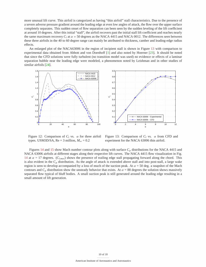
more unusual lift curve. This airfoil is categorized as having “thin airfoil” stall characteristics. Due to the presence ofa severe adverse pressure gradient around the leading edge at even low angles of attack, the flow over the upper surfacecompletely separates. This sudden onset of flow separation can been seen by the sudden leveling of the lift coefficientat around 10 degrees. After this initial “stall”, the airfoil recovers past the initial stall lift coefficient and reaches nearlythe same maximum recoveryCl atα = 50 degrees as the NACA 4415 and NACA 0012. The differences seen betweenthese three airfoils in the 40 to 60 degree range can mainly beattributed to thickness, camber and leading-edge radiuseffects.

An enlarged plot of the NACA63006 in the region of incipient stall is shown in Figure13 with comparison toexperimental data obtained from Abbott and von Doenhoff [1] and also noted by Hoerner [23]. It should be notedthat since the CFD solutions were fully turbulent (no transition model was used) no evidence or effects of a laminarseparation bubble near the leading edge were modeled, a phenomenon noted by Leishman and in other studies ofsimilar airfoils [24].

0 20 40 60 80 1000

0.2

0.4

0.6

0.8

1

1.2

1.4

1.6

1.8

α

Cl

NACA 4415NACA 0012NACA 63006

Figure 12: Comparison ofCl vs. α for three airfoiltypes. USM3D/SA, Re = 3 million,M∞ = 0.2

0 2 4 6 8 10 120

0.1

0.2

0.3

0.4

0.5

0.6

0.7

0.8

0.9

α

Cl

NACA 63006 − Experimental

NACA 63006 − CFD

Figure 13: Comparison ofCl vs. α from CFD andexperiment for the NACA 63006 thin airfoil.

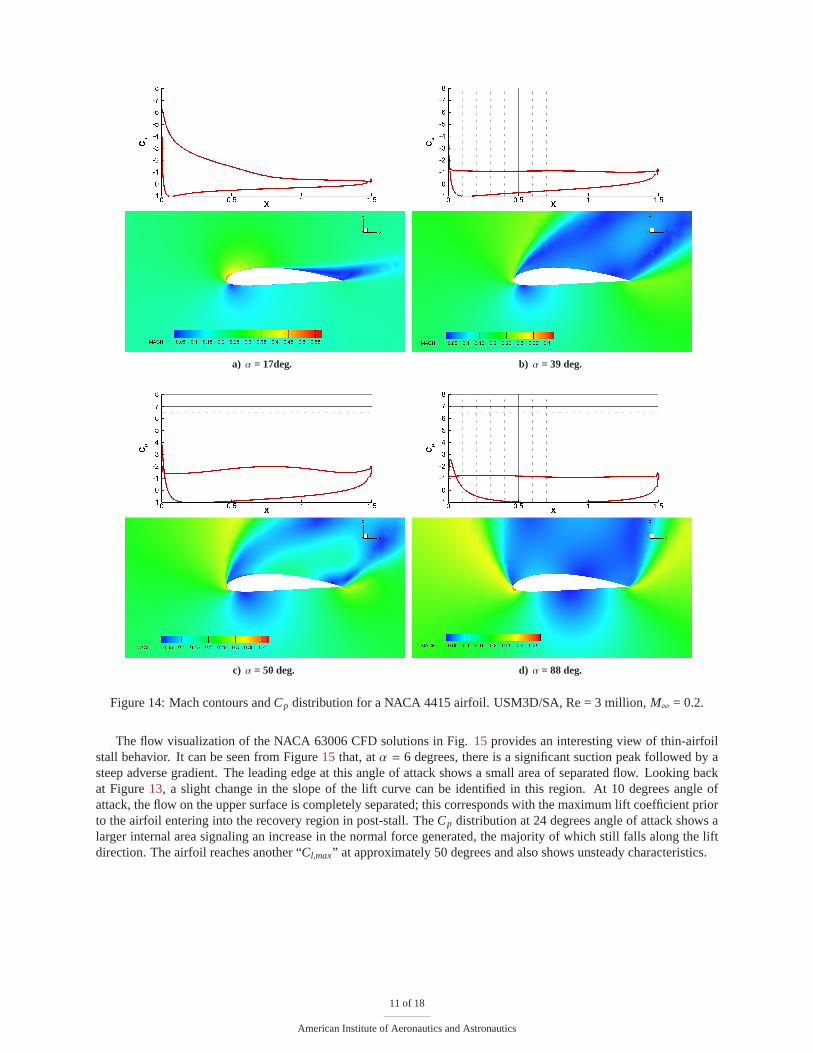
Figures14 and15 show Mach number contour plots along with surfaceCp distributions for the NACA 4415 andNACA 63006 airfoils at different stages along their respective lift curves. The NACA 4415 flow visualization in Fig.14 at α = 17 degrees. (Cl,max) shows the presence of trailing edge stall propagating forward along the chord. Thisis also evident in theCp distribution. As the angle of attack is extended above stalland into post-stall, a large wakeregion is seen to develop accompanied by a loss of much of the suction peak. Atα = 50 deg. a snapshot of the Machcontours andCp distribution show the unsteady behavior that exists. Atα = 88 degrees the solution shows massivelyseparated flow typical of bluff bodies. A small suction peak is still generated around the leading edge resulting in asmall amount of lift generation.

10 of 18

American Institute of Aeronautics and Astronautics

a) α = 17deg. b) α = 39 deg.

c) α = 50 deg. d) α = 88 deg.

Figure 14: Mach contours andCp distribution for a NACA 4415 airfoil. USM3D/SA, Re = 3 million, M∞ = 0.2.

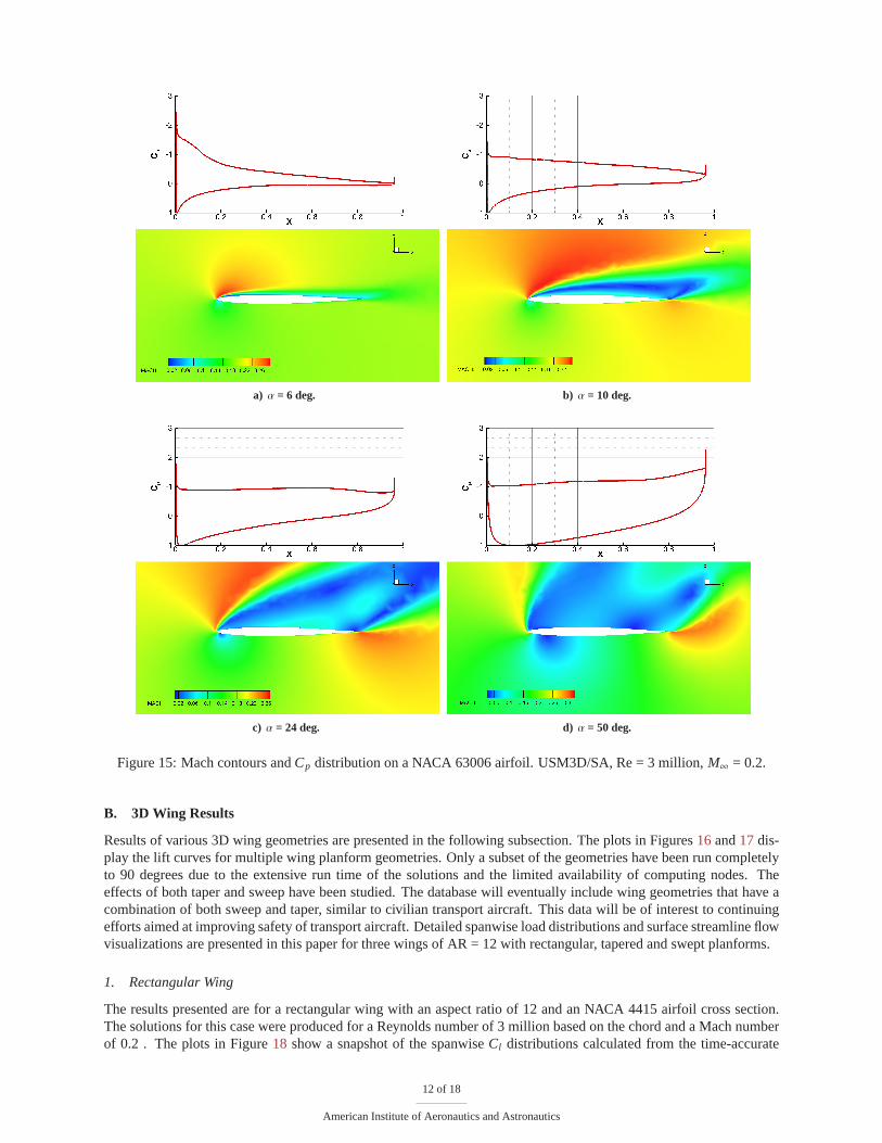
The flow visualization of the NACA 63006 CFD solutions in Fig.15 provides an interesting view of thin-airfoilstall behavior. It can be seen from Figure15 that, atα = 6 degrees, there is a significant suction peak followed by asteep adverse gradient. The leading edge at this angle of attack shows a small area of separated flow. Looking backat Figure13, a slight change in the slope of the lift curve can be identified in this region. At 10 degrees angle ofattack, the flow on the upper surface is completely separated; this corresponds with the maximum lift coefficient priorto the airfoil entering into the recovery region in post-stall. The Cp distribution at 24 degrees angle of attack shows alarger internal area signaling an increase in the normal force generated, the majority of which still falls along the liftdirection. The airfoil reaches another “Cl,max” at approximately 50 degrees and also shows unsteady characteristics.

11 of 18

American Institute of Aeronautics and Astronautics

a) α = 6 deg. b) α = 10 deg.

c) α = 24 deg. d) α = 50 deg.

Figure 15: Mach contours andCp distribution on a NACA 63006 airfoil. USM3D/SA, Re = 3 million, M∞ = 0.2.

B. 3D Wing Results

Results of various 3D wing geometries are presented in the following subsection. The plots in Figures16 and17 dis-play the lift curves for multiple wing planform geometries.Only a subset of the geometries have been run completelyto 90 degrees due to the extensive run time of the solutions and the limited availability of computing nodes. Theeffects of both taper and sweep have been studied. The database will eventually include wing geometries that have acombination of both sweep and taper, similar to civilian transport aircraft. This data will be of interest to continuingefforts aimed at improving safety of transport aircraft. Detailed spanwise load distributions and surface streamlineflowvisualizations are presented in this paper for three wings of AR = 12 with rectangular, tapered and swept planforms.

1. Rectangular Wing

The results presented are for a rectangular wing with an aspect ratio of 12 and an NACA 4415 airfoil cross section.The solutions for this case were produced for a Reynolds number of 3 million based on the chord and a Mach numberof 0.2 . The plots in Figure18 show a snapshot of the spanwiseCl distributions calculated from the time-accurate

12 of 18

American Institute of Aeronautics and Astronautics

0 20 40 60 80 1000

0.2

0.4

0.6

0.8

1

1.2

1.4

1.6

1.8

α

Cl

NACA4415 − 2D CFDRectangular AR12 − NACA4415Taper (T.R. 0.5) AR12 − NACA4415

Figure 16: Effect of taper on unswept wings:CL vs.α.USM3D/SA, Re = 3 million,M∞ = 0.2.

0 20 40 60 80 1000

0.2

0.4

0.6

0.8

1

1.2

1.4

1.6

1.8

α

Cl

NACA4415 − 2D CFD

0 deg. Sweep AR12 − NACA4415

10 deg. Sweep AR12 − NACA4415

20 deg. Sweep AR12 − NACA4415

30 deg. Sweep AR12 − NACA4415

Figure 17: Effect of sweep on constant-chord wings:CL vs.α. USM3D/SA, Re = 3 million,M∞ = 0.2

CFD solutions for angles of attack near stall and into post-stall. It is seen that at an angle of attack of 18 degrees,a sawtooth pattern in theCl distribution is present. The extent of this sawtooth pattern seems to grow at 22 degreesand 28 degrees. Correlating these load distributions with flow visualization at the same angles of attack enlightenedthe reason for the sawtooth patterns. Through the use of surface streamlines it can be seen in Figure19 that as theangle of attack increases, reversed flow is seen aft of the separation line and shows the presences of multiple stall cellsforming along the semi-span of the wing. This causes certainsections along the wing to have more attached flowthan others, generating the oscillations in the the local lift coefficients going from the root to the tip. This stall cellformation eventually dissipates as the flow over the upper surface becomes fully separated and the region of reversedflow reaches the leading edge of the wing as can be seen at 28 degrees. The streamlines in Figure19 seem to suggestthat even in high angle of attack situations the surface flow is still relatively in the chord-wise direction for the majorityof the semi-span. There are some variations near the bordersof stall cells and near the wing tip as would be expecteddue to the influence of the tip vortex.

0 0.2 0.4 0.6 0.8 10.6

0.8

1

1.2

1.4

1.6

1.8

Spanwise distance (2y/b)

Sec

tion

Cl

14 deg.18 deg.22 deg.28 deg.

a) Local Cl distribution at various angles of attack

0 5 10 15 20 25 30 35 40 450.2

0.4

0.6

0.8

1

1.2

1.4

1.6

1.8

α deg.

CL

b) Corresponding points onCL vs.α curve

Figure 18: Comparison of localCl distribution at various angles of attack for a rectangular wing AR = 12. USM3D/SA,Re = 3 million,M∞ = 0.2.

13 of 18

American Institute of Aeronautics and Astronautics

a) α = 14 deg. b) α = 18 deg.

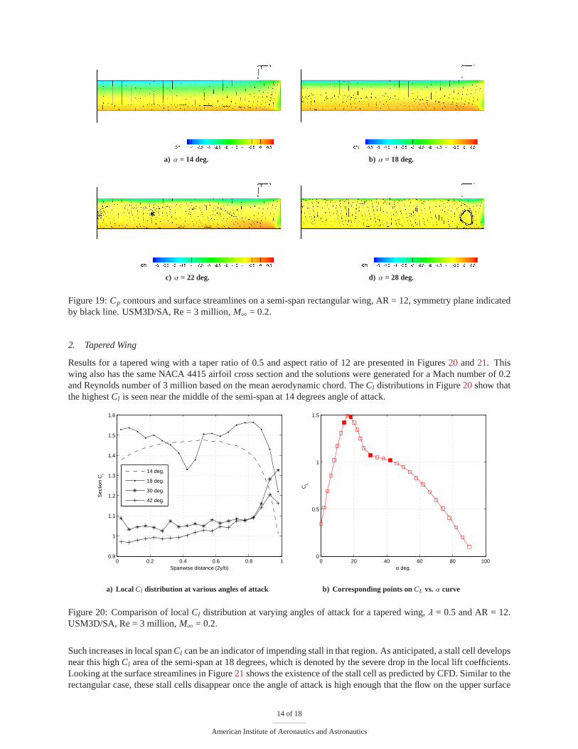
c) α = 22 deg. d) α = 28 deg.

Figure 19:Cp contours and surface streamlines on a semi-span rectangular wing, AR = 12, symmetry plane indicatedby black line. USM3D/SA, Re = 3 million,M∞ = 0.2.

2. Tapered Wing

Results for a tapered wing with a taper ratio of 0.5 and aspectratio of 12 are presented in Figures20 and21. Thiswing also has the same NACA 4415 airfoil cross section and thesolutions were generated for a Mach number of 0.2and Reynolds number of 3 million based on the mean aerodynamic chord. TheCl distributions in Figure20show thatthe highestCl is seen near the middle of the semi-span at 14 degrees angle ofattack.

0 0.2 0.4 0.6 0.8 10.9

1

1.1

1.2

1.3

1.4

1.5

1.6

Spanwise distance (2y/b)

Sec

tion

Cl

14 deg.

18 deg.

30 deg.

42 deg.

a) Local Cl distribution at various angles of attack

0 20 40 60 80 1000

0.5

1

1.5

α deg.

CL

b) Corresponding points onCL vs.α curve

Figure 20: Comparison of localCl distribution at varying angles of attack for a tapered wing,λ = 0.5 and AR = 12.USM3D/SA, Re = 3 million,M∞ = 0.2.

Such increases in local spanCl can be an indicator of impending stall in that region. As anticipated, a stall cell developsnear this highCl area of the semi-span at 18 degrees, which is denoted by the severe drop in the local lift coefficients.Looking at the surface streamlines in Figure21shows the existence of the stall cell as predicted by CFD. Similar to therectangular case, these stall cells disappear once the angle of attack is high enough that the flow on the upper surface

14 of 18

American Institute of Aeronautics and Astronautics

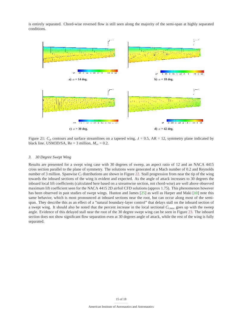
is entirely separated. Chord-wise reversed flow is still seen along the majority of the semi-span at highly separatedconditions.

a) α = 14 deg. b) α = 18 deg.

c) α = 30 deg. d) α = 42 deg.

Figure 21:Cp contours and surface streamlines on a tapered wing,λ = 0.5, AR = 12, symmetry plane indicated byblack line. USM3D/SA, Re = 3 million,M∞ = 0.2.

3. 30 Degree Swept Wing

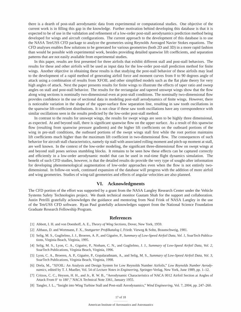
Results are presented for a swept wing case with 30 degrees ofsweep, an aspect ratio of 12 and an NACA 4415cross section parallel to the plane of symmetry. The solutions were generated at a Mach number of 0.2 and Reynoldsnumber of 3 million. SpanwiseCl distributions are shown in Figure22. Stall progression from near the tip of the wingtowards the inboard sections of the wing is evident and expected. As the angle of attack increases to 30 degrees theinboard local lift coefficients (calculated here based on a streamwise section, not chord-wise) are well above observedmaximum lift coefficient seen for the NACA 4415 2D airfoil CFDsolutions (approx 1.75). This phenomenon howeverhas been observed in past studies of swept wings. Hunton and James [25] as well as Harper and Maki [10] note thissame behavior, which is most pronounced at inboard sectionsnear the root, but can occur along most of the semi-span. They describe this as an effect of a ”natural boundary-layer control” that delays stall on the inboard section ofa swept wing. It should also be noted that the percent increase in the local sectionalCl,max goes up with the sweepangle. Evidence of this delayed stall near the root of the 30 degree swept wing can be seen in Figure23. The inboardsection does not show significant flow separation even at 30 degrees angle of attack, while the rest of the wing is fullyseparated.

15 of 18

American Institute of Aeronautics and Astronautics

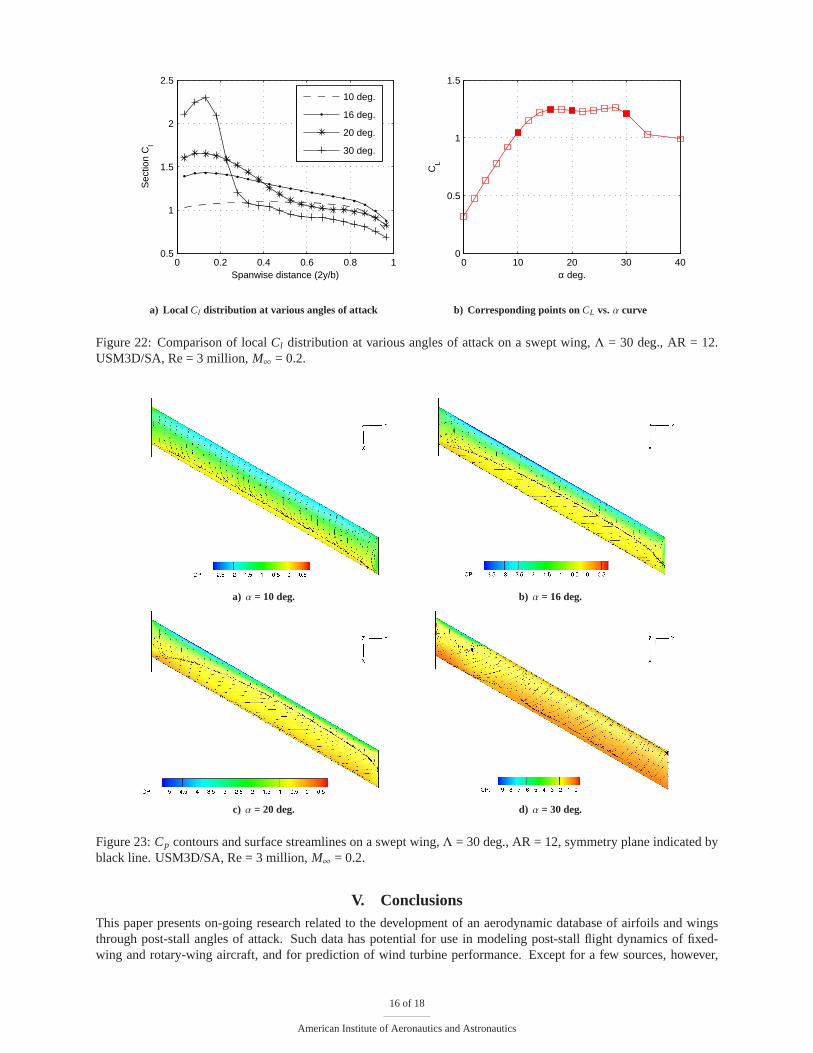
0 0.2 0.4 0.6 0.8 10.5

1

1.5

2

2.5

Spanwise distance (2y/b)

Sec

tion

Cl

10 deg.

16 deg.

20 deg.

30 deg.

a) Local Cl distribution at various angles of attack

0 10 20 30 400

0.5

1

1.5

α deg.

CL

b) Corresponding points onCL vs.α curve

Figure 22: Comparison of localCl distribution at various angles of attack on a swept wing,Λ = 30 deg., AR = 12.USM3D/SA, Re = 3 million,M∞ = 0.2.

a) α = 10 deg. b) α = 16 deg.

c) α = 20 deg. d) α = 30 deg.

Figure 23:Cp contours and surface streamlines on a swept wing,Λ = 30 deg., AR = 12, symmetry plane indicated byblack line. USM3D/SA, Re = 3 million,M∞ = 0.2.

V. ConclusionsThis paper presents on-going research related to the development of an aerodynamic database of airfoils and wingsthrough post-stall angles of attack. Such data has potential for use in modeling post-stall flight dynamics of fixed-wing and rotary-wing aircraft, and for prediction of wind turbine performance. Except for a few sources, however,

16 of 18

American Institute of Aeronautics and Astronautics

there is a dearth of post-stall aerodynamic data from experimental or computational studies. One objective of thecurrent work is in filling this gap in the knowledge. Further motivation behind developing this database is that it isexpected to be of use in the validation and refinement of a low-order post-stall aerodynamics prediction method beingdeveloped for wings and aircraft configurations. The current approach to the development of this database is to usethe NASA TetrUSS CFD package to analyze the geometries usingReynolds Averaged Navier Stokes equations. TheCFD analyses enables flow solutions to be generated for various geometries (both 2D and 3D) in a more rapid fashionthan would be possible with experimental work, besides providing detailed spanwise lift coefficients, and separationpatterns that are not easily available from experimental studies.

In this paper, results are first presented for three airfoilsthat exhibit different stall and post-stall behaviors. Theresults for these and other airfoils will be used as input data for the low-order post-stall prediction method for finitewings. Another objective in obtaining these results is thatstudying the post-stall behavior of these airfoils may leadto the development of a rapid method of generating airfoil force and moment curves from 0 to 90 degrees angle ofattack using a combination of results from XFOIL and other simplified models such as the flat plate theory for veryhigh angles of attack. Next the paper presents results for finite wings to illustrate the effects of taper ratio and sweepangles on stall and post-stall behavior. The results for therectangular and tapered unswept wings show that the flowalong wing sections is nominally two-dimensional even at post-stall conditions. The nominally two-dimensional flowprovides confidence in the use of sectional data in modeling post-stall aerodynamics of finite wings. However, thereis noticeable variation in the shape of the upper-surface flow separation line, resulting in saw tooth oscillations inthe spanwise lift-coefficient distributions. It is not clear if these saw tooth oscillations have any correspondence withsimilar oscillations seen in the results predicted by the low-order post-stall method.

In contrast to the results for unswept wings, the results forswept wings are seen to be highly three dimensional,as expected. At and beyond stall, there is significant spanwise flow on the upper surface. As a result of this spanwiseflow (resulting from spanwise pressure gradients) and the higher lift coefficients on the outboard portions of thewing in pre-stall conditions, the outboard portions of the swept wings stall first while the root portion maintainslift coefficients much higher than the maximum lift coefficient in two-dimensional flow. The consequences of suchbehavior for aircraft stall characteristics, namely tip stall with associated rolling moment and pitch-up moment at stall,are well known. In the context of the low-order modeling, thesignificant three-dimensional flow on swept wings atand beyond stall poses serious stumbling blocks. It remainsto be seen how these effects can be captured correctlyand efficiently in a low-order aerodynamic model that can be used in real-time flight dynamics simulation. Thebenefit of such CFD studies, however, is that the detailed results do provide the very type of sought-after informationfor developing phenomenological augmentation of low-order approaches even when the flow is not entirely two-dimensional. In follow-on work, continued expansion of thedatabase will progress with the addition of more airfoiland wing geometries. Studies of wing-tail geometries and effects of angular velocities are also planned.

VI. AcknowledgmentsThe CFD portion of the effort was supported by a grant from theNASA Langley Research Center under the VehicleSystems Safety Technologies project. We thank technical monitor Gautam Shah for the support and collaboration.Justin Petrilli gratefully acknowledges the guidance and mentoring from Neal Frink of NASA Langley in the useof the TetrUSS CFD software. Ryan Paul gratefully acknowledges support from the National Science FoundationGraduate Research Fellowship Program.

References[1] Abbott, I. H. and von Doenhoff, A. E.,Theory of Wing Sections, Dover, New York, 1959.

[2] Althaus, D. and Wortmann, F. X.,Stuttgarter Profilkatalog I, Friedr. Vieweg & Sohn, Braunschweig, 1981.

[3] Selig, M. S., Guglielmo, J. J., Broeren, A. P., and Giguere, P.,Summary of Low-Speed Airfoil Data, Vol. 1, SoarTech Publica-tions, Virginia Beach, Virginia, 1995.

[4] Selig, M. S., Lyon, C. A., Giguere, P., Ninham, C. N., and Guglielmo, J. J.,Summary of Low-Speed Airfoil Data, Vol. 2,SoarTech Publications, Virginia Beach, Virginia, 1996.

[5] Lyon, C. A., Broeren, A. P., Giguere, P., Gopalarathnam, A., and Selig, M. S.,Summary of Low-Speed Airfoil Data, Vol. 3,SoarTech Publications, Virginia Beach, Virginia, 1998.

[6] Drela, M., “XFOIL: An Analysis and Design System for Low Reynolds Number Airfoils,”Low Reynolds Number Aerody-namics, edited by T. J. Mueller, Vol. 54 ofLecture Notes in Engineering, Springer-Verlag, New York, June 1989, pp. 1–12.

[7] Critzos, C. C., Heyson, H. H., and Jr., R. W. B., “AerodynamicCharacteristics of NACA 0012 Airfoil Section at Angles ofAttack From 0◦ to 180◦,” NACA Technical Note 3361, January 1955.

[8] Tangler, J. L., “Insight into Wing Turbine Stall and Post-stall Aerodynamics,”Wind Engineering, Vol. 7, 2004, pp. 247–260.

17 of 18

American Institute of Aeronautics and Astronautics

[9] Lindenburg, C., “Aerodynamic Airfoil Coefficients at Large Angles of Attack,” IEA Symposium Paper ECN-RX–01-004,2001.

[10] Harper, C. W. and Maki, R. L., “A Review of the Stall Characteristics of Swept Wings,” NASA TN D-2373, 1964.

[11] Ostowari, C. and Naik, D., “Post Stall Studies of Untwisted Varying Aspect Ratio Blades with an NACA 4415 AirfoilSection—Part 1,”Wind Engineering, Vol. 8, No. 3, 1984, pp. 176–194.

[12] Mukherjee, R. and Gopalarathnam, A., “Poststall Prediction of Multiple-Lifting-Surface Configurations Using a DecamberingApproach,”Journal of Aircraft, Vol. 43, No. 3, May–June 2006, pp. 660–668.

[13] Gopalarathnam, A., Paul, R., and Petrilli, J., “Aerodynamic Modeling for Real-Time Flight Dynamics Simulation (Invited),”AIAA Paper 2013-0969, January 2013.

[14] Frink, N. T., Pirzadeh, S., Parikh, P., and Pandya, M., “TheNASA Tetrahedral Unstructured Software System (TetrUSS),”The Aeronautical Journal, Vol. 104, No. 1040, 2000, pp. 491–499.

[15] Pirzadeh, S., “Three-Dimensional Unstructured Grids by the Advancing Layer Method,”AIAA Journal, Vol. 33, No. 1, 1996,pp. 43–49.

[16] Pirzadeh, S., “Unstructured Viscous Grid Generation by the Advancing-Layers Method,”AIAA Journal, Vol. 32, No. 8, 1994,pp. 1735–1737.

[17] Lohner, R. and Parikh, P., “Three-dimensional grid generation by the advancing front method,”International Journal forNumerical Methods in Fluids, Vol. 8, No. 10, 1988, pp. 1135–1149.

[18] Frink, N. T., “Tetrahedral Unstructured Navier-Stokes Methodfor Turbulent Flows,”AIAA Journal, Vol. 36, No. 11, 1998,pp. 1975–1982.

[19] Fredericks, W. J., Antcliff, K. R., Costa, G., Deshpande, N.,Moore, M. D., Miguel, E. A. S., and Snyder, A. N., “AircraftConceptual Design Using Vehicle Sketch Pad,” AIAA Paper 2010-658,2010.

[20] Frink, N. T., Pirzadeh, S. Z., Atkins, H. L., Viken, S. A., and Morrison, J. H., “CFD Assessment of Aerodynamic Degradationof Subsonic Transport Due to Airframe Damage,” AIAA Paper 2010-500, 2010.

[21] Spalart, P. and Allmaras, S., “One-Equation Turbulence Model for Aerodynamic Flows,” AIAA Paper 92-0429, 1992.

[22] Pandya, M. J., Khaled S. Abdol-Hamid, R. L. C., and Frink, N. T., “Implementation of Flow Tripping Capability in theUSM3D Unstructured Flow Solver,”AIAA Journal, , No. 2006-0919, January 2006.

[23] Hoerner, S. and Borst, H.,Fluid-Dynamic Lift, Hoerner Fluid Dynamics, 1985.

[24] Li, D., “Numerical Simulation of Thin Airfoil Stall By Using a Modified DES Approach,”International Journal For Numer-ical Methods In Fluid, Vol. 54, 2007, pp. 325–332.

[25] Hunton, L. W. and James, H. A., “Use of Two-Dimensional Data In Estimating Loads on a 45o Sweptback Wing with Slatsand Partial-Span Flaps,” NACA TN 3040, 1953.

18 of 18

American Institute of Aeronautics and Astronautics