A causal framework for explaining the predictions ofblack-box sequence-to-sequence models

David Alvarez-Melis and Tommi S. JaakkolaCSAIL, MIT

davidam, tommi@csail.mit.edu

Abstract

We interpret the predictions of any black-box structured input-structured outputmodel around a specific input-output pair.Our method returns an “explanation” con-sisting of groups of input-output tokensthat are causally related. The method in-fers these dependencies by querying themodel with perturbed inputs, generatinga graph over tokens from the responses,and solving a partitioning problem to se-lect the most relevant components. We fo-cus the general approach on sequence-to-sequence problems, adopting a variationalautoencoder to yield meaningful input per-turbations. We test our method across sev-eral NLP sequence generation tasks.

1 Introduction

Interpretability is often the first casualty whenadopting complex predictors. This is particularlytrue for structured prediction methods at the coreof many natural language processing tasks suchas machine translation (MT). For example, deeplearning models for NLP involve a large num-ber of parameters and complex architectures, mak-ing them practically black-box systems. Whilesuch systems achieve state-of-the-art results inMT (Bahdanau et al., 2014), summarization (Rushet al., 2015) and speech recognition (Chan et al.,2015), they remain largely uninterpretable, al-though attention mechanisms (Bahdanau et al.,2014) can shed some light on how they operate.

Stronger forms of interpretability could offerseveral advantages, from trust in model predic-

tions, error analysis, to model refinement. Forexample, critical medical decisions are increas-ingly being assisted by complex predictions thatshould lend themselves to easy verification by hu-man experts. Without understanding how inputsget mapped to the outputs, it is also challenging todiagnose the source of potential errors. A slightlyless obvious application concerns model improve-ment (Ribeiro et al., 2016) where interpretabilitycan be used to detect biases in the methods.

Interpretability has been approached primarilyfrom two main angles: model interpretability, i.e.,making the architecture itself interpretable, andprediction interpretability, i.e., explaining particu-lar predictions of the model (cf. (Lei et al., 2016)).Requiring the model itself to be transparent is of-ten too restrictive and challenging to achieve. In-deed, prediction interpretability can be more eas-ily sought a posteriori for black-box systems in-cluding neural networks.

In this work, we propose a novel approach toprediction interpretability with only oracle accessto the model generating the prediction. Following(Ribeiro et al., 2016), we turn the local behaviorof the model around the given input into an inter-pretable representation of its operation. In con-trast to previous approaches, we consider struc-tured prediction where both inputs and outputs arecombinatorial objects, and our explanation con-sists of a summary of operation rather than a sim-pler prediction method.

Our method returns an “explanation” consistingof sets of input and output tokens that are causallyrelated under the black-box model. Causal de-pendencies arise from analyzing perturbed ver-sions of inputs that are passed through the black-

box model. Although such perturbations might beavailable in limited cases, we generate them auto-matically. For sentences, we adopt a variationalautoencoder to produce semantically related sen-tence variations. The resulting inferred causal de-pendencies (interval estimates) form a dense bi-partite graph over tokens from which explanationscan be derived as robust min-cut k-partitions.

We demonstrate quantitatively that our methodcan recover known dependencies. As a startingpoint, we show that a grapheme-to-phoneme dic-tionary can be largely recovered if given to themethod as a black-box model. We then show thatthe explanations provided by our method closelyresemble the attention scores used by a neural ma-chine translation system. Moreover, we illustratehow our summaries can be used to gain insightsand detect biases in translation systems. Our maincontributions are:

• We propose a general framework for explain-ing structured black-box models

• For sequential data, we propose a variationalautoencoder for controlled generation of in-put perturbations required for causal analysis

• We evaluate the explanations produced byour framework on various sequence-to-sequence prediction tasks, showing they canrecover known associations and provide in-sights into the workings of complex systems.

2 Related Work

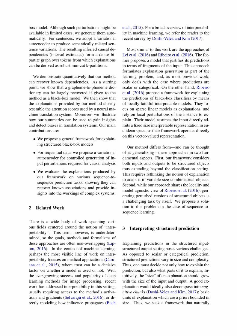
There is a wide body of work spanning vari-ous fields centered around the notion of “inter-pretability”. This term, however, is underdeter-mined, so the goals, methods and formalisms ofthese approaches are often non-overlapping (Lip-ton, 2016). In the context of machine learning,perhaps the most visible line of work on inter-pretability focuses on medical applications (Caru-ana et al., 2015), where trust can be a decisivefactor on whether a model is used or not. Withthe ever-growing success and popularity of deeplearning methods for image processing, recentwork has addressed interpretability in this setting,usually requiring access to the method’s activa-tions and gradients (Selvaraju et al., 2016), or di-rectly modeling how influence propagates (Bach

et al., 2015). For a broad overview of interpretabil-ity in machine learning, we refer the reader to therecent survey by Doshi-Velez and Kim (2017).

Most similar to this work are the approaches ofLei et al. (2016) and Ribeiro et al. (2016). The for-mer proposes a model that justifies its predictionsin terms of fragments of the input. This approachformulates explanation generation as part of thelearning problem, and, as most previous work,only deals with the case where predictions arescalar or categorical. On the other hand, Ribeiroet al. (2016) propose a framework for explainingthe predictions of black-box classifiers by meansof locally-faithful interpretable models. They fo-cus on sparse linear models as explanations, andrely on local perturbations of the instance to ex-plain. Their model assumes the input directly ad-mits a fixed size interpretable representation in eu-clidean space, so their framework operates directlyon this vector-valued representation.

Our method differs from—and can be thoughtof as generalizing—these approaches in two fun-damental aspects. First, our framework considersboth inputs and outputs to be structured objectsthus extending beyond the classification setting.This requires rethinking the notion of explanationto adapt it to variable-size combinatorial objects.Second, while our approach shares the locality andmodel-agnostic view of Ribeiro et al. (2016), gen-erating perturbed versions of structured objects isa challenging task by itself. We propose a solu-tion to this problem in the case of sequence-to-sequence learning.

3 Interpreting structured prediction

Explaining predictions in the structured input-structured output setting poses various challenges.As opposed to scalar or categorical prediction,structured predictions vary in size and complexity.Thus, one must decide not only how to explain theprediction, but also what parts of it to explain. In-tuitively, the “size” of an explanation should growwith the size of the input and output. A good ex-planation would ideally also decompose into cog-nitive chunks (Doshi-Velez and Kim, 2017): basicunits of explanation which are a priori bounded insize. Thus, we seek a framework that naturally

decomposes an explanation into (potentially sev-eral) explaining components, each of which justi-fies, from the perspective of the black-box model,parts of the output relative to the parts of the input.

Formally, suppose we have a black-box modelF : X → Y that maps a structured input x ∈ Xto a structured output y ∈ Y . We make no as-sumptions on the spaces X ,Y , except that theirelements admit a feature-set representation x =x1, x2, . . . , xn, y = y1, y2, . . . , ym. Thus, xand y can be sequences, graphs or images. Werefer to the elements xi and yj as units or “to-kens” due to our motivating application of sen-tences, though everything in this work holds forother combinatorial objects.

For a given input output pair (x,y), we are in-terested in obtaining an explanation of y in termsof x. Following (Ribeiro et al., 2016), we seekexplanations via interpretable representations thatare both i) locally faithful, in the sense that theyapproximate how the model behaves in the vicinityof x, and ii) model agnostic, that is, that do not re-quire any knowledge ofF . For example, we wouldlike to identify whether token xi is a likely causefor the occurrence of yj in the output when the in-put context is x. Our assumption is that we cansummarize the behavior of F around x in termsof a weighted bipartite graph G = (Vx ∪ Vy, E),where the nodes Vx and Vy correspond to the el-ements in x and y, respectively, and the weightof each edge Eij corresponds to the influence ofthe occurrence of token xi on the appearance ofyj . The bipartite graph representation suggestsnaturally that the explanation be given in terms ofexplaining components. We can formalize thesecomponents as subgraphs Gk = (V k

x ∪ V ky , E

k),where the elements in V k

x are likely causes forthe elements in V k

y . Thus, we define an expla-nation of y as a collection of such components:Ex→y = G1, . . . , Gk.

Our approach formalizes this frameworkthrough a pipeline (sketched in Figure 1) consist-ing of three main components, described in detailin the following section: a perturbation model forexercising F locally, a causal inference modelfor inferring associations between inputs and pre-dictions, and a selection step for partitioning andselecting the most relevant sets of associations.

We refer to this framework as a structured-outputcausal rationalizer (SOCRAT).

A note on alignment models When the inputsand outputs are sequences such as sentences, onemight envision using an alignment model, suchas those used in MT, to provide an explanation.This differs from our approach in several respects.Specifically, we focus on explaining the behaviorof the “black box” mapping F only locally, aroundthe current input context, not globally. Any globalalignment model would require access to substan-tial parallel data to train and would have vary-ing coverage of the local context around the spe-cific example of interest. Any global model wouldlikely also suffer from misspecification in relationto F . A more related approach to ours would bean alignment model trained locally based on thesame perturbed sentences and associated outputsthat we generate.

4 Building blocks

4.1 Perturbation Model

The first step in our approach consists of obtain-ing perturbed versions of the input: semanticallysimilar to the original but with potential changes inelements and their order. This is a major challengewith any structured inputs. We propose to do thisusing a variational autoencoder (VAE) (Kingmaand Welling, 2014; Rezende et al., 2014). VAEshave been successfully used with fixed dimen-sional inputs such as images (Rezende and Mo-hamed, 2015; Sønderby et al., 2016) and recentlyalso adapted to generating sentences from contin-uous representations (Bowman et al., 2016). Thegoal is to introduce the perturbation in the contin-uous latent representation rather than directly onthe structured inputs.

A VAE is composed of a probabilistic encoderENC : X → Rd and a decoder DEC : Rd →X . The encoder defines a distribution over la-tent codes q(z|x), typically by means of a two-step procedure that first maps x 7→ (µ,σ) andthen samples z from a gaussian distribution withthese parameters. We can leverage this stochas-ticity to obtain perturbed versions of the input

PerturbationModel

CausalInference

ExplanationSelection

(x,y) (xi, yi) G(U ∪ V,E) Ekx→yKk=1

z

z1

z2z3

z4

z5z6

z7

z8 s1 s2 s3 s4

t1 t2 t3 t4 t5

s1 s2

t1 t2 t3

s1 s2

t1 t2

Figure 1: A schematic representation of the proposed prediction interpretability method.

by sampling repeatedly from this distribution, andthen mapping these back to the original space us-ing the decoder. The training regime for the VAEensures approximately that a small perturbationof the hidden representation maintains similar se-mantic content while introducing small changes inthe decoded surface form. We emphasize that theapproach would likely fail with an ordinary au-toencoder where small changes in the latent rep-resentation can result in large changes in the de-coded output. In practice, we ensure diversity ofperturbations by scaling the variance term σ andsampling points z and different resolutions. Weprovide further details of this procedure in the sup-plement. Naturally, we can train this perturba-tion model in advance on (unlabeled) data fromthe input domain X , and then use it as a subrou-tine in our method. After this process is com-plete, we have N pairs of perturbed input-outputpairs: (xi, yi)Ni=1 which exercise the mappingF around semantically similar inputs.

4.2 Causal model

The second step consists of using the perturbedinput-output pairs (xi, yi)Ni=1 to infer causal de-pendencies between the original input and outputtokens. A naive approach would consider 2x2 con-tingency tables representing presence/absence ofinput/output tokens together with a test statistic forassessing their dependence. Instead, we incorpo-rate all input tokens simultaneously to predict theoccurrence of a single output token via logistic re-gression. The quality of these dependency estima-tors will depend on the frequency with which eachinput and output token occurs in the perturbations.Thus, we are interested in obtaining uncertaintyestimates for these predictions, which can be nat-urally done with a Bayesian approach to logisticregression. Let φx(x) ∈ 0, 1|x| be a binary vec-tor encoding the presence of the original tokens

x1, . . . , xn from x in the perturbed version x. Foreach target token yj ∈ y, we estimate a model:

P (yj ∈ y | x) = σ(θTj φx(x)) (1)

where σ(z) = (1 + exp(−z))−1. We use a Gaus-sian approximation for the logarithm of the lo-gistic function together with the prior p(θ) =N (θ0,H

−10 ) (Murphy, 2012). Since in our case all

tokens are guaranteed to occur at least once (we in-clude the original example pair as part of the set),we use θ0 = α1,H0 = βI, with α, β > 0. Uponcompletion of this step, we have dependency co-efficients between all original input and output to-kens θij, along with their uncertainty estimates.

4.3 Explanation Selection

The last step in our interpretability frameworkconsists of selecting a set explanations for (x,y).The steps so far yield a dense bipartite graph be-tween the input and output tokens. Unless |x| and|y| are small, this graph itself may not be suf-ficiently interpretable. We are interested in se-lecting relevant components of this dependencygraph, i.e., partition the vertex set of G into dis-joint subsets so as to minimize the weight of omit-ted edges (i.e. the k-cut value of the partition).

Graph partitioning is a well studied NP-complete problem (Garey et al., 1976). The usualsetting assumes deterministic edge weights, but inour case we are interested in incorporating the un-certainty of the dependency estimates—resultingfrom their finite sample estimation—into the par-titioning problem. For this, we rely on the ap-proach of Fan et al. (2012) designed for intervalestimates of edge weights. At a high level, this isa robust optimization formulation which seeks tominimize worst case cut values, and can be castas a Mixed Integer Programming (MIP) problem.Specifically, for a bipartite graph G = (U, V,E)

Algorithm 1 Structured-output causal rationalizer1: procedure SOCRAT(x,y, F )2: (µ,σ)← ENCODE(x)3: for i = 1 to N do4: zi ← SAMPLE(µ,σ)

PerturbationModel.5: xi ← DECODE(zi)

6: yi ← F (xi)7: end for8: G ← CAUSAL(x,y, xi, yiNi=1)9: Ex 7→y ← BIPARTITION(G)

10: Ex 7→y ← SORT(Ex 7→y) . By cut capacity11: return Ex7→y

12: end procedure

with edge weights given as uncertainty intervalsθij ± θij , the partitioning problem is given by

min(xu

ik,xvjk,yij)∈Y

n∑i=1

m∑j=1

θijyij+

maxS:S⊆V,|S|≤Γ(it,jt)∈V \S

∑(i,j)∈S

θijyij + (Γ− bΓc)θit,jtyit,jt

(2)

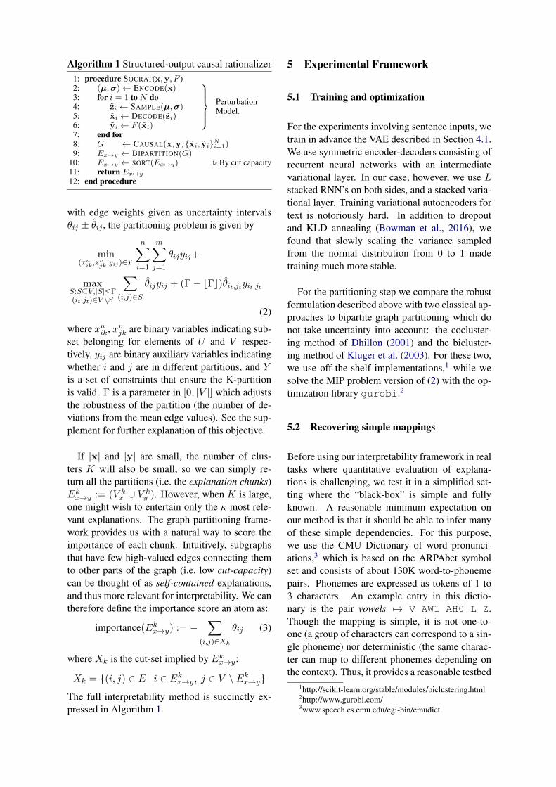
where xuik, xvjk are binary variables indicating sub-set belonging for elements of U and V respec-tively, yij are binary auxiliary variables indicatingwhether i and j are in different partitions, and Yis a set of constraints that ensure the K-partitionis valid. Γ is a parameter in [0, |V |] which adjuststhe robustness of the partition (the number of de-viations from the mean edge values). See the sup-plement for further explanation of this objective.

If |x| and |y| are small, the number of clus-ters K will also be small, so we can simply re-turn all the partitions (i.e. the explanation chunks)Ek

x→y := (V kx ∪ V k

y ). However, when K is large,one might wish to entertain only the κ most rele-vant explanations. The graph partitioning frame-work provides us with a natural way to score theimportance of each chunk. Intuitively, subgraphsthat have few high-valued edges connecting themto other parts of the graph (i.e. low cut-capacity)can be thought of as self-contained explanations,and thus more relevant for interpretability. We cantherefore define the importance score an atom as:

importance(Ekx→y) := −

∑(i,j)∈Xk

θij (3)

where Xk is the cut-set implied by Ekx→y:

Xk = (i, j) ∈ E | i ∈ Ekx→y, j ∈ V \ Ek

x→yThe full interpretability method is succinctly ex-pressed in Algorithm 1.

5 Experimental Framework

5.1 Training and optimization

For the experiments involving sentence inputs, wetrain in advance the VAE described in Section 4.1.We use symmetric encoder-decoders consisting ofrecurrent neural networks with an intermediatevariational layer. In our case, however, we use Lstacked RNN’s on both sides, and a stacked varia-tional layer. Training variational autoencoders fortext is notoriously hard. In addition to dropoutand KLD annealing (Bowman et al., 2016), wefound that slowly scaling the variance sampledfrom the normal distribution from 0 to 1 madetraining much more stable.

For the partitioning step we compare the robustformulation described above with two classical ap-proaches to bipartite graph partitioning which donot take uncertainty into account: the cocluster-ing method of Dhillon (2001) and the bicluster-ing method of Kluger et al. (2003). For these two,we use off-the-shelf implementations,1 while wesolve the MIP problem version of (2) with the op-timization library gurobi.2

5.2 Recovering simple mappings

Before using our interpretability framework in realtasks where quantitative evaluation of explana-tions is challenging, we test it in a simplified set-ting where the “black-box” is simple and fullyknown. A reasonable minimum expectation onour method is that it should be able to infer manyof these simple dependencies. For this purpose,we use the CMU Dictionary of word pronunci-ations,3 which is based on the ARPAbet symbolset and consists of about 130K word-to-phonemepairs. Phonemes are expressed as tokens of 1 to3 characters. An example entry in this dictio-nary is the pair vowels 7→ V AW1 AH0 L Z.Though the mapping is simple, it is not one-to-one (a group of characters can correspond to a sin-gle phoneme) nor deterministic (the same charac-ter can map to different phonemes depending onthe context). Thus, it provides a reasonable testbed

1http://scikit-learn.org/stable/modules/biclustering.html2http://www.gurobi.com/3www.speech.cs.cmu.edu/cgi-bin/cmudict

20 40 60 80 100Samples

0.50

0.55

0.60

0.65

0.70

0.75

0.80

0.85A

ER

Align - Full Vocab

20 40 60 80 100Samples

0.3

0.4

0.5

0.6

0.7

0.8

0.9

1.0

F1

Align - Full Vocab

Uncertainty Biclustering Coclustering Alignment

Figure 2: Arpabet test results as a function of num-ber of perturbations used. Shown are mean plusconfidence bounds over 5 repetitions. Left: Align-ment Error Rate, Right: F1 over edge prediction.

for our method. The setting is as follows: given aninput-output pair from the cmudict “black-box”,we use our method to infer dependencies betweencharacters in the input and phonemes in the out-put. Since locality in this context is morphologi-cal instead of semantic, we produce perturbationsselecting n words randomly from the intersectionof the cmudict vocabulary and the set of wordswith edit distance at most 2 from the original word.

To evaluate the inferred dependencies, we ran-domly selected 100 key-value pairs from the dic-tionary and manually labeled them with character-to-phoneme alignments. Even though our frame-work is not geared to produce pairwise align-ments, it should nevertheless be able to recoverthem to a certain extent. To provide a point ofreference, we compare against a (strong) base-line that is tailored to such a task: a state-of-the-art unsupervised word alignment method based onMonte Carlo inference (Tiedemann and Östling,2016). The results in Figure 2 show that theversion of our method that uses the uncertaintyclustering performs remarkably close to the align-ment system, with an alignment error rate only tenpoints above an oracle version of this system thatwas trained on the full arpabet dictionary (dashedline). The raw and partitioned explanations pro-vided by our method for an example input-outputpair are shown in Table 1, where the edge widthscorrespond to the estimated strength of depen-dency. Throughout this work we display the nodesin the same lexical order of the inputs/outputs tofacilitate reading, even if that makes the explana-tion chunks less visibly discernible. Instead, wesometimes provide an additional (sorted) heatplot

Raw Dependencies Explanation Graph

ob no a

UW0

l e

IY1 AH0B NL

→ob no a

UW0

l e

IY1 AH0B NL

ob no a

UW0

l e

IY1 AH0B NL

→ob no a

UW0

l e

IY1 AH0B NL

Table 1: Inferred dependency graphs before (left)and after (right) explanation selection for the pre-diction: boolean 7→ B UW0 L IY1 AH0 N, inindependent runs with large (top) and small (bot-tom) clustering parameter k.

of dependency values to show these partitions.

5.3 Machine Translation

In our second set of experiments we evaluateour explanation model in a relevant and popularsequence-to-sequence task: machine translation.As black-boxes, we use three different methods fortranslating English into German: (i) Azure’s Ma-chine Translation system, (ii) a Neural MT model,and (iii) a human (native speaker of German). Weprovide details on all three systems in the supple-ment. We translate the same English sentenceswith all three methods, and explain their predic-tions using SOCRAT. To be able to generate sen-tences with similar language and structure as thoseused to train the two automatic systems, we use themonolingual English side of the WMT14 datasetto train the variational autoencoder described inSection 4.1. For every explanation instance, wesample S = 100 perturbations and use the black-boxes to translate them. In all cases, we use thesame default SOCRAT configurations, includingthe robust partitioning method.

In Figure 3, we show the explanations providedby our method for the predictions of each of thethree systems on the input sentence “Students saidthey looked forward to his class”. Although thethree black-boxes all provided different transla-tions, the explanations show a mostly consistentclustering around the two phrases in the sentence,and in all three cases the cluster with the highestcut value (i.e. the most relevant explanative chunk)is the one containing the subject. Interestingly, the

Studenten

sagten,

dass sie

nach

vorne

Klasse

aussah. in

seine

.histoclassfor

wardloo

kedthe

ysaid

Studen

ts

class

sagten,

looked

dass

forwardtheysaid

vorne Klasseinsie seine

to

aussah.nachStudenten

.Students his

Studenten

sagten ,sie

dass auf

freuen .

seine

Klassecla

sshis.tofor

wardloo

kedthe

ysaid

Studen

ts

class

sagten

looked

,

forwardtheysaid

auf freuenseinedass Klasse

to

.sieStudenten

.Students his

Studenten

sagten sie

würden

seiner

Vorlesung

entgegensehen.

.classhistofor

wardloo

kedthe

ysaid

Studen

ts

class

sagten

looked

sie

forwardtheysaid

Vorlesung

.

entgegensehen.würden

to

seinerStudenten

Students his

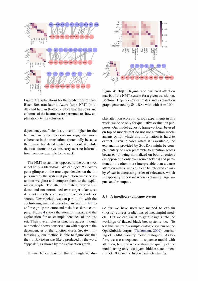
Figure 3: Explanations for the predictions of threeBlack-Box translators: Azure (top), NMT (mid-dle) and human (bottom). Note that the rows andcolumns of the heatmaps are permuted to show ex-planation chunks (clusters).

dependency coefficients are overall higher for thehuman than for the other systems, suggesting morecoherence in the translations (potentially becausethe human translated sentences in context, whilethe two automatic systems carry over no informa-tion from one example to the next).

The NMT system, as opposed to the other two,is not truly a black-box. We can open the box toget a glimpse on the true dependencies on the in-puts used by the system at prediction time (the at-tention weights) and compare them to the expla-nation graph. The attention matrix, however, isdense and not normalized over target tokens, soit is not directly comparable to our dependencyscores. Nevertheless, we can partition it with thecoclustering method described in Section 4.3 toenforce group structure and make it easier to com-pare. Figure 4 shows the attention matrix and theexplanation for an example sentence of the testset. Their overall cluster structure agrees, thoughour method shows conservatism with respect to thedependencies of the function words (to, for). In-terestingly, our method is able to figure out thatthe <unk> token was likely produced by the word“appeals”, as shown by the explanation graph.

It must be emphasized that although we dis-

Dies

würde

<unk> .

gegen

ermöglichen

Urteile

judgementsagainst

madebeto.

appealsfor

allowwouldThis

Dies

würde

<unk> .

gegen

ermöglichen

Urteile

0.00

0.15

0.30

0.45

0.60

Dies

würde

<unk>

ermöglichen

Urteile

gegen .

.aga

instmadeto

judgem

entsbeforappeal

sallowwouldThis

made

würde

for

<unk>

appealsallowwould

ermöglichen

against

.gegen

to judgements

UrteileDies

This .be

Figure 4: Top: Original and clustered attentionmatrix of the NMT system for a given translation.Bottom: Dependency estimates and explanationgraph generated by SOCRAT with with S = 100.

play attention scores in various experiments in thiswork, we do so only for qualitative evaluation pur-poses. Our model-agnostic framework can be usedon top of models that do not use attention mech-anisms or for which this information is hard toextract. Even in cases where it is available, theexplanation provided by SOCRAT might be com-plementary or even preferable to attention scoresbecause: (a) being normalized on both directions(as opposed to only over source tokens) and parti-tioned, it is often more interpretable than a denseattention matrix, and (b) it can be retrieved chunk-by-chunk in decreasing order of relevance, whichis especially important when explaining large in-puts and/or outputs.

5.4 A (mediocre) dialogue system

So far we have used our method to explain(mostly) correct predictions of meaningful mod-els. But we can use it to gain insights into theworkings of flawed black-box systems too. Totest this, we train a simple dialogue system on theOpenSubtitle corpus (Tiedemann, 2009), consist-ing of ∼14M two-step movie dialogues. As be-fore, we use a sequence-to-sequence model withattention, but now we constrain the quality of themodel, using only two layers, hidden state dimen-sion of 1000 and no hyper-parameter tuning.

Input Prediction

What do you mean it doesn’t matter? I don’t knowPerhaps have we met before? I don’t think soCan I get you two a cocktail? No, thanks.

Table 2: “Good” dialogue system predictions.

don't

it

know.

What do

I

doesn't matter?meanyou

I

don't

know.

?

matter

t

'

doesn

it

mean

you

do

What

0.15

0.30

0.45

0.60

0.75

Figure 5: Explanation with S = 50 (left) and at-tention (right) for the first prediction in Table 2.

Although most of the predictions of this modelare short and repetitive (Yes/No/<unk> answers),some of them are seemingly meaningful, andmight—if observed in isolation—lead one to be-lieve the system is much better than it actually is.For example, the predictions in Table 2 suggest acomplex use of the input to generate the output.To better understand this model, we rationalizeits predictions using SOCRAT. The explanationgraph for one such “good” prediction, shown inFigure 5, suggests that there is little influence ofanything except the tokens What and you on theoutput. Thus, our method suggests that this modelis using only partial information of the input andhas probably memorized the connection betweenquestion words and responses. This is confirmedupon inspecting the model’s attention scores forthis prediction (same figure, right pane).

5.5 Bias detection in parallel corpora

Natural language processing methods that derivesemantics from large corpora have been shownto incorporate biases present in the data, suchas archaic stereotypes of male/female occupations(Caliskan et al., 2017) and sexist adjective asso-ciations (Bolukbasi et al., 2016). Thus, there isinterest in methods that can detect and addressthose biases. For our last set of experiments, weuse our approach to diagnose and explain biasedtranslations of MT systems, first on a simplisticbut verifiable synthetic setting, where we inject

is

il

you

penser bon que

think

est

good

peux

However, might

Tu qu

this

<unk>tu

Figure 6: Explanation with S = 50 for the predic-tion of the biased translator.

Tu

peux

penser

qu

il

est

bon

que

tu

<unk>

good

is

this

think

might

you

,

However

Vous

pourriez

penser

que

cela

est

bonne

good

is

this

think

might

you

0.15

0.30

0.45

0.60

Figure 7: Attention scores on similar sentences bythe biased translator.

a pre-specified spurious association into an other-wise normal parallel training corpus, and then onan industrial-quality black-box system.

We simulate a biased corpus as follows. Start-ing from the WMT14 English-French dataset, weidentify French sentences written in the informalregister (e.g. containing the singular second per-son tu) and prepend their English translation withthe word However. We obtain about 6K examplesthis way, after which we add an additional 1M ex-amples that do not contain the word however onthe English side. The purpose of this is to attemptto induce a (false) association between this ad-verb and the informal register in French. We thentrain a sequence-to-sequence model on this pol-luted data, and we use it to translate adversarially-chosen sentences containing the contaminating to-ken. For example, given the input sentence “How-ever, you might think this is good”, the methodpredicts the translation “Tu peux penser qu ’ il estbon que tu <unk>”, which, albeit far from per-fect, seems reasonable. However, using SOCRAT

to explain this prediction (cf. Figure 6) raises a redflag: there is an inexplicable strong dependencybetween the function word however and tokensin the output associated with the informal regis-ter (tu, peux), and a lack of dependency betweenthe second tu and the source-side pronoun you.The model’s attention for this prediction (shownin Figure 7, left) confirms that it has picked up thisspurious association. Indeed, translating the En-glish sentence now without the prepended adverb

very

est

dancer

charmante

This

Cette

charmingis

danseuse très

very

est

doctor

talentueux

This

Ce

talentedis

médecin très sontpersonnes

These are

Ces très

people

bizarres

oddvery

Figure 8: Explanations for biased translations of similar gender-neutral English sentences into Frenchgenerated with Azure’s MT service. The first two require gender declination in the target (French)language, while the third one, in plural, does not. The dependencies in the first two shed light on thecause of the biased selection of gender in the output sentence.

results in a switch to the formal register, as shownin the second plot in Figure 7.

Although somewhat contrived, this syntheticsetting works as a litmus test to show that ourmethod is able to detect known artificial biasesfrom a model’s predictions. We now move to areal setting, where we investigate biases in thepredictions of an industrial-quality translation sys-tem. We use Azure’s MT service to translate intoFrench various simple sentences that lack genderspecification in English, but which require gender-declined words in the output. We choose sentencescontaining occupations and adjectives previouslyshown to exhibit gender biases in linguistic cor-pora (Bolukbasi et al., 2016). After observing thechoice of gender in the translation, we use SO-CRAT to explain the output.

In line with previous results, we observe thatthis translation model exhibits a concerning pref-erence for the masculine grammatical gender insentences containing occupations such as doctor,professor or adjectives such as smart, talented,while choosing the feminine gender for charm-ing, compassionate subjects who are dancers ornurses. The explanation graphs for two suchexamples, shown in Figure 8 (left and center),suggest strong associations between the gender-neutral but stereotype-prone source tokens (nurse,doctor, charming) and the gender-carrying targettokens (i.e. the feminine-declined cette, danseuse,charmante in the first sentence and the mascu-line ce, médecin, talenteux in the second). Whileit is not unusual to observe interactions betweenmultiple source and target tokens, the strengthof dependence in some of these pairs (charm-ing→danseuse, doctor→ce) is unexplained froma grammatical point of view. For comparison, thethird example—a sentence in the plural form that

does not involve choice of grammatical gender inFrench—shows comparatively much weaker asso-ciations across words in different parts of the sen-tence.

6 Discussion

Our model-agnostic framework for prediction in-terpretability with structured data can produce rea-sonable, coherent, and often insightful explana-tions. The results on the machine translation taskdemonstrate how such a method yields a partialview into the inner workings of a black-box sys-tem. Lastly, the results of the last two exper-iments also suggest potential for improving ex-isting systems, by questioning seemingly correctpredictions and explaining those that are not.

The method admits several possible modifi-cations. Although we focused on sequence-to-sequence tasks, SOCRAT generalizes to other set-tings where inputs and outputs can be expressed assets of features. An interesting application wouldbe to infer dependencies between textual and im-age features in image-to-text prediction (e.g. im-age captioning). Also, we used a VAE-based sam-pling for object perturbations but other approachesare possible depending on the nature of the domainor data.

Acknowledgments

We thank the anonymous reviewers for their help-ful suggestions regarding presentation and addi-tional experiments, and Dr. Chantal Melis forvaluable feedback. DAM gratefully acknowledgessupport from a CONACYT fellowship and theMIT-QCRI collaboration.

References

Sebastian Bach, Alexander Binder, Grégoire Mon-tavon, Frederick Klauschen, Klaus-Robert Müller,and Wojciech Samek. 2015. On Pixel-Wise Ex-planations for Non-Linear Classifier Decisions byLayer-Wise Relevance Propagation. PLoS One,10(7):1–46.

Dzmitry Bahdanau, Kyunghyun Cho, and Yoshua Ben-gio. 2014. Neural Machine Translation By JointlyLearning To Align and Translate. Iclr 2015, pages1–15.

Tolga Bolukbasi, Kai-Wei Chang, James Zou,Venkatesh Saligrama, and Adam Kalai. 2016. Manis to Computer Programmer as Woman is to Home-maker? Debiasing Word Embeddings. NIPS,(Nips):4349—-4357.

Samuel R. Bowman, Luke Vilnis, Oriol Vinyals, An-drew M. Dai, Rafal Jozefowicz, and Samy Ben-gio. 2016. Generating Sentences from a ContinuousSpace. Iclr, pages 1–13.

Aylin Caliskan, Joanna J Bryson, and ArvindNarayanan. 2017. Semantics derived automaticallyfrom language corpora contain human-like biases.Science (80-. )., 356(6334):183–186.

Rich Caruana, Yin Lou, Johannes Gehrke, Paul Koch,Marc Sturm, and Noemie Elhadad. 2015. Intelligi-ble Models for HealthCare : Predicting PneumoniaRisk and Hospital 30-day Readmission. Proc. 21thACM SIGKDD Int. Conf. Knowl. Discov. Data Min.- KDD ’15, pages 1721–1730.

William Chan, Navdeep Jaitly, Quoc V. Le, and OriolVinyals. 2015. Listen, attend and spell. arXivPrepr., pages 1–16.

Inderjit s. Dhillon. 2001. Co-clustering documentsand words using Bipartite spectral graph partition-ing. Proc 7th ACM SIGKDD Conf, pages 269–274.

Finale Doshi-Velez and Been Kim. 2017. A Roadmapfor a Rigorous Science of Interpretability. ArXiv e-prints, (Ml):1–12.

Neng Fan, Qipeng P. Zheng, and Panos M. Pardalos.2012. Robust optimization of graph partitioning in-volving interval uncertainty. In Theor. Comput. Sci.,volume 447, pages 53–61.

M. R. Garey, D. S. Johnson, and L. Stockmeyer.1976. Some simplified NP-complete graph prob-lems. Theor. Comput. Sci., 1(3):237–267.

Diederik P Kingma and Max Welling. 2014. Auto-Encoding Variational Bayes. Iclr, (Ml):1–14.

G. Klein, Y. Kim, Y. Deng, J. Senellert, and A. M.Rush. 2017. OpenNMT: Open-Source Toolkit forNeural Machine Translation. ArXiv e-prints.

Yuval Kluger, Ronen Basri, Joseph T. Chang, and MarkGerstein. 2003. Spectral biclustering of microarraydata: Coclustering genes and conditions.

Tao Lei, Regina Barzilay, and Tommi Jaakkola. 2016.Rationalizing Neural Predictions. In EMNLP 2016,Proc. 2016 Conf. Empir. Methods Nat. Lang. Pro-cess., pages 107–117.

Zachary C Lipton. 2016. The Mythos of Model In-terpretability. ICML Work. Hum. Interpret. Mach.Learn., (Whi).

Kevin P. Murphy. 2012. Machine Learning: A Proba-bilistic Perspective.

D J Rezende, S Mohamed, and D Wierstra. 2014.Stochastic backpropagation and approximate infer-ence in deep generative models. Proc. 31st . . . ,32:1278–1286.

Danilo Jimenez Rezende and Shakir Mohamed. 2015.Variational Inference with Normalizing Flows.Proc. 32nd Int. Conf. Mach. Learn., 37:1530–1538.

Marco Tulio Ribeiro, Sameer Singh, and CarlosGuestrin. 2016. "Why Should I Trust You?": Ex-plaining the Predictions of Any Classifier. In Proc.22Nd ACM SIGKDD Int. Conf. Knowl. Discov. DataMin., KDD ’16, pages 1135–1144, New York, NY,USA. ACM.

Alexander M Rush, Sumit Chopra, and Jason Weston.2015. A Neural Attention Model for AbstractiveSentence Summarization. Proc. Conf. Empir. Meth-ods Nat. Lang. Process., (September):379–389.

Ramprasaath R. Selvaraju, Abhishek Das, Ramakr-ishna Vedantam, Michael Cogswell, Devi Parikh,and Dhruv Batra. 2016. Grad-CAM: Why did yousay that? Visual Explanations from Deep Networksvia Gradient-based Localization. (Nips):1–5.

Casper Kaae Sønderby, Tapani Raiko, Lars Maaløe,Søren Kaae Sønderby, and Ole Winther. 2016. Lad-der Variational Autoencoders. NIPS, (Nips).

Jörg Tiedemann. 2009. News from OPUS - A Collec-tion of Multilingual Parallel Corpora with Tools andInterfaces. In N. Nicolov, G. Bontcheva, G. An-gelova, and R. Mitkov, editors, Recent Adv. Nat.Lang. Process., pages 237—-248. John Benjamins,Amsterdam/Philadelphia.

Jörg Tiedemann and Robert Östling. 2016. EfficientWord Alignment with Markov Chain Monte Carlo.Prague Bull. Math. Linguist., (106):125–146.

A Formulation of graph partitioningwith uncertainty

The bipartite version of the graph partitioningproblem with edge uncertainty considered by Fanet al. (2012) has the following form. Assume wewant to partition U and V into K subsets each,say Ui and Vj, with each Ui having cardinal-ity in [cumin, c

umax] and each Vj in [cvmin, c

vmax]. Let

xuik be the binary indicator of ui ∈ Uk, and anal-ogously for xvjk and vj . In addition, we let yij bea binary variable which takes value 1 when ui, vjare in different corresponding subsets (i.e. ui ∈Uk, vj ∈ Vk′ and k 6= k′). We can express theconstraints of the problem as:

Y =

K∑k=1

xvik = 1 ∀i

K∑k=1

xujk = 1 ∀j

cumin ≤N∑i=1

xvik ≤ cumax ∀i

cvmin ≤N∑i=1

xujk ≤ cvmax ∀j

− yij − xvik + xujk ≤ 0 ∀i, j, k− yij + xvik − xujk ≤ 0 ∀i, j, kxvik, x

ujk, yij ∈ 0, 1, ∀i, j, k

(4)

(5)

(6)

(7)

(8)

(9)

(10)

Constraints (4) and (5) enforce the fact that eachsi and tj can belong to only one subset, (6) and(7) limit the size of the Uk and Bk to the speci-fied ranges. On the other hand, (8) and (9) encodethe definition of yij : if yij = 0 then xuik = xvjkfor every k. A deterministic version of the bipar-tite graph partitioning problem which ignores edgeuncertainty can be formulated as:

min(xu

ik,xvik,yij)∈Y

N∑i=1

M∑j=1

wijyij (11)

The robust version of this problem proposed byFan et al. (2012) incorporates edge uncertainty byadding the following term to the objective:

maxS:S⊆V,|S|≤Γ(it,jt)∈J\S

∑(i,j)∈S

aijyij + (Γ− bΓc)wit,jtyit,jt

(12)

where Γ is a parameter in [0, |V |] which adjuststhe robustness of the partition against the con-servatism of the solution. This term essentiallycomputes the maximal variance of a single cut(S, V \ S) of size |Γ|. Thus, larger values of thisparameter put more on the edge variance, at thecost of a more complex optimization problem. Asshown by Fan et al. (2012) the objective can bebrought back to a linear form by dualizing the term(12), resulting in the following formulation

minM∑i=1

M∑j=1

wijyij + Γp0 +∑

(i,j)∈J

pij

s.t. p0 + pij − aijyij ≥ 0, (i, j) ∈ Jpij ≥ 0, (i, j) ∈ Jp0 ≥ 0

(xuik, yvjk, yij) ∈ Y,

(13)

This is a mixed integer programming (MIP)problem, which can be solved with specializedpackages, such as GUROBI.

B Details on optimization and training

Solving the mixed integer programming problem(13) to optimality can be prohibitive for largegraphs. Since we are not interested in the ex-act value of the partition cost, we can settle foran approximate solution by relaxing the optimal-ity gap tolerance. We observed that relaxing theabsolute gap tolerance from the Gurobi default of10−12 to 10−4 resulted in little minimal change inthe solutions and a decrease in solve time of or-ders of magnitude. We added a run-time limit of2 minutes for the optimization, though in all ourexperiments when never observed this limit beingreached.

C Details on the variational autoencoder

For all experiments in Sections 5.3 through 5.5 weuse the same variational autoencoder: a networkwith three layer-GRU encoder and decoder and astacked three layer variational autoencoder con-necting the last hidden state of the encoder and thefirst hidden state of the decoder. We use a dimen-sion 500 for the hidden states of the GRUs and

Sam

plin

gte

mpe

ratu

reα

y

Input: Students said they looked forward to his class . The part you play in making the news is very important .

Pert

urba

tions

Students said they looked forward to his class The part with play in making the news is important .Students said they looked forward to his history . The question you play in making the funding is a important .Students said they looked around to his class . The part was created in making the news is very important .Some students said they really went to his class . This part you play a place on it is very important .Students know they looked forward to his meal . The one you play in making the news is very important .Students said they can go to that class . These part also making newcomers taken at news is very important .You felt they looked forward to that class . The terms you play in making the news is very important .Producers said they looked forward to his cities . This part made play in making the band , is obvious .Note said they looked forward to his class . The key you play in making the news is very important .Students said they tried thanks to the class ; The part respect plans in making the pertinent survey is available .Why they said they looked out to his period . In part were play in making the judgment , also important .Students said attended navigate to work as deep . The issue met internationally in making the news is very important .What having they : visit to his language ? In 50 interviews established in place the news is also important .Transition said they looked around the sense ." The part to play in making and safe decision-making is necessary .What said they can miss them as too . The order you play an making to not still unique .

Table 3: Samples generated by the English VAE perturbation model around two example input sentencesfor increasing scaling parameter α.

400 for the latent states z. We train it on a 10Msentence subset of the English side of the WMT14translation task, with KLD and variance anneal-ing, as described in the main text. We train for onefull epoch with no KLD penalty and no noise term(i.e. decoding directly from the mean vectormu),and start variance annealing on the second epochand KLD annealing on the 8th epoch. We train for50 epochs, freezing the KLD annealing when thevalidation set perplexity deteriorates by more thana pre-specified threshold.

Algorithm 2 Variational autoencoder perturbationmodel for sequence-to-sequence prediction

1: procedure PERTURB(x)2: (µ,σ) = ENCODE(x)3: for i = 1 to N do4: zi ∼ N (µ, diag(ασ))5: xi ← DECODE(zi)6: end for7: return (xi)Ni=1

8: end procedure

Once trained, the variational autoencoder isused as a subroutine of SOCRAT to generate per-turbations as described in Algorithm 2. Given aninput sentence x, we use the encoder to obtain ap-proximate posterior parameters (µ,σ), and thenrepeatedly sample latent representations from thea gaussian distribution with these parameters. Thescaling parameter α constrains the locality of thespace from which examples are drawn, by scalingthe variance of the encoded representation’s ap-proximate posterior distribution. Larger values ofα encourage samples to deviate further away fromthe mean encoding of the input µ, and thus morelikely to result in diverse samples, at the cost ofpotentially less semantic coherence with the origi-nal input x. In Table 3 we show example sentences

generated by this perturbation model on two inputsentences from the WMT14 dataset with increas-ing scaling value α.

D Black-box system specifications

The three systems used in the machine translationtask in Section 5.3 are described below.

Azure’s MT Service Via REST API calls to Mi-crosoft’s Translator Text service provided as partof Azure’s cloud services.

Neural MT System A sequence-to-sequencemodel with attention trained with the Open-NMT library (Klein et al., 2017) on the WMT15English-German translation task dataset. A pre-trained model was obtained from http://www.opennmt.net/Models/. It has two layers,hidden state dimension 500 and was trained for 13epochs.

A human A native German speaker, fluent inEnglish, was given the perturbed English sen-tences and asked to translate them to German inone go. No additional instructions or context wereprovided, except that in cases where the sourcesentence is not directly translatable as is, it shouldbe translated word-to-word to the extent possible.The human’s German and English language mod-els were trained for 28 and 16 years, respectively.