Originally published as: Hamoudi, M., Thébault, E., Lesur, V., Mandea, M. (2007): GeoForschungsZentrum Anomaly Magnetic Map (GAMMA): A candidate model for the World Digital Magnetic Anomaly Map. - Geochemistry Geophysics Geosystems (G3), 8, Q06023 DOI: 10.1029/2007GC001638.

GeoForschungsZentrum Anomaly Magnetic

MAp (GAMMA): A candidate model for the

World Digital Magnetic Anomaly Map

M. Hamoudi, E. Thébault, V. Lesur, and M. Mandea

Abstract

The World Digital Magnetic Anomaly Map (WDMAM) is an ongoing

effort towards the mapping of worldwide available aeromagnetic

data. It is led by a task force of the International Association for

Geomagnetism and Aeronomy (IAGA) and aims at distributing a

global map in printed and digital forms. In this paper, we describe

in details our candidate model which has to be evaluated by the

IAGA task force together with five other candidate maps. After

discussing the quality of the available data, we apply a simple but

effective method to successfully process, reduce and merge

together individual compilations. The near surface data are

corrected using global field models and further refined with a 2D

polynomial corrections. After the upward continuation to 5km

altitude, data are re-sampled to a 3 minutes grid and merged

together. We then calculate a spherical harmonic model up to

degree 199 and analyze the magnetic spectrum of the global map.

This helps us to confirm that wavelengths larger than 400km are

spurious at a global scale in aeromagnetic compilations. Therefore,

we substitute them using a satellite based lithospheric field model

(MF5) to degree 100.

1

1.Introduction

The importance of aeromagnetic and marine magnetic surveys

to understand the geology has been long demonstrated, but a

number of problems remain difficult to solve when considering

regional compilations only. A worldwide magnetic anomaly model

derived from the merging of satellite, airborne, marine and land

magnetic data can provide a comprehensive view of continental-

scale magnetic trends, not available in individual data sets. It also

helps linking widely separated areas of outcrop, unifies disparate

tectonic and geological studies (Reeves and De Witt, 2000, for

instance). Such a global anomaly map will thus be a powerful tool

for further evaluation of the lithospheric structure, geologic

processes and tectonic evolution of continental or oceanic areas

(Vine, 1966). These studies require consistent data sets over

thousands kilometres distances spanning national boundaries.

The World Digital Magnetic Anomaly Map (WDMAM) working

group of IAGA aims at producing a compiled magnetic anomaly

map containing all possible wavelengths useful for geological and

tectonic mapping of the crust. The work presented here is a

candidate model towards the final WDMAM product. The data sets

used in this study were kindly provided by various organizations to

the WDMAM committee (see Table 1). These magnetic compilations

result from the merging of many independent regional magnetic

surveys with various characteristics. Data were recorded at

different epochs and altitudes, often without proper secular

variation or altitude corrections. The existing final compilations

have therefore errors causing significant differences between

adjacent panels. These errors are clearly noticeable along the

2

edges of adjacent surveys where levelling errors dominate. As a

result, long wavelengths in these surveys are partly spurious and

individual compilations do not easily merge.

Large compilations, such as Arctic or the North America grid,

extending at scales of several thousands of kilometres are available

but, so far, the challenge to handle the number of grids and

specifications greatly hampered the attempt to generate a global

view of magnetic anomalies. Moreover, most data are still not

available for various reasons. Nevertheless, thanks to concerted

and persistent efforts during last years, a large number of near-

surface magnetic grids are now available and this allows the

release of the first magnetic anomaly map.

In a first section, we present the specification of each datasets,

the coordinate systems used and, when available, the original main

field reduction and the overall statistics. We also report on

prominent observed inconsistencies. These discussions help us to

define a grid precedence order according to their estimated quality

in section 2. In section 3, we apply a simple and effective method to

merge the individual grids. We correct the large wavelengths by

iteratively adjusting a low-degree main field for different epochs

until minimum mean anomaly intensity is obtained. We adjust the

grid by removing a regional polynomial to the compilation in order

to improve the statistical characteristics of each data distribution.

Following the recommendation of the WDMAM committee, data are

upward continued to 5km above the World Geodetic System 1984

(WGS84) reference ellipsoid and gridded on a 3'x3' grid (about 5km

spacing). We then apply dedicated software in order to knit a

compilation at a global scale. After a brief review of different

available satellite lithospheric field models, we finally apply a

global spherical harmonic filter to remove the non-physical data

points, the remaining large wavelength discontinuities and the last

3

inconsistencies. Wavelengths larger than spherical harmonic

degree 100, corresponding to 400km maximum resolution, are

removed and the currently best CHAMP anomaly field model

available is subsequently added to the grid at 5km altitude.

2.Data sets

We use the data provided to us by the WDMAM committee. We

consider the compilations summarized in Table 1. Some of them are

partially redundant and we discuss below how we deal with the

overlapping areas.

The overall coverage is especially sparse over oceans, but also over

Africa and South America where data exist without being freely

accessible. The available data density greatly varies between the

Northern and the Southern hemisphere and according to regional

characteristics. The data quality over each region is hard to

estimate as very few compilations have complete metadata

information (see Table 1). When available, metadata information

shows compilations to be in different coordinate systems and

projections. All compilations result from the stitching together of

smaller surveys carried out at various altitudes and the individual

panels were, or were not, upward continued to a common altitude.

For some compilations, these information are provided but since in

general the mean altitude, or the mean terrain clearance with

respect to the mean sea level, is not systematically known, we have

no other choice but to upward continue the data in the latest stage

of the final compilation.

Panels inside each individual compilation were derived for different

epochs and reduced with either local polynomials or IGRF/DGRF

models. In most cases, it is difficult to find out which model was

used to reduce the data. The final patch-worked grids are thus

4

prone to mismatch in anomaly shapes and strengths that may easily

be confused with magnetic anomalies. The lack of absolute

reference makes it difficult to restore the large wavelengths. Data

sampling is also not homogeneous. It varies from about 50km and

30km for respectively India and both Africa and South America

grids, to 1km spacing for North America or Australia, for instance.

Determining the grid resolution for each compilation would require

a full spectral analysis that was not performed here. Checking the

consistency between two overlapping grids is therefore challenging

in some areas where the actual resolution is not known. Moreover,

the resolution is usually not homogeneous within the compilations

themselves and some regions artificially appear devoid of small

magnetic anomalies. In future editions of the WDMAM, this

problem should be identified before any interpretation is carried

out.

Three datasets are used for cosmetic reasons until better grids are

provided: part of Africa and South America in the Southern

hemisphere and the north west of Indian grid constructed from

ground stations.

Several versions exist for some compilations. For instance, version

4 of Australian and adjacent marine areas data were considered. In

general, redundant panels were simply removed from the final

dataset if they did not bring resolution improvement. Hence,

Mexico grid was removed as the data were included in the North

American compilation. Japan grid was part of the East Asia

compilation and was not considered. To the contrary, Fennoscandia

and Austria, included in the Arctic and European compilation, have

a better resolution. After a thorough analysis, project Magnet

dataset was removed in order to minimize the associated spurious

effects over North America and Australia. Some compilations such

5

as China or Mongolia were obtained from digitization of shaded

colour maps and thus discarded. In the latter cases, the quality of

the grid could not be objectively testified but visual inspections and

statistics show discontinuities, noise, unrealistic linear features

spreading over thousands of kilometres and obvious edge effects.

Regarding all these aspects, although some grids have interesting

characteristics, only a few files like the French, Italian and Spanish

grid, for instance, posses the complete information to fully control

the data processing. The French grid is also derived from a one-

year survey carried out at a nearly constant altitude and reduced to

3km altitude above mean sea level. Line levelling, main field and

external field corrections using the nearest observatory were

performed (Le Mouël, 1969). The grid also comes with the total

field intensity and, as it slightly overlaps with the European

compilation, we use the French dataset to level the European

compilation near the French boundary. Similarly, the Italian

compilation is a corrected grid provided with the regional

polynomial used to reduce the total intensity (Chiappini et al.,

2000). It is thus possible to further correct for a global core field

model or a given epoch. Information on the core field reduction is

not provided for the Australian compilation, it nonetheless provides

high quality data that are consistent over large scale with satellite

observations.

Before applying filtering and correction procedures, the data not

provided in a geographic coordinate system are converted to the

global WGS84 reference ellipsoid using transformation formula

(Snyder, 1972) and a dedicated software (Oasis Montaj, GeoSoft©).

3.Grid inconsistencies and discontinuities

6

Some problems discussed above, inherent in each grid, are not

directly noticeable but appear simply by displaying the grids on the

sphere. Discontinuities are a major issue visible on all compilation

edges. It is clearly noticeable at the Northern border between the

American compilation and the Arctic compilation, for instance.

Regarding the specificities and the varieties of survey composing

the American NAMAG compilation, and despite the preliminary

CM4 model reduction (Ravat et al., 2003) we expect a poor

resolution for wavelengths greater than 200km. The most evident

discontinuities are between continental and oceanic compilations.

The marine track-lines data suffer from data reduction, line

levelling and instrumental biases that require a full reprocessing

not performed here. The Canary grid has unrealistic magnitudes

that were adjusted using adjacent compilations.

A quick inspection of basic statistics provides further details about

the reliability of each dataset. The statistics help us to define a

precedence order that is later used for merging grids. For some

compilations, as shown in Table 2, the average anomaly intensity

greatly deviates from zero. If in a first approximation we assume a

dominating crustal field for wavelengths smaller than 3000km (i.e.

spherical harmonic degree 15), the intensity anomaly should

average to zero over large distances. In that respect, the Russian

and the South Asia compilations show peculiar statistics with large

anomaly intensity means. This reveals either a poor core field

reduction or spurious long wavelengths. The European compilation

has also a comparatively large mean (~16nT), which leads to large

discontinuities with all surrounding compilations. Nevertheless, the

metadata information indicate that the European compilation was

purposefully reduced with the DGRF1980 and the core field

contributions for spherical harmonic degrees 11-15 explain mostly

this relatively high mean.

7

The standard deviation is usually between 100nT and 200nT over

continents, but the marine data shows a standard deviation

reaching 930nT. This suggests the persistence of noise, bad tracks

or outliers. For this reason, the correlation between marine and

satellite data is particularly poor. One of the reasons is that marine

data are not corrected for external or daily magnetic variations. In

addition, the crossover tracks, recorded at different times over long

periods, are naturally contaminated by the magnetic secular

changes and external fields and large mismatches are observed.

The calculation of the arithmetic sum is informative and shows

how well the residuals distribute around the mean. For a pure

anomaly field, we expect a Gaussian-like distribution with zero

mean. A non symmetric anomaly distribution around the mean

possibly indicates some positive or negative outliers tailing on the

distribution. The marine compilation has the larger arithmetic sum

closely followed by the Russian, the Australian, and the South Asia

compilations. Note that the comparatively high mean for the

European compilation does not imply a particularly high arithmetic

mean, showing evidence that the European grid does not contain

prominent outliers.

4.Partial correction and adjustments

This section introduces the pre-processing designed to improve the

compatibility in the overlapping areas. We did not systematically

analyse the grid consistencies at regional scales except for few

oceanic compilations. Most compilations were obtained by

combining, locating and processing individual survey to generate a

wider compilation. We assumed rather reliable and uniform grid

qualities, unless otherwise stated as for the European grid.

8

4.a.Visual inspection

A rough technique to smooth the inconsistencies is to bin data on a

coarser grid. Here, we keep the original grid as far as possible in

our processing and we try to identify the evident wrong isolated

points or track lines.

For the oceanic compilation, we identified bad tracks spreading

over thousands of kilometres in the Pacific Ocean and we record a

maximum anomaly field up to 45931.7nT. We manually removed

these tracks. We also removed track lines crossing the African

continents showing possible instrumental deficiencies and/or

location problems in the oceanic data. Off shore Senegal, a few

cross-shaped anomalies were removed.

In the Getech South American and the African compilations the

original data have been decimated. The resulting grids have a poor

quality and a low resolution. The Bangui anomaly, for instance, has

a rather unusual shape and it is sometimes difficult to delineate

clearly other well-known anomalies.

The Indian grid based on repeat stations was considerably reduced

and we kept only data following the magnetic map boundaries

published in Qureshy (1982) on the eastern coast.

The European grid as been shifted by few kilometres such that its

anomaly field coincide with known total intensity anomalies over

Germany. This grid has been used only when no other data set was

available over an area.

At last, most of the grids were prone to edge effects possibly

caused by either remaining large wavelengths or a Fourier filtering

over large distances that was performed at the latest stage of their

compilation process. We could not properly identify and correct for

these effects but some anomalies have unusual shapes and are

shifted. Europe and Russia were bounded with dataset having

9

complete metadata information. We were thus able to better

constraint the merging between adjacent grids in these regions.

4.b.Global field correction

Compilations were formerly reduced with different IGRF/DGRF

core field models sometimes followed by 2D polynomial fitting or a

Cartesian Fourier filtering. For a few grids over the European

continent, we have the correct regional polynomial parameters (or

the DGRF model) and sometimes even the total intensity. It was

thus easy to add the exact core field model and to remove the CM4

(Comprehensive model, Sabaka et al., 2004) for the same epoch.

For the other compilations, we tried to restore the closest core field

model by iteratively looking for the lowest residuals at different

epochs after adding a DGRF model (spherical degree 10) and

subtracting the CM4 model to degree 15. The complete period

between 1960 and 2002 was spanned. The Russian compilation

seems to be outside the CM4 time span and the procedure was not

applied. Figure 1 shows a few examples and results at this step.

The residuals have no particular shape but a minimum can be

found (although sometimes not exactly unique). Since we have no

information about the removed model, this ad hoc procedure may

be arguable. Nevertheless, this step improves the data statistics

presented in Table 3 by lowering the mean intensity anomaly

towards zero. When considering the total field intensity data, the

minimum is obvious. For example, the curve for France shows that

the variation of the residual over the 40 years interval is of the

magnitude order of the secular variation. The same result is

obtained for Italy or Spain. This procedure is thus a way to better

correct for the secular variation between the different

compilations. Since original data may contain various artefacts

caused by the different model biases, it is also a mean to reduce

10

the data with the same core field model. In general, the continuity

in overlapping areas between adjacent compilations was improved.

4.c.Regional polynomial correction

In order to further improve the statistics, a regional second order

polynomial is removed from all grids in the WGS84 geographic

reference so that we avoid Cartesian distortion due to the Earth’s

curvature. This was not possible over geographic poles and Arctic

and Antarctic compilations were processed using Cartesian

reference frame instead. The polynomial fitting was not applied to

the Australian compilation where we assumed that the long

wavelengths were valid. Removing a polynomial carries the risk of

destroying all possible correlation between ground and satellite

data as is illustrated below. The spectrum is modified as the

polynomial correction is a function of the grid size but wavelengths

larger than spherical harmonic degree 100 are ultimately filtered

out (see subsection 4.f). After this correction, the grids have

arguably the correct properties characterising anomaly fields; the

average anomaly intensity and the arithmetic sum are almost zero

(Table 3) and the residual histograms resemble a Gaussian

distribution (see Figure 2).

4.d.Upward continuation

The original grids are provided at various but generally constant

altitudes within the same dataset (see Table 1). This may be untrue

for some compilations but this problem could not be addressed

here as correct altitudes cannot be recovered. We applied the filter

at the specified mean altitude. Oceanic datasets were also upward

continued in order to avoid a too sharp transition between ocean-

continent boundaries.

11

The grids smaller than 2000km width, like Argentina, Austria,

Fennoscandia, Italy, France, Mexico and Spain were directly

upward continued to 5km altitude above the geoid. Larger

compilations were split into 2000km by 2000km squares, which

were upward continued individually. This dimension corresponds

to the maximum size for which the Earth's curvature can be

neglected (Nakagawa et Yukutake, 1985). This requires a Nyquist

re-sampling of the original grid on a 2.5km regular grid in a

Cartesian reference frame so that a maximum resolution of 5km is

obtained. The spacing is chosen so that we have the best trade-off

between speed and efficiency. This high re-sampling is probably

unnecessary as none of the data sets has a true 5km resolution. The

upward continued data are then calculated back to the original

geographic data locations. The GeoSoft© algorithm includes a de-

trending of the data and works in the Fourier domain. Each panel

slightly overlap with the adjacent ones and we systematically check

the consistency of the result over the overlapping areas. We cannot

report on noticeable distortion, and the overall statistics in Table 3

are nearly preserved. It is worth noting that after the upward

continuation the edge effects between adjacent grids were not

significantly but slightly enhanced.

4.e.Merging the grids

The merging process does not rely on physical assumptions and

whether merging the neighbouring grids or not is a matter of

choice. We first considered the complete overlap between different

grids in order to obtain a final grid averaging the full available

information. It occurred to us that this procedure was generating

spurious long and intermediate wavelengths in the merged dataset.

Moreover, it gave the same weight to dataset of different qualities,

which was unacceptable. As a result, no more than fifty kilometres

overlap were allowed between redundant datasets. We thus

12

obtained a merged grid smooth and closer to the independent

original grids. Large amount of both North America and Arctic

compilation data were removed. In South Africa, data were cut

when overlapping SaNaBoZi data; whereas in South America, they

were cut when overlapping Argentina data.

The preliminary processing from paragraph 4.a to 4.d reduces the

large discontinuities but does not fully remove them. We use the

grid-knitting tool of GeoSoft© in order to smooth out the transition

between adjacent grids. Some spurious wavelengths are created

that will be mostly filtered out at the last stage of the processing.

We were especially careful when choosing the precedence grid

order. We already argued that French, Italian, and European grids

were easier to process as we have the necessary metadata

information to better control the processing. Merging large

compilations with small compilations includes a risk, because the

adjustment is better constraint by the large compilation even if the

small one has apparently a better quality. Before merging the grids,

we generate compilations with comparable grid sizes.

The precedence order is as follows: French, Italian and Spanish

grids are first merged together. We then built a second grid from

the Finland, Fennoscandian, European and Austrian grids. This two

new compilations were merged together and the grid from Russia,

Eurasia, Middle East, Antarctica and North America were

successively added to the compilation. The remaining grids were

not merged as they did not have overlap with the grids listed

above.

At this stage, a 3'x3' grid is generated using GMT (Wessel and

Smith, 1991, version 4.1.4). Each node of our final grid is

associated to an index corresponding to the data set used to

calculate the anomaly field value at that node (last column of Table

1). When a grid node is associated with several data sets, the given

13

index correspond to the weighted average of the data sets indices.

Compilations without index in Table 1 were not used in our

merging. Marine data were interpolated whenever the data density

was estimated high enough, otherwise left as single track data.

4.f.Final Global filtering Any discontinuity caused by large wavelengths introduced during

the merging can be filtered out at a global scale by a spherical

harmonic transformation. Compilation boundaries are still visible,

especially between Arctic, Oceanic and Australian grids. In

addition, the mismatch between European and Russian compilation

remains. We thus perform a spherical harmonic transform and filter

out wavelengths larger than spherical harmonic degree 100 in our

global grid to replace them with a continuous satellite based model.

Two different techniques were envisaged for filtering and

smoothing the final grid. A first option consists in filtering the grid

using Fourier transforms. This procedure is relatively fast but is a

non-potential method. Thus, the coefficients could not be used for

predicting the three components of the magnetic field. Moreover, it

is difficult to remove remaining non-physical magnetic

measurements. In this section, we consider the magnetic anomaly

field as the projection of the crustal field onto a core field model:

The grid is interpolated on the knots of the sampling theorem given

in Driscoll and Healy (1994), the parameters up to spherical

harmonic degree 199 were obtained by least-squares (maximum

resolution of 80km). For higher degrees, the coefficients are

difficult to obtain and the processing is time-consuming, as the

power is very low. This is due to data gaps and heterogeneous

resolution at the global scale. The anomaly field is linearized and

projected on the 1990 core field, whose coefficients are extracted

from the CM4 model to degree 15 (Sabaka et al., 2004). It is thus

believed that the estimated Gauss coefficients represent better the

14

three components of the magnetic field anomaly. Interestingly,

despite our careful pre-processing, the first iteration shows

evidence of remaining outliers and non-physical data points. This is

characterized by the presence of strong spikes creating oscillations

spreading over large distances. This carries the risk of introducing

artificial anomalies at all wavelengths in our final map. Some extra

points are thus removed from Argentina, Argentina coastline, near

Santa Helena Island and around Madagascar. The procedure was

then redone without apparent other artefacts.

Figure 3 shows that over Western Europe, the European and the

French grids had an important incompatibility that was attenuated

during the processing. The compatibility was improved trough the

filtering and major discontinuities were smoothed out.

In Figure 4 we compare the spectrum of our spherical harmonic

model with the most recent lithospheric field models, MF4, MF4x

(Lesur and Maus, 2006) and MF5 (Maus et al., 2007). The near-

surface WDMAM spectrum can be divided into three parts. The

first part of the spectrum, from degrees 1 to 40, is comparatively

steeper, has an excess of power and is more irregular. This

suggests that large wavelengths are indeed partly spurious even if

the correlation analysis (Figure 5) shows a better agreement than

expected (0.5 in average for these degrees). Degrees 41 to 89 are

more stable and their variation is consistent with satellite-based

spectrum. From degree 90, a small offset is noticeable whose origin

remains unclear. We may venture that some recent grids were

compiled using a satellite based model derived to degree 90 as a

prior information. This could have induced this lack of power.

Indeed, MF5 has a lack of power explained by the processing

applied to satellite data in order to obtain a robust model from

noisy measurements. The spherical harmonic correlation analysis

(Langel and Hinze, 1998) between MF5 and our near-surface model

15

(Figure 5) shows an average correlation for all degree of 0.61 but

again, beyond degree 40 it is more stable and reaches 0.75 for

n=91. We notice a comparatively lack of correlation between

degrees 70 and 75 that we do not explain.

5.Substitution of long wavelengths and

generation of the 3’ grid

In many regions, low-orbiting satellites can map the strength and

the extension of the lithospheric field. Choosing a global magnetic

lithospheric field model is not a trivial task and a systematic quality

analysis is required.

We discard lithospheric field models based only on satellite

missions prior to the Danish Ørsted mission (1999). Langel and

Hinze (1998) give a comprehensive overview of earlier satellite

missions, such as MAGSAT or POGO and their outcomes.

The Danish satellite Ørsted, launched in February 1999, was

followed by CHAMP (July 2000) and SAC-C (November 2000).

Several models, based on these missions sharing comparable

scientific instruments, were proposed in the last decade.

The comprehensive approach (CM4), initiated by Sabaka et al.

(2004), uses all available data from POGO, MAGSAT, Ørsted, and

only scalar data from CHAMP, as well as observatory data, in order

to obtain a comprehensive model. Although the model estimates all

known sources from the core to the magnetosphere, near-

equatorial lithospheric field representation is probably

contaminated by equatorial electrojet signature due to inclusion of

dayside data. Following the same spirit, various magnetic field

sources are considered by POMME 3.1 (Maus et al., 2006) using

quiet time and night-side data only, which help reducing

ionopsheric effects and better stabilize the model at the ground

level to degree 60. Other models present a very good agreement

16

with this lithospheric field (e,g, CHAOS, Olsen et al. (2006) or

BGS/G/L/0706, Thomson and Lesur (2007)). These comprehensive

approaches give rather robust models for the first degrees but are

noisy above degree 50.

Another approach, based on preliminary filtering, strictly focuses

on the lithospheric field representation. The philosophy is to

carefully select and clean the data for non-lithospheric sources.

Maus et al. (2006) used this subjective approach with four years of

CHAMP data to produce MF4, which is derived up to degree 90.

MF4 still shows inconsistencies in the Polar Regions and Lesur and

Maus (2006) managed to constrain independently Polar and Mid-

latitude regions. Recently, a model up to degree 100 (400km

resolution), using only low orbital CHAMP measurements until mid-

2006, was released (Maus et al., 2007). It is worth noting that data

filtering induces a loss of power noticeable when compared with

other satellite based magnetic models but also with aeromagnetic

data. Nevertheless, the MF models have degrees that are arguably

suitable for large wavelengths replacement and we use MF5 to

degree 100 (400km resolution). These are good compromise

between resolution at the ground and smoothness of the

lithospheric field at 5km altitude on the WGS84 ellipsoid. MF5 was

thus added to the final grid and our resulting candidate version for

the World Digital Magnetic Anomaly Map can be seen in Figure 6.

Grid nodes with no aeromagnetic or marine data were filled with

MF5 and their index set to 97.

6.Conclusion

The World Digital Magnetic Anomaly Map is a promising

international effort and an ongoing project. Despite the large

disparities between aeromagnetic compilations, we are able to

produce a candidate model giving the essence of the worldwide

17

magnetic anomaly distribution. The most important breakthrough

to this project will come with the release of data in uncovered

areas. At the present stage, near-surface data gaps are filled in

with satellite based model that may lead to mis-interpretation in

the shape and strength of the magnetic field. In the future, this

problem should be addressed at all scales since data resolution is

very heterogeneous even among aeromagnetic grids. Therefore,

systematic interpretations should be carried out with caution and

only a spectral analysis could help identifying the areas of various

intrinsic resolutions. A spectral gap is thus presently unavoidable

for the wavelengths from 200km to 400km.

A major problem was to deal with oceanic data that suffer from

large and numerous inconsistencies. In particular, we had to

discard project Magnet data that represented too many mismatches

with existing datasets. A full crossover analysis of oceanic data will

be required in the future that will lead to a better line levelling and

resolve the core and external field problems.

Effort continues nowadays to improve both ends of the spectrum

and the upcoming Swarm mission configuration will help better

resolving smaller wavelengths than degree 100. Other intrinsic

problems may arise from compilations and the signal analysis

processes; both could introduce artefacts and non-potential

features. In addition to compilation efforts, more elaborated

inverse problem techniques are being developed to merge together

satellite and ground surface data at regional scales. These

techniques, base on Laplace equation, may prove useful to fill the

spectral gap, to merge adjacent compilations and to clean the

compilation from their non-potential contributions. The latter are

probably of importance as the different grid underwent re-

sampling, decimation and successive non-potential transformations.

18

In addition, applying a modelling scheme will be useful to

homogenise the map resolution.

The upcoming WDMAM editions will greatly benefit from a better

spatial coverage, new satellite data and improvements in data

processing and modelling.

Acknowledgments - We are grateful to all organizations that

kindly distributed aeromagnetic data to the WDMAM committee. K.

Hemant, Monika Korte and Yoann Lequesnel are warmly

acknowledged for there efforts in acquire various datasets and for

useful discussions. This work was supported by the Deutsche

Forschungsgemeinshaft (DFG, SPP1097)

References

Chiappini, M., A. Meloni, E. Boschi, O. Faggioni, N. Beverini, C.

Carmisciano, and I. Marson (2000), On shore - off shore

integrated shaded relief magnetic anomaly map at sea level of

Italy and surrounding areas, Annali di Geofisica, 43(5), 983-989.

Driscoll, J.R. and Healy, D.M. (1994), Computing Fourier

transforms and convolutions on the 2-sphere. Adv. Appl. Maths.

15, 202-250.

Langel, R.A, and Hintze W.J (1998), The magnetic field of the

Earth’s lithosphere - The Satellite Perspective, Cambridge

University Press.

Le Mouël, J. L. (1969), Sur la distribution des éléments

magnétiques en France, PhD Thesis, Université de Paris, Paris.

19

Lesur, V., and S. Maus (2006), A global lithospheric magnetic

field model with reduced noise level in the Polar Regions,

Geophys. Res. Lett., 33, L13304, doi:10.1029/2006GL025826.

Maus, S., M. Rother, C. Stolle, W. Mai, S. Choi, H. Lühr, D.

Cooke, and C. Roth (2006), Third generation of the Potsdam

Magnetic Model of the Earth (POMME), Geochem. Geophys.

Geosyst., 7, Q07008, doi:10.1029/2006GC001269.

Maus, S., H. Lühr, M. Rother, K. Hemant, G. Balasis, P. Ritter and

C. Stolle (2007), Fifth generation lithospheric magnetic field

model from CHAMP satellite measurements, http://www.gfz-

potsdam.de/pb2/pb23/index.html.

Nakagawa, I., T. Yukutake, and N. Fukushima (1985), Extraction

of magnetic anomalies of crustal origin from Magsat data over

the area of Japanese Islands, J. Geophys. Res, 90(B3), 2609-2615

Olsen, N., H. Lühr, T. J. Sabaka, M. Mandea, M. Rother, L.

Tøffner-Clausen, and S. Choi (2006), CHAOS - A Model of Earth

´s Magnetic Field derived from CHAMP, Ørsted, and SAC-C

magnetic satellite data, Geophys. J. Int., 166, 67-75,

doi:10.1111/j.1365-246X.2006.02959.x.

Qureshy, M. N. (1982), Geophysical and Landsat lineament

mapping—an approach illustrated from West Central and South

India, Photogrammetria, 37,

161–184.

Ravat, T., Hildenbrand and W. Roest (2003), New way of

forecasting near-surface

20

Magnetic data: The utility of the comprehensive model of the

magnetic field, The leading edge, 22, 784-785.

Reeves, C.V., and De Wit, M. (2000), Making ends meet in

Gondwana: retracing the transforms of the Indian Ocean and

reconnecting continental shear zones, Terra Nova, 12, 272-280,

doi:10.1046/j.1365-3121.2000.00309.x.

Sabaka, T. J., N. Olsen, and M. Purucker (2004), Extending

comprehensive models of the Earth’s magnetic field with Ørsted

and CHAMP data, Geophys. J. Int., 159(2), 521-547,

Snyder, J.P (1987), Map projections – A working manual, US

Geological Survey,

Professional paper 1395.

Thomson, A., and V. Lesur (2006), An improved geomagnetic

data selection algorithm for global geomagnetic field modelling,

Geophys. J. Int., In press.

Vine, F. J. (1966), Spreading of the Ocean Floor: New Evidence,

Science, l54, 3775, 1405-1515.

Wessel, P., and W. H. F. Smith (1991), Free software helps map

and display data, Eos Trans., AGU, 72, 441.

21

Table 1 Data used in this study and available metadata information.

Compilation name height (m) Coordinate system/projection Reduction References IndexAntarctic N/A Geographic N/A ADMAP, http://www.geology.ohio-state.edu/geophys/admap/ 47Arctic compilation 1000 Geographic Filtered 500km Voreof 41Europe 3000 Lambert conic conforme 30/60-20 DGRF1980 Wonik et al., 2001 17France 3000 Lambert II etendu Total field 1964.5 Le Mouel, 1969 12China Geographic N/A N/AMiddle East 1000 Geographic N/A AAIME, http://home.casema.nl/errenwijlens/itc/aaime/ 31Australia 1000 N/A N/A Geoscience Australia, http://www.ga.gov.au/ 61USSR 500 Geographic VSEGEI 1965 N/ARussia N/A N/A N/A VSEGEI, http://www.vsegei.ru/WAY/247038/locale/EN/ 23South East Asia Geographic N/A CCOP, http://www.ccop.or.th 37North America varying NAD27 CM4 varying NAMAG, http://pubs.usgs.gov/sm/map_map/ 43South Africa (SaNaBoZi) 1000 Geographic N/A SADC, http://www.sadc.fi 71Italy 0 Geographic ItGRF 1979 Chiappini, C., Annali di Geofisica, Vol 45, 5, 2000 3Finland 150 WGS84 DGRF-65 GTK, http://www.gtk.fi 7Fennoscandia WGS84 DGRF-65 GTK, http://www.gtk.fi 11Spain 3000 UTM33N IGRF1987 Socias, I., Earth Planet Sci Lett., 105, 55-64, 1991 5Canary Island 3200 UTM 28N IGRF 1993.79 IGN, Publi. Tec., No35, Madrid, 1996 67Eurasia 5000 Geographic N/A GSC, http://gsc.nrcan.gc.ca 29Austria 5000 GK, M31 N/A GSA, http://www.geologie.ac.at 19Marine track-lines varying Geographic CM4 varying NGDC, http://www.ngdc.noaa.gov/mgg/geodas/trackline.html 83Africa and south america 5000 Geographic Varying IGRF GETECH, http://www.getech.com 89India 5000 Geographic N/A Qreschy, M.N., 1982, Photogrammetria, 37, 161-184. 73India 5000 Geographic N/A GSI,http://www.gsi.gov.in 79Project Magnet 4750 geographic Comprehensive models NGDC, http://www.ngdc.noaa.gov/seg/geomag/proj_mag.shtmlArgentina inland 5000 N/A N/A SEGEMAR,http://www.segemar/gov.ar 53Argentina margin 5000 Geographic N/A Ghidella, DNA, http://www.dna.gov.ar 59MF5 5000 geographic POMME 3.1 http://www.gfz-potsdam.de/pb2/pb23/index.html. 97

22

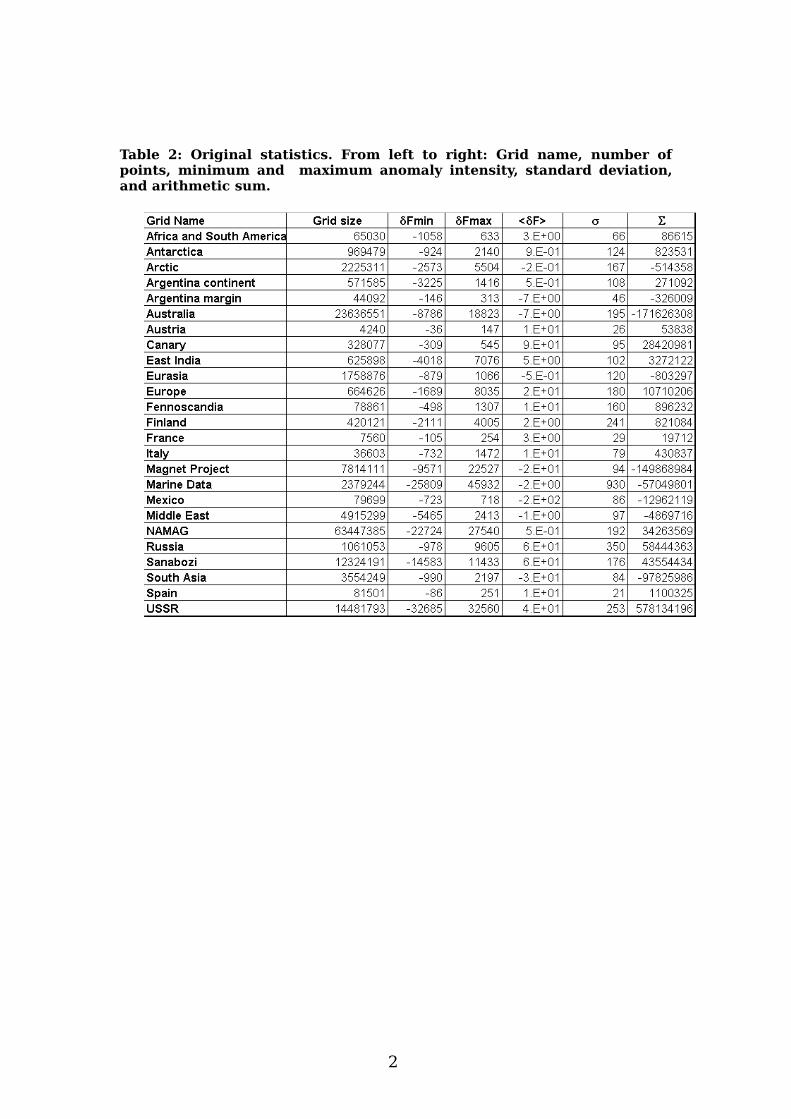
Table 2: Original statistics. From left to right: Grid name, number of points, minimum and maximum anomaly intensity, standard deviation, and arithmetic sum.

23

Table 3: Statistics after pre-processing and outliers correction. Same caption as Table 2.

24

Figure 1: Compilations and individual surveys are iteratively corrected from main field using DGRF and CM4 for each period. The reduction epoch is selected for the minimum anomaly field.

25

Figure 2: Example of an anomaly intensity distribution before and after main field and polynomial corrections for the East Indian grid.

26

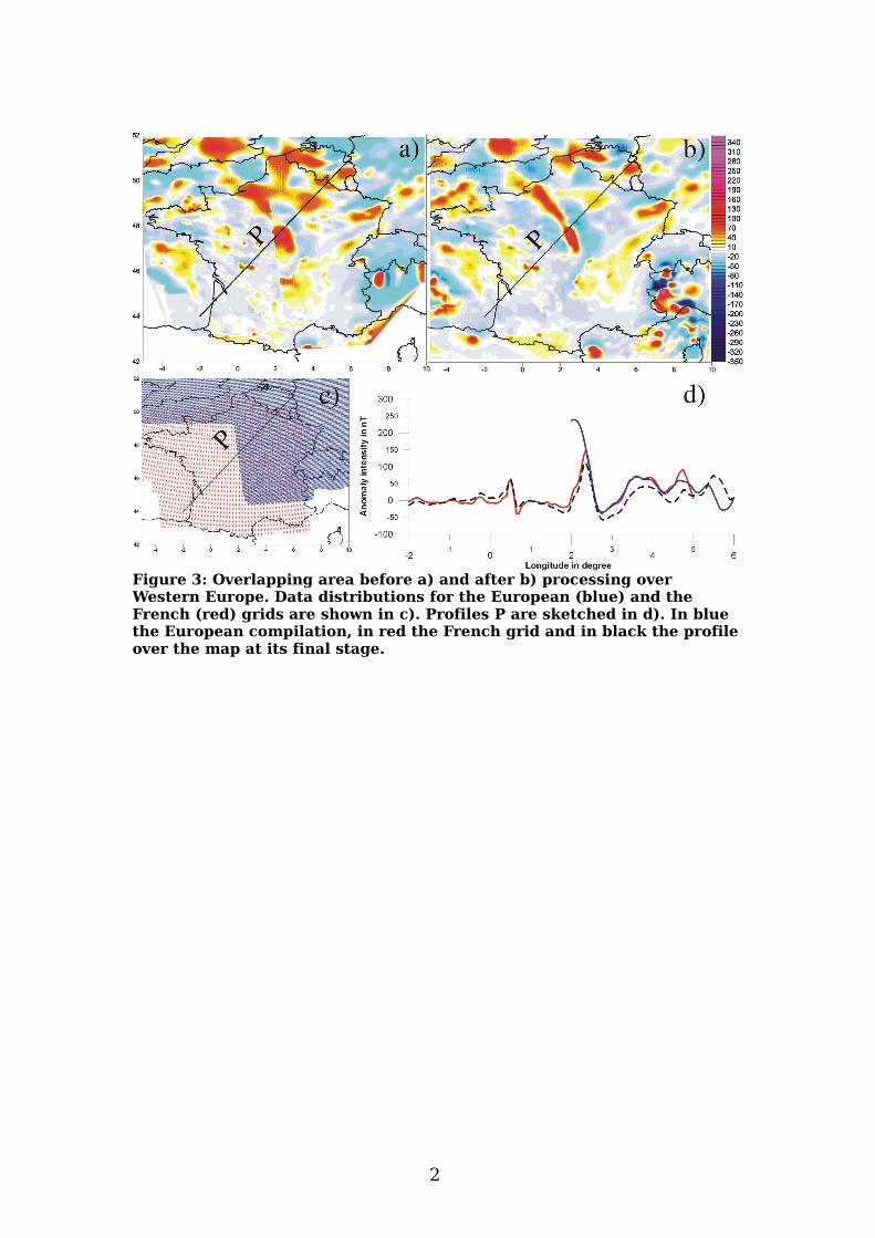
Figure 3: Overlapping area before a) and after b) processing over Western Europe. Data distributions for the European (blue) and the French (red) grids are shown in c). Profiles P are sketched in d). In blue the European compilation, in red the French grid and in black the profile over the map at its final stage.

27

Figure 4: Spectra of the near-surface data and satellite based models. A small increase around degree 90 suggests that some data were reduced with a global field model.

28

Figure 5: Spherical Harmonic Correlation Analysis between ground based and satellite models shows a stable correlation from degree 40.

29

Figure 6: Our candidate WDMAM model in a Mollweide projection (see file attached).

30