a CALIFORNIA IS0 System Operator CALIFORNIA IS0 Callfornla Independent System Operator February...
119
a CALIFORNIA IS0 Callfornla Independent System Operator February 28,2003 Attn: Commission’sDocket Offrce California Public Utilities Commrssron 505 Van Ness Avenue San Francisco,CA 94102 RE: Docket # LOO-1 l-001, Order lnstrtutrng InvestigationInto lmplementatron of Assembly Bill 970 Regardingthe ldentrfrcatron of Electric Transmissionand Drstribubon Constraints,Actronsto Resolve Those Constraints, and Related Matters Affecting the Reliability of Electric Supply Dear Clerk: Enclosedfor filing please find an original and eight copies of the California Independent System Operator Update on a Methodology to Assess the Economic Benefits of Transmission Upgrades in Docket # LOO-1 l-001. Please date stamp one copy and return to Calrfornra IS0 in the self- addressed stamped envelope provided. Thank you. Cc: Attached Service List 151Blue RavineRoad Folsom.California 95630 Telephone 916351.4400
Transcript of a CALIFORNIA IS0 System Operator CALIFORNIA IS0 Callfornla Independent System Operator February...
a CALIFORNIA IS0 Callfornla Independent System Operator
February 28,2003
Attn: Commission’s Docket Offrce California Public Utilities Commrssron 505 Van Ness Avenue San Francisco, CA 94102
RE: Docket # LOO-1 l-001, Order lnstrtutrng Investigation Into lmplementatron of Assembly Bill 970 Regarding the ldentrfrcatron of Electric Transmission and Drstribubon Constraints, Actrons to Resolve Those Constraints, and Related Matters Affecting the Reliability of Electric Supply
Dear Clerk:
Enclosed for filing please find an original and eight copies of the California Independent System Operator Update on a Methodology to Assess the Economic Benefits of Transmission Upgrades in Docket # LOO-1 l-001. Please date stamp one copy and return to Calrfornra IS0 in the self- addressed stamped envelope provided.
Thank you.
Cc: Attached Service List
151 Blue Ravine Road Folsom. California 95630 Telephone 916 351.4400

PROOF OF SERVICE
I hereby certify that on February 28,2003, I served by electronic and U.S. mall the Calforma Independent System Operator Update on a Methodology to Assess the Economic Benefits of Transmwon Upgrades in Docket # I. 00-l l-001.
n DATED at Folsom, California on February 28, 2003.

RICHARD ESTEVES SESCO, INC 77 YACHT CLUB DRIVE, SUITE ,000 LAKE HOPATCONG, NJ 07849-1313
KEITH MC CREA ATTORNEY AT LAW SUTHERLAND, ASBILL 8 BRENNAN 1275 PENNSYLVANIA AVENUE, N w WASHINGTON, DC 20004-2415
KAY DAVOODI NAVY RATE INTERVENTION ,314 HARWOOD STREET, S E WASHINGTON NAVY YARD, DC 20374-5018
SAM DE FRAWI JAMES ROSS REGULATORY 8. COGENERATION SERVICES. A BRUBAKER
NAVY RATE INTERVENTION 1314 HARWOOD STREET, SE INC BRUBAKER & ASSOCIATES. INC
500 CHESTERFIELD CENTER, SUITE 320 1215 FERN RIDGE PARKWAY, SUITE 208 WASHINGTON NAVY YARD, DC 20374-5018 CHESTERFIELD, MO 63017 ST LOUIS, MO 63141
NORMAN A PEDERSEN DANIEL W DOUGLASS ATTORNEY AT LAW ATTORNEY AT LAW HANNA AND MORTON LLP LAW OFFICES OF DANIEL W DOUGLASS 44-l SOUTH FLOWER ST, SUITE ,500 5959 TOPANGA CANYON BLVD , SUITE 244 LOS ANGELES, CA 90071-291s WOODLAND HILLS, CA 91367
CASE ADMINISTRATION LAW DEPARTMENT SOUTHERN CALIFORNIA EDISON COMPANY 2244 WALNUT GROVE AVENUE, ROOM 321 ROSEMEAD, CA 91770
JULIE A MILLER ATTORNEY AT LAW SOUTHERN CALIFORNIA EDISON COMPANY 2244 WALNUT GROVE AVENUE, RM 345 PO BOX 800 ROSEMEAD, CA 9,770
MICHAEL D MACKNESS ATTORNEY AT LAW SOUTHERN CALIFORNIA EDISON CO 2244 WALNUT GROVE AVENUE ROSEMEAD, CA 9,770
JOHN W LESLIE LUCE FORWARD HAMILTON&SCRIPPS, LLP SO0 WEST BROADWAY, SUITE 2600 SAN DIEGO, CA 92101
STACY VAN GOOR STEVEN C NELSON ATTORNEY AT LAW A”ORNEY AT LAW SOUTHERN CALIFORNIA GAS CO 8 SDG&E SEMPRA ENERGY 101 ASH STREET, Ho13 101 ASH STREET SAN DIEGO, CA 92101 SAN DIEGO, CA92101-3017
FREDERICK M ORTLIEB CITY ATTORNEY CARL C LOWER
CITY OF SAN DIEGO THE POLARIS GROUP
,200 THIRD AVENUE, 1 ITH FLOOR 717 LAW STREET
SAN DIEGO, CA 92101-4100 SAN DIEGO, CA 92109-243s
JOSEPH KLOBERDANZ SAN DIEGO GAS & ELECTRIC COMPANY 8330 CENTURY PARK COURT SAN DIEGO. CA 92123
MARY TURLEY REGULATORY CASE ADMINISTRATOR SAN DIEGO GAS & ELECTRIC CO 8315 CENTURY PARK COURT CP22D SAN DIEGO. CA 921231550
BARBARA DUNMORE COUNTY OF RIVERSIDE 4080 LEMON STREET, 12TH FLOOR RIVERSIDE, CA 92501-3651
ROBERT BUSTER SUPERVISOR-DISTRICT 1 COUNTY OF RIVERSIDE 4080 LEMON STREET, 14TH FLOOR RIVERSIDE, CA 92501.365,
HAL ROMANOWITZ OAK CREEK ENERGY 14633 WILLOW SPRINGS ROAD MOJAVE, CA 93501
WILLIAM L NELSON REECH, INC 785 TUCKER ROAD, SUITE G KERN-INYO LIAISON SITE, POSTNET PMB #‘I24 TEHACHAPI. CA 93561
NORMAN J FURUTA ATTORNEY AT LAW DEPARTMENT OF THE NAVY 2001 JUNIPER0 SERRA BLVD , SUITE 600 DALY CITY, CA 94014-3890
KATE POOLE ATTORNEY AT LAW ADAMS BROADWELL JOSEPH a CARDOZO 651 GATEWAY BOULEVARD, SUITE 900 SOUTH SAN FRANCISCO, CA 94080
LONNIE FINKEL ATTORNEY AT LAW ADAMS BROADWELL JOSEPH a CARDOZO 651 GATEWAY BOULEVARD, SUITE 900 SOUTH SAN FRANCISCO, CA 94080
MARC B MIHALY ATTORNEY AT LAW SHUTE MIHALY & WEINBERGER LLP 39s “AYES STREET SAN FRANCISCO, CA 94102
MARCEL HAWIGER ATTORNEY AT LAW MATTHEW FREEDMAN
THE UTILITY REFORM NETWORK TURN
711 VAN NESS AVENUE, SUITE 350 711 VAN NESS AVENUE, NO 350
SAN FRANCISCO, CA 94102 SAN FRANCISCO, CA 94102

OSA ARMI ArTORNF” AT, nw - - .,.. _.... SHUTE MIHALY & WEINBERGER LLP 396 HAYES STREET SAN FRANCISCO. CA 94102
THERESA L MUELLER A”ORNEY AT LAW CITY AND COUNTY OF SAN FRANCISCO CITY HALL ROOM 234 SAN FRANCISCO, CA 94102-4682
CATHERLNE H GILSON ATTORNEY AT LAW FARELLABRAUNBMARTEL, LLP 235 MONTGOMERY STREET RUSS BUILDING, 30TH FLOOR SAN FRANCISCO, CA 94104
WILLIAM” MANHElM ATTORNEY AT LAW PAClFlC GAS AND ELECTRIC COMPANY 77 BEALE STREET, ROOM 3025.B30A SAN FRANCISCO, CA 94105
RICHARD W RAUSHENBUSH ATTORNEY AT LAW LATHAM & WATKINS 505 MONTGOMERY STREET, SUITE 1900 SAN FRANCISCO, CA 94111
DAVID T KRASKA A”ORNEY AT LAW PACIFIC GAS & ELECTRIC COMPANY MAILCODE 630A PO BOX 7442 SAN FRANCISCO, CA 94120.7442
BARRY R FLYNN PRESIDENT FLYNN AND ASSOCIATES 4200 DRIFTWOOD PLACE DISCOVERY BAY, CA 945149267
WILLIAM H BOOT” ATTORNEY AT LAW LAW OFFICE OF WILLIAM H BOOTH ,500 NEWELL AVENUE, 5TH FLOOR WALNUT CREEK, CA 9459s
DIANE FELLMAN ENERGY LAW GROUP, LLP 1999 HARRISON STREET, SUITE 2700 OAKLAND. CA 94612-3572
PATRICK G MCGUIRE CROSSBORDERENERGY 2560 NINTH STREET, SUITE 316 BERKELEY, CA 94710
ROBERT FINKELSTEIN ATTORNEY AT LAW THE UTlLlPl REFORM NETWORK 711 “AN NESS AVE , SUITE 350 SAN FRANCISCO, CA 94102
ITZEL BERRIO ATTORNEY AT LAW THE GREENLINING INSTITUTE 785 MARKET STREET, 3RD FLOOR SAN FRANCISCO. CA 94103-2003
LAURA ROCHE ATTORNEY AT LAW FARELLA, BRAUN & MARTEL, LLP 235 MONTGOMERY STREET RUSS BUILDING, 30TH FLOOR SAN FRANCISCO, CA 94104
DIANE E PRITCHARD ATTORNEY AT LAW MORRISON 8 FOERSTER, LLP 425 MARKET STREET SAN FRANCISCO, CA 941052482
LINDSEY HOW-DOWNING ATTORNFY AT I A W - -. -.... DAVIS WRIGHT TREMAINE LLP ONE EMBARCADERO CENTER, SUITE 600 SAN FRANCISCO, CA 9411 I-3834
SARA STECK MYERS A”ORNEY AT LAW 122 -28TH AVENVE SAN FRANCISCO, CA 94121
MARK J SMITH FPL ENERGY 7445 SOUTH FRONT STREEl LIVERMORE, CA 94550
WILLIAM H CHEN CONSTELLATION NEW ENERGY, INC 2175 N CALIFORNIA BLVD. SUITE 300 WALNUT CREEK, CA 94596
DAVID MARCUS PO BOX 1287 BERKELEY. CA 94702
BARBARA R BARKOVICH BARKOVICH AND YAP, INC 31 EUCALYPTUS LANE SAN RAFAEL, CA 94901
JAMES E SCARFF CALIF PUBLIC UTILITIES COMMISSION 505 VAN NESS AVENUE LEGAL DIVISION ROOM 5121 SAN FRANCISCO, CA 94102.3214
SUSAN E BROWN ATTORNEY AT LAW LATIN0 ISSUES FORUM 785 MARKET STREET, 3RD FLOOR SAN FRANCISCO. CA 941032003
EVELYN K ELSESSER ATTORNEY AT LAW ALCANTAR 8 ELSESSER LLP 120 MONTGOMERY ST, STE 2200 SAN FRANICSCO, CA 94104.4354
BRIAN T CRAGG ATTORNEY AT LAW GOODIN, MACERIDE. SQUERI, RITCHIE 8 DAY 505 SANSOME STREET, NINTH FLOOR SAN FRANCISCO, CA 94111
MICHAEL ALCANTAR ATTORNEY AT LAW ALCANTAR & KAHL LLP 120 MONTGOMERY STREET, SUITE 2200 SAN FRANCISCO. CA 94114
GRANT KOLLING SENIOR ASSlSTANT CITY ATTORNEY CITY OF PALO ALTO PO BOX 10250 PALO ALTO, CA 94303
AL, AMlRALl CALPINE CORPORATION 4160 DUBLIN BLVD DUBLIN. CA 94568
SETH HILTON ATTORNEY AT LAW MORRISON a FOERSTER LLP 101 YGNACIO VALLEY ROAD, SUITE450 WALNUT CREEK, CA 94596-4087
JULIA LEVIN UNION OF CONCERNED SCIENTISTS 2397 SHATTUCK AVENUE, SUITE 203 BERKELEY, CA 94794
JOSEPHM KARP ATTORNEY AT LAW WHITE&CASE LLP THREE EMBARCADERO CENTER, SUITE 2210 SAN FRANCISCO. CA 94941

ROY AND RITA LOMPA 4996 AIRLINE HIGHWAY HOLLISTER, CA 96023
BARRY F MC CARTHY ATTORNEY AT LAW 2106 HAMILTON AVENUE, SUITE 140 SAN JOSE, CA 95125
CHRISTOPHER J MAYER MODESTO IRRIGATION DISTRICT PO BOX 4060 MODESTO, CA 96362.4060
GAYATRI SCHILBERG JEFF NAHIGIAN JBS ENERGY JBS ENERGY, INC 311 D STREET, SUITE A 311 D STREET WEST SACRAMENTO, CA 95605 WEST SACRAMENTO, CA 95605
DOUGLAS K KERNER ELLISON, SCHNEIDER 8 HARRlS 2015 H STREET SACRAMENTO, CA 95614
CALIFORNIA ENERGY COMMISSION JENNIFERTACHERA
,516 NINTH STREET SACRAMENTO, CA 96614
STEVEN KELLY FERNANDO DE LEON
INDEPENDENT ENERGY PRODUCERS ASSN ATTORNEY AT LAW
1215 K STREET SUITE 900 CALIFORNIA ENERGY COMMISSION
SACRAMENTO, CA 95614 1516 NINTH STREET, MS-14 SACRAMENTO, CA 96614-6612
ARLEN ORCHARD ATTORNEY AT LAW SACRAMENTO MUNICIPAL UTILITY DISTRICT PO BOX 15630, MS-B406 SACRAMENTO, CA 96662-1630
MARIA E STEVENS CALIF PUBLIC UTILITIES COMMISSION 320 WEST 4TH STREET SUITE 500 EXECUTIVE DIVISION LOS ANGELES, CA 90013
AARON J JOHNSON CALIF PUBLIC UTILITIES COMMISSION 505 VAN NESS AVENUE EXECUTIVE DIVISION ROOM 5205 SAN FRANCISCO. CA 94102-3214
BRIAN D SCHUMACHER CALIF PUBLIC UTILITIES COMMISSION 505 VAN NESS AVENUE INVESTIGATION, MONITORING & COMPLIANCE BRANCH AREA 4-A SAN FRANCISCO, CA 94102.3214
CHARLES H MAGEE CALIF PUBLIC UTILITIES COMMISSION 505 VAN NESS AVENUE INVESTIGATION, MONITORING & COMPLIANCE BRANCH AREA 4-A SAN FRANCISCO, CA 94102-3214
JESSEAANTE CALIF PUBLIC UTILITIES COMMISSION 506 VAN NESS AVENUE INVESTIGATION, MONITORING 8, COMPLIANCE BRANCH AREA 4-A SAN FRANCISCO, CA 94102.3214
KARENMSHEA CALIF PUBLIC UTILITIES COMMISSION 605 VAN NESS AVENUE INVESTIGATION, MONITORING & COMPLIANCE BRANCH AREA 4-A SAN FRANCISCO, CA 94102-3214
C SUSIE BERLIN ATTORNEY AT LAW MC CARTHY 8 BERLIN, LLP 2005 HAMILTON AVENUE, SUITE 140 SAN JOSE. CA 96126
DENNIS W DE CUIR A”Y AT LAW A LAW CORPORATION 2999 DOUGLAS BLVD. SUITE 325 ROSEVILLE, CA 95661
LYNN M HAUG ATTORNEY AT LAW ELLISON, SCHNEIDER & HARRIS, LLP 2016 H STREET SACRAMENTO, CA 95614
STEVE S RUPP R W BECK, INC 2710 GATEWAY OAKS DR , STE 3005 SACRAMENTO, CA 95633-3502
JAMES C PAINE ATTORNEY AT LAW STOEL RIVES LLP 900 SW FIFTH AVENUE, STE 2600 PORTLAND, OR 97204
DON SCHOENBECK RCS, INC 900 WASHINGTON STREET, SUITE 760 VANCOUVER, WA 96660
BILLIE C BLANCHARD CALIF PUBLIC UTILITIES COMMISSION 505 VAN NESS AVENUE INVESTIGATION, MONITORING & COMPLIANCE BRANCH AREA 4-A SAN FRANCISCO. CA 94102-3214
JAMES LOEWEN CALIF PUBLIC UTILITIES COMMISSION 505 VAN NESS AVENUE DECISION-MAKING SUPPORT BRANCH AREA 4-A SAN FRANCISCO, CA 94102-3214
KELLY C LEE CALIF PUBLIC UTILITIES COMMISSION 505 VAN NESS AVENUE WATER AND NATURAL GAS BRANCH ROOM 4102 SAN FRANCISCO. CA 94102-3214

KENNETH LEWIS LAINIE MOTAMEDI CALIF PUBLIC UTILITIES COMMISSION CALIF PUBLIC UTILITIES COMMISSION 505 VAN NESS AVENUE 505 VAN NESS AVENUE DECISION-MAKING SUPPORT BRANCH DIVISION OF STRATEGIC PLANNING ROOM 4002 ROOM5119 SAN FRANCISCO, CA 94102.3214 SAN FRANCISCO, CA 94102.3214
MEG GOTTSTEIN CALIF PUBLIC UTILITIES COMMISSION 505 VAN NESS AVENUE DIVISION OF ADMINISTRATIVE LAW JUDGE ROOM 5044 SAN FRANCISCO, CA 94102.3214
iS
MICHELLE COOKE CALIF PUBLIC UTILITIES COMMISSION 505 VAN NESS AVENUE DIVISION OF ADMINISTRATIVE LAW JUDGES ROOM 5006 SAN FRANCISCO. CA 94102.3214
MARK ZIERING CALIF PUBLIC UTILITIES COMMISSION 505 VAN NESS AVENUE SPECIAL INVESTIGATIONS STRATEGIC PLANNING BRANCH ROOM 2202 SAN FRANCISCO, CA 94102-3214
OURANIA M VLAHOS CALIF PUBLIC UTILITIES COMMISSION 505 VAN NESS AVENUE LEGAL DIVISION ROOM 5037 SAN FRANCISCO, CA 94102-3214
ROBERT ELLIOl PAMELA NATALONI ROSALINA WHITE CALIF PUBLIC UTILITIES COMMISSION 505 VAN NESS AVENUE PUBLIC ADVISOR OFFICE AREA 2-B SAN FRANCISCO, CA 94102-3214
CALIF PUBLIC UTILITIES COMMISSION 505 VAN NESS AVENUE INVESTIGATION, MONITORING & COMPLIANCE BRANCH AREA 4-A SAN FRANCISCO, CA 94102.3214
CALIF PUBLIC UTILITIES COMMISSION 505 VAN NESS AVENUE LEGAL DIVISION ROOM 4300 SAN FRANCISCO, CA 94102.3214
SCOTT LOGAN CALIF PUBLIC UTILITIES COMMISSION 505 VAN NESS AVENUE ELECTRICITY RESOURCES AND PRlClNG BRANCH ROOM 4209 SAN FRANCISCO. CA 94102.3214
SHYSHENQ P LlOU WENDY M PHELPS CALIF PUBLIC UTILITIES COMMISSION 505 VAN NESS AVENUE INVESTIGATION, MONITORING & COMPLIANCE BRANCH AREA 4-A SAN FRANCISCO, CA 94102.3214
CALIF PUBLIC UTILITIES COMMISSION 505 VAN NESS AVENUE INVESTIGATION, MONITORING & COMPLIANCE 81 ?ANCH AREA 4-A SAN FRANCISCO, CA 94102-3214
XUGUANG LENG CALIF PUBLIC UTILITIES COMMISSION 505 VAN NESS AVENUE INVESTIGATION, MONITORING 8 COMPLIANCE BRANCH AREA 4-A SAN FRANCISCO, CA 94102-3214
SUSAN LEE ASPEN ENVIRONMENTAL GROUP 235 MONTGOMERY STREET, SUITE 600 SAN FRANCISCO, CA 94104
JIM MCCLUSKEY CALIFORNIA ENERGY COMMISSION 15169TH STREET SACRAMENTO, CA 94814
KAREN GRIFFIN MANAGER, ELECTRICITY ANALYSIS CALIFORNIA ENERGY COMMISSION 1516 9TH STREET MS-20 SACRAMENTO, CA 95194
MEG GOTTSTEIN ADMINISTRATIVE LAW JUDGE POBOXZiO 21496 NATIONAL STREET VOLCANO, CA 95689
ALAN LOFASO CALIF PUBLIC UTILITIES COMMISSION 770 L STREET, SUITE ,050 EXECUTIVE DIVISION SACRAMENTO, CA 95814
AUDRA HARTMANN CARLOS A MACHADO CALIF PUBLIC UTILITIES COMMISSION 770 L STREET, SUITE ,050 EXECUTIVE DIVISION SACRAMENTO, CA 95814
GRANT A ROSENBLUM STAFF COUNSEL ELECTRICITY OVERSIGHT BOARD 770 L STREET, SUITE ,250 SACRAMENTO. CA 95814
CALIF PUBLIC UTILITIES COMMlSSlON 770 L STREET, SUITE 1050 EXECUTIVE DIVISION SACRAMENTO, CA 95814
RODERICK A CAMPBELL CALIF PUBLIC UTILITIES COMMISSION 770 L STREET, SUITE 1050 INVESTIGATION, MONITORING & COMPLIANCE BRANCH SACRAMENTO, CA 95814
TOM FLYNN POLICY ADVISOR ELECTRICITY OVERSIGHT BOARD 770 L STREET SUITE 1250 SACRAMENTO. CA 95814
MARK HESTERS CALIFORNIA ENERGY COMMISSION 1519 9TH STREET, MS 46 SACRAMENTO, CA 95814
DON KONDOLEON TRANSMISSION EVALUATION UNlT CALIFORNIA ENERGY COMMISSION 1516 NINTH STREET, MS-46 SACRAMENTO, CA 95814.5512
FERNANDO DE LEON ATTORNEY AT LAW CALIFORNIA ENERGY COMMISSION ,516 9TH STREET, MS-14 SACRAMENTO, CA 95614.5512
JAMES HOFFSIS CALIFORNIA ENERGY COMMISSION ,516 NINTH STREET MS-45 SACRAMENTO, CA 95814-5512
JUDY GRAU CALIFORNIA ENERGY COMMISSION 1516 NINTH STREET MS-46 SACRAMENTO, CA 95814.5512
MELINDA MERRln CALIFORNIA ENERGY COMMISSION 1516 NINTH STREET, MS 45 SACRAMENTO, CA 958145512
PUBLIC UTILITIES COMMISSION OF THE STATE OF CALIFORNIA
Order Instttuting Investtgation mto ) implementation of Assembly Bill 970 regardmg ) the identification of electric transmission and ) dtstribution constraints, actions to resolve those) constraints, and related matters affecting the ) reliability of electrtc supply.
i
1.00-11-001
THE CALIFORNIA INDEPENDENT SYSTEM OPERATOR UPDATE ON A METHODOLOGY TO ASSESS THE ECONOMIC BENEFITS OF TRANSMISSION
UPGRADES
Charles F Robinson, General Counsel Jeanne M. Sole, Regulatory Counsel California Independent System Operator 15 1 Blue Ravine Road Folsom, CA 95630 Telephone: 916-35 l-4400 Facsimile: 916-351-2350
Attorneys for the California Independent System Operator
Dated: February 28,2003
PUBLIC UTILITIES COMMISSION OF THE STATE OF CALIFORNIA
Order Instituting Investigation into 1 implementation of Assembly Bill 970 regarding ) the identification of electric transmlsslon and ) dlstnbutlon constraints, actions to resolve those) constraints, and related matters affecting the ) reliablhty of electric supply.
1.00-11-001
THE CALIFORNIA INDEPENDENT SYSTEM OPERATOR UPDATE ON A METHODOLOGY TO ASSESS THE ECONOMIC BENEFITS OF TRANSMISSION
UPGRADES
In accordance with the Administrative Law Judge’s (“ALJ”) January 29, 2003
Ruling and Notice of Evidentiary Hearings on Tehachapi Transmission Project
(“January 29 Ruling”), the California Independent System Operator (“CA ISO”)
respectfully submits a report on “A Proposed Methodology for Evaluating the
Economic Benefits of Transmission Expansions in a Restructured Wholesale
Electricity Market” (‘Report”). Consistent with the January 29 Ruling, the CA IS0
will be prepared to discuss the report in a workshop to be organized by Pacific Gas
and Electric Company (“PG&E”) currently scheduled for March 14, 2003.
The report describes the methodology developed by the CA IS0 jointly with
London Economics International LLC Y‘LE”) with input and review provided by an
external steering committee -- comprised of representatives from the California
Public Utilities Commission (“CPUC”), the California Electricity Oversight Board
(YEOB”), the California Energy Commission (“CEC”), PG&E, Southern California
Edison Company (“SCE”), and San Diego Gas and Electric Company (“SDG&E”) -
and the CA IS0 Market Surveillance Committee. The report does not contain the
results of illustrative simulations of the estimated benefits of a Path 26 expansion,
because some additional work is required to finalize this information. The CA
IS0 expects to disseminate this information to the service list prior to the March 14
workshop.
February 28,2003 Respectfully Submitted:
Attorney for California Independent System Operator
Charles F. Robinson, General Counsel Jeanne M. Sol& Regulatory Counsel California Independent System Operator 15 1 Blue Ravine Road Folsom, CA 95630 Telephone: 916-351-4400 Facslrmle: 916-351-2350
Attorneys for California Independent System Operator

A Proposed Methodology for Evaluating the Economic Benefits of Transmission Expansions in a Restructured Wholesale Electricity Market
Prepared by
The California IS0 and London Economics International LLC
February 28,2003
TABLE OF CONTENTS EXECUTIVE SUMMARY .............................................................................................. 5
Major Challenges and Solutions.. ........................................................................... 5 Key Modeling Methods .................... ... ... .................. ........................... .......... 7
Network Representation and Modeling Time Horizon.. ......................................... 7 Critical Inputs to the Model.. .................................................................................. 8 Innovative Modeling Components.. ........................................................................ 8 Scenario Selection and Probability Assignments ................................................. 11 Measurmg Net Benefits ........................................................................................ 12 An Illustrative Example using Path 26 ................................................................. 12
INTRODUCTION ........................................................................................................... 14
I. NETWORK REPRESENTATION AND MODELING TIME HORIZON ...... 16
TRANSMISSION NETWORK REPRESENTATION ................................................................ 16 MODELING TIME HORIZON.. .......................................................................................... 17
II. CRITICAL INPUT COMPONENTS ............................................................... 19
MODELING GAS PRICES ................................................................................................. 19 MODELING DEMAND FORECASTS .................................................................................. 21 MODELING NEAR-TERM NEW GENERATION ENTRY AND RETIREMENTS.. ...................... 23 MODELING LONG-TERM ENERGY CONTRACTS .............................................................. 25 MODELING TRANSMISSION LIMITS FOR PATH 15 AND PATH 26.. ................................... 26
III. CRITICAL MODELING COMPONENTS ..................................................... 28
MODELING IMPORTS. ..................................................................................................... 28 Modeling Southwest Imports. .......................................................................... 29
Observed import patterns.. .................................................................................... 29 The basic model.. .................................................................................................. 30
Modeling Northwest Imports __ __ ....................... ,_ ____ .................... .............. 32 Basic assumptions. ................................................................................................ 32
MODELING CALIFORNIA HYDROLOGY ........................................................................... 34 MODELING OPTIMAL GENERATION DISPATCH.. ............................................................. 39 MODELING DEMAND PRICE RESPONSIVENESS ............................................................... 41 MODELING LONG-TERM NEW GENERATION ENTRY ...................................................... 42
En@ Decision ................................................................................................. 42 MODELING MARKET POWER.. ........................................................................................ 45
Game Theoretic Models .................................................................................... 46 Empirical Approach __ ................. ....................... .................... ....... 49
Stepl: Price-cost Markup Regression Analysis.. .................................................. 50 Step 2: Calculate system variables for the prospective study period.. ................ .61 Step 3: Estimatmg the price-cost markups.. .......................................................... 67 Step 4: Calculating new generation investment.. .................................................. 68
IV. SELECTION OF SCENARIOS ........................................................................ 69
SELECTION OF DEMAND AND NATURAL GAS PRICE SCENARIOS.. ................................. 70 Step 1 -Importance Sampling of 13 Joint Demand/Gas Price Scenarios .............. 70
CAISO & LE Transmisszon Valuation Methodology 2
Step 2: Latm Hypercube Samplingfor Additional Demand/Gas Scenarios 71 SELECTION OF GENERATION ENTRY AND RETIREMENT SCENARIOS . . . . . . . . . . . . . . . . . . . . . . . . . . . . . . 12 SELECTJON OF HYDROLOGY SCENARIOS . . . . . . . . . . . . . . . . . . . . . . . . . . . . . . . . . . . . . . . . . . . . . . . . . . . . . . . . . . . . . . . . . . . . . . . . 74
V. ASSIGNING PROBABILITIES TO SCENARIOS . . . . . . . . . . . . . . . . . . . . . . . . . . . . . . . . . . . . . . . . . . . . 76
Stage 1: Determining joint probabilities for demand and gas price scenarios...... 78 Stage 2 - Assigning Jomt Probabilities to Demand/Gas Price and New Generation Entry by LP t.......................................................................................................... 83
VI. MEASURING NET-BENEFITS . . . . . . . . . . . . . . . . . . . . . . . . . . . . . . . . . . . . . . . . . . . . . . . . . . . . . . . . . . . . . . . . . . . . . . . 85
INTRODUCTION . . . . . . . . . . . . . . . .._._.......................................................................................... 85 THE OPTIMAL INVESTMENT RULE . . . . . . . . . . . . . . . . . .._............................................................... 85
Overview 85 PRODUCER AND CONSUMER SURPLUS AS MEASURES OF BENEFIT . . . . . . . . . . . . . . . . . . . . . . . . . . . . . . . . . . 86
Appkation to transmission investment .._ ._,,__,___ __ __ 87 Distributzonal effects 88
MEASURING COSTS . . . . . . . . . . . . . . . . . . . . . . . . . . . . . . . . . . . . . . . . . . . . . . . . . . . . . . . . . . . . . . . . . . . . . . . . . . . . . . . . . . . . . . . . . . . . . . . . . . . . . . . . 92 SOCIAL DISCOUNT RATE ___._.__.__..................................................................................... 92
VII. SUMMARY OF METHODOLOGY . . . . . . . . . . . . . . . . . . . . . . . . . . . . . . . . . . . . . . . . . . . . . . . . . . . . . . . . . . . . . . . . . 94
CAB0 & LE Transmission Valuation Methodology
Figure 1. Figure 2. Figure 3. Fzgure 4. Figure 5 Figure 6 Figure 7. Figure 8. Figure 9.
c-EC’~ Long-term LOad Forecast Error ________________________________________-- 17 Forecasted Gas Prices for Southern and Northern Caltfornia---------------- 20 Forecasted peak Demand Levels (m) ________________________________________-- 22
ForecastedAnnual Consumption Levels (GWh) -------------------------------- 22 Assumed Near-term New Generation En@ ______________________________________ 23 Near-term plant Ret,,.ements ________________________________________--------------- 24 Assignment of CDWR Long-term Contract ______________________________________ 25 Nominal Transmission Limits for Path 15 and Path 26------------------------ 26 ETC Adjusted Limits for Path 15 and Path 26----------------------------------27
Fgm IO. Kelatton of Southwest Imports to CAISO Loads------------------------------------ 29 Ftgure II Esttmated SW Imports versus CAISO Load----------------------------------- 31 Figure 12. Annual NWEnerB Budgets (MWh/Year) _____________________________________ 32 Figure I3 Regression Results of Monthly Maxzmum Hydro Productton -------------- 35 Ftgure 14. Maxtmum Hydro Output versus Monthly Hydro Productton (MP15) -----36 Figure 15. Impact of Assuming Lower Hydro Capaciv ---------------------------------- 36 Ftgure I6 Hydrology assumptions by year (G Wh top table, MW bottom table) * ---- 3 7 Ftgure 17. Comparrson of CEC Annual Hydro Production to Simulation Quantities38 Figure 18. Monthly Energy Budgets from April 1998December 2000 ---------------- 38 Figure 19. Capital Cost of Base Unit (CCGT) ________________________________________----- 43 Figure 20. Capital Cost of a Peaking Unit (SCGT) _______________________________________ 44 Figure 21. RSI Duration Curve for NP15 and SPl5 (Nov99-OctOO) ------------------ 58 Figure 22. prrce-cost Markup Regression Results ________________________________________ 59 Fqqre 23 Comparison of Actual and Predicted Lerner Indexes -------------------------- 60 Figure 24. Process for Modeling New Generation Entty -------------------------------- 68 Ftgure 25. Demand and Gas price Comblnation,y ______...__.__..-_-_____________________- 70 Ftgure 26. Latrn Hypercube Sampling of Demand and Gas Price Scenarios --------- 71 Ftgure 2 7. Demand and Gas Prtce Combmations (Steps I and 2 Combined) -------- 72 Ftgure 28. Fmal Set of Scenarios used m the Illustrattve Assessment of Path 26 ---- 74 F,gure 29 Study Assumptions on Annual CA Hydro Productron -------------------------- 75 Fzgure 30 CA Annual ffydro productron (1984-2002) _- ___________________________________ 76 Figure 31. Demand and Gas Price Scenarios from Step I of Scenario Selection ---- 78 Figure 32 Formulation of Moment Conszstent LP Approach ------------------------------ 80 Figure 33. Demand and Gas Price Estimated Forecast Errors ------------------------- 81 Ftgure 34. Estrmated Joint Probabilities of Demand and Gas Prices------------------ 82 Figure 35. Objective Function for Second Stage LP ________________________________________- 83 Figure 36. Consumer and pro&-er surplus _____ -__------_- ________________________________ 8 7 Figure 3 7. Impact of a transmission link between zones --------------------------------- 88 Figure 38. Impact of monopoly pricing ________________________________________------------- 89 Figure 39. Benefit Objective Functions ________________________________________------------- 90
Figure 40. path 26 Expansion Capital Costs ________________________________________------ 92 Figure 41. Schematic of Methodology ________________________________________--------------- 95
Table of Figures
CAISO & LE Transmission Valuation Methodology 4
Executive Summary Since September 2001, the CAISO has been working ]olntly with London Economics International LLC (LE) to develop a comprehensive methodology for evaluating the economic benefits of transmission investments in a restructured electricity market. Unlike the prior vertically integrated regime, the restructured wholesale electric market involves a variety of parties making decisions that affect the utilization of transmission lines. This paradigm shift requires a new approach to evaluating the economic benefits of transmission expansions. Specifically, a new approach must address the impact a transmission expansion would have on Increasing transmisslon users’ access to generation sources and demand areas, the impact on incentives for new generation investments, and the impact on increasing market competition. It must also address the inherent uncertainty associated with other critical market drivers such as future hydro conditions, natural gas prices, and demand growth as well as capture the dispatch capability of hydroelectric generation and the availability of import suppltes. These last two factors are particularly critical in modeling the California market given its heavy dependence on hydroelectric generation and Imports. Integrating all of these critical modeling requirements into a comprehensive methodological approach has been extremely challenging.
The methodology presented in the document, which represents the culmination of over a year of joint research between the CAISO and LE with input and review provided by an external steering committee’ and CAISO Market Surveillance Committee, integrates all of these critical modeling requirements into a single comprehensive methodology and demonstrates aspects of the methodology using a proposed expansion of Path 26 as an illustrative case study’. We believe the methodology provided here far exceeds anything that has been done to date in the area of transmission planning studies and that this modeling framework can provide a template for the basic components that a transmission study should address. While much of the focus of this paper is on modeling California transmission projects, the basic approach could be easily adopted to study the benefit of upgrades in other areas of the Western Interconnect.
Major Challenges and Solutions
This evaluation method was developed to capture the benefits of transmission expansion in the current restructured environment. It reflects the transformation
1 The external steering committee conslsted of representatives of the Investor owned utlllbes (SDG&E, SCE, and PG&E) and various state agencies (CPUC, CEC, and the Electnclty OversIght Board (EOB))
2 Various components of this methodology are applied usmg a proposed expansion of Path 26 as an lllustratwe case study. However, lllustratlve slmulatlons of the esbmated benefits of the Path 26 expansion are not prowded and will Instead be provided prior to the PG&E workshop scheduled for March 14, 2003 It IS Important to note that the InformatIon provided for Path 26 IS for lllustratlve purposes only. Some ltmtted scenarios of a Path 26 expansion are evaluated to demonstrate how the methodology works More scenario analysis and possibly a more detalled model of the transmlsslon network would be required for a definitive assessment of a Path 26 expansion.
CAISO & LE Transmission Valuation Methodology 5
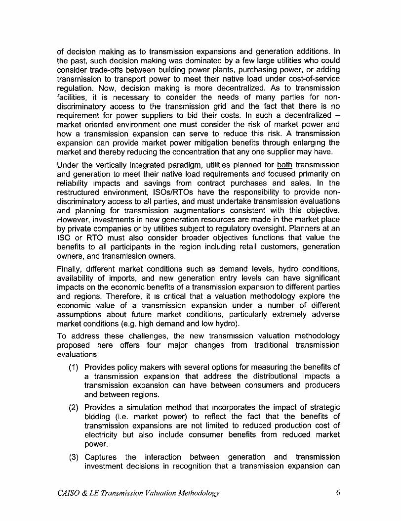
of decision making as to transmission expansions and generation additions. In the past, such decision making was dominated by a few large utilities who could consider trade-offs between burlding power plants, purchasing power, or adding transmission to transport power to meet their native load under cost-of-service regulation. Now, decision making is more decentralized. As to transmission facilities, it is necessary to consider the needs of many parties for non- discriminatory access to the transmission grid and the fact that there is no requirement for power suppliers to bid their costs. In such a decentralized - market oriented environment one must consider the risk of market power and how a transmission expansion can serve to reduce this risk. A transmission expansion can provide market power mitigation benefits through enlargrng the market and thereby reducing the concentration that any one supplier may have.
Under the vertically integrated paradigm, utilities planned for & transmrssion and generation to meet their native load requirements and focused primarily on reliability impacts and savings from contract purchases and sales. In the restructured environment, ISOs/RTOs have the responsibility to provide non- discriminatory access to all parties, and must undertake transmission evaluations and planning for transmission augmentations consistent with this objective. However, investments in new generation resources are made in the market place by private companies or by utilities subject to regulatory oversight. Planners at an IS0 or RTO must also consider broader objectives functions that value the benefits to all participants in the region including retail customers, generation owners, and transmission owners.
Finally, different market conditions such as demand levels, hydro conditions, availability of imports, and new generation entry levels can have significant impacts on the economic benefits of a transmission expansion to different parties and regions. Therefore, it IS critical that a valuation methodology explore the economic value of a transmission expansion under a number of different assumptions about future market conditions, particularly extremely adverse market conditions (e.g. high demand and low hydro).
To address these challenges, the new transmrssion valuation methodology proposed here offers four major changes from traditional transmission evaluations:
(1) Provides policy makers with several options for measuring the benefits of a transmission expansion that address the distributional impacts a transmission expansion can have between consumers and producers and between regions.
(2) Provides a simulation method that incorporates the impact of strategic bidding (i.e. market power) to reflect the fact that the benefits of transmission expansions are not limited to reduced production cost of electricity but also include consumer benefits from reduced market power.
(3) Captures the interaction between generation and transmission investment decisions in recognition that a transmission expansion can
CAB0 & LE Transmission Valuation Methodology 6
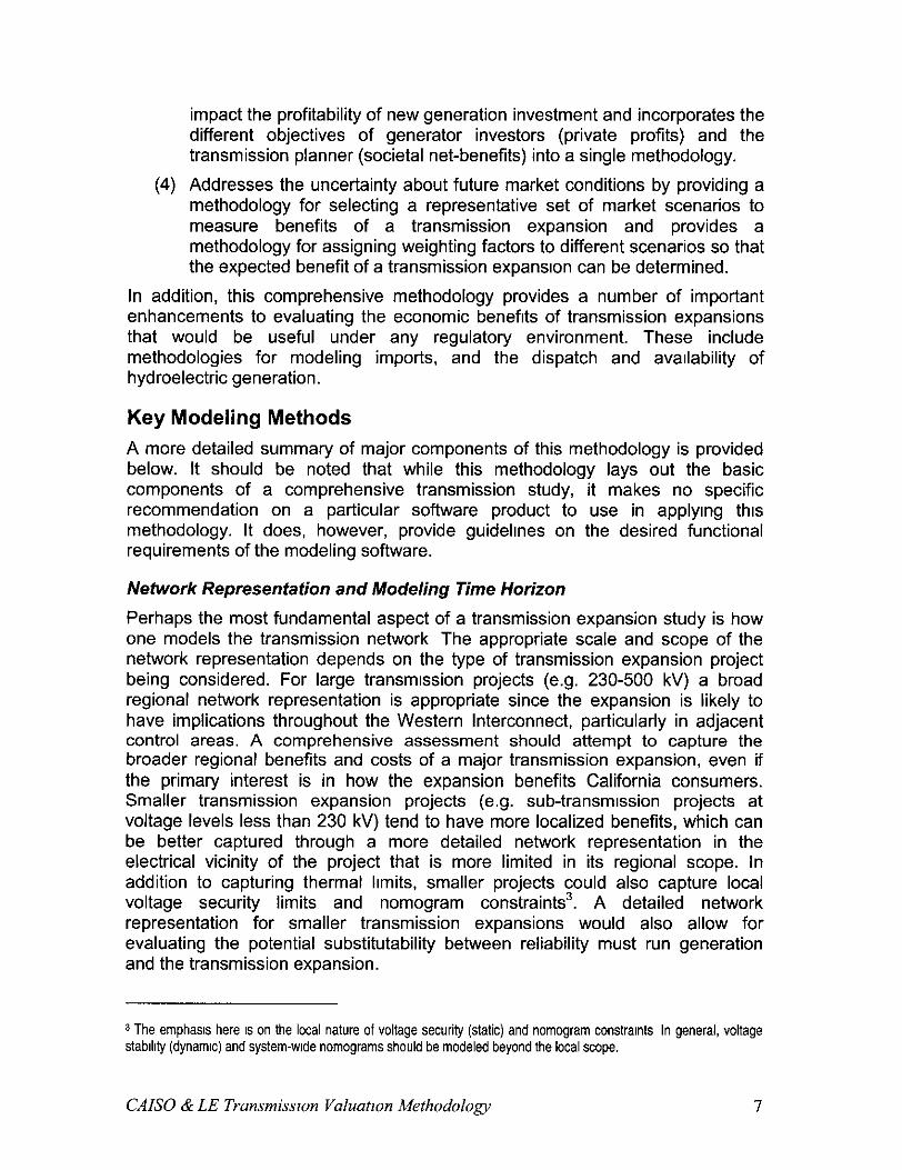
impact the profitability of new generation investment and incorporates the different objectives of generator investors (private profits) and the transmission planner (societal net-benefits) into a single methodology.
(4) Addresses the uncertainty about future market conditions by providing a methodology for selecting a representative set of market scenarios to measure benefits of a transmission expansion and provides a methodology for assigning weighting factors to different scenarios so that the expected benefit of a transmission expansron can be determined.
In addition, this comprehensive methodology provides a number of important enhancements to evaluating the economic benefits of transmission expansions that would be useful under any regulatory environment. These include methodologies for modeling imports, and the dispatch and availability of hydroelectric generation.
Key Modeling Methods A more detailed summary of major components of this methodology is provided below. It should be noted that while this methodology lays out the basic components of a comprehensive transmission study, it makes no specific recommendation on a particular software product to use in applyrng this methodology. It does, however, provide guidelines on the desired functional requirements of the modeling software.
Network Representation and Modeling Time Horizon
Perhaps the most fundamental aspect of a transmission expansion study is how one models the transmission network The appropriate scale and scope of the network representation depends on the type of transmission expansion project being considered. For large transmission projects (e.g. 230-500 kV) a broad regional network representation is appropriate since the expansion is likely to have implications throughout the Western Interconnect, particularly in adjacent control areas. A comprehensive assessment should attempt to capture the broader regional benefits and costs of a major transmission expansion, even if the primary interest is in how the expansion benefits California consumers. Smaller transmission expansion projects (e.g. sub-transmission projects at voltage levels less than 230 kV) tend to have more localized benefits, which can be better captured through a more detailed network representation in the electrical vicinity of the project that is more limited in its regional scope. In addition to capturing thermal limits, smaller projects could also capture local voltage security limits and nomogram constraints3. A detailed network representation for smaller transmission expansions would also allow for evaluating the potential substitutability between reliability must run generation and the transmission expansion.
3 The emphasis here IS on the local nature of voltage security (static) and nomogram constramts In general, voltage stabMy (dynamic) and system-wde nomograms should be modeled beyond the local scope.
CAB0 & LE Transmissron Valuation Methodology 7

Determining an appropriate modeling time horizon is also an important consideration in transmission expansion valuation studies. From a practical standpoint, long-run forecasts covering periods in excess of 8-10 years are subject to substantial forecast error. Because the accuracy of the base-line input assumptions used in the model diminish significantly for long-term projections, it is critical that the benefits of the transmission expansion be evaluated under a number of different input assumptions (i.e. scenarios). Assessing the benefits under a variety of input assumptions can compensate for the inherent uncertainty of these parameters and allow for the estimation of a reasonable range of expected values. In determining an appropriate study period, one needs to also consider when the transmission expansion can be completed. Most transmission projects typically take several years to complete. We belleve a study period In the range of 12-15 years, beginning with the next full calendar year is a reasonable time horizon for a transmrssion expansion study. Benefit estimates beyond this range would be highly speculative due to the uncertainty of future system conditions. Assumrng an average transmission development time of 6 years, a time horizon of 12-15 years would provide 6-9 years of annual benefit estimates. However, a shorter time horizon can be appropriate if a transmission project can be shown to be economically viable within a shorter time frame.
Critical Inputs to the Model
Assumptions about future gas gnces, demand, near-term new generation entry, available transmission capacity , and the degree that buyers are hedged through long-term energy contracts have a significant impact on the estimated economic benefits of a transmission expansion. This document provides some specific recommendations for determining these input data and describes the methodology and data sources used in the illustrative Path 26 expansion analysis. The basic criteria used to select input data is to select the most plausible series of inputs to use as a “base-case” scenario; and to supplement the base-case assumptions with a number of plausible extreme scenarios (e.g. extremely high demand, extremely high gas prices). Capturing extreme scenarios IS tmportant because the benefits of a transmission expansion are often greatest under extreme conditions.
Innovative Modeling Components
The major modeling components of a transmission expansion study include, simulating the availability of imports and exports, modeling the availability and optimal dispatch of hydroelectric and thermal generation, modeling long-term new generation entry, and modeling market power. This document provides methodological approaches to modeling each of these critical components and demonstrates each using a Path 26 expansion as an illustrative case study.
4 Specrf~cally, assumptions about the future utlllzatlon of exlstmg transmwon contracts (ETCs) can have significant implications on the amount of transmwon capaclty that IS assumed “available” to the market.
CAISO & LE Transmission Valuation Methodology 8

Simulating the availability of imports to California must recognize the fundamental characteristics of the two major regions that export to Cakfornia, the Pacific Northwest, and the Desert Southwest. Generation in the Pacific Northwest is predominately hydroelectric and is therefore highly variable from year to year, depending largely on snow-pack and reservoir storage conditions. Also, unlike California, demand for electricity in the Pacific Northwest peaks in the winter months and is generally moderate in the summer months. Because of these characteristics, the Pacific Northwest typically has surplus generation available to export to California during summer and early fall periods but the amount of this supply is extremely variable from year to year. In contrast, the Desert Southwest is predominately thermal based generation and its peak demand tends to coincide with California’s peak demand. As a consequence, during summer months, the availability of imports from the Desert Southwest is often inversely related to the level of demand In California. This document provides methodologies for capturing the unique supply attributes of each of these two regions.
How one models the availability and optimal dispatch of hydroelectric generation within California can have important implrcations on the model results. A methodology for modeling hydroelectric generation must recognize that these resources are typically energy limited (i.e. energy production is limited by the availability of water) and as a consequence, the optimal dispatch must reflect inter-temporal opportunity costs (i.e. the cost of the energy produced today should reflect the foregone market opportunity of selling that energy in some future period). An opportunity cost approach to dispatching hydroelectric supply will optimize the value of hydroelectric production by dispatching it in the highest priced periods. In modeling hydroelectric dispatch one must also recognize that the maxrmum production capabilrties of these resources in any particular hour often depends on the overall hydrology conditions. In very dry years, the maximum hourly production capabilities of some facilities is limited due to a lack of river flow or pond storage. This document provides an opportunity cost approach for modeling hydroelectric dispatch and a methodology for matching the maximum output of hydroelectric resources with overall hydrology conditions.
Modeling the availability and dispatch of thermal resources is relatively straightforward compared to hydroelectric resources. However, a sound methodology for modeling and dispatching thermal generation should include random plant outages and a unit commitment program (i.e. large thermal units with long and expensive start-up costs are only turned on (committed) if market revenues over a 24-hour period are sufficient to cover the unit’s start-up and other operating costs). The frequency and duration of plant outages should be calibrated to be historically consistent the class and vintage of the units (i.e. 40- year old steam units would be expected to experience higher outage rates of longer duration than a new combined cycle unit). It should also be capable of incorporating energy limitations associated with environmental restrictions.
One of the more challenging aspects of developing a methodology for evaluating the economic benefits of transmission expansions concerns the interdependence
CAISO & LE Transmission Valuation Methodology 9
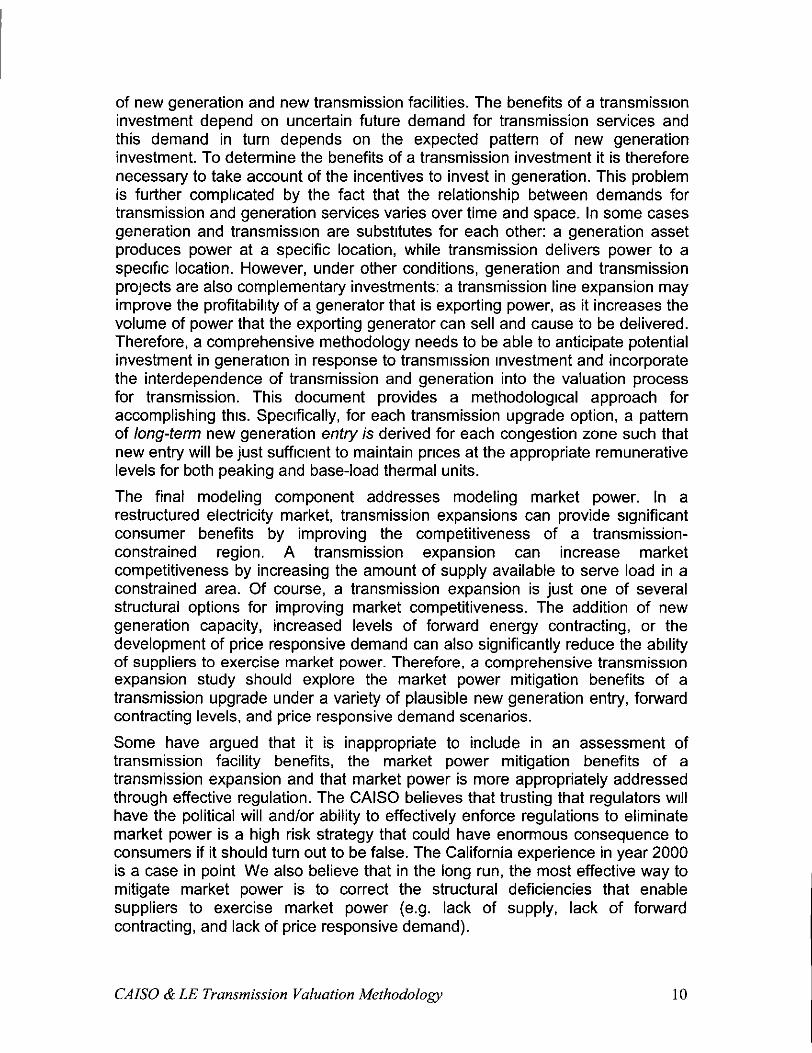
of new generation and new transmission facilities. The benefits of a transmissron investment depend on uncertain future demand for transmission services and this demand in turn depends on the expected pattern of new generation investment. To determine the benefits of a transmission investment it is therefore necessary to take account of the incentives to invest in generation. This problem is further complicated by the fact that the relationship between demands for transmission and generation services varies over time and space. In some cases generation and transmissron are substrtutes for each other: a generation asset produces power at a specific location, while transmission delivers power to a specrfrc location. However, under other conditions, generation and transmission projects are also complementary investments: a transmission line expansion may improve the profitabilrty of a generator that is exporting power, as it increases the volume of power that the exporting generator can sell and cause to be delivered. Therefore, a comprehensive methodology needs to be able to anticipate potential investment in generation in response to transmission investment and incorporate the interdependence of transmission and generation into the valuation process for transmission. This document provides a methodological approach for accomplishing thus. Specifically, for each transmission upgrade option, a pattern of long-term new generation entry is derived for each congestion zone such that new entry will be just sufficient to maintain prices at the appropriate remunerative levels for both peaking and base-load thermal units.
The final modeling component addresses modeling market power. In a restructured electricity market, transmission expansions can provide significant consumer benefits by improving the competitiveness of a transmission- constrained region. A transmission expansion can increase market competitiveness by increasing the amount of supply available to serve load in a constrained area. Of course, a transmission expansion is just one of several structural options for improving market competitiveness. The addition of new generation capacity, increased levels of forward energy contracting, or the development of price responsive demand can also significantly reduce the ability of suppliers to exercise market power. Therefore, a comprehensive transmission expansion study should explore the market power mitigation benefits of a transmission upgrade under a variety of plausible new generation entry, forward contracting levels, and price responsive demand scenarios.
Some have argued that it is inappropriate to include in an assessment of transmission facility benefits, the market power mitigation benefits of a transmission expansion and that market power is more appropriately addressed through effective regulation. The CAISO believes that trusting that regulators WIII have the political will and/or ability to effectively enforce regulations to eliminate market power is a high risk strategy that could have enormous consequence to consumers if it should turn out to be false. The California experience in year 2000 is a case in point We also believe that in the long run, the most effective way to mitigate market power is to correct the structural deficiencies that enable suppliers to exercise market power (e.g. lack of supply, lack of forward contracting, and lack of price responsive demand).
CAISO & LE Transmission Valuation Methodology 10
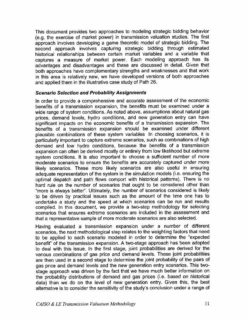
This document provides two approaches to modeling strategic bidding behavior (e.g. the exercise of market power) in transmission valuation studies. The first approach involves developing a game theoretic model of strategic bidding. The second approach involves capturing strategic bidding through estimated historical relationships between certain market variables and a variable that captures a measure of market power. Each modeling approach has its advantages and disadvantages and these are discussed in detail. Given that both approaches have complementary strengths and weaknesses and that work in this area is relatively new, we have developed versions of both approaches and applied them in the illustrative case study of Path 26.
Scenario Selection and Probability Assignments
In order to provide a comprehensive and accurate assessment of the economic benefits of a transmission expansion, the benefits must be examined under a wide range of system conditions. As noted above, assumptions about natural gas prices, demand levels, hydro conditions, and new generation entry can have significant impacts on the economic benefits of a transmission expansion. The benefits of a transmission expansion should be examined under different plausible combinations of these system variables In choosing scenarios, it is particularly important to capture extreme scenarios, such as combrnations of high demand and low hydro conditions, because the benefits of a transmission expansion can often be derived mostly or entirely from low likelrhood but extreme system conditions. It is also important to choose a sufficient number of more moderate scenarios to ensure the benefits are accurately captured under more likely scenarios. These more likely scenarios are also useful in ensuring adequate representation of the system in the simulation models (i.e. ensuring the optimal dispatch and path flows comport with historical patterns). There is no hard rule on the number of scenarios that ought to be consrdered other than “more is always better”. Ultimately, the number of scenarios considered is likely to be driven by practical issues such as the amount of the time one has to undertake a study and the speed at which scenarios can be run and results compiled. In this document, we provide a two-step methodology for selecting scenarios that ensures extreme scenarios are included in the assessment and that a representative sample of more moderate scenarios are also selected.
Having evaluated a transmission expansion under a number of different scenarios, the next methodological step relates to the weighting factors that need to be applied to each scenario modeled in order to determine the “expected benefit” of the transmission expansion. A two-stage approach has been adopted to deal with this issue. In the first stage, joint probabilities are derived for the various combinations of gas price and demand levels. These joint probabilities are then used in a second stage to determine the joint probability of the pairs of gas price and demand levels and the new generation entry scenarios. This two- stage approach was driven by the fact that we have much better information on the probability distributions of demand and gas prices (i.e. based on historical data) than we do on the level of new generation entry. Given this, the best alternative is to consider the sensitivity of the study’s conclusion under a range of
CAISO & LE Transmission Valuatzon Methodology 11
plausible distributions that satisfy certain reasonableness constraints. This can be done through an optimization that chooses, first, a set of joint probabilities of demand, gas price, and new entry scenarios that maximize the expected benefits of a transmission expansion and second, another set of joint probabikties that minimize the expected transmission expansion benefits. This Min-Max optimization approach will then produce a range of potential benefits (lowest to highest) rather than a single expected value. However, it is possible to narrow the range of esttmated benefits by imposing further constraints on the optimization such as requiring that certain scenarios be considered more likely than others.
Measuring Net Benefits
The benefits of a transmission expansion can accrue to both suppliers and consumers and can involve significant welfare transfers between these groups or between locations. Therefore, it is important to measure producer and consumer benefits on a regional basis and to understand how the welfare of these groups shifts under a transmission expansion. For example, a transmission expansion that has a significant Impact on reducrng market power will, for the most part, simply shift welfare from producers to consumers. A conventional social welfare objective in which producer and consumer welfare are given equal weights would show very little net benefit because such a criteria does not consider the distribution effects. It only measures the net effect. However, public policy makers generally do care about distributional effects and therefore benefit measures that reflect the distributional effects are essential to the methodology. This document sets out the principles of cost benefit analysis and provides three benefit measures for policy makers to consider in evaluating a transmission expansion; 1) an approach that gives equal weight to both consumer and producer surplus (i.e. the conventional social welfare objective), 2) an approach that gives equal weight to consumer benefits and the competitive portion of producer benefits (i.e. ignores any benefits that accrue to suppliers from market power), and 3) an approach that only looks at benefits to consumers. Since different decision makers can take different views of the merits of these measures, the most useful output from the transmission valuation methodology will be the building blocks necessary to evaluate the given transmission investment project under all three different objective functions.
An Illustrative Example using Path 26
Various components of this methodology are applied using a proposed expansion of Path 26 as an illustrative case study. However, illustratrve simulations of the estimated benefits of the Path 26 expansion are not provided and will instead be provided prior to the PG&E workshop scheduled for March 14, 2003. It is important to note that the information that will be provided regarding Path 26 does not constitute a definitive assessment of the value from expanding Path 26 rather it will merely serve to demonstrate how the methodology can be carried out and applied in practice. A definitive assessment of Path 26 would require assessing the benefits under more scenarios and
CAISO & LE Transmission Valuation Methodology 12

possibly require a more detailed transmission network representation than was used in this study. Nonetheless, this illustrative case study will demonstrate that the methodology is practical and can produce sensible results.
CAISO & LE Transmission Valuatmn Methodology 13
Introduction Since September 2001, the CAlSO has been working jointly wtth London Economrcs international LLC (LE) to develop a comprehensive methodology for evaluating the economic benefits of transmission investments in a restructured electricity market. In a market oriented restructured environment, a comprehensive approach must address the Impact a transmission expansion would have on market competition and new generation investment. It must also address the inherent uncertainty associated with other critical market drivers such as future hydro conditions, natural gas prices, and demand growth as well as capture the dispatch capability of hydroelectric generation and the availabrlrty of import supplies. This last two factors are particularly critical in modeling the California market given its heavy dependence on hydroelectric generation and imports. Integrating all of these critical modeling requirements into a comprehensive methodological approach is extremely challenging
The methodology presented in the document, which represents the culmination of over a year of joint research between the CAISO and LE with input and review provided by an external steering committee5 and CAISO Market Surveillance Committee, integrates all of these critical modeling requirements into a single comprehensive methodology and demonstrates aspects of the methodology using a proposed expansion of Path 26 as an illustrative case study6. We believe the methodology provided here far exceeds anything that has been done to date in the area of transmission planning studies and that this modeling framework can provide a template for the basic components that a transmission study should address. While much of the focus of this paper is on modeling California transmission projects, the basic approach could be easily adopted to study the benefit of upgrades in other areas of the Western Interconnect.
This paper describes each of the critical components of a comprehensive transmission valuation modeling approach, offers a number of methodological approaches for addressing each of them, and demonstrates aspects of the methodology using a Path 26 expansion as an illustrative case study. The frrst section identifies some important factors one should consider in deciding two fundamental aspects of a transmission study: the transmission network representation and the modeling time horizon. Section II identifies the critical input data for a transmission valuation study such as natural gas prices, demand forecasts, near-term new generation energy, transmission transfer capabilities
5 The external steering commrttee conststed of representattves of the Investor owned utrlrtres (SDG&E, SCE, and PG&E) and various state agencies (CPUC, CEC, and the Electncrty Oversrght Board (EOB)).
6 Varrous components of this methodology are applted ustng a proposed expansron of Path 26 as an rllustratrve case study However, rllustratrve srmulatrons of the estimated benefits of the Path 26 expansron are not provrded and will instead be provrded pnor to the PG&E workshop scheduled for March 14, 2003. It IS Important to note that the rnformatron on the Path 26 expansron wrll be for rllustratrve purposes only. Some lrmited scenarios of a Path 26 expansron are evaluated to demonstrate how the methodology works More scenario analysrs and possrbly a more detarled modal of the transmtssron network would be requrred for a defrmtrve assessment of a Path 26 expansron
CAB0 & LE Transmission Valuation Methodology 14

before and after the expansion, and assumptions about the level of long-term forward energy contracting. The latter is particularly important in assessing the extent to which market power can be exercised. Section Ill provides specific methodologies for critical modeling components. These include assumptions and methodologies for modeling the following components; imports to the CAISO control area, CA hydrology, optimal dispatch of thermal and hydro generation resources, demand price responsiveness, long-term new generatron entry, and market power. To provide a comprehensive and accurate assessment of a transmission expansion, it is critical that the expansion be evaluated under a wide range of system conditions (e.g. demand levels, gas prices, hydro conditions etc.). Section IV provides a methodology for selecting various scenarios of system parameters to ensure a comprehensive and representative set of plausible scenarios. Evaluating the benefits of a transmission expansion under a number of scenarios raises the next methodological issue of how to assign probabilities to these scenarios in order to determine the “expected value” of the project. Section V provides a methodology for assigning probabilities to each of the scenarios. Finally, Section VI provides the basic framework for computing the net-present value of a transmission expansion. The benefits of a transmission expansion can accrue to both consumers and producers. Thus section provides a methodology for calculating the dtfferent benefit components and provides recommendations on the appropriate benefits to consider. A summary of the methodology IS provided in Section VII.
CAB0 & LE Transmission Valuatron Methodology 15
I. Network Representation and Modeling Time Horizon
Transmission Network Representation Perhaps the most fundamental aspect of a transmission study is how one models the transmission network and determines an appropriate modeling time horizon for evaluating the potential benefits of a transmission expansion.
The appropriate scale and scope of the network representation really depends on the type of transmission expansion project being considered. For large transmission projects (e.g. 230 - 500 kV) a broad regional network representation is appropriate since the expansion is likely to have implications throughout the Western Interconnect, particularly in adjacent control areas. When modeling major transmission projects, the need for a detailed network representation is less critical. Moreover, a large overly complex regional model WIII make it more difficult to incorporate critical modeling components such as strategic bidding and may make the model result generally less tractable. The degree of regional network representatron for large transmission projects also depends on the focus of the benefit measures. For example, d the focus of studying a particular large transmission expansion in the CAISO control area IS to measure how such an expansion would benefit California consumers, the need for modeling the major transmission lines outside of the CAISO control area is less critical provided there is adequate representation of the major inter-ties between the CAlSO control area and adjacent control areas. However, as a general matter, a comprehensive assessment should attempt to capture the broader regional benefits and costs of a major transmission expansion, even if the primary interest is in how the expansion benefits California consumers.
Smaller transmrssion expansion projects (e.g. sub-transmission projects at voltage levels less than 230 kV) tend to have more localized benefits, which can be better captured through a more detailed network representation in the electrical vicinity of the project that is more limited in its regional scope. In addition to capturing thermal limrts, smaller projects could also capture local voltage security limits and nomogram constraints7. A detailed network representation for smaller transmission expansions would also allow for evaluating the potential substitutability between reliability must run generation and the transmission expansion.
An import consideration in determining the appropriate level of network detail is ensuring that the model remains tractable. As discussed throughout this document, a comprehensive modeling approach should incorporate many components including modeling long-term new generatton entry and strategic (versus cost-based) bidding behavior. The more complex the network
‘The emphasis here IS on the local nature of voltage security (static) and nomogram constraints. In general, voltage stabMy (dynamic) and system-wlde nomograms should be modeled beyond the local scope
CAB0 & LE Transmission Valuation Methodology 16
representation, in terms of its scope and scale, the more difficult it is to determine whether the model is behaving as expected.
In the illustrative analysis provided in this document, a simplistic network representation was used consisting of the three internal IS0 zones (NP15, ZP26, SP15), the internal paths connecting them (Path 15 and Path 26), and external injections from the Desert Southwest and Pacific Northwest. Because the case study considered here involved the expansion of a major 500 kV line (i.e. expanding Path 26), it was important to model the major importing regions into Calrfornia.
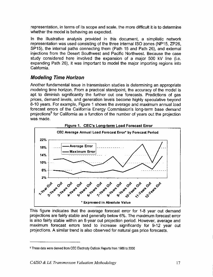
Modeling Time Horizon Another fundamental issue in transmission studies is determining an appropriate modelrng time horizon. From a practical standpoint, the accuracy of the model is apt to diminish significantly the further out one forecasts. Predictions of gas prices, demand levels, and generation levels become highly speculative beyond 8-10 years. For example, Figure 1 shows the average and maximum annual load forecast errors of the California Energy Commission’s long-term base demand projections’ for California as a function of the number of years out the projection was made.
Figure 1. CEC’s Long-term Load Forecast Error
CEC Average Annual Load Forecast Error* by Forecast Period
l Expressed in Absolute Value ,.
This tigure indicates that the average forecast error for 1-8 year out demand projections are fairly stable and generally below 6%. The maximum forecast error is also fairly stable within an 8-year out projection period. However, average and maximum forecast errors tend to increase significantly for 9-12 year out projections. A similar trend is also observed for natural gas price forecasts.
8 These data were dewed from CEC Electwty Outlook Repolts from 1988 to 2000
CAISO & LE Transm~ssron Valuation Methodology 17

Because the accuracy of the base-line input assumptions used in the model is apt to diminish significantly for projections out beyond &years, it is critical that the benefits of the transmission expansion be evaluated under a number of different input assumptions (i.e. scenarios). Assessing the benefits under a variety of input assumptions can compensate for the inherent uncertainty of these parameters and allow for the estimation of a reasonable range of expected values.
In determining a study period, one needs to also consider when the transmission expansion can be completed. Most transmissron projects typically take several years to complete. Given this, if one establishes a 13-year study period with the first year being the current year, the first several years will not produce any benefits or costs srnce the project would not be on-line until several years out. However, modeling the first few years is still a good practice as it will help to calibrate the model. The initial years prior to expansion can also serve as a benchmark for the net benefit analysis in that tf the model is functioning appropriately it should produce zero net-benefits in these years,
Given these considerations, a study period in the range of 12-15 years, beginning with the next full calendar year is a reasonable time horizon for a transmrssion study. Benefit estimates beyond this range would be highly speculative due to the uncertainty of future system conditions. Assuming an average transmission development time of 6 years, a time horizon of 12-15 years would provide 6-9 years of annual benefit estimates. However, a shorter time horizon can be appropriate, if a transmission project can be shown to be economically viable within the shorter time frame.
CAISO & LE Transmzsslon Valuation Methodology 18

II. Critical Input Components
Modeling Gas Prices Fuel price variation can have a material impact on the benefits of transmission because the CAISO system comprises different technologies and different regional distribution of those technologies. Changing relative fuel prices can be expected to change the relative short-run costs of these technologies which, in some cases, may result in changed patterns of utikzatron. The changes in utilrzation will be affected by transmission capacity. Hence, for example:
1. The incremental heat rates of gas fired units are highly non-linear and vary significantly depending on whether the unit is a base load combined cycle or a peaking CT (i.e. combustion turbine) unit. Because of the non-linearity of the incremental heat rates, assuming a different gas price can have a significant impact on the price differentials of the no-expansion and expansion scenarios.
2. If units are dispatched based on a daily commitment process, a higher gas price may result in more base-load units being committed rather than dispatching CTs.
3. Higher gas prices may result in more hydroelectric generation being dispatched.
Furthermore, the relativity of producer and consumer surplus is directly affected by changes in relative fuel prices; thus, depending on the choice of objective function, fuel price assumptions can significantly change the magnitude and distribution of social welfare. Therefore, rt is important to assess the benefits of a transmission expansion under a number of plausible gas price scenarios and to capture potential regional variations in gas prices
In the illustrative analysis of Path 26, base-line gas price forecasts for 2002-2014 were derived from the CEC’s June 2002 unpublished forecast of annual natural gas prices and monthly natural gas price multipliers, which was very similar to that published in CEC’s 2002-2012 Electricity Outlook Repoti, February 2002. These forecasts are on an all-in delievered cost basis (burner tip) to electric generators in 2000 dollar terms. We have converted the CEC forecast to 2002 dollar terms, using the deflation index provided by the CEC in their 2002-2012 Electricity Outlook Report. Due to the similarity in the SoCal Gas and SDG&E forecasts, we decided to use SoCal Gas price forecasts for gas-fired generation in the SP15 zone and the PG&E gas price forecasts for gas-fired generation in the NP15 region.
CAB0 & LE Transmission Valuation Methodology 19
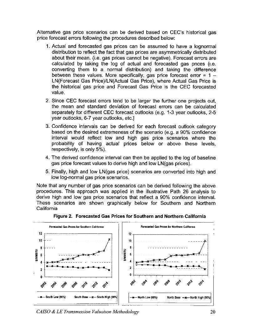
Alternative gas price scenarios can be derived based on CEC’s historical gas price forecast errors following the procedures described below:
1. Actual and forecasted gas prices can be assumed to have a lognormal distribution to reflect the fact that gas prices are asymmetrically distributed about their mean. (i.e. gas prices cannot be negative). Forecast errors are calculated by taking the log of actual and forecasted gas prices (I.e. converting them to a normal distribution) and taking the difference between these values. More specifically, gas price forecast error = 1 - LN(Forecast Gas Price)/LN(Actual Gas Price), where Actual Gas Price is the historical gas price and Forecast Gas Price is the CEC forecasted value.
2. Since CEC forecast errors tend to be larger the further one projects out, the mean and standard deviation of forecast errors can be calculated separately for different CEC forecast outlooks (e.g. 1-3 year outlooks, 2-5 year outlooks, 6-7 year outlooks, etc.]
3. Confidence intervals can be derived for each forecast outlook category based on the desired extremeness of the scenario (e.g. a 90% confidence interval would reflect low and high gas price scenarios where the probability of having actual prices below or above these levels, respectively, is only 5%).
4. The derived confidence interval can then be applied to the log of baseline gas price forecast values to derive high and low LN(gas prices).
5. Finally, high and low LN(gas price) scenarios are converted into high and low log-normal gas price scenarios.
Note that any number of gas price scenarios can be derived following the above procedures. This approach was applied in the illustrative Path 26 analysis to derive high and low gas price scenarios that reflect a 90% confidence interval. These scenarios are shown graphically below for Southern and Northern California
Figure 2. Forecasted Gas Prices for Southern and Northern California
CAISO & LE Transmmion Valuatron Methodology 20
Modeling Demand Forecasts Forecasted demand levels can have significant impacts on the benefit results. Generally speaking, the higher the demand in the importing zone of a constrained transmission Interface, the greater the benefit of the expansion. Demand levels Impact the benefit of a transmission project in several respects.
1.
2.
3.
Higher demand levels will result in higher cost resources being dispatched and extremely hrgh demand levels may also result in the dispatch of curtailable load, which, depending on how curtailable load is modeled, can have a significant Impact on the price forecast results.
Higher demand levels will tend to increase market power. The ability of a supplier to exercise market power depends largely on the degree to whrch the supplier is “pivotal” in the sense that demand could not be met absent the supplier’s capacity. In general, higher demand levels result in suppliers being more pivotal and thus being better able to exercise market power.
Since the benefits of transmission project are typically measured by changes in producer and/or consumer surplus and both of these measures are based on the amount of load served, the assumed level of load will have a significant multiplier effect on the estimated social benefits.
Given these impacts, it is important to utilize the best available forecasts on future demand levels and to conduct multiple modeling runs under different demand scenarios to capture the uncertainty.
In the illustrative Path 26 analysis, base-line demand forecasts for 2002-2014 were derived from the CEC’s long-term base demand projection published in CEC’s 2002-2072 Necfricity Outlook Report CEC derived its baseline scenario of demand forecasts for 2002-2012 under the following three assumptions:
a) Annual average energy consumption forecast based on normal economic growth trends in the 2002-2012 period;’
b) Annual statewide peak demand forecast based on temperature conditions that have a l-in-2 probability of occurring; and
c) A 50% probability of persistence of 2001 demand reduction effect.
Demand forecasts for 2013 and 2014 were calculated by linearly extrapolating the CEC’s 2012 growth rate forecast for both peak demand and energy consumption. This approach yielded base demand cases that assume a 1.9% average annual growth over forecast time horizon in peak demand and total energy The resulting annual peak demand and energy consumption figures, along with the CEC’s target assumption on levels of conservation, was applied to
9 The normal economic growth trend does not Include the economic downturn I” 2001 or any of the effect of the September liti, 2001 tragedy
CAISO & LE Transmission Valuation Methodology 21
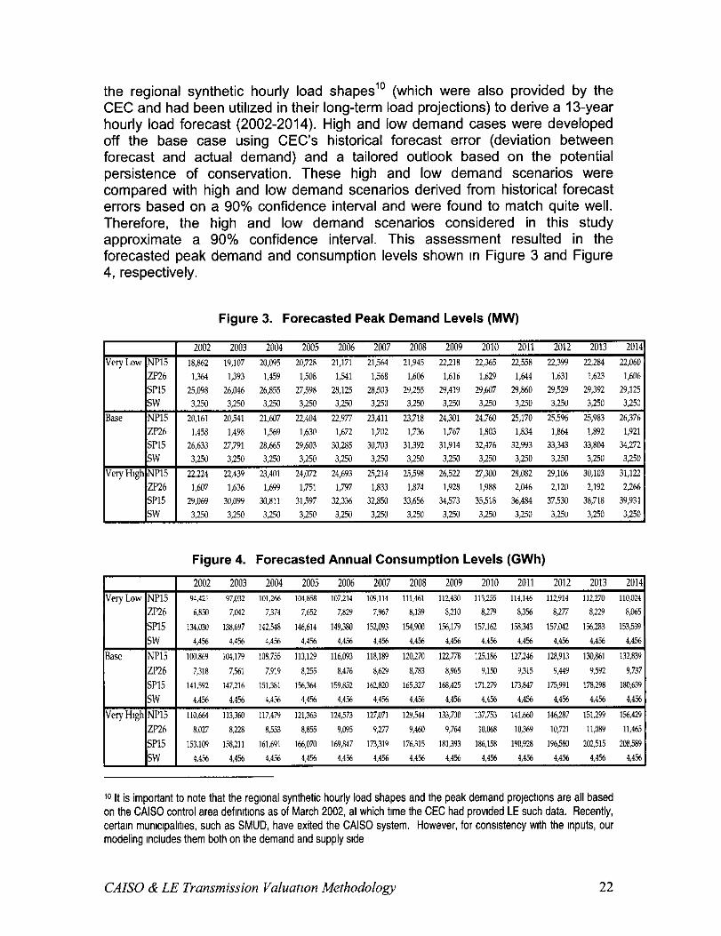
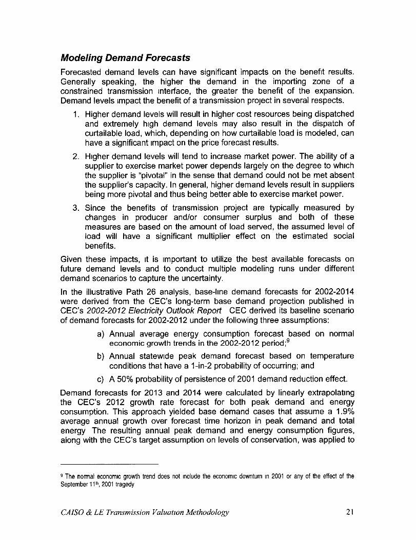
the regional synthetic hourly load shapes” (which were also provided by the CEC and had been utikzed in their long-term load projections) to derive a 13-year hourly load forecast (2002-2014). High and low demand cases were developed off the base case using CEC’s historical forecast error (deviation between forecast and actual demand) and a tailored outlook based on the potential persistence of conservation. These high and low demand scenarios were compared with high and low demand scenarios derived from historical forecast errors based on a 90% confidence interval and were found to match quite well. Therefore, the high and low demand scenarios considered in this study approximate a 90% confidence interval. This assessment resulted in the forecasted peak demand and consumption levels shown In Figure 3 and Figure 4, respectively.
Figure 3. Forecasted Peak Demand Levels (MW)
2002 2003 2004 2005 2006 2w7 2008 2009 2010 2011 2012 2013 2014 Very Low NP15 18,862 19,107 20,095 20,728 21,171 21,561 21,945 22218 22,355 22,558 22,399 22284 22,060
ZP26 1,364 1,393 1,459 1,508 1,541 1,568 1,606 1,616 1,629 I.614 1,631 1,623 1,606 SF15 25,098 26,046 26,855 27,598 28,125 28,503 29,255 29,419 29,647 29,860 29.529 29,392 29,125 SW 3,250 3,250 3,250 3250 3,250 3,250 3,250 3,250 3m 3,250 3,250 3,250 3250
B‘W NPl5 20,161 20,541 21,607 22,404 22.977 23,411 23,718 24,m 24,760 25,170 23.5% 25,983 26,376 ZF-26 1,458 1,498 1,569 1,630 1,672 1,702 1,736 1,767 1,803 1,834 1,864 1,892 1,921 SPl5 26,633 27,791 Z&M5 29,603 30,285 30,703 31,392 31,914 32,476 32,993 33,343 33,804 34,272 lsw 1 3,250 3,250 3,250 3,250 3,250 3250 3,250 3,250 3,250 3,250 3.250 3,230 3,250
VeryH1~hlNP15 I 22,224 22,439 23,401 24,072 24,693 25,214 25,598 26,522 27,300 28,082 29,106 30,103 31,122 _ ZF26 1,607 1,636 1,699 1,751 1,797 1,833 1,874 1,928 1,988 2,046 2,120 2,192 2,266 SP15 29,069 30,099 30,811 31,597 32,336 32.850 33,656 34,573 35,518 36,481 37.530 38,718 39,931 SW 3,250 3,250 3,250 3,250 3,250 3,250 3,250 3,250 3250 3,250 3,250 3,250 3,250
Figure 4. Forecasted Annual Consumption Levels (GWh)
2002 2003 2004 2005 2006 2007 2008 2009 2010 2011 2012 2013 2014 very Low NP15 91,121 97,012 101ZM mm8 107,214 109,119 lll,Ml 112,430 111,255 11w6 112,911 11wo 110.024
ZP26 6,859 7,w 7,374 7,652 7,829 7,967 8,139 8,210 8,279 8.3% 8,277 8,229 8,065 315 E4,ow 138,697 142.M 146,614 149,380 152,cm 154,900 156,179 157,162 lwd3 157,@42 155,283 153,539
10 It is important to note that the regtonal synthetic hourly load shapes and the peak demand prolectlons are all based on the CAISO control area deflmtlons as of March 2002, at which time the CEC had prouded LE such data. Recently, certain munupalltles, such as SMUD, have exited the CAISO system. However, for consistency with the Inputs, our modeling Includes them both on the demand and supply side
CAISO & LE Transmission Valuatzon Methodology 22
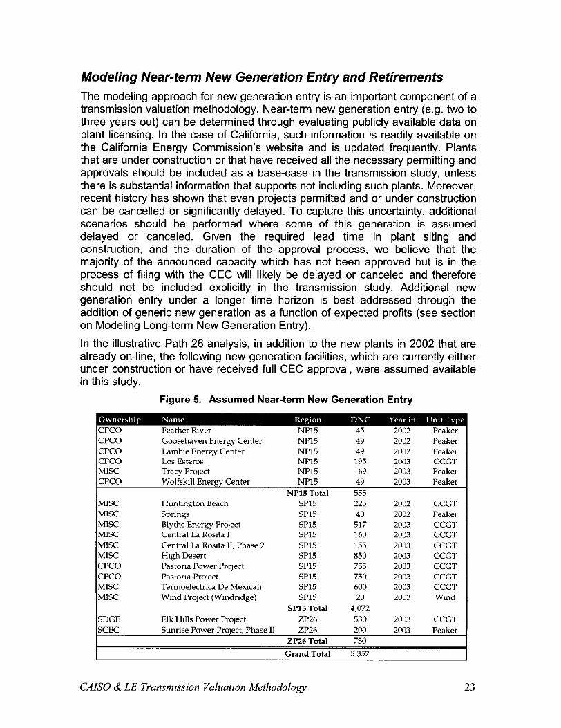
Modeling Near-term New Generation Entry and Retirements The modeling approach for new generation entry is an important component of a transmission valuation methodology. Near-term new generation entry (e.g. two to three years out) can be determined through evaluating publicly available data on plant licensing. In the case of California, such information is readily available on the California Energy Commission’s website and is updated frequently. Plants that are under construction or that have received all the necessary permitting and approvals should be included as a base-case in the transmrssion study, unless there is substantial information that supports not including such plants. Moreover, recent history has shown that even projects permitted and or under construction can be cancelled or significantly delayed. To capture this uncertainty, additional scenarios should be performed where some of this generation is assumed delayed or canceled. Grven the required lead time in plant siting and construction, and the duration of the approval process, we believe that the majority of the announced capacity which has not been approved but is in the process of filing with the CEC will likely be delayed or canceled and therefore should not be included explicitly in the transmission study. Additional new generation entry under a longer time horizon IS best addressed through the addition of generic new generation as a function of expected profits (see section on Modeling Long-term New Generation Entry).
In the illustrative Path 26 analysis, in addition to the new plants in 2002 that are already on-line, the following new generation facilities, which are currently either under construction or have received full CEC approval, were assumed available in this study.
Figure 5. Assumed Near-term New Generation Entry
Lamble Energy Center Los Esteros
NP15 NP15
49 195
2002 2003
Faker CCGT
Blythe Energy I’rqect Central La Roslta I Central La Roslta II, Phase 2 H,gh Desert Pastona Power ProJect Pastorla Prqect Termoelectnca De Mexxah Wmd Prqect (Wmdndge)
SF15 SP15 SP15 SF15 SP15 SF15 SF15 SP15 SF15 SF15
225 40
517 160 155 850 755 750 600 20
2002 2002 2003 2003 2003 2003 2003 2003 2003 2003
CCGT Peaker CCGT CCGT CCGT CCGT CCGT CCGT CCGT Wmd
CAISO & LE Transmrssion Valuation Methodology 23
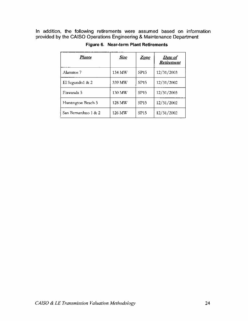
In addition, the following retirements were assumed based on information provided by the CAL’30 Operations Engineering & Maintenance Department
Figure 6. Near-term Plant Retirements
I plants I
Alamtos 7 134 Am’ SP15
El Segundo1 & 2 339 Mw SPlj
Euwanda 5 130 Mw SP15
Huntington Beach 5 128 MY7 SP15
San Bemardmo 1 & 2 126 MW SP15
Size -
CAISO & LE Transmission Valuation Methodology 24
mf Retirement
12/31/2003
12/31/2002
12/31/2003
12/31/2002
12/31/2002
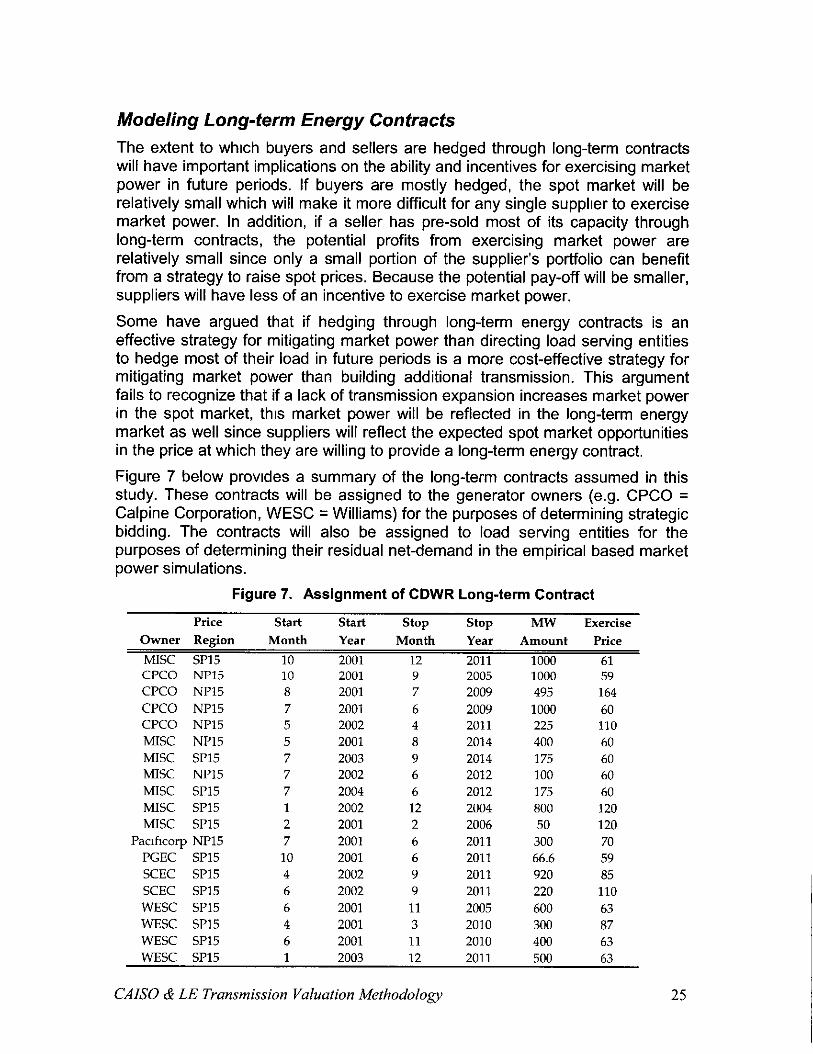
Modeling Long-term Energy Contracts The extent to which buyers and sellers are hedged through long-term contracts will have important implications on the ability and incentives for exercising market power in future periods. If buyers are mostly hedged, the spot market will be relatively small which will make it more difficult for any single suppker to exercise market power. In addition, if a seller has pre-sold most of its capacity through long-term contracts, the potential profits from exercising market power are relatively small since only a small portion of the supplier’s portfolio can benefit from a strategy to raise spot prices. Because the potential pay-off will be smaller, suppliers will have less of an incentive to exercise market power.
Some have argued that if hedging through long-term energy contracts is an effective strategy for mitigating market power than directing load serving entities to hedge most of their load in future periods is a more cost-effective strategy for mitigating market power than building additional transmission. This argument fails to recognize that if a lack of transmission expansion increases market power in the spot market, thus market power will be reflected in the long-term energy market as well since suppliers will reflect the expected spot market opportunities in the price at which they are willing to provide a long-term energy contract.
Figure 7 below provrdes a summary of the long-term contracts assumed in this study. These contracts will be assigned to the generator owners (e.g. CPCO = Calpine Corporation, WESC = Williams) for the purposes of determining strategic bidding. The contracts will also be assigned to load serving entities for the purposes of determining their residual net-demand in the empirical based market power simulations.
Figure 7. Assignment of CDWR Long-term Contract
Price start start stop stop MW Exercise Owner Region
MISC SP15
Month
10
Year 2001
Month 12
YeEN Amount Price
2011 1000 61 CI’CO NP15 10 2001 9 2005 1000 59 CPCO NP15 8 2001 7 2009 495 164 CPCO Nl’15 7 2001 6 2009 1000 60 CPCO NP15 5 2002 4 2011 225 110 MISC NP15 5 2001 8 2014 400 60 MISC SF15 7 2003 9 2014 175 60 MISC NP15 7 2002 6 2012 100 60 MISC SP15 7 2004 6 2012 175 60 Mlsc SP15 1 2002 12 2004 800 120 MISC SF15 2 2001 2 2006 50 120
Paaficorp Nl’15 7 2001 6 2011 300 70 PGEC SP15 10 2001 6 2011 66.6 59 SCEC SP15 4 2002 9 2011 920 85 SCEC SP15 6 2002 9 2011 220 110 WESC SP15 6 2001 11 2005 600 63 WESC SP15 4 2001 3 2010 300 87 WESC SP15 6 2001 11 2010 400 63 WESC SP15 1 2003 12 2011 500 63
CAISO & LE Transmission Valuation Methodology 25
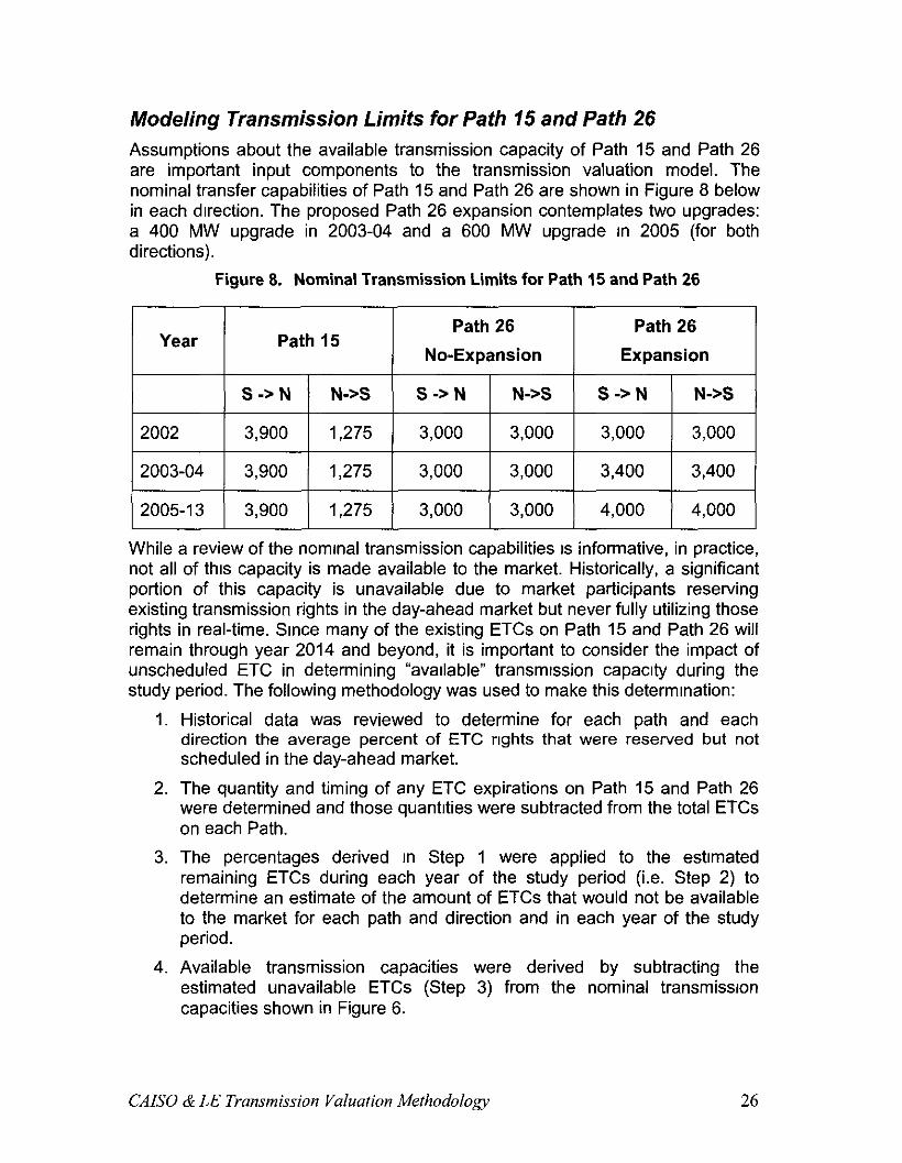
Modeling Transmission Limits for Path 15 and Path 26 Assumptions about the available transmission capacity of Path 15 and Path 26 are important input components to the transmission valuation model. The nominal transfer capabilities of Path 15 and Path 26 are shown in Figure 8 below in each drrection. The proposed Path 26 expansion contemplates two upgrades: a 400 MW upgrade in 2003-04 and a 600 MW upgrade In 2005 (for both directions).
Figure 8. Nominal Transmission Limits for Path 15 and Path 26
Year Path 15 Path 26
No-Expansion
Path 26
Expansion I
S -> N N-S S -> N N-S S -> N N-Xii
2002 3,900 1,275 3,000 3,000 3,000 3,000
2003-04 3,900 1,275 3,000 3,000 3,400 3,400
2005-I 3 3,900 1,275 3,000 3,000 4,000 4,000
While a review of the nominal transmission capabilities IS informative, in practice, not all of thus capacity is made available to the market. Historically, a significant portion of this capacity is unavailable due to market participants reserving existing transmission rights in the day-ahead market but never fully utilizing those rights in real-time. Srnce many of the existing ETCs on Path 15 and Path 26 will remain through year 2014 and beyond, it is important to consider the impact of unscheduled ETC in determining “available” transmission capacity during the study period. The following methodology was used to make this determination:
1. Historical data was reviewed to determine for each path and each direction the average percent of ETC rights that were reserved but not scheduled in the day-ahead market.
2. The quantity and timing of any ETC expirations on Path 15 and Path 26 were determined and those quantities were subtracted from the total ETCs on each Path.
3. The percentages derived in Step 1 were applied to the estimated remaining ETCs during each year of the study period (i.e. Step 2) to determine an estimate of the amount of ETCs that would not be available to the market for each path and direction and in each year of the study period.
4. Available transmission capacities were derived by subtracting the estimated unavailable ETCs (Step 3) from the nominal transmissron capacities shown in Figure 6.
CAB0 & LE Transmission Valuation Methodology 26
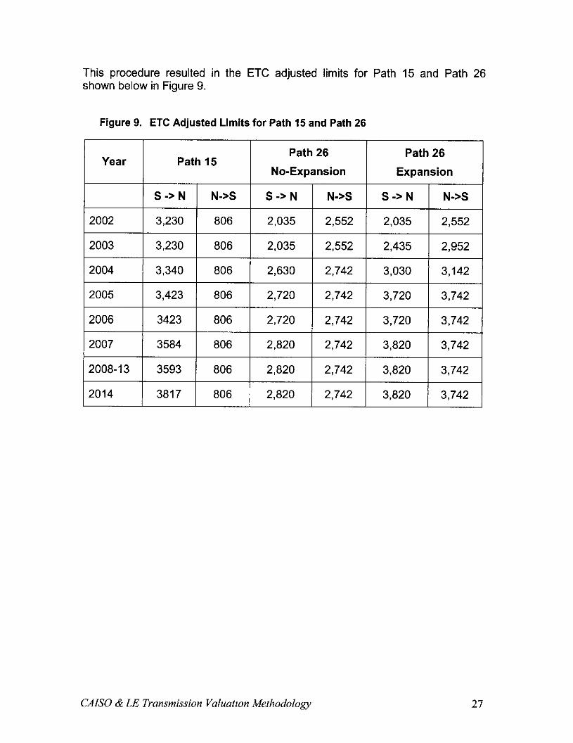
This procedure resulted in the ETC adjusted limits for Path 15 and Path 26 shown below in Figure 9.
Figure 9. ETC Adjusted Limits for Path 15 and Path 26
Year Path 15 Path 26
No-Expansion
Path 26
Expansion 1
S -> N N-S S -> N N-S S -> N N-S
2002 3,230 806 2,035 2,552 2,035 2,552
2003 1 3,230 1 806 1 2,035 1 2,552 I 2,435 1 2,952
2004 3,340 806 2,630 2,742 3,030 3,142
2005 3,423 806 2,720 2,742 3,720 3,742
2006 3423 806 2,720 2,742 3,720 3,742
2007 3584 806 2,820 2,742 3,820 3,742
2008-I 3 3593 806 2,820 2,742 3,820 3,742
2014 3817 806 2,820 2,742 3,820 3,742
CAISO & LE Transmission Valuation Methodology 27
III. Critical Modeling Components
Modeling /mports When modeling the benefits of a major transmission expansion within the CAlSO control area, it is Important to have a good representation of the availability and cost of import supplies from both the Desert Southwest and the Pacific Northwest so that these supply sources can be incorporated into the optimal dispatch. Ideally the network representation used for evaluating a major transmission project within the CAlSO control area would include a representation of significant generation, transmissron, and load resources outsrde the IS0 control area. The representation does not need to be extremely detailed but should instead capture the major load areas, generation resources, and transmrssion constraints. These components would be integrated into a regional model and the dispatch algorithm would minimize production cost for the entire region. However, acquiring the necessary data to develop such a regional model and the calibration of that model would be a significant undertaking. One would need cost information on major power plants, the capacity values of major hydro resources, regional load forecasts, and anticipated new power plants throughout the WECC interconnect. If one were to obtain all the necessary data and incorporate into a regional dispatch model, extensive testing would be necessary to ensure the model is producing results consistent with observed historical patterns. One area that would be extremely challenging is calibrating the dispatch of hydroelectric resources in the Pacific Northwest. For example, environmental and alternative use constraints on the utilization of hydro resources in the Pacific Northwest would be difficult to incorporate into the modeling process.
The difficulties in developing a broad regional model are not insurmountable - indeed, commercial models exist that do this - but the incorporation of the wider WECC representation into the strategic bidding representations used in this analysis would require a collaborative effort between all the major control areas that comprise the WECC interconnect. In the interim, it will be necessary to adopt a more stylized representation of external areas From California’s standpoint, there are two major importing regions, the Pacific Northwest and the Desert Southwest, both of which have very different characteristics that must be reflected in their representation, The Pacific Northwest load is greatest during the winter months and its generation base is almost entirely hydroelectric. The implications of this to California is that imports from the Pacific Northwest are greatest in the late Spring and Summer but diminish significantly through the Fall and Winter. Other important implications to California are that summer availabilrty of Pacific Northwest imports can vary dramatically depending on the overall hydro storage and snow pack conditions.
The availability of imports to California from the Desert Southwest has very different characteristrcs. In the Desert Southwest seasonal demand patterns tend to coincide with California’s seasonal demand and the generation base in the Desert Southwest is largely thermal The implications of this to California is that
CAB0 & LE Transmission Valuatton Methodology 28
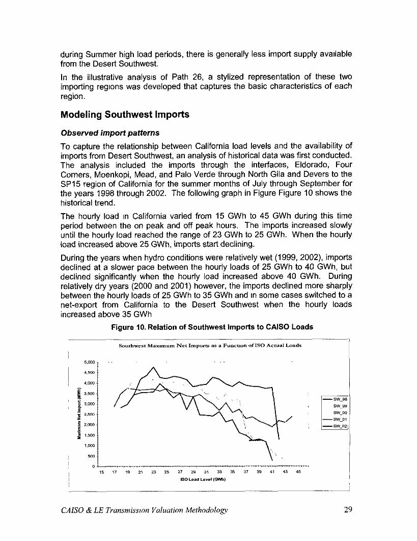
during Summer high load periods, there is generally less import supply avarlable from the Desert Southwest.
In the illustrative analysrs of Path 26, a stylized representation of these two importing regrons was developed that captures the basic characteristics of each region.
Modeling Southwest Imports
Observed import patterns
To capture the relationship between California load levels and the availability of imports from Desert Southwest, an analysis of historical data was first conducted. The analysis included the imports through the interfaces, Eldorado, Four Corners, Moenkopi, Mead, and Palo Verde through North Gila and Devers to the SP15 region of California for the summer months of July through September for the years 1998 through 2002. The following graph in Figure Figure 10 shows the historical trend.
The hourly load In California varied from 15 GWh to 45 GWh during this time period between the on peak and off peak hours. The imports increased slowly until the hourly load reached the range of 23 GWh to 25 GWh. When the hourly load increased above 25 GWh, imports start declining.
During the years when hydro conditions were relatively wet (1999, 2002) imports declined at a slower pace between the hourly loads of 25 GWh to 40 GWh, but declined significantly when the hourly load increased above 40 GWh. During relatively dry years (2000 and 2001) however, the imports declined more sharply between the hourly loads of 25 GWh to 35 GWh and in some cases switched to a net-export from California to the Desert Southwest when the hourly loads increased above 35 GWh
Figure 10. Relation of Southwest Imports to CAISO Loads
CAISO & LE Transmissxm Valuation Methodology 29
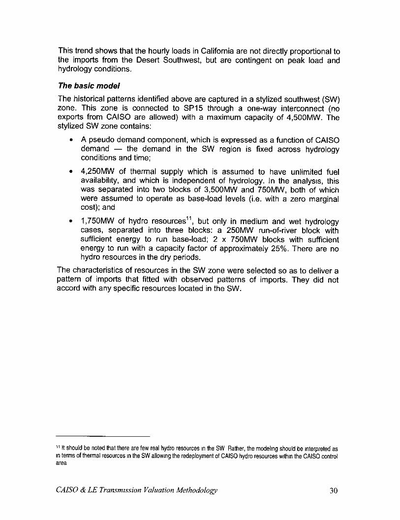
This trend shows that the hourly loads in California are not directly proportional to the imports from the Desert Southwest, but are contingent on peak load and hydrology conditions.
The basic model
The historical patterns identified above are captured in a stylized southwest (SW) zone. This zone is connected to SP15 through a one-way interconnect (no exports from CAlSO are allowed) with a maximum capacity of 4,500MW. The stylized SW zone contains:
. A pseudo demand component, which is expressed as a function of CAISO demand - the demand in the SW region is fixed across hydrology conditions and time;
l 4,250MW of thermal supply which is assumed to have unlimited fuel availabikty, and which is independent of hydrology. In the analysts, this was separated into two blocks of 3,500MW and 750MW, both of which were assumed to operate as base-load levels (i.e. with a zero marginal cost); and
l 1,750MW of hydro resources”, but only in medium and wet hydrology cases, separated into three blocks: a 250MW run-of-river block with sufficient energy to run base-load; 2 x 750MW blocks with sufficient energy to run with a capacity factor of approximately 25%. There are no hydro resources in the dry periods.
The characteristics of resources in the SW zone were selected so as to deliver a pattern of imports that fitted with observed patterns of imports. They did not accord with any specific resources located in the SW.
j1 It should be noted that there are few real hydm resources in the SW Rather, the modeltng should be Interpreted as in terms of thermal resources in the SW allowlng the redeployment of CAlSO hydro resources wlthln the CAlSO control area
CAB0 & LE Transmssion Valuation Methodology 30
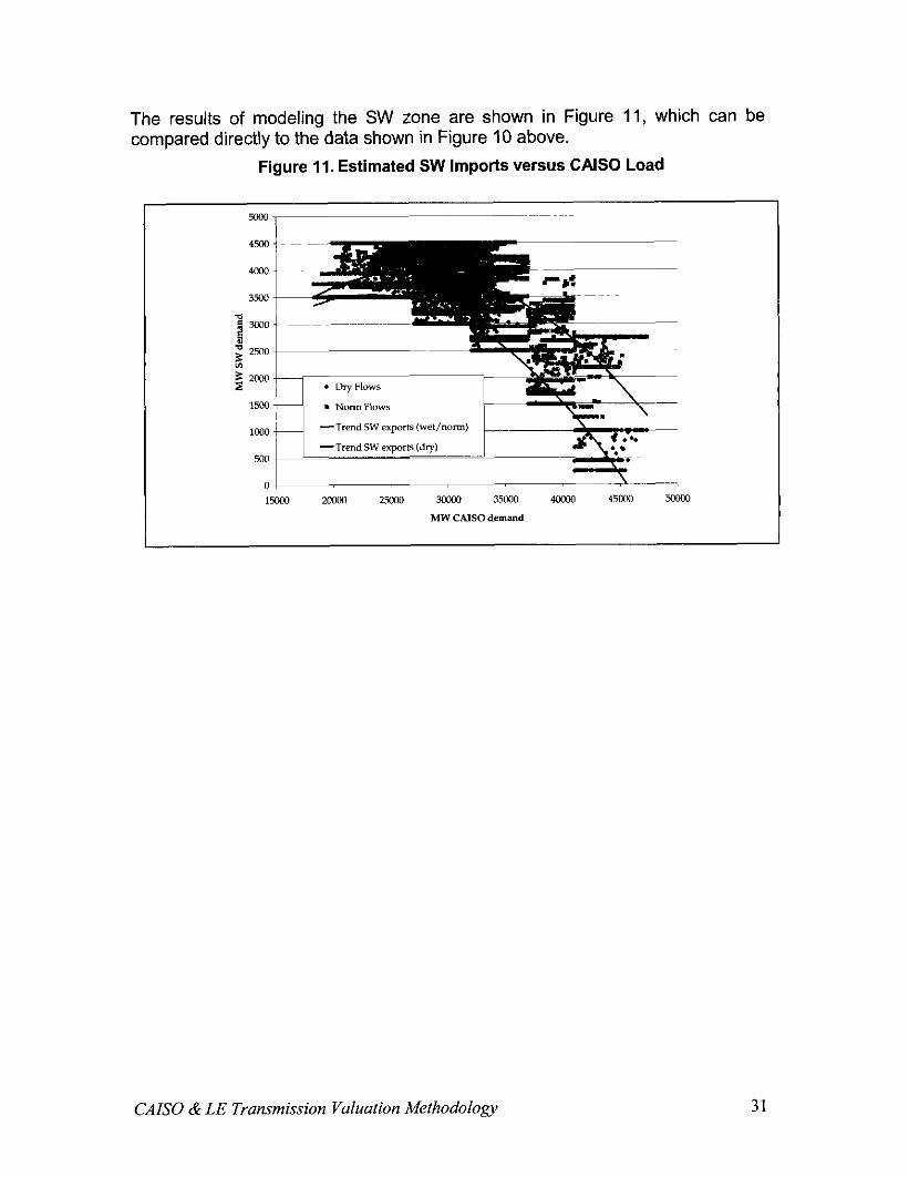
The results of modeling the SW zone are shown in Figure 11, which can be compared directly to the data shown in Figure 10 above.
Figure 11. Estimated SW Imports versus CA60 Load
CAISO & LE Transmission Valuation Methodology 31
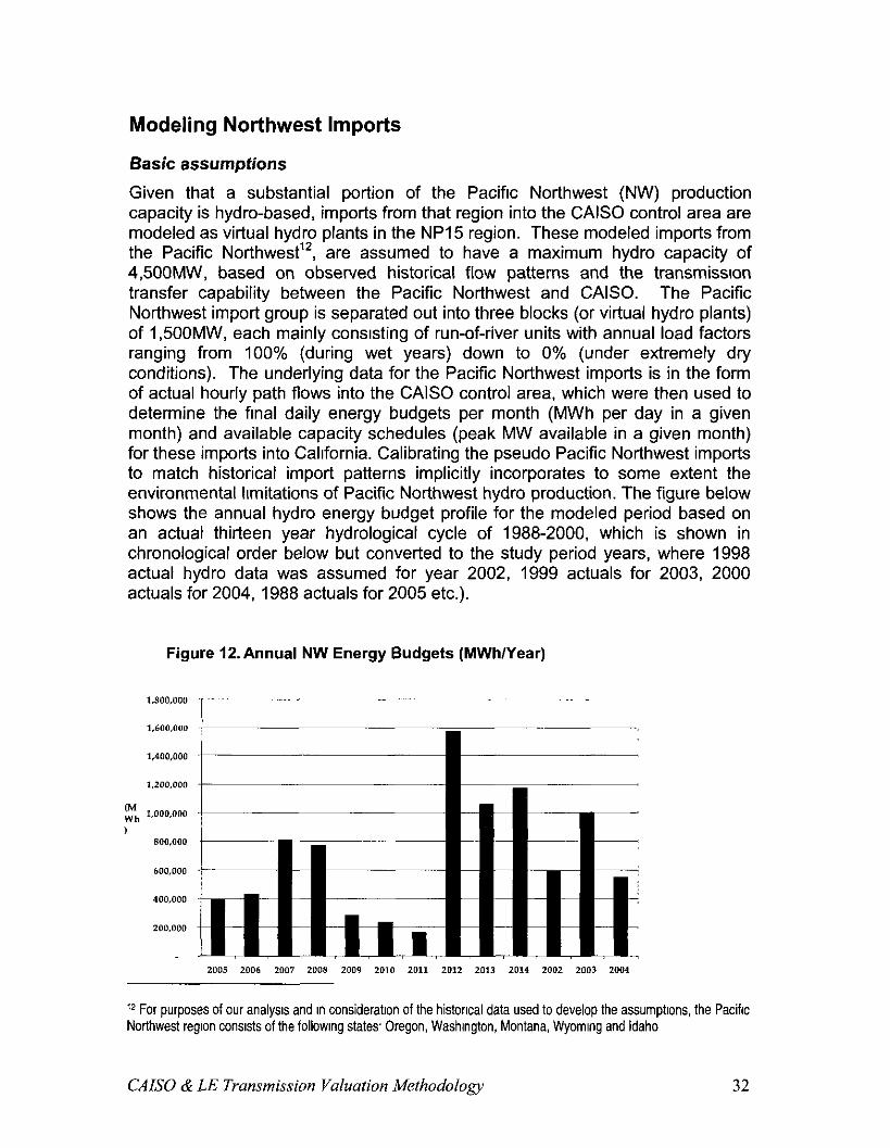
Modeling Northwest Imports
Basic assumptions
Given that a substantial portion of the Pacific Northwest (NW) production capacity is hydro-based, imports from that region into the CAlSO control area are modeled as virtual hydro plants in the NP15 region. These modeled imports from the Pacific Northwest”, are assumed to have a maximum hydro capacity of 4,5OOMW, based on observed historical flow patterns and the transmissron transfer capability between the Pacific Northwest and CAISO. The Pacific Northwest import group is separated out into three blocks (or virtual hydro plants) of 1,50OMW, each mainly consrsting of run-of-river units with annual load factors ranging from 100% (during wet years) down to 0% (under extremely dry conditions). The underlying data for the Pacific Northwest imports is in the form of actual hourly path flows into the CAISO control area, which were then used to determine the frnal daily energy budgets per month (MWh per day in a given month) and available capacity schedules (peak MW available in a given month) for these imports into California. Calibrating the pseudo Pacific Northwest imports to match historical import patterns implicitly incorporates to some extent the environmental limitations of Pacific Northwest hydro production. The figure below shows the annual hydro energy budget profile for the modeled period based on an actual thirteen year hydrological cycle of 1988-2000, which is shown in chronological order below but converted to the study period years, where 1998 actual hydro data was assumed for year 2002, 1999 actuals for 2003, 2000 actuals for 2004, 1988 actuals for 2005 etc.).
un e 12.Annual NW Energy Budgets (MWh/Year)
t -.
I
I2 For purposes of our analysrs and In consideration of the historlcal data used to develop the assumptrons, the Pacific Northwest regron consrsts of the followrng states Oregon, WashIngton, Montana, Wyoming and Idaho
CAISO & LE Transmission Valuation Methodology 32
In Figure 12, 1998 (shown as 2002) was selected as the starting point for the 13- year hydro cycle because It was determined that the historical hydro production for 1998-2000 would most closely match expected hydro conditions in 2002- 2004, as we discuss further below on ‘Modeling California Hydrology’. The 13- year series covers 1988-2000 rather than 1990-2002 because the analysis originally began in the Fall of 2001 and there was not sufficient time to update the analysis to the most recent 13-year hydro cycle (i.e. 1990-2002).
The maximum committable level of NW hydro capacity to California is dependent upon observed annual hydro conditions (i.e. wet, dry or medium) using a similar methodology as that which was used to develop the hydro generation schedules for those plants internal to the California IS0 control region (see next section). Each years hydrology profile is sculpted into month-specific daily energy budgets to reflect the historically observed monthly profile of NW imports, but thereafter committed and drspatched in the same way as hydro resources located wrthin NP15. The maximum output from these pseudo NW resources was set by reference to import constraints from the NW. Exports from the California IS0 to the Pacific Northwest are included as a portion of the total projected demand for the NP15 region, based on the stylized representation of flows in the transportation model (i.e., this approach basically assumes that all the export capacity flows directly from the NP15 region, though in reality, some exports from the South (SP15 and other control areas south of Path 15) can occur through the Pacific DC Intertie) I3
I3 It should also be noted that at times these exports from CAB0 to the NW can be curtaIled The ablllty to curtall exports in this manner was represented through notlonal generatlon resources I” the CAB0 termed ‘export release’ resources
CAB0 & LE Transmission Valuation Methodology 33
Modeling California Hydrology How one models the availability of hydroelectric generation within California can have important implications on the model results. A methodology for modeling hydroelectric generation must recognize that these resources are typically energy limited (i.e. energy production is limited by the availability of water) and as a consequence, the optimal dispatch must reflect inter-temporal opportunity costs (i.e. the cost of the energy produced today should reflect the foregone market opportunity of selling that energy in some future period). An opportunity cost approach to drspatching hydroelectric supply will optimize the value of hydroelectric production by dispatching it in the highest priced periods. In modeling hydroelectric dispatch one must also recognize the maximum production capabilities of these resources in any particular hour often depends on the overall hydrology conditions. In very dry years, the maximum hourly productron capabilities of some facilities is limited due to a lack of river flow or pond storage conditions. This section describes a methodology for matching the maximum output of hydroelectric resources with overall hydrology condrtions. The methodology for optimally dispatching California hydroelectric resources is described in the next sectron.
The underlying data for the Californra hydrology assumptions came from CEC historical hydro monthly output data (1984-2000). This publicly-available data set was used as the basis for the construction of the 13-year California hydro scenario. This data set comprises actual monthly hydro generation output on a per unit basis, along with the nameplate capacities for each unit. Plant capacity data was cross-referenced with data from the EIA and FERC Form 1 for certain plants, in order to identify and correct any inconsistency in the data or clarify ambivalent capacities in the CEC database.
The hydrology data was also benchmarked against actual metered production figures compiled by the CAISO from the last few years of operation. The simulation model used in this analysis seeks to optimize the use of hydro resources by schedukng its use for peak periods where prices are expected to be highest. The results of the simulation studies and, in consequence, the benefits of a transmission expansion are highly sensitive to assumptions on the ability of NP15 hydro resources to schedule their production in this way. The initial modeling allowed hydro resources to schedule to their maximum capacities (their published PMM figures), but this was found to give patterns of use substantially different from observed patterns, and patterns of transmission use that differed from observed patterns. After several iterations of the modeling, more realisticI outcomes were achieved by adjusting hydro peak capacity by their monthly energy availability.
I4 In the sense that the ‘more reaktc modeltng parameters gave a pattern of transmlsslon flows and hydro use that most closely matched actual htstoncal observations
CAISO & LE Transmission Valuation Methodology 34
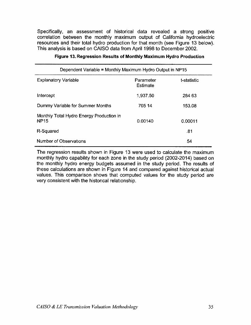
Specifically, an assessment of historical data revealed a strong positive correlation between the monthly maximum output of California hydroelectric resources and their total hydro production for that month (see Figure 13 below). This analysis is based on CAISO data from April 1998 to December 2002.
Figure 13. Regression Results of Monthly Maximum Hydro Production
Dependent Variable = Monthly Maximum Hydro Output in NP15
Explanatory Variable Parameter Estimate
t-statistic
Intercept 1,937.50 284 63
Dummy Variable for Summer Months 705 14 153.08
Monthly Total Hydro Energy Production in NP15 0.00140 0.00011
R-Squared .81
Number of Observatrons 54
The regression results shown in Figure 13 were used to calculate the maximum monthly hydro capabilrty for each zone in the study period (2002-2014) based on the monthly hydro energy budgets assumed in the study period. The results of these calculations are shown in Figure 14 and compared against historical actual values. This comparison shows that computed values for the study period are very consistent with the historical relatronship.
CAB0 & LE Transmission Valuation Methodology 35
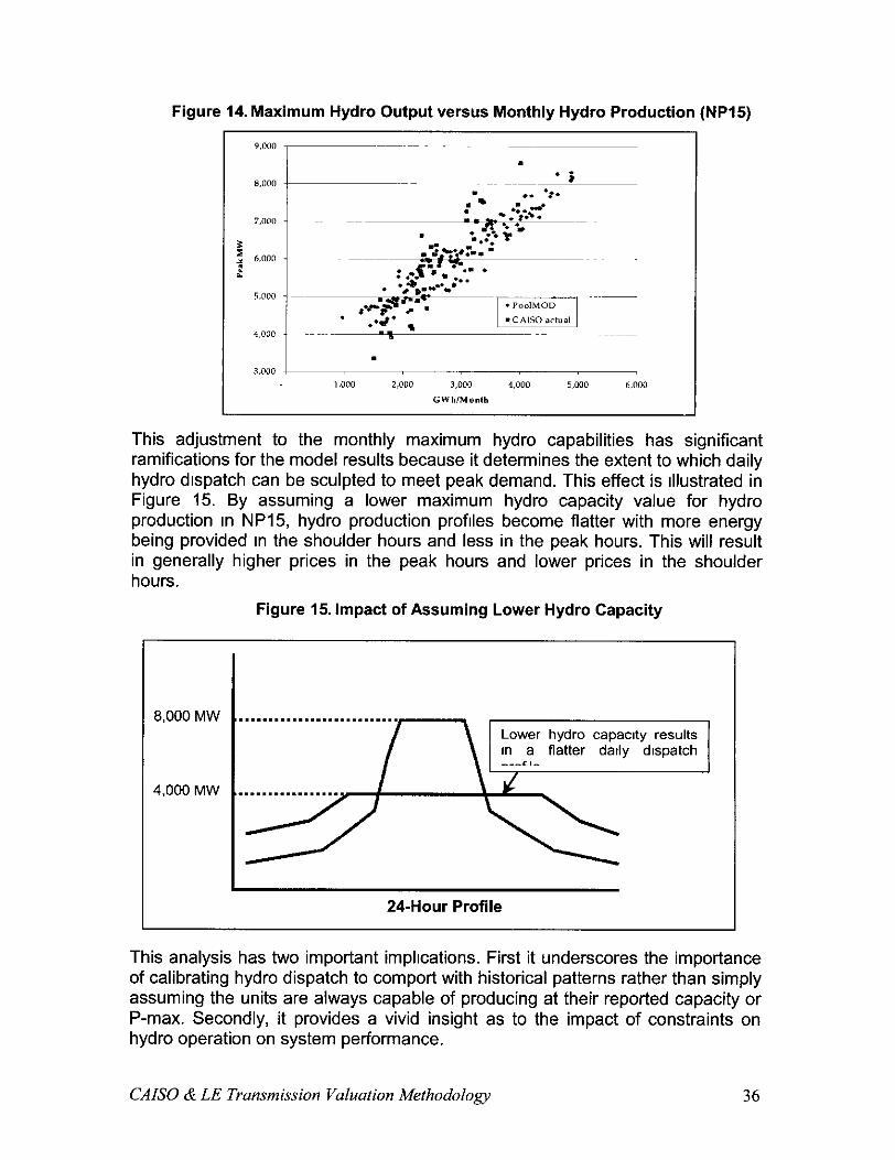
Figure 14. Maximum Hydro Output versus Monthly Hydro Production (NP15)
This adjustment to the monthly maximum hydro capabilities has significant ramifications for the model results because it determines the extent to which daily hydro drspatch can be sculpted to meet peak demand. This effect is rllustrated in Figure 15. By assuming a lower maximum hydro capacity value for hydro production In NP15, hydro production profrles become flatter with more energy being provided in the shoulder hours and less in the peak hours. This will result in generally higher prices in the peak hours and lower prices in the shoulder hours.
Figure 15. Impact of Assuming Lower Hydro Capacity
8,000 MW
4,000 MW
Lower hydro capmty results m a flatter dally dispatch
24-Hour Profile
This analysis has two important implications. First it underscores the importance of calibrating hydro dispatch to comport with historical patterns rather than simply assuming the units are always capable of producing at their reported capacity or P-max. Secondly, it provides a vivid insight as to the impact of constraints on hydro operation on system performance.
CAISO & LE Transmission Valuation Methodology 36
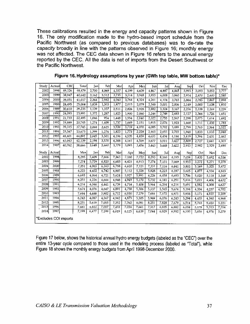
These calibrations resulted in the energy and capacity patterns shown in Figure 16. The only modification made to the hydro-based import schedule from the Pacific Northwest (as compared to previous databases) was to de-rate the capacity broadly in line with the patterns observed in Figure 16; monthly energy was not affected. The CEC data shown in Figure 16 refers to the annual energy reported by the CEC. All the data is net of imports from the Desert Southwest or the Pacific Northwest.
Figure 16. Hydrology assumptions by year (GWh top table, MW bottom table)
Excludes COI imports
Frgure 17 below, shows the historical annual hydro energy budgets (labeled as the “CEC”) over the entire 13-year cycle compared to those used in the modeling process (labeled as ‘Total”), while Figure 18 shows the monthly energy budgets from April 1998-December 2000.
CAISO & LE Transmission Valuation Methodology 31
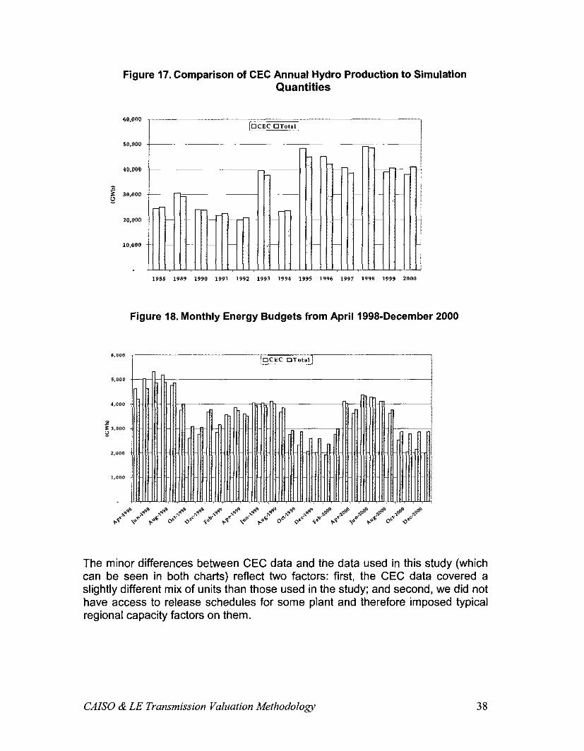
Figure 17. Comparison of CEC Annual Hydro Production to Simulation Quantities
Figure 18. Monthly Energy Budgets from April 1998-December 2000
The minor differences between CEC data and the data used in this study (which can be seen in both charts) reflect two factors: first, the CEC data covered a slightly different mix of units than those used in the study; and second, we did not have access to release schedules for some plant and therefore imposed typical regional capacity factors on them.
CAISO & LE Transmission Valuation Methodoloa 38
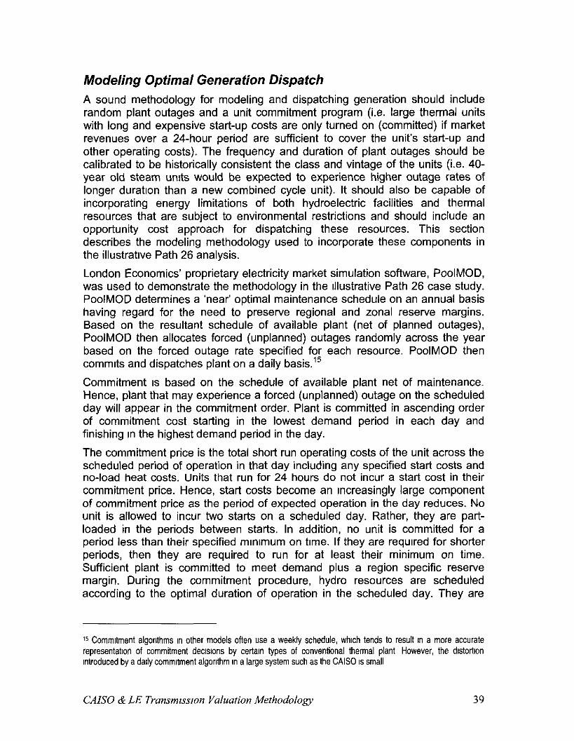
Modeling Optimal Generation Dispatch A sound methodology for modeling and dispatching generation should include random plant outages and a unit commitment program (i.e. large thermal units with long and expensive start-up costs are only turned on (committed) if market revenues over a 24-hour period are sufficient to cover the units start-up and other operating costs). The frequency and duration of plant outages should be calibrated to be historically consistent the class and vintage of the units (i.e. 40- year old steam units would be expected to experience higher outage rates of longer duration than a new combined cycle unit). It should also be capable of incorporating energy limitations of both hydroelectric facilities and thermal resources that are subject to environmental restrictions and should include an opportunity cost approach for dispatching these resources. This section describes the modeling methodology used to incorporate these components in the illustratrve Path 26 analysis.
London Economics’ proprietary electricity market simulation software, PoolMOD, was used to demonstrate the methodology in the Illustrative Path 26 case study. PoolMOD determines a ‘near’ optimal maintenance schedule on an annual basis having regard for the need to preserve regional and zonal reserve margins. Based on the resultant schedule of available plant (net of planned outages), PoolMOD then allocates forced (unplanned) outages randomly across the year based on the forced outage rate specified for each resource. PoolMOD then commrts and dispatches plant on a daily basis.15
Commitment IS based on the schedule of available plant net of maintenance. Hence, plant that may experience a forced (unplanned) outage on the scheduled day will appear in the commitment order. Plant is committed in ascending order of commitment cost starting in the lowest demand period in each day and finishing in the highest demand period in the day.
The commitment price is the total short run operating costs of the unit across the scheduled period of operation in that day including any specified start costs and no-load heat costs. Units that run for 24 hours do not incur a start cost in their commitment price. Hence, start costs become an increasingly large component of commitment price as the period of expected operation in the day reduces. No unit is allowed to incur two starts on a scheduled day. Rather, they are part- loaded in the periods between starts. In addition, no unit is committed for a period less than their specified minimum on time. If they are required for shorter periods, then they are required to run for at least their minimum on time. Sufficient plant is committed to meet demand plus a region specific reserve margin. During the commitment procedure, hydro resources are scheduled according to the optimal duration of operation in the scheduled day. They are
15 Commitment algorithms in other models often use a weekly schedule, which tends to result rn a more accurate representation of commitment declsrons by certarn types of conventional thermal plant However, the drstortron Introduced by a daily commrtment algorithm rn a large system such as the CAlSO IS small
CAISO & LE Transtmsszon Valuation Methodology 39
then given a shadow price just below the commitment price of the resource that would otherwise operate to that same schedule (i.e., the resource they are displacing). Commitment takes account of transmission constraints. A unit is not committed if running that unit at its minimum stable generation would violate a transmission limit. All committed plant in any half-hour period is then deemed to run in that period at its minimum stable generation.
Dispatch is based on the foregoing commitment order. Resources are dispatched to operate above their minimum stable generation based on their incremental heat rates. No other short-run costs are included in the dispatch price. Units on forced outages are not dispatched. No unit is dispatched at a level that would violate a transmission constrarnt. Units are dispatched to meet demand (in contrast to commitment, which utilizes demand plus reserves).
The zonal marginal price is then set equal to the dispatch price of the most expensive dispatched resource in that zone or any electrically interconnected zone not subject to a binding transmissron constraint (i.e. power must be able to flow from the second zone to the first zone - directly or indirectly - in order for a unit in the second zone to set price in the first).
In the current modeling, several simplifying assumptions were made (although PoolMOD does not force these assumptions). Units were assumed to have constant incremental rates across their whole output, and no start costs or no- load heat costs were included.
Finally, both commitment and dispatch prices were adjusted to take account of bid markups from strategic behavror. The mark-ups applied only to Incremental output above a threshold output level.
CAB0 & LE Transmission Valuation Methodology 40
Modeling Demand Price Responsiveness Assumptions about demand side price responsiveness in market simulations can have significant implications on forecasted prices and the ability of suppliers to exercise market power. If demand is assumed to be unable to reduce consumption in the face of higher prices, suppliers will have a greater ability to exercise market power and consequently prices will be generally higher. While the development of price responsive demand is a high priority for most restructured electricity markets, these efforts have to date yielded only nominal results. Given the importance of this component, a transmission valuation study should examine the sensitivity of the benefit results to different assumptions about price-responsive demand.
There are two approaches to incorporating price responsive demand Into a transmission valuation model: the demand curve can be modeled as a function of price (i.e. a price responsive demand curve is assumed rather than a vertical inelastic demand curve) or price responsive demand could be incorporated into the supply function as curtailable demand (i.e. demand that is willing to curtail once prices reach a certain level(s)). These two approaches are very different in that under the first approach, load reduces consumption to “avoid” having to pay higher prices but under the second approach load is “paid” to reduce consumption. From a policy standpoint, some have questioned the efficiency of the latter approach because it requires verification that curtailments actually took place. However, from a modeling standpoint, both approaches produce the same effect (i.e. consumption goes down when prices go up). In addition, the latter approach is advantageous because it simplifies the benefit calculations for determining consumer surplus. This issue is discussed in greater detail in Section VI - Measuring Net-Benefits.
In the illustrative Path 26 analysis, demand side responsiveness is modeled as dispatchable demand. Hence, these resources are committed and dispatched in the same manner as, for example, a peaking gas turbine. It is assumed that NP15 contains 256MW of curtailable demand in six blocks, ranging in price from $250/MWh to $650/MWh. SP15 contains similar resources, but the block size is 174MW (giving a total of 1,043MW). ZP26 contains 4 blocks of 1 IMW of curtailable demand priced from $250/MWh to $650/MWh. The price range and level of curtailable demand used in this analysis is roughly commensurate with the prices and level of participation observed in the day-ahead load curtailment programs implemented by the California UDCs in Summer 2000. Under these programs, the UDCs paid customers to reduce consumption when prices in the day-ahead PX Market exceeded $250/MWh.
Under this approach, sensitivity analysis could be performed for this modeling component by assuming different quantity and price levels of curtailable demand in each zone. However, time did not permit for such analysis under the illustrative Path 26 study.
CAISO & LE Transmission Valuation Methodology 41
Modeling Long-term New Generation En try There are many uncertarn elements to consider when conducting a cost benefit analysis for a transmission investment project, but by far, the most challenging uncertainty revolves around the interdependence of generation and transmission assets. The benefits flowing from a transmission investment depend on uncertain future demand for transmission services, and this demand in turn depends on the expected pattern of new generation investment. To determine the optimal transmission investment schedule it is therefore necessary to take account of the incentives to invest in generation. This problem is further complicated by the fact that the relationshrp between the demand for transmission and the demand for generation services varies over trme and space. In some cases generation and transmission are substitutes for each other: a generation asset produces power at a specific location, while transmrssion delivers power to a specific location. However, under other conditions, generation and transmission projects are also complementary investments: a transmission line expansion may improve the profitability of a generator that is exporting power, as it increases the volume of power that the exporting generator can sell and cause to be delivered.
Additional power requirements in any particular region can be satisfied by investment in generation in that region, or by grid augmentation investment that allows a higher volume of imported power to be delivered. If a single entity with appropriate incentives were responsible for both generation and transmission investment then, faced with additional demand, it would seek the least cost form of supply; trading off the costs and benefits of transmission and generation investmentI However, with restructuring, the decision-making capabilities of the transmission planner are no longer integrated with that of generation. While publrcly accountable for the efficient and reliable delivery of power, the CAISO only has control over one of the two means by which capital allocations can advance this goal. Thus, in order to optimize transmission investment, the CAISO needs to be able to anticipate potential investment in generation in response to transmission investment and incorporate the interdependence of transmission and generation into the valuation process for transmission.
A methodology for incorporating new generation investment under different transmission expansion options IS described below.
Entry Decision For each transmission upgrade option, a pattern of long-term new generation entry is derived under the assumptions that, (i) new entry are independent and non-strategic; (ii) new entry will be just sufficient to maintain prices at the appropriate remunerative levels. These appropriate remunerative levels are defined as a benchmark annual revenue requirement, also called “entry trigger
‘6 Demand side management IS obviously also an optlon that needs to be consldered, but this does not affect the fundamentals of the argument.
CAB0 & LE Transmission Valuation Methodology 42
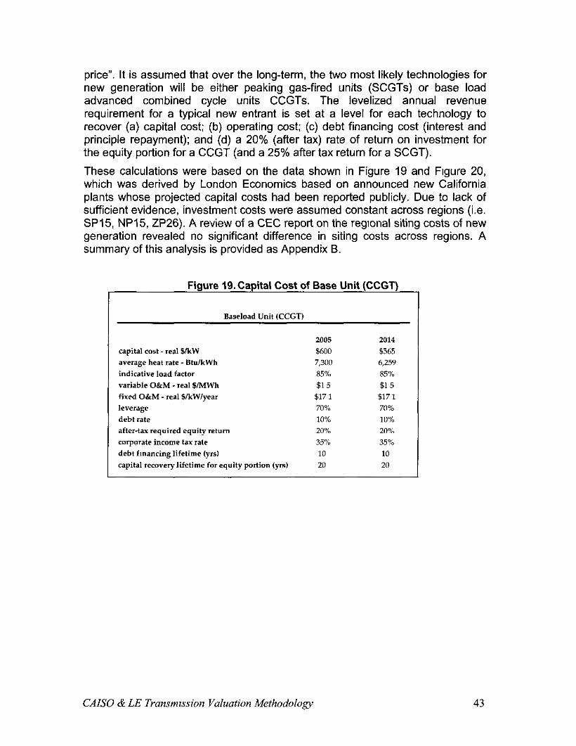
price”. It is assumed that over the long-term, the two most likely technologies for new generation will be either peaking gas-fired units (SCGTs) or base load advanced combined cycle units CCGTs. The levelized annual revenue requirement for a typical new entrant is set at a level for each technology to recover (a) capital cost: (b) operating cost; (c) debt financing cost (interest and principle repayment); and (d) a 20% (after tax) rate of return on investment for the equity portion for a CCGT (and a 25% after tax return for a SCGT).
These calculations were based on the data shown in Figure 19 and Frgure 20, which was derived by London Economics based on announced new California plants whose projected capital costs had been reported publicly. Due to lack of sufficient evidence, investment costs were assumed constant across regions (i.e. SPI 5, NPI 5, ZP26). A review of a CEC report on the regronal siting costs of new generation revealed no significant difference in siting costs across regions. A summary of this analysis is provided as Appendix B.
Figure 19. Capital Cost of Base Unit (CCGT)
Baseload Unit (CCGT)
capital cost - real $kW average heat rate - BtukWh indicative load factor variable O&M-real $IMWh fixed O&M-real $kW/year leverage debt rate after-tax required equity return corporate income tax rate debt fmancing lifetime (yrs) capital recovery lifetime for equity portion (yrs)
$600 7,300 85% 515
$171 70% 10% 20% 35% 10 20
2014 5565 6,259 85% 51 5
$17 1 70% 10% 20% 35% 10 20
1 I
CAISO d; LE Transrmssion Valuation Methodology 43

Figure 20. Capital Cost of a Peaking Unit (SCGT)
Peaking Unit (SCGT)
capital cost-real $/kW average heat rate - BhAWh indicative load factor variable O&M-real $iMWh fixed O&M - real $IkW/year leverage debt rate after-tax required equity rehlm
2005 2014 $350 $329
11,000 9,631 10% 10% 519 519 $8.0 58 0 30% 30% 10% 10% 25% 25%
corporate income tax rate financing lifetime (yrs) capital recovery lifetime for equity portion (yrs)
35% 35% 10 10 10 10 I
Given the capital costs cited above, entry trigger prices are calculated for each year and each zone, based on the capacity factors derived by PoolMOD for each new unit type (SCGT, CCGT). In addition PoolMOD calculates the average unit revenue (AUR) for each new unit type. The addition of new units is then based on a comparison of AUR and trigger prices until the model converges to a point where it is no longer profitable for new entry. Long-term new generation entry was derived separately for each transmission option to reflect the potential substitutability of new generation for new transmission Entry decrsions were based on the predicted market clearing prices (i.e. prices that reflect the impact of strategic bidding behavior) rather than competitive prices.
Entry decisions were based on a probability-weighted average of prices under low, medium, and high demand scenarios, assuming normal gas prices, to reflect the fact that entry decisions are based on expected profits under a variety of system condrtions. ideally, one would want to consider expected profits under alternative hydro and gas price scenarios as well. However, because new generation entry is added incrementally in an iterative process, it was not practically feasible to consider more scenarios than the three demand scenarios described above.
CAB0 & LE Transmissron Valuation Methodology 44
Modeling Market Power In a restructured electricity market, transmission expansions can provide significant consumer benefits by improving market competitiveness. A transmission expansion can increase market competitiveness by increasing both the number of suppliers available to serve load and the total available supply. The number of suppliers is of particular importance because as more suppliers are able to compete for demand, the market becomes less concentrated and more competitive. Of course, a transmission expansion is just one of several structural options for improving market competitiveness. The addition of new generation capacity, increased levels of forward energy contracting, or the development of price responsive demand can also significantly reduce the ability of suppliers to exercise market power in the spot market. However, a transmission expansion has the additional benefit of improving the competitiveness of not just the spot market but also the longer-term forward energy market. Thus occurs because the transmission expansion creates greater access to a broader regional market and thereby increases the number of sellers that could offer long-term energy contracts. A comprehensive transmission expansion study should explore the market power mitigation benefits of a transmissron upgrade under a variety of plausible new generation entry, forward contracting levels, and price responsive demand scenarios.
Some have argued that it is inappropriate to include the market power mitigatron benefits of a transmission expansion in an assessment of the benefits of a transmission expansion and that market power IS more appropriately addressed through effective regulation. The CAISO believes that trusting that regulators will have the political will and/or ability to effectively enforce regulations to eliminate market power is a high-risk strategy that could have enormous consequence to consumers if regulators are unable or unwilling to control market power. The California experience In year 2000 is a case in point. We also believe that in the long run, the most effective way to mitigate market power is to correct the structural deficiencies that enable suppliers to exercise market power (e.g lack of supply, lack of forward contracting, and lack of price responsive demand).
This section examines two approaches to modeling strategic bidding behavior (e.g. the exercise of market power) In transmission valuation studies. The first approach involves developing a game theoretic model of strategic bidding. The second approach involves capturing strategic bidding through estrmated historical relationships between certain market variables and a variable that captures a measure of market power such as the difference between estimated competitive prices or bids and actual prices and bids (i.e. price-cost markups and bid-cost markups, respectively). Each modeling approach has its advantages and disadvantages.
The advantage of the game theoretic approach is that because it is derived independent of observed historical behavior, it can simulate market power under a variety of future market conditions without the potential bras of having been based on observed historical behavior. This could be particularly important if the
CAISO & LE Transmisston Valuation Methodology 45

market conditions assumed in the model study period are very different than past historical conditions. For example, if a study assumed a much higher level of forward energy contracting or price responsive demand than existed historically, a game theoretic model that explicitly incorporates these elements in determining strategic bidding may be able to better simulate market power than an empirical approach that is based on a period where there was very little forward contracting. However, the game theoretic model’s independence from observed historical relationships between market power and specific market conditions raises a significant risk in that if the model is not tested and calibrated to replicate historical bidding practices, there is no guarantee that it will be able to accurately predict strategic bidding in the future. Moreover, it may simply not be possible to calibrate a game theoretic model to match actual market outcomes given that there are a limited number of instruments one can incorporate and adjust in such a model. Another risk in simulation-based game theoretic models is that the converged solution may not be truly converged or represent a true equilibrium. This can happen if the strategy space is too narrowly defined or if the limit on the maximum number of iterations is set too low. It may also happen if the model is simply too complicated to converge to a solution. In order for a game theoretic model to solve in a tractable and timely manner, the model must be fairly simplrstic in terms of network representation and the types of bidding strategies. Such simplifications may make the model too abstract to reasonably capture market power.
The advantage of modeling market power through an empirical approach where estimates of historical relationships between market power (as expressed through bid-cost or price-cost markups) and certain market variables (such as load levels and supply margins) are applied prospectively in the transmrssion study IS that the approach has a strong historical basis. Another advantage IS that this approach could be applied to a more detailed transmission network representation provided the model can produce the required explanatory variables (i.e. the variables contained In the regression equation(s)) at a more granular level. A potential disadvantage of this approach is that because it is based on estimated historical relationships, its predictive capability may be limited if applied under very different market conditions.
Given that both approaches have complementary strengths and weaknesses and that work in this area is relatively new, we have developed versions of both approaches and applied them in the illustrative case study of Path 26. Each of these approaches is discussed in greater detail below.
Game Theoretic Models Game theoretic models typically consist of several strategic suppliers with each player seeking to maximize its expected profits by changing its bidding strategy in response to the bidding strategies of all other players. An equilibrium is attained when no player can increase its expected profits given the bidding strategies of all other players. In very simplistic game theoretic models, an equilibrium can be solved for mathematically. In more complicated models, an
CAISO & LE Transmission Valuatzon Methodology 46

equilibrium cannot be solved directly but must instead be derived through an iterative process where each player’s bid is adjusted based on the observed bidding behavior of all other players in the previous iteration. The model converges when no player wants to change its bid strategy, given the bid strategies of all other players in the previous iteration. A meaningful model of strategic bidding in a transmission study must recognize the major constraints in the transmission network and the location of each player’s supply within the network. These requirements generally make the model too complex for determining a solutron mathematically and thus an iterative convergence approach is necessary.
An iterative model of strategic brdding, “ConjectureMod”, was developed by London Economics and applied in the illustratrve case study of Path 26. The term “ConjectureMod” (CM) is derived from the central tenet of the model, namely that strategic behavior is simulated through an iterative process in which participants conjecture that their competitor bids are some function of their profit maximizing bids in previous iterations. The model then produces details of each iteration, which include bid markups on players’ marginal costs, portfolio average unit revenue and regional prices.
The starting point of this iterative procedure is that each bidder i predicts that each other bidder j is bidding its marginal cost at output level q,, i.e., P,(q,) = MC,(q,). Then, for each demand level D bidder i chooses its offered bid pair (P,(q,;D), q,) according to an assumed supply function form (see discussion in below) to maximize its net profit in view of its residual demand function given D and its prediction of other bidders’ supplies. For the iterative procedure thereafter, each firm conjectures that each players bid is their profit maximizing bid from the previous iteration.
CAISO & LE Transmission Valuatron Methodology 47

The discontinuous nature of the supply curve and the solution methodology underlying production-cost simulation and traditional transport models does not allow specification of a continuous strategy space. Rather, each player’s supply function is assumed to take the following form:
4&J = W,zh,d - 4. + k b,z(q,z) s fOO0 where MC,Z(q,d is the marginal cost of generator j in zone k at output q,z, k is a constant which could be considered similar to the intercept used in linear SFE models and /.r is a discrete strategy choice E (1, 1.1, 1.3, 1.5, 2, 3, 4, 5, 10, 15, 20, 25, 30, 3540). Furthermore:
l k was indexed against prevarling gas prices to ensure that the mix of strategic plant is not affected by the gas price assumption in the model; and
l units that bid strategically are assumed to bid marginal costs on their capacity up to elbow point 1 (typically the first third of their total capacity), and strategically only on capacity in excess of this figure.17
Convergence rules were set such that the model was deemed to have converged if the profits of each and every player do not diverge across the last two iterations by more than I%, or when 50 iterations are complete.
The profit for each player is based on the relevant zonal prices having regard to any transmission constraints, and also takes into account the revenue impacts of any long-term contracts that may apply to that player.
ConjectureMOD is closely integrated with PoolMOD. It estimates markups for all resources based on the same schedule of resources used by the PoolMOD commitment algorithm, and uses the same algorithm to determine transmission constratnts.
I7 The assumption closely follows observed behawor in markets such as E&W and SE Australia
CAISO & LE Transmission Valuation Methodology 48

Empirical Approach An empincal approach to modeling market power was developed in this study through estimating the historical relationships between certain market variables and observed price-cost markups. The basic approach involved developing historical measures of price-cost markups as a function of system conditions and utilizing those estimated relationshlps to model market power prospectively under the various system conditions assumed in a transmission valuation study.
The approach entails four major steps.
1. Complete a price-cost markup regression analysis using hrstorical data (Nov 99 - Ott 00) where the hourly price-cost markup in each zone (j) is regressed against a residual supply index (RSI,,,) - a measure of the extent to which the largest supplier is “pivotal” in the market, Uncommitted Capacity of the largest single supplier in the zone (TUC,,,), the total zonal load (LD,,,), a dummy variable for whether it is a summer month (SP,,,), and a dummy variable for whether the zone is NP15 or SP15 (NS,,,).
2. Under the various supply and demand scenarios considered in the prospective transmission valuatron study, determine for each hour (i) and zone (j):
% Residual Supply Index (RSI,,,)
k Identity of Largest Single Supplier (LSS,,,)
> Total Uncommitted Capacity of LSS,,, (TUC,,,)
> Zonal Load (LD,,,)
3. Apply the regresslon equation(s) in Step 1 to the values derived in Step 2 to estimate the price-cost markups in each zone and apply the estimated price-cost markups to the competitive based MCPs in each zone to compute market-clearing prices under the various supply and demand scenarios.
4. Calculate new generatron investment for the base case scenarios through iterations between competitive PoolMOD and the application of the estimated price-cost markups.
Each of these steps is described in greater detail below.
CAISO & LE Transmission Valuation Methodology 49
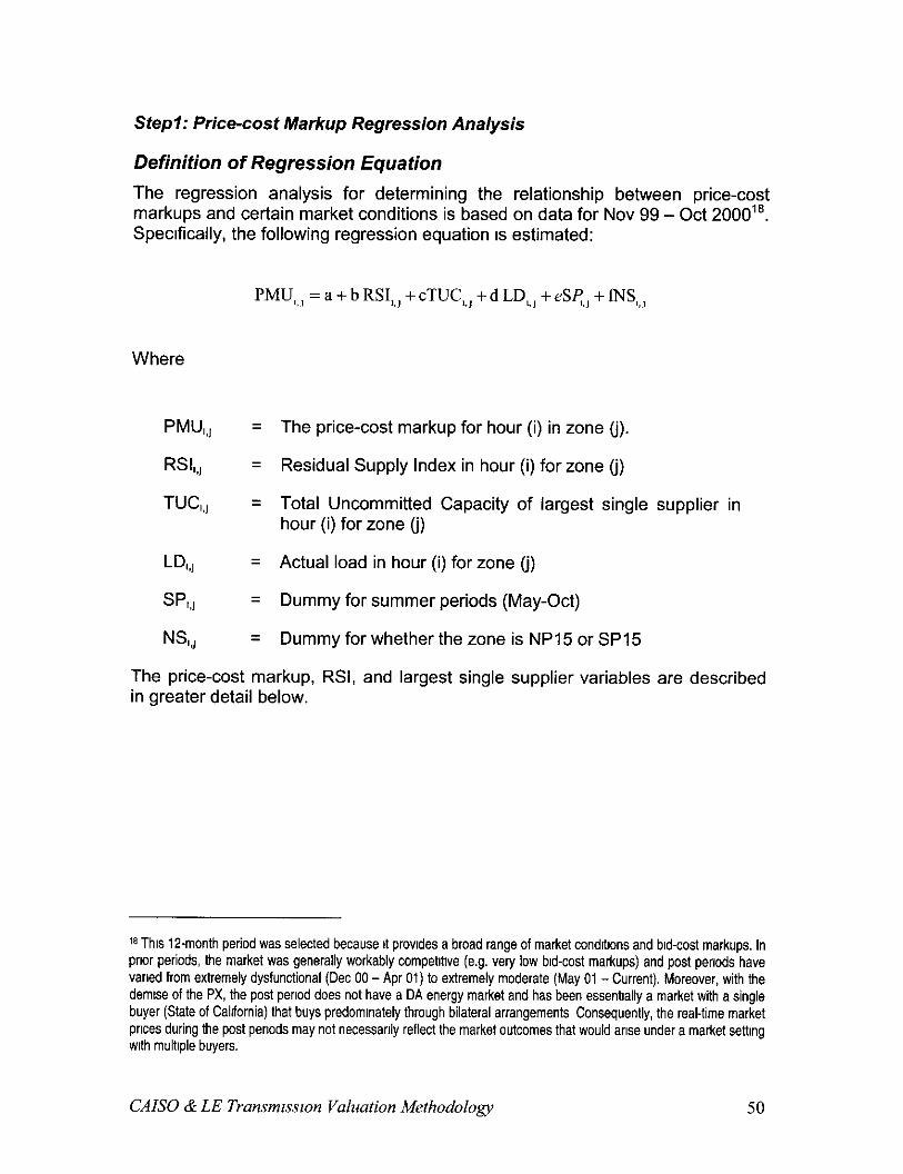
Stepl: Price-cost Markup Regression Analysis
Definition of Regression Equation The regression analysis for determining the relationship between price-cost markups and certain market conditions is based on data for Nov 99 - Ott 2000”. Specrfically, the following regression equation IS estimated:
PMU,,, = a + b RN,, + cTUC,, + d LD,,, + es<,, + fNS,,
Where
PW,, = The price-cost markup for hour (i) in zone (j).
W,, = Residual Supply Index in hour (i) for zone (j)
TW,, = Total Uncommitted Capacity of largest single supplier in hour (i) for zone (j)
LQ, = Actual load in hour (i) for zone (j)
SPI,, = Dummy for summer periods (May-Ott)
NS, = Dummy for whether the zone is NP15 or SP15
The price-cost markup, RSI, and largest single supplier variables are described in greater detail below.
I8 This 1%month period was selected because it prowdes a broad range of market condltlons and bid-cost markups. In prior periods, the market was generally workably competltlve (e.g. very low bid-cost markups) and post periods have varied from extremely dysfunctional (Dee 00 - Apr 01) to extremely moderate (May 01 -Current). Moreover, with the demise of the PX, the post period does not have a DA energy market and has been essentially a market with a single buyer (State of Cakfornia) that buys predommately through bilateral arrangements Consequently, the real-time market prices during the post periods may not necessarily reflect the market outcomes that would arise under a market settmg with multlple buyers.
CAB0 & LE Transmlssron Valuation Methodology 50
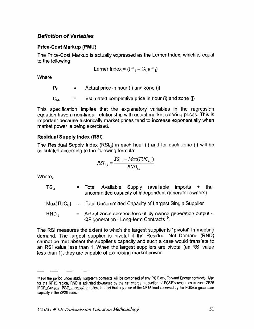
Definition of Variables
Price-Cost Markup (PMU)
The Price-Cost Markup is actually expressed as the Lerner Index, which is equal to the following:
Lerner Index = ((P,,, - C,,,)/P,,,)
Where
PI,, = Actual price in hour (i) and zone (j)
cu = Estimated competitive price in hour (i) and zone (j)
This specification implies that the explanatory variables in the regression equation have a non-linear relationship with actual market clearing prices. This is important because historically market prices tend to increase exponentially when market power IS being exercised.
Residual Supply Index (RSI)
The Residual Supply Index (RSI,,,) in each hour (i) and for each zone (j) will be calculated according to the following formula:
Where,
RSI,,, = Ts,,, - M4TuC,,, 1
WD,,,
TS,, = Total Available Supply (available imports + the uncommitted capacity of independent generator owners)
Max(TUC,,,) = Total Uncommitted Capacity of Largest Single Supplier
RN& = Actual zonal demand less utility owned generation output - QF generation - Long-term Contracts’g.
The RSI measures the extent to which the largest supplier is “pivotal” in meetrng demand. The largest supplier is pivotal if the Resrdual Net Demand (RND) cannot be met absent the supplier’s capacity and such a case would translate to an RSI value less than 1. When the largest suppliers are pivotal (an RSI value less than ‘I), they are capable of exercising market power.
(9 For the period under study, long-term contracts will be comprrsed of any PX Block Forward Energy contracts Also for the NP15 region, RND IS adjusted downward by the net energy production of PG&E’s resources in zone ZP26 [PGEGenzPx - PGE-Loadzps] to reflect the fact that a portton of the NP15 load IS served by the PG&E’s generatlon capacity in the ZP26 zone.
CAISO & LE Transmission Valuation Methodology 51
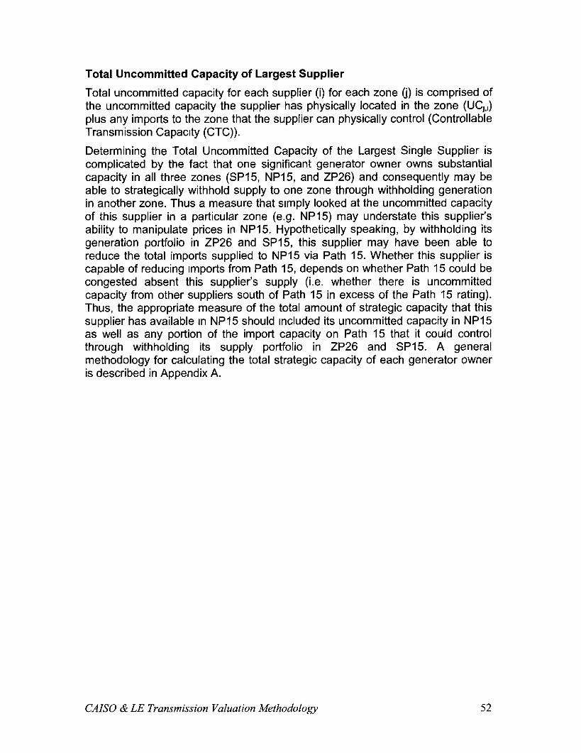
Total Uncommitted Capacity of Largest Supplier
Total uncommitted capacity for each supplier (i) for each zone (i) is comprised of the uncommitted capacity the supplier has physically located in the zone (UC,,,) plus any imports to the zone that the supplier can physically control (Controllable Transmission Capacrty (CTC)).
Determining the Total Uncommitted Capacity of the Largest Single Supplier is complicated by the fact that one significant generator owner owns substantial capacity in all three zones (SP15, NP15, and ZP26) and consequently may be able to strategically withhold supply to one zone through withholding generation in another zone. Thus a measure that srmply looked at the uncommitted capacity of this supplier in a particular zone (e.g. NP15) may understate this supplier’s ability to manipulate prices in NP15. Hypothetically speaking, by withholding its generation portfolio in ZP26 and SP15, this supplier may have been able to reduce the total imports supplied to NP15 via Path 15. Whether this supplier is capable of reducing rmports from Path 15, depends on whether Path 15 could be congested absent this supplier’s supply (i.e. whether there is uncommitted capacity from other suppliers south of Path 15 in excess of the Path 15 rating). Thus, the appropriate measure of the total amount of strategic capacity that this supplier has available In NP15 should Included its uncommitted capacity in NP15 as well as any portion of the import capacity on Path 15 that it could control through withholding its supply portfolio in ZP26 and SP15. A general methodology for calculating the total strategic capacity of each generator owner is described in Appendix A.
CAISO & LE Transmission Valuation Methodology 52
Total Available Supply
Capacity on Major Inter-Ties The determination of total supply for each zone must include an assessment of how much energy is actual available at the inter-ties. The critical term here is “available” because from a market power standpoint, the ability of a market to compete away any attempt to exercise market power stems from the amount of supply capacity available as opposed to what was actually generated. When there is an abundance of capacity in the market, suppliers will bid aggressively (i.e. close to their actual marginal cost) since they know if they bid too high, they will not be selected.
Modeling the amount of “available supply” on the Pacific Northwest inter-ties is complicated by the fact that actual scheduled flows In any hour may not be indicative of the total available supply Moreover, using the total import transmission capability may overstate the actual available supply, particularly during dry periods. An alternative is to base the available import capability on schedules and submitted RT bids. However, this approach would tend to understate the available supply if participants tend not to offer into the real-time market in hours when prices are expected to be relatively low. Given these difficulties, the followlng approach was used for determining the available supply on the major Northwest path into California (COl).20
Available Transmission Capacity on CO/ (Import Direction):
ATC-COI, = Mm[Max[O, Maximum hourly flow for operating day)], Grp-lmf]
Under this formulation, the assumed available supply in each hour is set to the lower of the maximum hourly scheduled net-imports for that operating day and the transmission import limit for that hour. The transmission import limit (Grp-lmt) is the total transmission capability less any unused ETC reservations”. This approach assumes that the maximum hourly schedule for each operating day represents the maximum supply available for each hour of that day. While this is not a perfect measure, it strikes a reasonable compromise between assuming the hourly scheduled flow as the total available capacity, which would tend to understate the total available supply, and assuming the hourly transmission limit (Grp-lmt,,,), which would tend to overstate the total available supply.
20 A similar approach could be adopted for the Pacific Northwest DC line Into Southern Callfomra. However, this path was not modeled in the market slmulatlon software and therefore was not Included in the regression. Ideally, the Paclflc Northwest DC lkne (NOB) would be modeled in both the regresslo” analyw and in the prospective transmission valuation methodology.
21 Capacity for Exlstlng Transmlsslon Contracts (ETCs) are often reserved In the day-ahead market but never utilized Since this unscheduled ETC capacity IS not avaIlable to the market, It IS subtracted from the total transmwon capabIlIty
CAB0 & LE Transmission Valuation Methodology 53
Measuring the available supply for each hour on the southwest inter-ties is also challenging. As with the Pacific Northwest inter-ties, using the hourly net-import schedules on the Desert Southwest inter-ties as the measure will tend to underestimate the total available supply. Using the total transmission limit (Grp-lmt,) may be appropriate during off-peak periods but could significantly over-state available supply during summer peak periods when scheduled imports from the southwest are fairly low. As was previously discussed, during the summer peak periods, the available supply from the Desert Southwest tends to be inversely related to load levels in California. This occurs because California’s summer peak loads are highly correlated with the Desert Southwest peak loads. Thus during simultaneous peaks, there is less supply available from the Desert Southwest for import into California. To capture this phenomenon, the following approach was used to determine the available supply on southwest paths to Calrfornia:
Available Transmission Capacity on the major Southwest Interfaces (Palo Verde, Mead, Eldorado, Silver Peak):
ATCSW, = the lowest of the following:
1. Max[O, maximum hourly flow for operating day)],
2. Grpplmt,, and
3. Maximum import capability for the load category (L) (this 3’cl term only applies in Jun-Sep in hours where hourly CAISO loads exceed 38,000 MW).
The maximum Import capabrlrty for load category L, is computed as:
MaafO, 9 Act&Flow, ] x4
Where the load category is defined in 1 GWh increments from 38- 46 GWh and “x” represents the different inter-ties between southwest and CAlSO control area.
For instance, maximum import capacity for the load category between 38,000 MW and 39,000 MW would be the largest import quantity recorded where the load is between 38,000 MW and 39,OOOMW in the summer months. This third term is included to reflect the fact that during high load periods, the amount of supply available on the SW branch groups typically declines because CAISO summer peak loads are highly correlated with the Desert Southwest peak loads leaving less supply available for import into California.
CAISO & LE Transmission Valuation Methodology 54
Another important import supply for the CAlSO control area are the inter-ties connecting to the Los Angeles Department of Water and Power (LADWP). Since LADWP’s loads are also highly correlated with loads In the CAlSO control area, the same approach used to determine available supply for the southwest inter- ties was used for the inter-ties with LADWP.
Available Transmission Capacity for the infer-ties connecting to I-ADWP @y/mar, Mccullgh, Inyo, andVktv/):
ATC-LA, = Same approach as ATC-SW,
Capacity on internal paths:
Since price-cost markups are estimated on a zonal basis, it is also necessary to make certain assumptions about the amount of available supply on the two major internal paths (Path 15 and Path 26) that define the three major internal zones In the CAISO control area (NP15, ZP26, and SP15). The available supply on the internal paths was determined by taking the lower of the total uncommitted supply in exporting zones and the path limit (Grpplmt). For example if in a particular hour, the total supply In NP15 that could be exported to ZP26 (T&z) is 700 MWh and the Path 15 lrmit for that hour in the north-south direction is 806 MW (Grp-1mtn.z) then the available supply on Path 15 north to south (AT&z) would be set equal to 700 MW. This value would then be combrned with the total uncommitted supply in ZP26 to determine the maximum amount that could be exported to SP15.
Path 15 north to south:
AT&z = Min [T&z, Grp-1mtN.z of Path 151
Where,
TSN-z = ATC-COI+ XlJ’&~s + Other Generation**
Path 26 north to south:
AT& = Min [T&s, Grp-lmtzs of Path 261
Where,
T&s = AT&z + XUCzp26
22 Other generation Includes generatlon from faclktles other than the fwe new generatton owners (Dynegy, Duke, AESNVlllrams, Mlrant, and Rekant), UDC owned faclllties, and qualifying facllltles (QFs) Calpme was not Included because their gas-flred capacity was not on-lme dung the study perlod used In th6 regressEon analysis.
CAISO & LE Transmission Valuation Methodology 55
Path 26 south to north:
ATCs.z = Min [T&z, Grpplmts.zof Path 261
T&-z = ATCsw + AT& + ZlJCspz6 + Other Generation
Path 15 south to north:
AT&a
Where
= Min [T&N, Grp-1mtz.N of Path 151
-Z-N = AT&z + [PGE-GenzpzB - PGE-LoadzP26]+ CUCzp2s
The total supply available from ZP26 to NP15 (T&J) includes the available transmission capabikty from SP15 to ZP26 (ATCz.r.J, the net PG&E generation (i.e. Diablo generation less PG&E load in ZP26), and the total uncommitted capacity of all other suppliers in ZP26 (BJCzp26)
Total available supply in NPIS:
Total Available Supply in NP15 is defined as follows:
TSw,,,z = f %wm,,~ + (ATC,., , - [PGE_GenZP26 - PGE-LoadZP261) + AT&,,, rn=I
+ Metered Generation From Other Generators Other than NGOs,UDC, and QFs
= the sum of the uncommitted capaciv3 of the two major independent generator owners in NP15 (Duke and Mirant).
The Capacity of Path 15 from south to north is further reduced by [PGE-Genzppc - PGE-LoadZP26] to reflect the fact that most of energy generated by the PG&E owned Diablo facility in ZP26 zone serves load in NP15. Diablo’s net of load generatron in ZP26 is also subtracted from the NP15 Residual Net Demand (RNDNP~s) in the RSI calculation (i.e. counted as utility owned generation output).
23 Uncommrtted capackty for each generator owner IS equal to the total awlable capacity less any capacity commltted under long-term contracts
CAISO & LE Transmission Valuation Methodology 56

Total Supply in SPl5 The Total Supply for SP15 WIII be calculated as follows:
Where,
the sum of the uncommitted capacrty of the three major Independent generator owners in SP15 (Williams,
Summary of Estimation Methodology In summary, the computation of the variables described above will result in a data set havmg 4 variables for each hour (i) and zone (j) (PMU,,,, RSI,,,, UC,,,, and LD,,,) for all 8,765 hours from Nov 99 - Ott 00. These data will be used to estimate the regression equation based on the following relation:
PMU,,, = a + b RSI,,, + cTUC,,, + d LD,, + es<,, + fNS,,
Where
PM&
RSI,,,
TUC,,,
= Price-Cost Markup for hour (i) in zone (j).
= Residual Supply Index in hour (i) for zone (j)
= Total Uncommitted Capacity of largest single supplier in hour (i) for zone (j)
4 = Actual load in hour (i) for zone (j)
spu = Dummy for summer periods (May-Ott)
W,, = Dummy for whether the zone is NP15 or SP15
CAISO & LE Transmwion Valuation Methodology 57
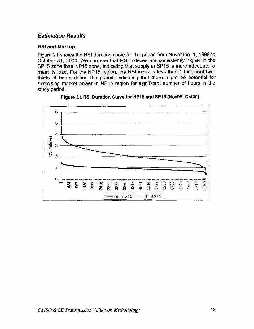
Estimation Results
RSI and Markup
Figure 21 shows the RSI duration curve for the period from November 1, 1999 to October 31, 2000. We can see that RSI indexes are consistently higher in the SP15 zone than NP15 zone, indicating that supply in SP15 is more adequate to meet its load. For the NP15 region, the RSI index is less than 1 for about two- thirds of hours during the period, indicating that there might be potential for exercising market power in NP15 region for significant number of hours in the study period.
Figure 21. RSI Duration Curve for NP15 and SP15 (Nov99-OctOO)
6 ------
5
CAB0 & LE Transmission Valuatron Methodology 58
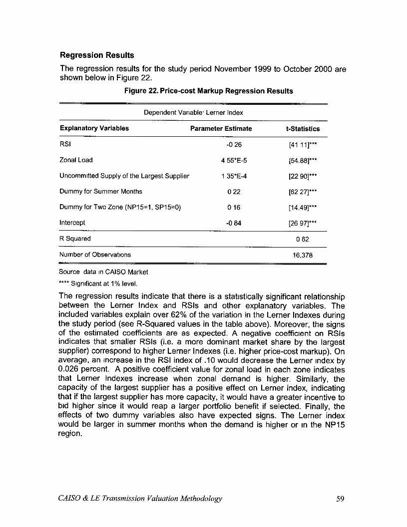
Regression Results
The regression results for the study period November 1999 to October 2000 are shown below in Figure 22.
Figure 22. Price-cost Markup Regression Results
Dependent Vanable Lemer Index
Explanatory Variables Parameter Estimate t-Statistics
RSI -0 26 [41 II]*”
Zonal Load 4 55*E-5 [54.88]**
Uncommitted Supply of the Largest Supplier 1 35*E-4 [22 901***
Dummy for Summer Months 022 [62 271"'
Dummy for Two Zone (NP15=1, SP15=0) 016 p4.491”
Intercept -0 84 [26 97]**’
R Squared 062
Number of Observations
Source data m CAISO Market
16,378
**** Slgnlficant at 1% level.
The regression results indicate that there is a statistically significant relationship between the Lerner index and RSls and other explanatory variables. The included variables explain over 62% of the variation in the Lerner Indexes during the study period (see R-Squared values in the table above). Moreover, the signs of the estimated coefficients are as expected. A negative coefficient on RSls indicates that smaller RSls (i.e. a more dominant market share by the largest supplier) correspond to higher Lerner Indexes (i.e. higher price-cost markup). On average, an Increase in the RSI index of .I0 would decrease the Lerner Index by 0.026 percent. A positive coefficient value for zonal load in each zone indicates that Lerner Indexes increase when zonal demand is higher. Similarly, the capacity of the largest supplier has a positive effect on Lerner index, indicating that if the largest supplier has more capacity, it would have a greater incentive to bid higher since it would reap a larger portfolio benefit if selected. Finally, the effects of two dummy variables also have expected signs. The Lerner index would be larger in summer months when the demand is higher or in the NP15 region.
CAISO & LE Transmission Valuation Methodology 59
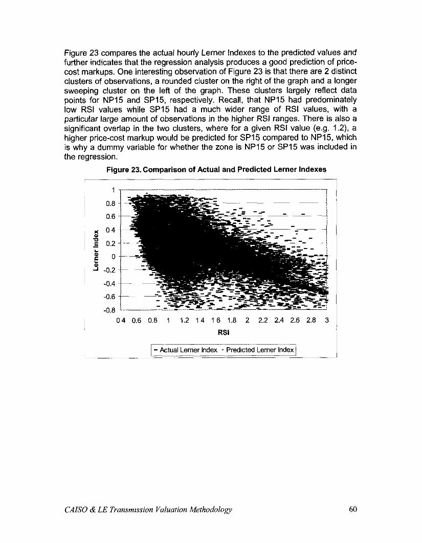
Figure 23 compares the actual hourly Lemer Indexes to the predicted values and further indicates that the regression analysis produces a good prediction of price- cost markups. One interesting observation of Figure 23 is that there are 2 distinct clusters of observations, a rounded cluster on the right of the graph and a longer sweeping cluster on the left of the graph. These clusters largely reflect data points for NP15 and SP15, respectively. Recall, that NP15 had predominately low RSI values while SP15 had a much wider range of RSI values, with a particular large amount of observations in the higher RSI ranges. There is also a significant overlap in the two clusters, where for a given RSI value (e.g. 1.2) a higher price-cost markup would be predicted for SP15 compared to NP15, which is why a dummy variable for whether the zone is NP15 or SP15 was included in the regression.
Figure 23. Comparison of Actual and Predicted Lerner Indexes
z 04
E 0.2
k : 0
i J -0.2
-0.4
-0.6
-0.8
r c
I 04 0.6 0.8 1 1.2 14 16 1.8 2 2.2 2.4 2.6 2.8 3
RSI
- Actual Lerner index - Predicted Lerner Index
CAB0 & LE Transmssion Valuation Methodology 60
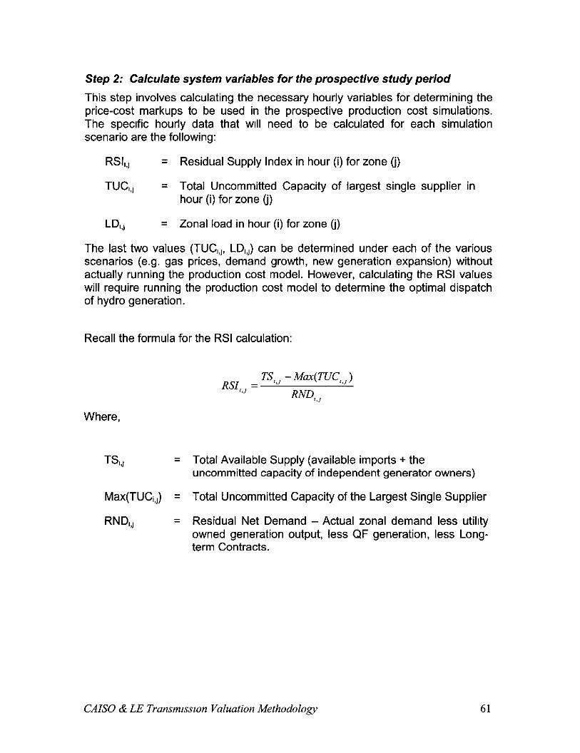
Step 2: Calculate system variables for the prospective study period
This step involves calculating the necessary hourly variables for determining the price-cost markups to be used in the prospective production cost simulations. The spectfic hourly data that WIII need to be calculated for each simulation scenario are the following:
RSI,,,
TUC,,,
= Residual Supply Index in hour (i) for zone (j)
= Total Uncommitted Capacity of largest single supplier in hour (i) for zone (j)
U,, = Zonal load in hour (i) for zone (j)
The last two values (TUC,,,, LD,,,) can be determined under each of the various scenarios (e.g. gas prices, demand growth, new generation expansion) without actually running the production cost model. However, calculating the RSI values will require running the production cost model to determine the optimal dispatch of hydro generation.
Recall the formula for the RSI calculation:
RSI = Ts,,, - M4TuC,,, 1 ‘.I
MDr,,
Where.
W,, = Total Available Supply (available imports + the uncommitted capacity of independent generator owners)
Max(TUCi,,) = Total Uncommitted Capacity of the Largest Single Supplier
RW,, = Residual Net Demand - Actual zonal demand less utikty owned generation output, less QF generation, less Long- term Contracts.
CAB0 & LE Transmwlon Valuation Methodology 61
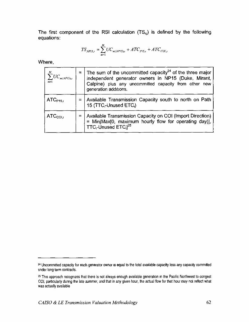
The first component of the RSI calculation (TS,,,) is defined by the following equations:
Where,
gJ~m,NP~s~.~ = The sum of the uncommitted capaciv4 of the three major
independent generator owners in NP15 (Duke, Mirant, Calpine) plus any uncommrtted capacity from other new generation addrtrons.
ATCprs,, = Available Transmission Capacity south to north on Path 15 (TTC,-Unused ETC,)
AT&,, = Available Transmission Capacity on COI (Import Direction) = Min[Max[O, maximum hourly flow for operating day)], TTC,-Unused ETC,]25
*b Uncommitted capacity for each generator owner IS equal to the total avallable capacity less any capacity commltted under long-term contracts.
25 This approach recogmzes that there is not always enough avaIlable generation in the Pacrflc Northwest to congest COI, parhcularly during the late summer, and that in any given hour, the actual flow for that hour may not reflect what was actually available
CAlSO & LE Transmission Valuation Methodology 62
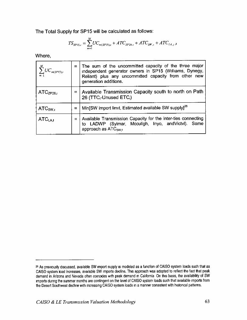
The Total Supply for SP15 will be calculated as follows:
T&m,, = &GsP,,,,, + AT%,,,, + ATC,,,, + A%, .I rn=l
Where,
= The sum of the uncommitted capacity of the three major Independent generator owners in SP15 (Wtlliams, Dynegy, Reliant) plus any uncommrtted capacity from other new generation additions.
ATcz~z6.1 = Available Transmission Capacity south to north on Path 26 (TTC,-Unused ETC,)
ATCsw.,
AT&
= Min[SW import limrt, Estimated available SW s~pply]~~
= Available Transmission Capacity for the inter-ties connecting to LADWP (Sylmar, Mccullgh, Inyo, andvictvl). Same approach as ATCsw,,
26 As prevrously drscussed, avallable SW Import supply IS modeled as a function of CAlSO system loads such that as CAlSO system load increases, avarlable SW Imports decline. Thus approach was adopted to reflect the fact that peak demand in Arizona and Nevada often corncrdes wrth peak demand tn Calrfornia On this basts, the availabikty of SW Imports durrng the summer months are contingent on the level of CAlSO system loads such that avarlable Imports from the Desert Southwest declrne wrth rncreasrng CAISO system loads rn a manner consrstent with htstorrcal patterns.
CAISO & LE Transmrssion Valuation Methodology 63
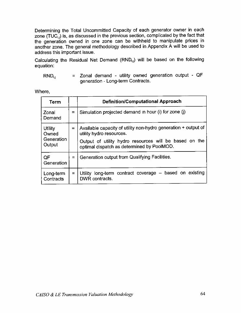
Determining the Total Uncommitted Capacity of each generator owner in each zone (TUC,,,) is, as discussed in the previous section, complicated by the fact that the generation owned in one zone can be withheld to manipulate prices in another zone. The general methodology described in Appendix A will be used to address this important issue.
Calculating the Residual Net Demand (RND,,,) will be based on the following equation: -
RND,,, =
Where,
Term
Zonal = Demand
Utility = Owned Generation output
QF = Generation
Long-term = Contracts
Zonal demand - utilrty owned generation output - QF generation - Long-term Contracts.
Definition/Computational Approach
Simulation projected demand In hour (i) for zone (j)
Available capacity of utility non-hydro generation + output of utility hydro resources.
Output of utility hydro resources will be based on the optimal dispatch as determined by PoolMOD.
Generation output from Qualifying Facilrties.
Utility long-term contract coverage - based on existing DWR contracts.
CAB0 & LE Transmission Valuation Methodology 64
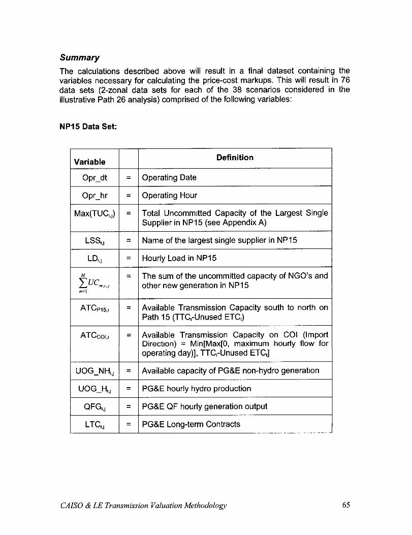
Summary The calculations described above will result in a final dataset containing the variables necessary for calculating the price-cost markups. This will result in 76 data sets (2-zonal data sets for each of the 38 scenarios considered in the illustrative Path 26 analysis) comprised of the following variables:
\ rlariable Definition
Opr-dt 1 = 1 Operating Date
Opr-hr 1 = 1 Operating Hour
I Vlax(TUC,,,) = I I Total Uncommrtted Capacity of the Largest Single Supplier in NP15 (see Appendix A)
LSS,,, 1 = 1 Name of the largest single supplier in NP15
LQ,, 1 = I Hourly Load in NP15
NPI 5 Data Set:
= The sum of the uncommitted capacrty of NGO’s and other new generatron in NP15
ATCPIS,, = Available Transmission Capacity south to north on Path 15 (TTC,-Unused ETC,)
ATCow = Available Transmission Capacity on COI (Import Directlon) = Min[Max[O, maximum hourly flow for operating day)], TTC,-Unused ETC,]
UOG-NH,,, 1 = I Available capacity of PG&E non-hydro generahon
UOG-H,,, I = I PG&E hourly hydro production
QW,, 1 = I PG&E QF hourly generation output
LX,, 1 = I PG&E Long-term Contracts
CAISO & LE Transmission Valuation Methodology 65

SP15 Data Set:
Variable Definition
Opr-dt = Operating Date
Opr-hr = Operating Hour
MaWG,) = Total Uncommitted Capacity of the Largest Single Supplier in SP15
LSS,,, = Name of the largest single supplier in SP15
Lb, = Hourly Load In SP15
g ucmh, = The sum of the uncommitted capacity of NGO’s and
other new generation in SP15
ATCZPZ~,, = Available Transmission Capacity south to north on Path 26 (TTC,-Unused ETC,)
AT&w,, = Mrn[SW Import limit, Estimated available SW supply
ATCLA,I = AvarIable Transmissron Capacity for the Inter-ties connecting to LADWP (Sylmar, Mccullgh, Inyo, andktvl). Same approach as AT&w,,
UOG-NH,,, = Available capacity of SCE & SDGE non-hydro generation
UOG-H,,, = SCE hourly hydro production
QFG,,, = SCE & SDGE QF hourly generation output
LTC,,, = SCE & SDGE Long-term Contracts
CAB0 & LE Transmxsion Vaiuatron Methodology 66
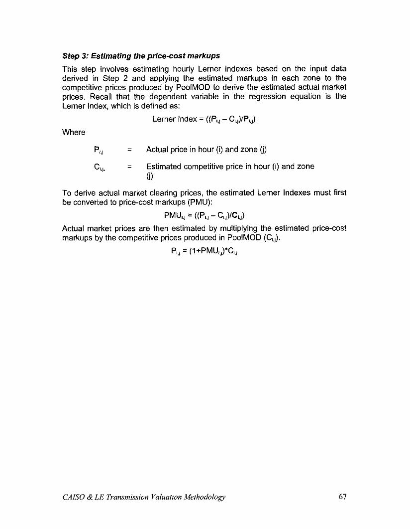
Step 3: Estimating the price-cost markups
This step involves estimating hourly Lerner indexes based on the input data derived in Step 2 and applying the estimated markups in each zone to the competitive prices produced by PoolMOD to derive the estimated actual market prices. Recall that the dependent variable in the regression equation is the Lerner Index, which is defined as:
Lerner Index = ((P,,, - C,,,)/P,,,)
Where
p,,, = Actual price in hour (i) and zone (j)
Cl,,, = Estimated competitive price in hour (I) and zone ti)
To derive actual market clearing prices, the estimated Lerner Indexes must first be converted to price-cost markups (PMU):
PMU,) = (0’l.l - ‘QGJ Actual market prices are then estimated by multiplying the estimated price-cost markups by the competitive prices produced in PoolMOD (C,,,).
P,,, = (1 +PMU,,,)*G,,
CAISO & LE Transmission Valuation Methodology

Step 4: Calculating new generation investment
An equilibrium new generation entry level will need to be calculated for the base case scenarios using the estimated actual market prices derived from the price- cost markups. This will be done by comparing the annual average unit revenues for a new combined cycle unit based on the prices derived in Step 3 to entry trigger prices that reflect the revenue requirements for a new combined cycle unit. If the annual average unit revenues exceed the trigger price, new generation will be added and steps 2, 3, and 4 will be repeated until no further entry is called for, as shown in Figure 24 below.
Figure 24. Process for Modeling New Generation Entry
Competltlve Prices and Input data for
regressjon analysis
L-
. . .
. . .
. . .
. . .
. . .
. . .
. . .
-
-I
AUTOMATED PROCESS
. . . , . . . ,,- ‘: ‘,’ . . . ). ; . . .
I ; / . . . I ‘: *-. .( L ,, -
Stop at Stop at prewous prewous
v v results results
9 No
Add new generatlon
CAISO & LE Transmission Valuation Methodology 68
IV. Selection of Scenarios In order to provide a comprehensive and accurate assessment of the economic benefits of a transmission expansion, the benefits must be examined under a wide range of system conditions. As discussed in previous sections, assumptions about natural gas prices, demand levels, hydro conditions, and new generation entry can have significant impacts on the economic benefits of a transmission expansion. The benefits of a transmission expansion should be examined under different plausible combinations of these system variables. In choosing scenarios, it is particularly import to capture extreme scenarios, such as combinatrons of high demand and low hydro conditions, because the benefits of a transmission expansion can often be significantly higher under extreme system condrtions. It is also Important to choose a sufficient number of more moderate scenarios to ensure the benefits are accurately captured under more likely scenarios. There is no hard rule on the number of scenarios that ought to be considered other than “more is always better”. Ultimately, the number of scenarios considered IS likely to be driven by practical issues such as the amount of the time one has to undertake a study and the speed at which scenarios can be run and results compiled.
In this section we provide a two-step methodology for selecting scenarios that provides a means for ensuring extreme scenarios are included in the assessment and that a representative sample of more moderate scenarios are also selected. In the first step, the most likely as well as some extreme scenarios are pre- selected. In addition, scenarios are selected where only on for different values of a particular market variable holding all other choice variables constant. This sampling technique allows one to isolate the effects a single variable has on the estimated benefits. In the second step, additional scenarios are randomly selected using a technique referred to as “Latin Hypercube Sampling”. The first step ensures the more interesting and important scenarios are considered (e.g. extreme and most likely). The second step ensures a representative sample of all possible scenarios.
This two-step approach was used to select scenarios for demand levels and natural gas prices in the illustrative analysis of Path 26 and is described in detail below. The methodology used to select long-term new generation entry scenarios and hydro scenarios is also discussed.
CAISO & LE Transmmion Valuation Methodology 69
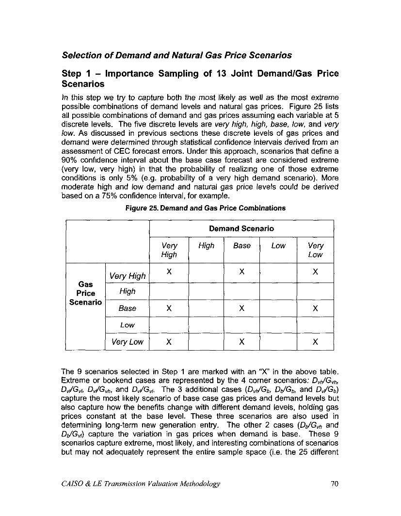
Selection of Demand and Natural Gas Price Scenarios
Step 1 - Importance Sampling of 13 Joint Demand/Gas Price Scenarios In this step we try to capture both the most likely as well as the most extreme possible combinations of demand levels and natural gas prices. Figure 25 lists all possible combinations of demand and gas prices assuming each variable at 5 discrete levels. The five discrete levels are very high, high, base, low, and very low. As discussed in previous sectrons these drscrete levels of gas prices and demand were determined through statistical confidence intervals derived from an assessment of CEC forecast errors. Under this approach, scenarios that define a 90% confidence interval about the base case forecast are considered extreme (very low, very high) in that the probability of realizrng one of those extreme conditions is only 5% (e.g. probability of a very high demand scenario). More moderate high and low demand and natural gas price levels could be derived based on a 75% confidence interval, for example.
Figure 25. Demand and Gas Price Combinations
Gas Price
Scenario
Demand Scenario
The 9 scenarios selected in Step 1 are marked with an “x” in the above table. Extreme or bookend cases are represented by the 4 corner scenarios: D,dG,*, D,JGvr, DVJGVh, and D,JGvr. The 3 additional cases (DvIJGb, DdGb, and D,JGb) capture the most kkely scenario of base case gas prices and demand levels but also capture how the benefits change with different demand levels, holding gas prices constant at the base level. These three scenarios are also used in detem-rining long-term new generation entry. The other 2 cases (&/G,h and DdGyl) capture the variation in gas prices when demand is base. These 9 scenarios capture extreme, most likely, and interesting combinations of scenarios but may not adequately represent the entire sample space (i.e. the 25 different
CAB0 & LE Transmission Valuation Methodology 70
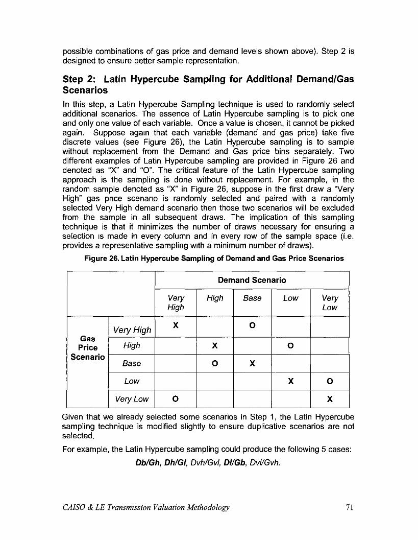
possible combinations of gas price and demand levels shown above). Step 2 is designed to ensure better sample representation.
Step 2: Latin Hypercube Sampling for Additional Demand/Gas Scenarios In this step, a Latin Hypercube Sampling technique is used to randomly select additional scenarios. The essence of Latin Hypercube sampling is to pick one and only one value of each variable. Once a value is chosen, it cannot be picked again. Suppose agarn that each variable (demand and gas price) take five discrete values (see Figure 26) the Latin Hypercube sampling is to sample without replacement from the Demand and Gas price bins separately. Two different examples of Latin Hypercube sampling are provided in Figure 26 and denoted as “X” and “0”. The critical feature of the Latin Hypercube sampling approach is the sampling is done without replacement. For example, in the random sample denoted as “x” in Figure 26, suppose in the first draw a “Very High” gas price scenario is randomly selected and paired with a randomly selected Very High demand scenario then those two scenarios will be excluded from the sample in all subsequent draws. The implication of this sampling technique is that it minimizes the number of draws necessary for ensuring a selection IS made in every column and in every row of the sample space (i.e. provides a representative sampling with a minimum number of draws).
Figure 26. Latin Hypercube Sampling of Demand and Gas Price Scenarios
Given that we already selected some scenarios in Step 1, the Latin Hypercube sampling technique is modified slightly to ensure duplicative scenarios are not selected.
For example, the Latin Hypercube sampling could produce the following 5 cases:
Db/Gh, Dh/GI, Dvh/Gvl, DMGb, DvVGvh.
CAB0 & LE Transmission Valuation Methodology 71
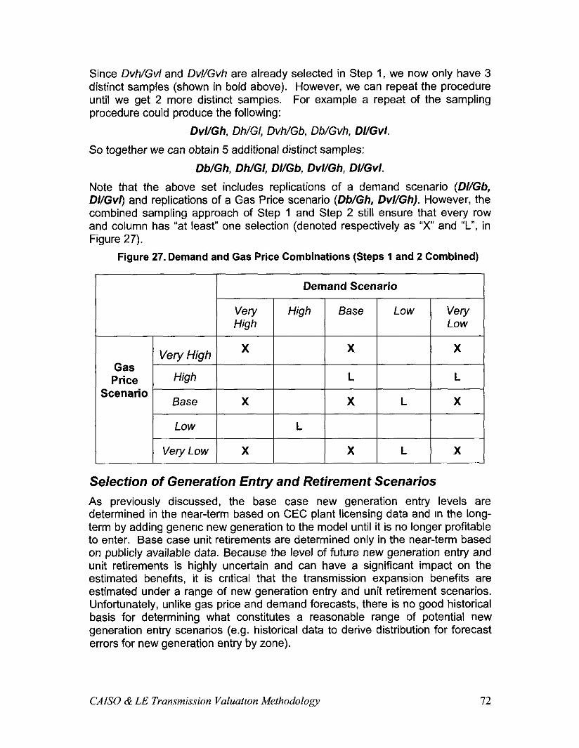
Since DvWGvl and Dv//Gvh are already selected in Step 1, we now only have 3 distinct samples (shown in bold above). However, we can repeat the procedure until we get 2 more distinct samples. For example a repeat of the sampling procedure could produce the following:
DvVGh, Dh/GI, Dvh/Gb, Db/Gvh, DMGvI.
So together we can obtain 5 additional distinct samples:
Db/Gh, Dh/GI, DI/Gb, DWGh, DI/Gvl.
Note that the above set includes replications of a demand scenario (D//Gb, D//G@ and replications of a Gas Price scenario (Db/Gh, Dv//Gh). However, the combined sampling approach of Step 1 and Step 2 still ensure that every row and column has “at least” one selection (denoted respectively as “x” and ‘I”, in Figure 27).
Figure 27. Demand and Gas Price Combinations (Steps 1 and 2 Combined)
Very High ’ X X Gas
Price High L L Scenario
Base X X L X
Low L
VeryLow X X L X
Selection of Generation Entry and Retirement Scenarios As previously discussed, the base case new generation entry levels are determined in the near-term based on CEC plant licensing data and In the long- term by adding generic new generation to the model until it is no longer profitable to enter. Base case unit retirements are determined only in the near-term based on publicly available data. Because the level of future new generation entry and unit retirements is highly uncertain and can have a significant impact on the estimated benefits, it is critical that the transmission expansion benefits are estimated under a range of new generation entry and unit retirement scenarios. Unfortunately, unlike gas price and demand forecasts, there is no good historical basis for determining what constitutes a reasonable range of potential new generation entry scenarios (e.g. historical data to derive distribution for forecast errors for new generation entry by zone).
CAISO & LE Transmission Valuatron Methodology 72

Given the lack of historical data, it is important to conduct sensitivity analysis for a wide range of new generation entry scenarios. In the illustrative Path 26 analysis, sensitivity analysis was conducted around the base case “long-term” new generation entry level” using approximately +/- 50 % of baseline annual incremental entry levels to capture over and under entry conditions. Under this approach 3 possible new generation entry scenarios were considered for each zone (Over-entry = “O”, Normal or base-case entry = “N”, and Under-entry = “U”). With three zones and three possible entry scenarios for each zone, a total of 27 different entry combinations are possible. Combined zonal new generation entry scenarios are labeled in the following order (NP15, ZP26, SP15). For example, a new generation entry scenario labeled “ONU” would represent over-entry in NP15, normal entry in ZP26, and under-entry in SP15.
Ideally, the 2-step sampling approach described above for sampling demand and natural gas price scenarios should be applied to the 27 new generation entry scenarios. Under thus approach, interesting new generation entry scenarios, such as the most likely scenarios and the scenarios that are likely to minimize or maximize the benefits of a transmission expansion would be preselected and then additional scenarios would be selected using the Step 2 Latin Hypercube sampling approach. The approach would be exactly analogous to the demand and gas price scenario selection except that instead of the sample space being 2-dimensional, it would be 3-dimensional (i.e. a 3X3 cube where each zone is a dimension consisting of 3-categories (over-entry, normal entry, under-entry). Applying the Latin Hypercube sampling approach to a 3X3 cube would result in 9 unique scenarios (i.e. there would be a unique selectron from every row and column in the entire cube). These g-scenarios would then be combined with the interesting scenarios selected in Step 1.
While this would be the preferred approach to sampling new generation entry scenarios, given the time limitations and the practical necessity of needing to limit the sample selectron to a manageable size only some interesting new generation entry scenarios were considered in the illustrative Path 26 analysis. Specifically, three scenarios were considered, the most likely scenario of normal entry in all three zones (NNN), a scenario of under-entry in NP15 and SP15 and over-entry in ZP26 (UOU), and a scenario of over-entry in NP15 and SP15 and under-entry in ZP26 (OUO).
The various selected demand, gas price, and new generation entry levels results in a total of 84 scenarios (2-transmission investment options (“Path 26 expansion” and “No expansion”), 14-demand and gas scenarios, and 3-zonal new generation entry scenarios). Given the time limitations and the practical necessity of needing to limit the sample selection to a manageable size, a subset of 38 scenarios (19 for each transmission expansion option) was selected. This subset, which is shown below in Figure 28, was selected to capture both
27 The base case level IS the level dewed from lteratrvely addlng block Increments of generic new generatlon to the model in each zone until market revenues were lnsuffuent to support any addItIonal entry.
CAISO & LE Transmission Valuation Methodology 13
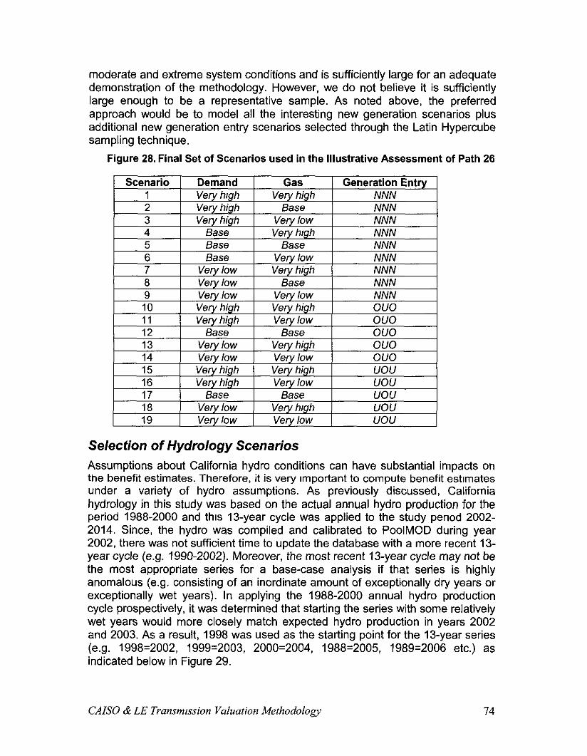
moderate and extreme system conditions and is sufficiently large for an adequate demonstration of the methodology. However, we do not believe it is sufficiently large enough to be a representative sample. As noted above, the preferred approach would be to model all the interesting new generation scenarios plus additional new generation entry scenarios selected through the Latin Hypercube sampling technique.
Figure 28. Final Set of Scenarios used in the Illustrative Assessment of Path 28
Scenario Demand 1 Gas ) Generation Entry 1 Vefyhrgh 1 Very high 1 hlhlhl , ., ., . 2
1 verynnrgn 1 Base NNN 3 I,.~.. L..~~I very “IQ” , I,-~- ,-... very IOW NNN 4 Base I Vwv hroh . _, NNN 5 Base I -~~~ aase I AlAlA, - 6 Base \/mv Imu 7 Very low very mgn 1 8 Very low Rs‘?e I
.,
,111,”
-I. .-.. I NNN , ., ,.,~ / NNN
Y I very low In I %I_-. L:..L
I ---” NNN Very low NNN
I I,--. LZ-L ouo I Very low ouo
-~ ouo r\, m
1 --- UOU
I n___ Base UOU
Very low 1 very IOW Very high ) Very high Vwv hioh 1 verv low
Lmse Very low Very/low I very IOW I
14 15 16 17 18 19
Selection of Hydrology Scenarios Assumptions about California hydro conditions can have substantial impacts on the benefit estimates. Therefore, it is very Important to compute benefit estimates under a variety of hydro assumptions. As previously discussed, California hydrology in this study was based on the actual annual hydro production for the period 1988-2000 and this 13-year cycle was applied to the study period 2002- 2014. Since, the hydro was compiled and calibrated to PoolMOD during year 2002, there was not sufficient time to update the database with a more recent 13- year cycle (e.g. 1990-2002). Moreover, the most recent 13-year cycle may not be the most appropriate series for a base-case analysis if that series is highly anomalous (e.g. consisting of an inordinate amount of exceptionally dry years or exceptionally wet years). In applying the 1988-2000 annual hydro production cycle prospectively, it was determined that starting the series with some relatively wet years would more closely match expected hydro production in years 2002 and 2003. As a result, 1998 was used as the starting point for the 13-year series (e.g. 1998=2002, 1999=2003, 2000=2004, 1988=2005, 1989=2006 etc.) as indicated below in Figure 29.
CAB0 & LE Transmwion Valuation Methodology 74
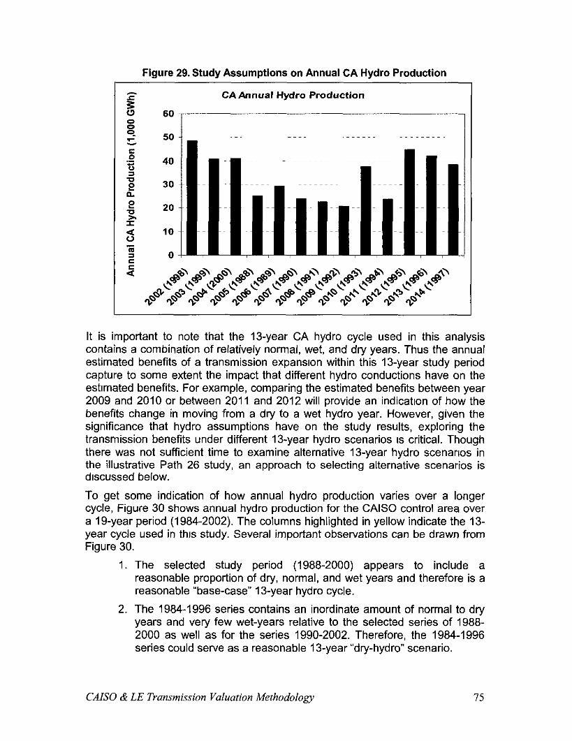
Figure 29. Study Assumptions on Annual CA Hydro Production
I g CA Annual Hydra Production
60
50
It is important to note that the 13-year CA hydro cycle used in this analysis contains a combination of relatively normal, wet, and dry years. Thus the annual estimated benefits of a transmission expansron within this 13-year study period capture to some extent the impact that different hydro conductions have on the estrmated benefits. For example, comparing the estimated benefits between year 2009 and 2010 or between 2011 and 2012 will provide an indicatron of how the benefits change in moving from a dry to a wet hydro year. However, given the significance that hydro assumptions have on the study results, exploring the transmission benefits under different 15year hydro scenarios IS critical. Though there was not sufficient time to examine alternative 13-year hydro scenarios in the illustrative Path 26 study, an approach to selecting alternative scenarios is discussed below.
To get some indication of how annual hydro production varies over a longer cycle, Figure 30 shows annual hydro production for the CAISO control area over a 19-year period (1984-2002). The columns highlighted in yellow indicate the 13- year cycle used in this study. Several important observations can be drawn from Figure 30.
1. The selected study period (1988-2000) appears to include a reasonable proportion of dry, normal, and wet years and therefore is a reasonable “base-case” 13-year hydro cycle.
2. The 1984-1996 series contains an inordinate amount of normal to dry years and very few wet-years relative to the selected series of 1988- 2000 as well as for the series 1990-2002. Therefore, the 1984-1996 series could serve as a reasonable 13-year “dry-hydro” scenario.
CAISO & LE Transmission Valuation Methodology 15
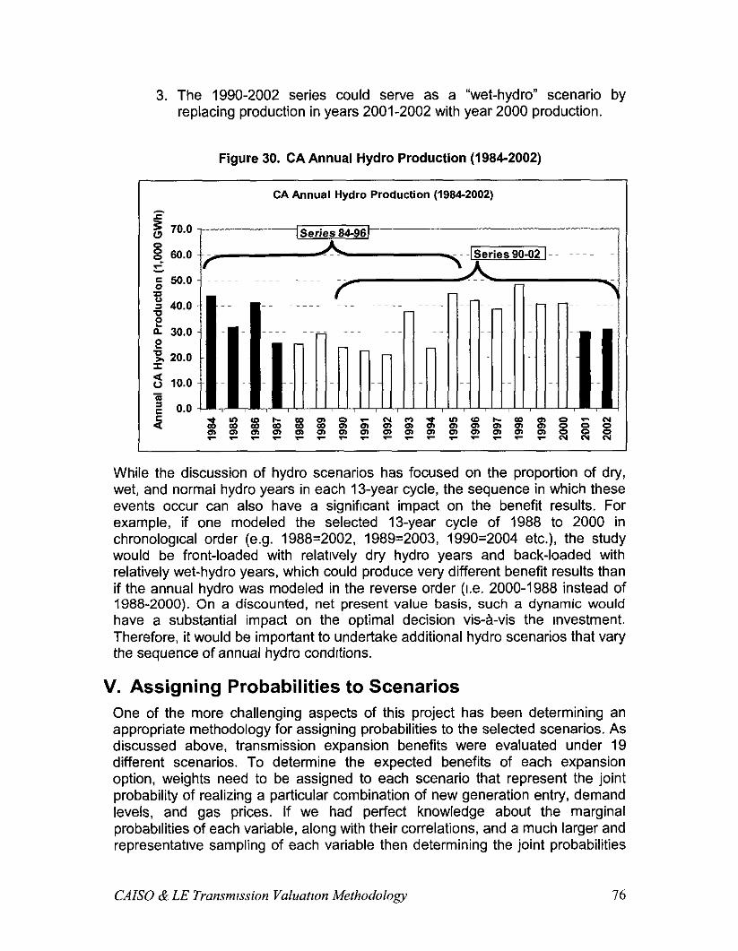
3. The 1990-2002 series could serve as a “wet-hydro” scenario by replacing production in years 2001-2002 with year 2000 production.
Figure 30. CA Annual Hydro Production (1984-2002)
CA Annual Hydro Production (1964-2002)
lZ 5 70.0 0 x 60.0 5 c
2 50.0
ti 4 40.0
2 = 30.0 e
z 20.0
s 10.0 Z = 0.0
c rzr.-.-.-rrNeIN
While the discussion of hydro scenarios has focused on the proportion of dry, wet, and normal hydro years in each 13-year cycle, the sequence in which these events occur can also have a significant impact on the benefit results. For example, if one modeled the selected 13-year cycle of 1988 to 2000 in chronologtcal order (e.g. 1988=2002, 1989=2003, 1990=2004 etc.), the study would be front-loaded with relatively dry hydro years and back-loaded with relatively wet-hydro years, which could produce very different benefit results than if the annual hydro was modeled in the reverse order (I.e. 2000-1988 instead of 1988-2000). On a discounted, net present value basis, such a dynamic would have a substantial impact on the optimal decision vis-a-vis the investment. Therefore, it would be important to undertake additional hydro scenarios that vary the sequence of annual hydro conditions.
V. Assigning Probabilities to Scenarios One of the more challenging aspects of this project has been determining an appropriate methodology for assigning probabilities to the selected scenarios. As discussed above, transmission expansion benefits were evaluated under 19 different scenarios. To determine the expected benefits of each expansion option, weights need to be assigned to each scenario that represent the joint probability of realizing a particular combination of new generation entry, demand levels, and gas prices. If we had perfect knowledge about the marginal probabilities of each variable, along with their correlations, and a much larger and representative sampling of each variable then determining the joint probabilities
CAB0 & LE Transmnsion Valuatron Methodology 16

of realizing particular combinations of these variables would be very straightforward. Unfortunately, we do not have perfect knowledge about the marginal probabilities of each variable nor do we have a sufficient sample size to claim that we have representative sampling. Consequently, an alternative approach to determining the joint probabilities of each scenario is needed.
The approach adopted here is a 2-stage approach that consists of an approach advocated by Ben Hobbs (Stage 1) and an approach advocated by Frank Wolak (Stage 2) both of whom are members of the IS0 Market Surveillance Committee. In the first stage, joint probabilities are derived for the various combinations of gas price and demand levels. These joint probabilities are then used in a second stage to determine the joint probability of the pairs of gas price and demand levels and the new generation entry scenarios28. This 2-stage approach was driven by the fact that we have much better information on the probability distributions of demand and gas prices than we do on the level of new generation entry. Each of these stages is described in greater detail below.
28 The second stage could also be used to ass!gn probabrlitles to various hydra scenarios Thus was not done In thus study because trme did not permit the evaluation of alternative hydro scenarios
CAB0 & LE Transmission Valuatmn Methodology 77
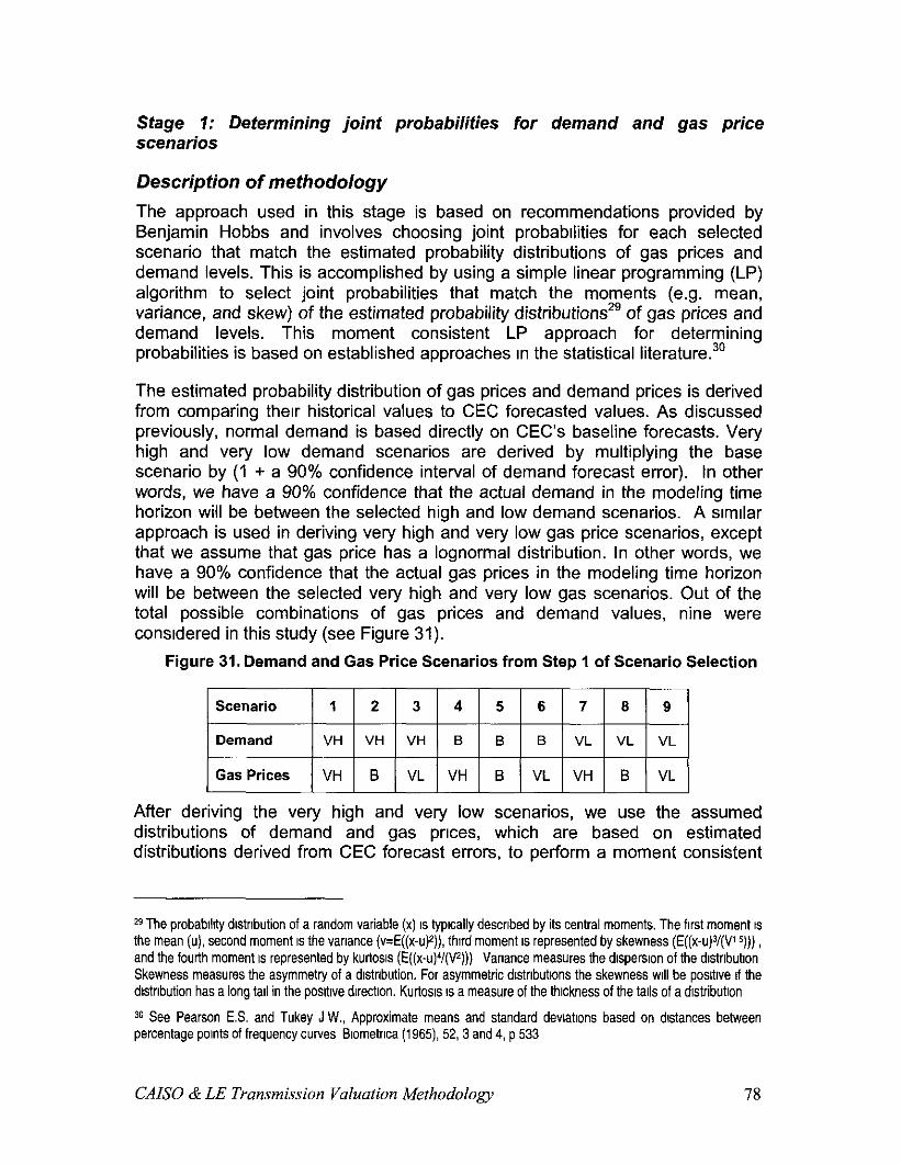
Stage 1: Determining joint probabilities for demand and gas price scenarios
Description of methodology
The approach used in this stage is based on recommendations provided by Benjamin Hobbs and involves choosing joint probabilities for each selected scenario that match the estimated probability distributions of gas prices and demand levels. This is accomplished by using a simple linear programming (LP) algorithm to select joint probabilities that match the moments (e.g. mean, variance, and skew) of the estimated probability distributions” of gas prices and demand levels. This moment consistent LP approach for determining probabilities is based on established approaches In the statistical literature.30
The estimated probability distribution of gas prices and demand prices is derived from comparing therr historical values to CEC forecasted values. As discussed previously, normal demand is based directly on CEC’s baseline forecasts. Very high and very low demand scenarios are derived by multiplying the base scenario by (1 + a 90% confidence interval of demand forecast error). In other words, we have a 90% confidence that the actual demand in the modeling time horizon will be between the selected high and low demand scenarios. A srmilar approach is used in deriving very high and very low gas price scenarios, except that we assume that gas price has a lognormal distribution. In other words, we have a 90% confidence that the actual gas prices in the modeling time horizon will be between the selected very high and very low gas scenarios. Out of the total possible combinations of gas prices and demand values, nine were considered in this study (see Figure 31).
Figure 31. Demand and Gas Price Scenarios from Step 1 of Scenario Selection
Scenario 1 2 3 4 5 6 7 8 9
Demand VH VH VH B B B VL VL VL
Gas Prices VH B VL VH B VL VH B VL
After deriving the very high and very low scenarios, we use the assumed distributions of demand and gas prices, which are based on estimated distributions derived from CEC forecast errors, to perform a moment consistent
2g The probablkty drstrrbution of a random variable (x) IS typrcally described by its central moments. The first moment IS the mean (u), second moment IS the variance (v=E((x-u)*)), third moment IS represented by skewness (E((x-u)3/(V15))) , and the fourth moment IS represented by kurtosls (E((x-u)Y(V2))) Varrance measures the drsperslon of the drstrlbutron Skewness measures the asymmetry of a drstnbution. For asymmetric drstrrbutlons the skewness wrll be posrtwe if the drstrrbution has a long tall in the posltrve dIrectIon. Kurlos~s IS a measure of the thtckness of the tails of a drstributron
30 See Pearson ES and Tukey J W., Approximate means and standard dewatlons based on drstances between percentage points of frequency curves Blometrlca (1965), 52, 3 and 4, p 533
CAISO & LE Transmission Valuation Methodology 18

LP approach to derive the joint probabilities of demand/gas prices by minimizing the sum of the squared joint probabilities3’ and the sum of the squared third moments of the marginal demand and gas price distributions subject to the constraints of matching the mean and variance of these distributions and that the joint probabilities sum to 1. More specifically, we solve the following LP problem, supposing there are m unrque demand/gas price scenarios:
3’ Minimung the joint probabllrties subject to the constraint that they sum to one mitigates against extreme solutions where some scenarios have a wght close to zero and other scenarios have a weight close to 1
CAB0 & LE Transmission Valuation Methodology 19
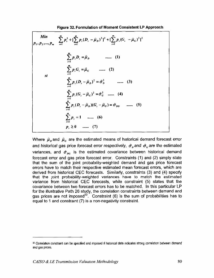
Figure 32. Formulation of Moment Consistent LP Approach
Min
‘1 9 P* 9.9 Pm Tp: +1@(D, -&)‘I2 +@m -ml’ ,=I
PJ’, =I% . . . . . . (1)
; P&G, =Pc . . . . . . (2)
~P,(D, -ii,)’ =6:, ,=I
. . . . . . (3)
Tp,(G, -&)’ =6 . . . . . . (4) ,=I
gp,(D, -P,)(G, -&) =&oc . . . . . . (5) x=1
g P, = 1 . . . . . . (6)
P, 20 . . . . . . (7)
Where P,and & are the estimated means of historical demand forecast error and historical gas price forecast error respectively, 8, and aG are the estimated variances, and Sot is the estimated covariance between historical demand forecast error and gas price forecast error. Constraints (1) and (2) simply state that the sum of the joint probability-weighted demand and gas price forecast errors have to match their respective estimated mean forecast errors, which are derived from historical CEC forecasts. Similarly, constraints (3) and (4) specify that the joint probability-weighted variances have to match the estimated variance from historical CEC forecasts, while constraint (5) states that the covariance between two forecast errors has to be matched. In this particular LP for the illustrative Path 26 study, the correlation constraints between demand and gas prices are not imposed3’. Constraint (6) is the sum of probabilities has to equal to 1 and constraint (7) is a non-negativity constraint.
32 Correlation constramt can be specified and Imposed 11 hlstorlcal data mdlcates strong correlation between demand and gas prices.
CAISO & LE Transmission Valuatron Methodology 80
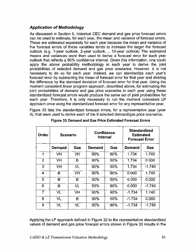
Application of Methodology As discussed In Section II, historical CEC demand and gas price forecast errors can be used to estimate, for each year, the mean and variance of forecast errors. These are estimated separately for each year because the mean and variance of the forecast errors of these variables tends to increase the larger the forecast outlook (e.g. l-year outlook, 2-year outlook, 13-year outlook) The estimated means and variances were then used to derive a forecast error for each year outlook that reflects a 90% confidence interval. Given this information, one could apply the above probability methodology in each year to derive the joint probabilities of selected demand and gas price scenarios. However, it is not necessary to do so for each year. Instead, we can standardize each year’s forecast error by subtracting the mean of forecast error for that year and dividing the difference by the standard deviation of forecast error for that year. Using the moment consistent linear program approach, described above, for estimating the joint probabilrties of demand and gas price scenarios in each year using these standardized forecast errors would produce the same set of joint probabilities for each year. Therefore, it is only necessary to run the moment consrstent LP approach once using the standardized forecast error for any representative year.
Figure 33 lists the standardized forecast errors, for a representative year (year 4) that were used to derive each of the 9 selected demand/gas price scenarios.
Figure 33. Demand and Gas Price Estimated Forecast Errors
Order Scenario Confidence Interval
Standardized Estimated
Forecast Error
Applying the LP approach defined in Figure 32 to the representative standardized values of demand and gas price forecast errors shown in Figure 33 results in the
CAB0 & LE Transmission Valuation Methodology 81
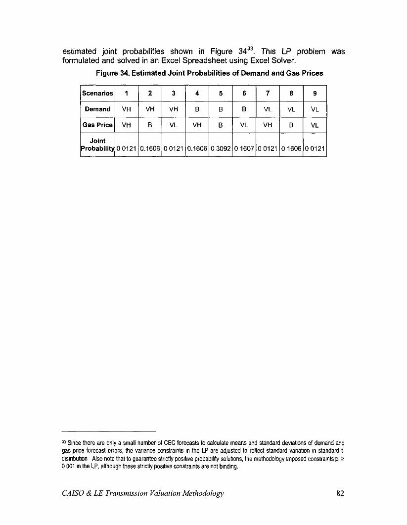
estimated joint probabilities shown in Figure 3433. This LP problem was formulated kd solved in an Excel Spreadsheet using Excel Solver..
Figure 34. Estimated Joint Probabilities of Demand and Gas Prices
33 Since there are only a small number of CEC forecasts to calculate means and standard devlabons of demand and gas price forecast arrors, the variance constraints In the LP are adjusted to reflect standard varlatlon In standard t- dlstrlbubon Also note that to guarantee strictly poslbve probablllty solubons, the methodology Imposed constraints p, t 0 001 In the LP, although these strictly posrtive constralnts are not bIndIng.
CAB0 & LE Transmission Valuation Methodology 82
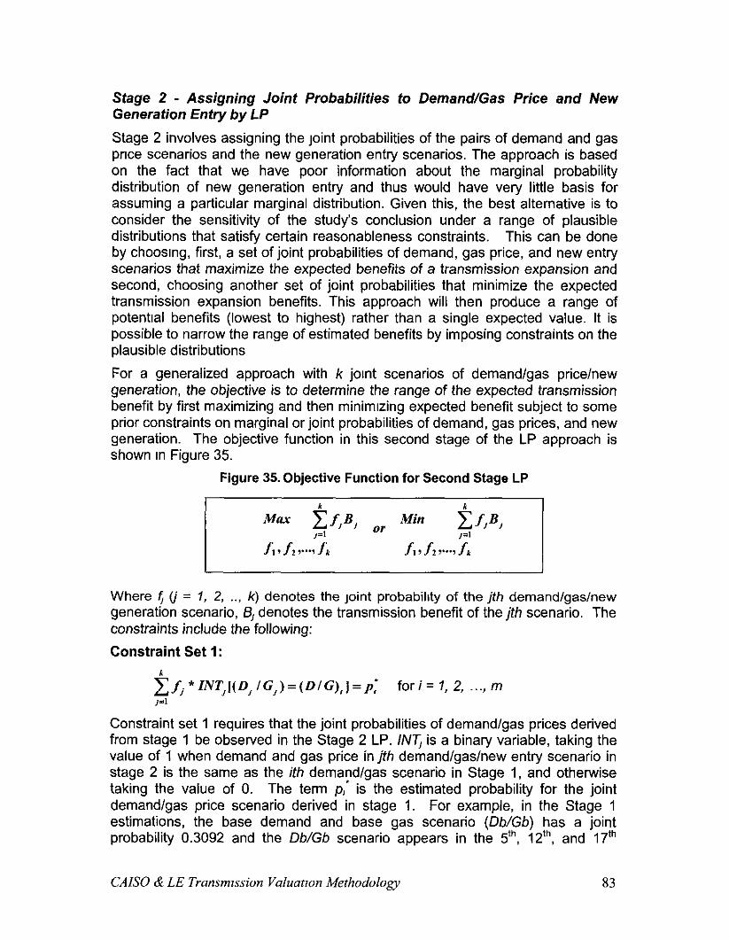
Stage 2 - Assigning Joint Probabilities to Demand/Gas Price and New Generation Entry by LP
Stage 2 involves assigning the joint probabilities of the pairs of demand and gas price scenarios and the new generation entry scenarios. The approach is based on the fact that we have poor information about the marginal probability distribution of new generation entry and thus would have very little basis for assuming a particular marginal distribution. Given this, the best alternative is to consider the sensitivity of the study’s conclusion under a range of plausible distributions that satisfy certain reasonableness constraints. This can be done by choosrng, first, a set of joint probabilities of demand, gas price, and new entry scenarios that maximize the expected benefits of a transmission expansion and second, choosing another set of joint probabilities that minimize the expected transmission expansion benefits. This approach will then produce a range of potentral benefits (lowest to highest) rather than a single expected value. It is possible to narrow the range of estimated benefits by imposing constraints on the plausible distributions
For a generalized approach with k jotnt scenarios of demand/gas price/new generation, the objective is to determine the range of the expected transmission benefit by first maximizing and then minimrzing expected benefit subject to some prior constraints on marginal or joint probabilities of demand, gas prices, and new generation. The objective function in this second stage of the LP approach is shown in Figure 35.
Figure 35. Objective Function for Second Stage LP
Where 4 (j = 7, 2, .., k) denotes the joint probabilrty of the #II demand/gas/new generation scenario, 13, denotes the transmission benefit of the J/I scenario. The constraints include the following:
Constraint Set 1:
$fi *ZlVT,[(D,/G,)=(DlG),]=p~ fori= 7, 2, _.., m
Constraint set 1 requires that the joint probabilities of demand/gas prices derived from stage 1 be observed in the Stage 2 LP. /NT, is a binary variable, taking the value of 1 when demand and gas price in jfh demand/gas/new entry scenario in stage 2 is the same as the it/~ demand/gas scenario in Stage 1, and otherwise taking the value of 0. The term p,’ is the estimated probability for the joint demand/gas price scenario derived in stage 1. For example, in the Stage 1 estimations, the base demand and base gas scenario (/X/G/J) has a joint probability 0.3092 and the Db/Gb scenario appears in the 5th, 12’h, and 17’h
CAB0 & LE Transmxkm Valuatron Methodology 83
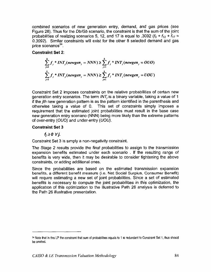
combined scenarios of new generation entry, demand, and gas prices (see Figure 28). Thus for the Db/Gb scenario, the constraint is that the sum of the joint probabilities of realizing scenarios 5, 12, and 17 is equal to .3092 (fs + f,z + fi7 = 0.3092). Similar constraints will exist for the other 8 selected demand and gas price scenartos34.
Constraint Set 2:
t f, * ZNTj(newgen, = NNN) 2 t f, * ZNT,(newgen, = OUO) j=l ,=I
2 f, * ZNT,(newgen, = NNN) 2 2 fj * ZNT,(newgen, = UOU) ,=I ,=I
Constraint Set 2 imposes constraints on the relative probabilities of certain new generation entry scenarios. The term /NT, is a binary variable, taking a value of 1 if the jfb new generation pattern is as the pattern identified in the parenthesis and otherwise taking a value of 0. This set of constraints simply imposes a requirement that the estimated joint probabilities must result in the base case new generation entry scenario (NNN) being more likely than the extreme patterns of over-entry (OUO) and under-entry (UOU).
Constraint Set 3
Constraint Set 3 is srmply a non-negativity constraint.
The Stage 2 results provide the final probabilities to assign to the transmission expansion benefits estimated under each scenario If the resulting range of benefits is very wide, then it may be desirable to consider tightening the above constraints, or adding additional ones.
Since the probabilities are based on the estimated transmission expansion benefits, a different benefit measure (i.e. Net Social Surplus, Consumer Benefit) will requrre estimating a new set of joint probabilities. Since a set of estimated benefits is necessary to compute the joint probabilities in this optimization, the applicatron of this optimization to the illustrative Path 26 analysis is deferred to the Path 26 illustrative presentation.
34 Note that in this LP the constramt that sum of probabilibes equals to 1 IS redundant to Constraint Set 1, thus should be omened.
CAISO & LE Transmusion Valuation Methodology 84

VI. Measuring Net-Benefits
Introduction In this section, we review the theory that underpins investment project evaluation, with a view to identifying the appropriate objective function or functions for the transmission valuation methodology. The section commences with a brief description of the optimal investment rule. It then sets out the principles of cost benefit analysis.
The optimal investment rule The optimal investment rule requires that in order to recommend a particular transmission investment, the IS0 must ensure that each candidate investment satisfies a two-part test, namely:
. social benefits of the transmission investment outweigh the social costs of the investment; and
l the transmission investment delivers the highest net social surplus, being the ratio of social benefit to socral cost.
The second part of the test implies that social welfare WIII only be maximized if the CAISO reviews the range of alternative projects that could substitute for the proposed transmission project, and rejects the proposed project if any one of them yields a greater social surplus. As a matter of practice, the CAISO can only address the second part of the test somewhat narrowly by reviewing:
. alternative timing choices or other transmission projects that might substitute for the proposed project; and
l whether generation or demand side management measures might negate the social benefits of the project.
Hence, as a practical matter, the CAISO will generally need to confine its analysrs to the first part of the test (whether the project yields net benefits), and address the second part of the test in the development of future market forecasts including the evaluation of the impacts of uncertainty therern. The remainder of this section proceeds on the basis that the principal task is to determine whether or not candidate transmission projects yield positive net benefits. This question is normally addressed through cost-benefit analysis.
Overview Cost-benefit analysis (CBA) is a widely used procedure for investigating whether a proposed project is desirable from a societal welfare standpoint. In customary practice, CBA implies approval of the project if its net present value exceeds
CAISO & LE Transmission Valuatron Methodology 85
zero, with all relevant benefits and costs over the projects lifetime factored into the calculation.35 This can be expressed mathematically as:
NPV = B, -co B, -c, *, - C, (l+d)O +(l+d)‘+-+(I+#
>o
where the subscripts represent periods from project initiation, d embodies a social discount rate and B and C represent benefits and costs respectively.
Alternatrvely, net benefits can be conceptualized as the summation across market partrcipants of their willingness to pay for the project, less the opportunity cost that reflects the benefits foregone due to implementing the project. Since most projects will enhance the welfare of some market participants while diminishing the welfare of others, practitioners of CBA often employ the Kaldor- Hicks criterion to judge the acceptability of an undertaking’s impact on society in aggregate. This principle holds that a project is supportable if the winners could theoretically compensate the losers for their decreased utility while maintaining a net welfare gain for themselves. In other words, the project must be Pareto- improving36 when the potential for transfer payments is factored in. Note that this criterion does not imply that redistribution must occur in reality, and in fact such transfers could modify the behavror of individual agents such that the efficiency gains resulting from the project would be partially offset.
Producer and consumer surplus as measures of benefit The Kaldor-Hicks criterion introduces the idea of winners and losers. Consumers win if they receive a lower price, which translates into an increased consumer surplus (being the difference between their willingness to pay and the price of the good). Producers win if they increase profits, which translates into an increased producer surplus (being the difference between the price of the good and the cost of its production). This is illustrated in Figure 36. Hence, if the sum of the changes in consumer and producer surplus consequent on the investment IS in excess of the cost of the investment, then the project must be (potentially) Pareto-improving and it should go ahead. The sum of the producer and consumer surplus in each period corresponds to the term (B-C) in equation (1) above.
35 Another approach developed by Keynes wolves determmlng the economic rate of return (ERR) that equates the tnltlal project cost with the sum of discounted future net benefits Thus method WIN deliver slmllar results when the Input assumptions are slmllar
s6 A change IS regarded as ‘Pareto-lmprowng’ I no one is made worse off but at least one person IS better off
CAISO & LE Transmzssion Valuatron Methodology 86
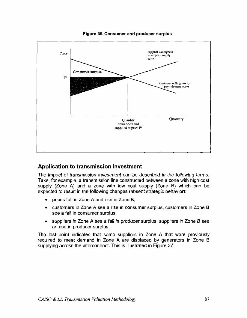
Figure 36. Consumer and producer surplus
/ Quanhty
demanded and supplEd at price P’
Quanhty
Application to transmission investment The impact of transmission investment can be described in the following terms. Take, for example, a transmission line constructed between a zone with high cost supply (Zone A) and a zone with low cost supply (Zone 6) which can be expected to result in the following changes (absent strategic behavior):
l prices fall in Zone A and rise in Zone B;
l customers in Zone A see a rise In consumer surplus, customers in Zone B see a fall in consumer surplus;
l suppliers in Zone A see a fall in producer surplus, supplrers in Zone B see an rise in producer surplus.
The last point indicates that some suppliers in Zone A that were previously required to meet demand in Zone A are displaced by generators in Zone B supplying across the Interconnect. This is illustrated in Figure 37.
CAISO & LE Transmission Valuation Methodology 87
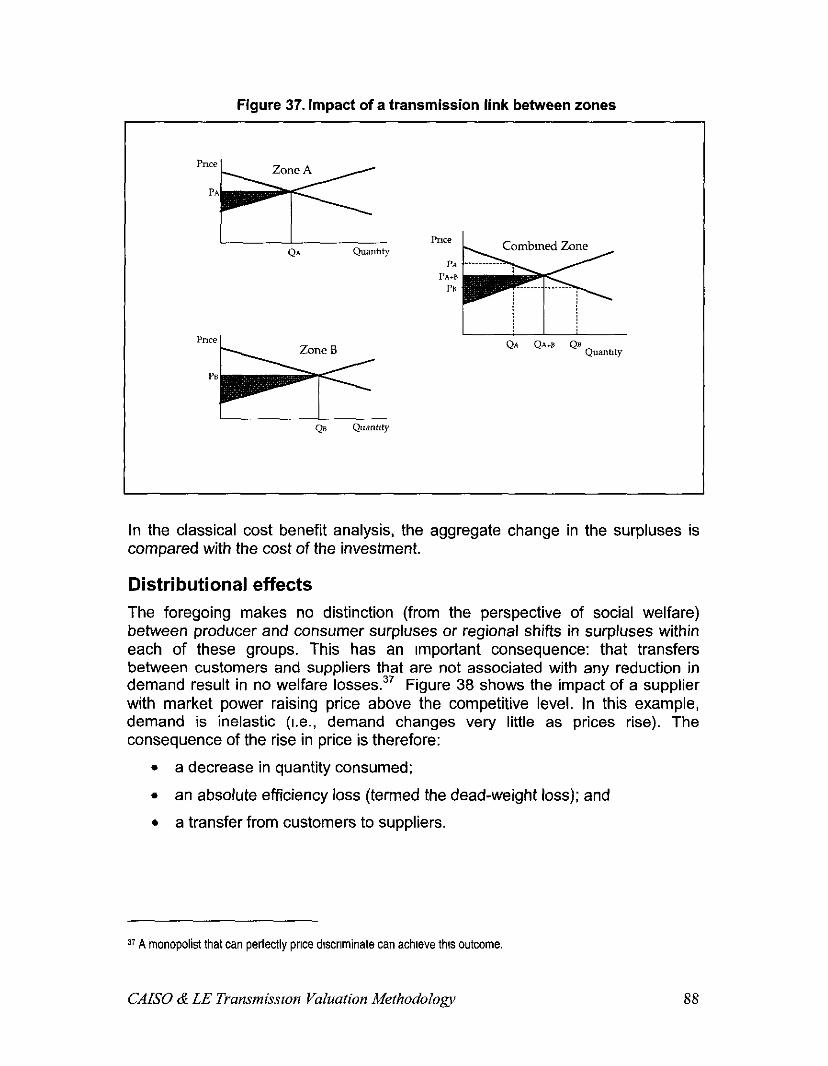
Figure 37. Impact of a transmission link between zones
In the classical cost benefit analysis, the aggregate change in the surpluses is compared with the cost of the investment.
Distributional effects The foregoing makes no distinction (from the perspective of social welfare) between producer and consumer surpluses or regional shifts in surpluses within each of these groups. This has an Important consequence: that transfers between customers and suppliers that are not associated with any reduction in demand result in no welfare losses.37 Figure 38 shows the impact of a supplier with market power raising price above the competitive level. In this example, demand is inelastic (I.e., demand changes very little as prices rise). The consequence of the rise in price is therefore:
l a decrease in quantity consumed;
l an absolute efficiency loss (termed the dead-weight loss); and
l a transfer from customers to suppliers.
37 A monopolist that can perfectly price dlscrlminate can achwe this outcome.
CAlSO & LE Tmnsmissron Valuation Methodology 88
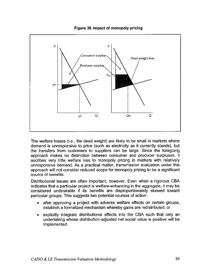
Figure 38. Impact of monopoly pricing
Consumer surplus I: bead weight loss
I
The welfare losses (i.e., the dead weight) are likely to be small in markets where demand is unresponsive to price (such as electricity as it currently stands), but the transfers from customers to suppliers can be large. Since the foregolng approach makes no distinction between consumer and producer surpluses, It ascribes very little welfare loss to monopoly pricing in markets with relatively unresponsive demand. As a practical matter, transmission evaluation under this approach will not consider reduced scope for monopoly pricing to be a significant source of benefits.
Distributlonal issues are often important, however. Even when a rigorous CBA indicates that a particular project is welfare-enhancing in the aggregate, it may be considered undesirable If its benefits are disproportionately skewed toward particular groups. This suggests two potential courses of action:
. after approving a project with adverse welfare effects on certain groups, establish a formalized mechanism whereby gains are redistributed; or
l explicitly integrate distributional effects into the CBA such that only an undertaking whose distribution-adjusted net social value is positive will be implemented.
CAB0 & LE Transmission Valuation Methodology 89
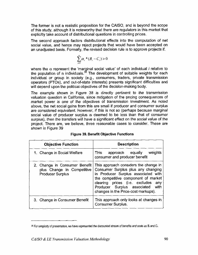
The former is not a realistic proposition for the CAISO, and is beyond the scope of this study, although it is noteworthy that there are regulators in this market that explicitly take account of distributional questions in controlling prices.
The second approach factors distributional effects into the computation of net social value, and hence may reject projects that would have been accepted on an unadjusted basis. Formally, the revised decision rule IS to approve projects if.
where the CL represent the ‘mar the population of n individuals. 8
inal social value’ of each individual i relative to The development of suitable weights for each
individual or group in society (e.g., consumers, traders, private transmission operators (PTOs), and out-of-state interests) presents significant difficulties and will depend upon the political objectives of the decision-making body.
The example shown in Figure 38 is directly pertinent to the transmission valuation question in California, since mrtigatron of the pricing consequences of market power is one of the objectives of transmission investment. As noted above, the net social gains from this are small if producer and consumer surplus are considered equivalent. However, if this is not so (perhaps because marginal social value of producer surplus IS deemed to be less than that of consumer surplus), then the transfers will have a significant effect on the social value of the project. There are, we believe, three reasonable cases to consider. These are shown in Figure 39
Figure 39. Benefit Objective Functions
Objective Function
I. Change in Social Welfare
2. Change in Consumer Benefit plus Change in Competitive Producer Surplus
3. Change in Consumer Benefit
Description
This approach equally weights consumer and producer benefit
This approach considers the change in Consumer Surplus plus any changing in Producer Surplus associated with the competitive component of market clearing prices (i e. excludes any Producer Surplus associated with changes in the Price-cost markups).
This approach only looks at changes in Consumer Surplus.
38 For slmpfuty of presentation, we have represented the dwounted stream of benefits and costs as B, and Cl.
CAB0 & LE Transmission Valuation Methodology 90

The first might be considered more consistent with a fully deregulated market where there is considerable customer choice and competition. The second might be considered more consistent with a market in which a regulator of final prices has an objective to ensure ongoing supply to customers at lowest sustainable price. Under this measure, no marginal social value is ascribed to positrve economic profits by generators derived from strategic bidding behavior (i.e. market power). The third approach focuses exclusively on consumer surplus with no consideration for producer surplus, Since competitive producer surplus (Le. producer surplus devoid of market power rents) is not apt to change much under most transmission expansions due to the homogeneity of thermal production costs throughout the western interconnect, there may not be much discernable difference between the second and third approach.
Since different agents can take drfferent views of the marginal social value of different surpluses, the most useful output from the transmission valuation methodology will be the buildrng blocks necessary to evaluate the given transmission investment project under all three drfferent objective functions. Appendix C provides a detailed methodology for how to estimate each of these benefits.
CAB0 & LE Transmission Valuation Methodology 91

Measuring Costs As noted above measuring the Net-Present Value of a transmission project can be expressed mathematically as:
NPV = B, -co B, -c, 4 -C, (l+d)O +(l+d)] +-+(l+d)’
>o
where the subscripts represent periods from project initiation, d embodies a social discount rate and B and C represent benefits and costs respectively. The annual costs of a transmission project should reflect the estimated annual revenue that a transmrssion owner would require to undertake the project Besides the capital costs of a project, these costs typically include a return on capital, federal and state taxes, and operation and maintenance costs (O&M). If no detailed cost estimates of these additional components are available at the time the project is being evaluated, they could be estimated using general utility standard (e.g. previously approved rates or return on equity and debt for previous projects and estimated taxes and O&M).
For the Illustrative Path 26 analysis, only the estimated capital cost of the proposed expansion was available. These are shown below In Figure 40 below. The exposed expansion consists of a short-term upgrade of 400 MW and two potential long-term upgrade options that would add an additional 600 MW of capacity in both directions. Option 1 was assumed as the long-term expansion option in the illustrative Path 26 analysis.
Figure 40. Path 26 Expansion Capital Costs
Capital
Upgrade
On-line Dates
Short-term
$2,100,000
400 MW
2003
Long-term
Option 1 Option 2
$138,750,000 $143,000,000
600 MW 600 MW
2005 2005
Social Discount Rate An important component of the NPV calculation is determining an appropriate social discount rate (d). There is no defimtive source or method for determining an appropriate socral discount rate. However, as a practical matter, regulators have already determined what they consider to be an appropriate rate of return on transmission assets, and have presumably taken into account all relevant considerations. Given this, the regulated rate of return approved for pervious transmission projects should serve as an appropriate discount rate. It should be noted that this rate may not necessarily correspond with the rate of return a
CAB0 & LE Transmrssion Valuation Methodology 92
transmission provider may be requesting to undertake a transmission project and it need not be. For example, an independent transmission company may offer to build a transmission expansion provided they can earn a 12% return on capital and the social dtscount rate, which is an average of the regulated rate of return of previously approved projects, may be 9%. In such a case, the 12% return will be reflected in the annual revenue requirements (C,) but the social discount rate will be 9%. In other words, the social discount rate should reflect the societal opportunity cost of money not the transmission investors.
It is important to note that if the benefits of a transmission expansion are adjusted for inflation (i.e. expressed in real dollars versus nominal dollars) then the social discount rate should also be adjusted for inflation in order to reflect the tnflation- free results; such an adjustment could be made by companng the yield on long- term US Treasury Bonds with the yield on an Inflation-indexed Treasury security.
CAISO & LE Transmission Valuation Methodology 93
VII. Summary of Methodology This document provides a comprehensive methodology for evaluating the economic benefits of transmission expansions. Specifically, this study addressed the following elements:
. Provides guidelines for determining the appropriate level of network representation and modeling time horizon.
. Describes the critical input data to a transmission valuation methodology and provides recommendatrons on the factors one should consider in choosing the appropriate values of these data.
l Identifies the major modeling components that a comprehensive valuation methodology should include and provides specific methodologies for developing each of them.
. Emphasizes the importance of estimating the benefits of a transmission expansion under multiple scenarios and provides a methodologies for selecting scenarios and assigning weights to each scenario in order to estimate the expected benefits of the expansion.
. Provrdes an overview of the theory and methodology for measuring the net-benefits of a transmission expansion and provides recommendations for specific benefit measures and methodologies for calculating these benefits
A summary of this comprehensive approach is provided in Figure 41
CAISO & LE Transmission Valuation Methodology 94
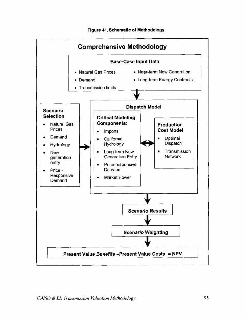
Figure 41. Schematic of Methodology
Comprehensive Methodology
Base-Case input Data
. Natural Gas Prices l Near-term New Generation
l Demand . Long-term Energy Contracts
. Transmission limits
Scenario Selection
. Natural Gas Prices
l Demand
. Hydrology
. New generation entry
. Price - Responsive Demand
.
Dispatch Model
1: ,w,w I
Scenario Results
Critical Modeling Components:
l Imports
l California Hydrology
l Long-term New Generatlon Entry
. Price-responsive Demand
l Market Power
Production Cost Model
l Optimal Dispatch
l Transmission Network
Scenario Weighting
Present Value Benefits -Present Value Costs = NPV
CAISO & LE Transmis.~ion Valuation Methodology 95
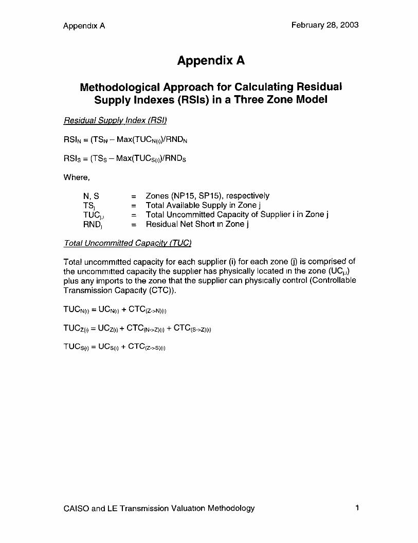
Appendrx A
Appendix A
February 28,2003
Methodological Approach for Calculating Residual Supply Indexes (RSls) in a Three Zone Model
Residual Supplv Index K3I)
RSIN = (TSa - Max(TUCa(,))/RNDN
RSls = (TSs - Max(TUCs(,))/RNDs
Where,
N, S = Zones (NP15, SP15), respectively TS, = Total Available Supply in Zone j WC,,, = Total Uncommitted Capacity of Supplier i in Zone j RND, = Residual Net Short In Zone j
Total Uncommitted Capacitv (TUG)
Total uncommrtted capacity for each supplier (i) for each zone (j) is comprised of the uncommrtted capacity the supplrer has physically located in the zone (UC,,,) plus any imports to the zone that the supplier can physically control (Controllable Transmission Capacity (CTC)).
TUCN(,) = UCN(,) + CTC(Z->N)(I)
TUCz(l) = UCz(t) + CTC(N.>Z)(~) + CTC(s->z)(t)
-WCs(,) = UCs(,) + CTC(z.>s)(,)
CAISO and LE Transmission Valuation Methodology 1
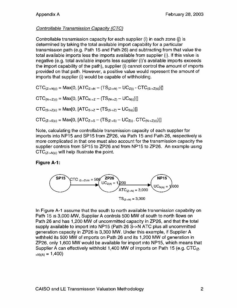
Appendix A February 28,2003
Controllable Transmission Capacitv (CTC)
Controllable transmission capacity for each supplier (i) in each zone (j) is determined by taking the total available import capability for a particular transmissron path (e.g. Path 15 and Path 26) and subtracting from that value the total available imports less the imports available from supplier (I). If this value is negative (e.g. total available imports less supplier (i)‘s available imports exceeds the import capability of the path), supplier (i) cannot control the amount of rmports provided on that path. However, a positive value would represent the amount of imports that supplier (i) would be capable of withholding.
CTC(Z.>N)(I) = MaxP, [ATCZ.>N - (TS(Z.,N) - UCz(q - CTC(s-,z)(,))ll
CTC(N.>Z)(~) = MaxP, [AT&Z - (T~(N.>z) - UCN(JII
CTC(S.,Z)(,) = MaxP, WTCS.,Z - W(S.,Z) - UC~dll
CTC(Z->S)(~) = MaxIO, WTCz.>s - (TS(z.,s) - UCz(,) CTC(N->Z)(Q)II
Note, calculating the controllable transmission capacity of each supplrer for imports into NP15 and SP15 from ZP26, via Path 15 and Path 26, respectively IS more complicated in that one must also account for the transmission capacity the supplier controls from SP15 to ZP26 and from NP15 to ZP26. An example using CTC+N)(,) will help illustrate the point.
Figure A-l :
T+>N) = 3,300
In Figure A-l assume that the south to north available transmission capability on Path 15 IS 3,000 MW, Supplier A controls 500 MW of south to north flows on Path 26 and has 1,200 MW of uncommitted capacity in ZP26, and that the total supply available to import into NP15 (Path 26 S->N ATC plus all uncommitted generation capacity in ZP26 is 3,300 MW. Under this example, if Supplier A withheld its 500 MW of imports on Path 26 and its 1,200 MW of generation in ZP26, only 1,600 MW would be available for import into NP15, which means that Supplier A can effectively withhold 1,400 MW of imports on Path 15 (e.g. CT+ >N)(A) = 1,400)
CAISO and LE Transmission Valuation Methodology 2

Appendix B February 28,2003
Appendix B
Regional Cost Differences in Siting New Power Generation in California
This Appendix provides a summary and assessment of a draft report prepared for the CEC on the regional cost differences of siting new generation in California’. The analysrs in the report is divided into two phases. The report outlrned a 2-Phase research approach to assessing regional cost drfference that would include the costs associated with the following regional siting constrarnts.
Figure 6-l. New Generation Siting Cost Components
Phase 1 . Air quality offsets
T
l Water resources
. Biological resources
l Land use issues
. Infrastructure upgrades, such as transmission lines (230 and 500 kv), substatrons, natural gas pipelines, water lines, reclaimed water lines etc.
1
Phase 2 l Additional details on Phase 1 factors
l Efficiency and reliability (plant performance based on the meteorological conditions)
l Public involvement and controversy
l Envrronmental justice
l Noise
l Transportation and circulation
l Recreation
l Cultural resources
l Visual resources
. Environmental contamination.
However, the report only included cost rnformatron on the Phase l elements. For the purpose of the analysis, a base load combined cycle plant of size 500MW is considered for comparison. The plant has the following features.
3 Combined Cycle of nominal output of 500 MW S. Two Frame 7F technology Combustion Turbines (CTs) manufactured by
GE and one Steam Turbine (ST). = Each of these turbines has a nominal capacity of 175 MW each. ti The capital cost of construction is assumed to be in the range of $400 -
$500 Million. + All of the costs are in 2003 dollars.
1 This IS a draft report tttled “RegIonal Cost Differences- Siting New Power Generation In Callforma” prepared for the Callfornla Energy Commissron by Aspen Enwonmental Group, December 2002.
CAISO and LE Transmission Valuation Methodology 1
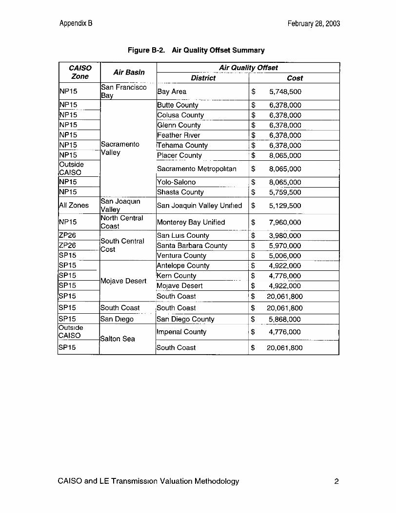
Appendix B February 28,2003
Figure B-2. Air Quality Offset Summary
CA/SO Air Basin Air Quality Offset
Zone District cost
NP15 San Francisco RX, Bay Area $ 5,748,500
ISP15 I /South Coast I $ 20.061 .a00
CAISO and LE Transmission Valuation Methodology

Appendix B February 28,2003
From Figure B-2 above the following costs are summarized for each of the CAISO zones.
Figure B-3. Air Quality Offset Summary by CAISO Zones
Figure B-4. Estimated Water Supply Costs and Capital Costs Associated with Cooling and Wastewater Discharge Systems
The costs shown in Figure B-4 are summarized for each of the CAISO zone in Figure B-5.
Figure B-5. Summary of Water Supply, Cooling System and Waste Water System cost
Cooling System Waste Water
CAISO and LE Transmission Valuation Methodology 3
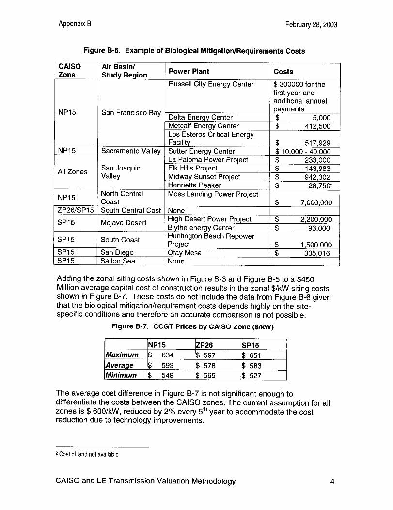
Appendtx B February 232003
Figure B-6. Example of Biological Mitigation/Requirements Costs
CAISO Zone
f
NP15
NP15
All Zones
NP15
ZP26lSP15
SP15
SP15 1-
SP15 SP15 t
Air Basin/ Study Region Power Plant
Russell City Energy Center
costs
$300000 forthe first year and additronal annual
San Francrsco Bay payments Delta Energy Center 5,000 Metcalf Energy Center i 412,500 Los Esteros Cntical Energy Facrlrty
.._ -..2 y Sutter Energy Center ; 10,000 “ZG La Paloma Power Project 233:000
Hills Project 143,983
Sacramento Vnlk
San Joaquin Vallev
Elk t Midwav Sunset Prornct - -, - - -
Henrietta Peaker i 28,750~ North Central Moss Landing Power Project Coast $ 7,000,000 South Central Cost None
Mojave Desert
South Coast
San Diego Salton Sea
High Desert Power Project $ 2,200,000 Blythe energy - I Center Huntington Beach Repower Project Otay Mesa None
$ 93,000
1,500,000 305,016
Adding the zonal siting costs shown in Figure B-3 and Figure B-5 to a $450 Million average capital cost of construction results in the zonal $/kW siting costs shown in Figure B-7. These costs do not include the data from Figure B-6 given that the biological mitigation/requirement costs depends hrghly on the srte- specific conditrons and therefore an accurate comparison IS not possible.
Figure B-7. CCGT Prices by CAISO Zone ($/kW)
ISP15 1 NP15 ZP26 Maximum $ 634 $ 597 $ 651
Average $ 593 $ 570 5 583 Minimum $ 549 $ 565 $ 527
The average cost difference in Figure B-7 is not significant enough to differentiate the costs between the CAISO zones. The current assumption for all zones is $6OO/kW, reduced by 2% every 5’h year to accommodate the cost reduction due to technology improvements.
2 Cost of land not available
CAISO and LE Transmission Valuatron Methodology 4
Appendix C February 28,2003
APPENDIX C
Defining Welfare Components and Transmission Benefits In the Transmission Evaluation Methodology
This Appendix describes the general approach used to calculate changes in consumer and producer welfare, and IS0 congestion charges. A simple two-zone example illustrates the approach. In Section I, we define the components of the welfare calculations without and with the transmissron addition. Then in Section II, we describe the calculation of welfare changes resultrng from the transmission expansion. Finally, in Section Ill, we discuss the modifications made to make the actual calculations using output of production costing simulation software.
I. Define Welfare Components
Without Transmission Expansion
Competitive Case
Figure C-l illustrates a snap shot of supply and demand balance in a 2-zone, l-way transmission system where Zone A is the importrng zone and Zone B is the exportrng zone, with a certain level of transmission capacity Tconnecting the two zones. Zone A IS short of generation, while B has a surplus of cheap generation. Suppose all generators bid their marginal costs and market clearing prices are settled at PO: and Pot where PO: > Pot due to congestron on the transmission line’. Line CA in the left panel represents the stack of the marginal costs of the generation units at A. The zonal demand in Zone A is represented by lrne @Bd\ where @ denotes the value of lost load in Zone A. Similarly in the right panel for the exporting zone, line \sFDa denotes the zonal demand curve where \/s denotes the value of lost load in Zone B, and line GE denotes the stack of the marginal costs of units located in Zone B. Note that there is excess supply of amount Tin Zone B; this represents exports to Zone A, which are used to meet the excess demand in Zone A.
’ Note the notation convention IS that superscrtpt “A” and “6’ denote zones, subscnpt “d’ denotes competltwe solution, and subscrlpt “~7 denotes solution In the absence of transmlsslon expansion
CAlSO & LE Transmission Valuation Methodology 1
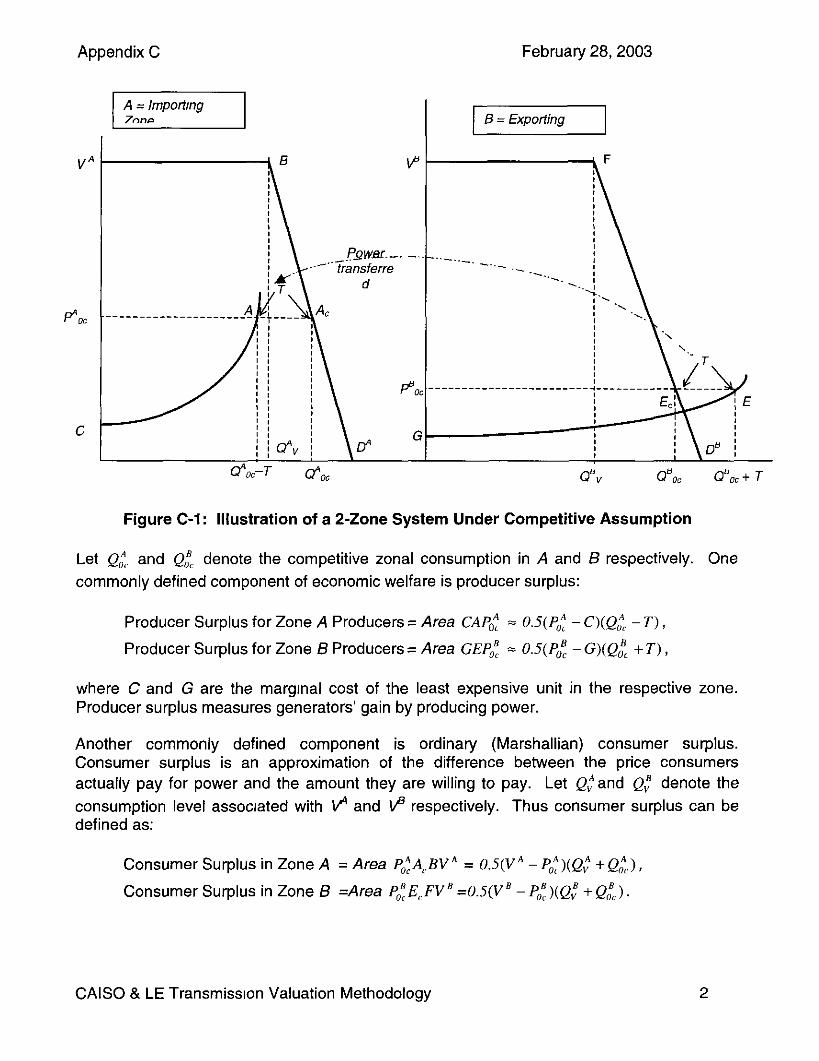
Appendix C February 28,2003
QdOC Q’oc + T
Figure C-l: Illustration of a 2-Zone System Under Competitive Assumption
Let Q,“, and Q,“, denote the competitive zonal consumption in A and B respectively. One commonly defined component of economic welfare is producer surplus:
Producer Surplus for Zone A Producers = Area CAP: = 0.5(Pk - C)(Q,“, -T) ,
Producer Surplus for Zone B Producers= Area GEPL = 0.5(PE -G)(QL +T),
where C and G are the margrnal cost of the least expensive unit in the respective zone. Producer surplus measures generators’ gain by producing power.
Another commonly defined component is ordinary (Marshallian) consumer surplus. Consumer surplus is an approximation of the difference between the price consumers actually pay for power and the amount they are willing to pay. Let Q;and Q,” denote the consumption level associated with p and 18 respectively. Thus consumer surplus can be defined as:
Consumer Surplus in Zone A = Area PLA,BVA = 0.5(VA - P’)(Q; +Qff,),
Consumer Surplus in Zone B =Area PLEcFVB =0.5(VB - PL)(Q,” + Q,“,)
CAISO & LE Transmissron Valuation Methodology 2
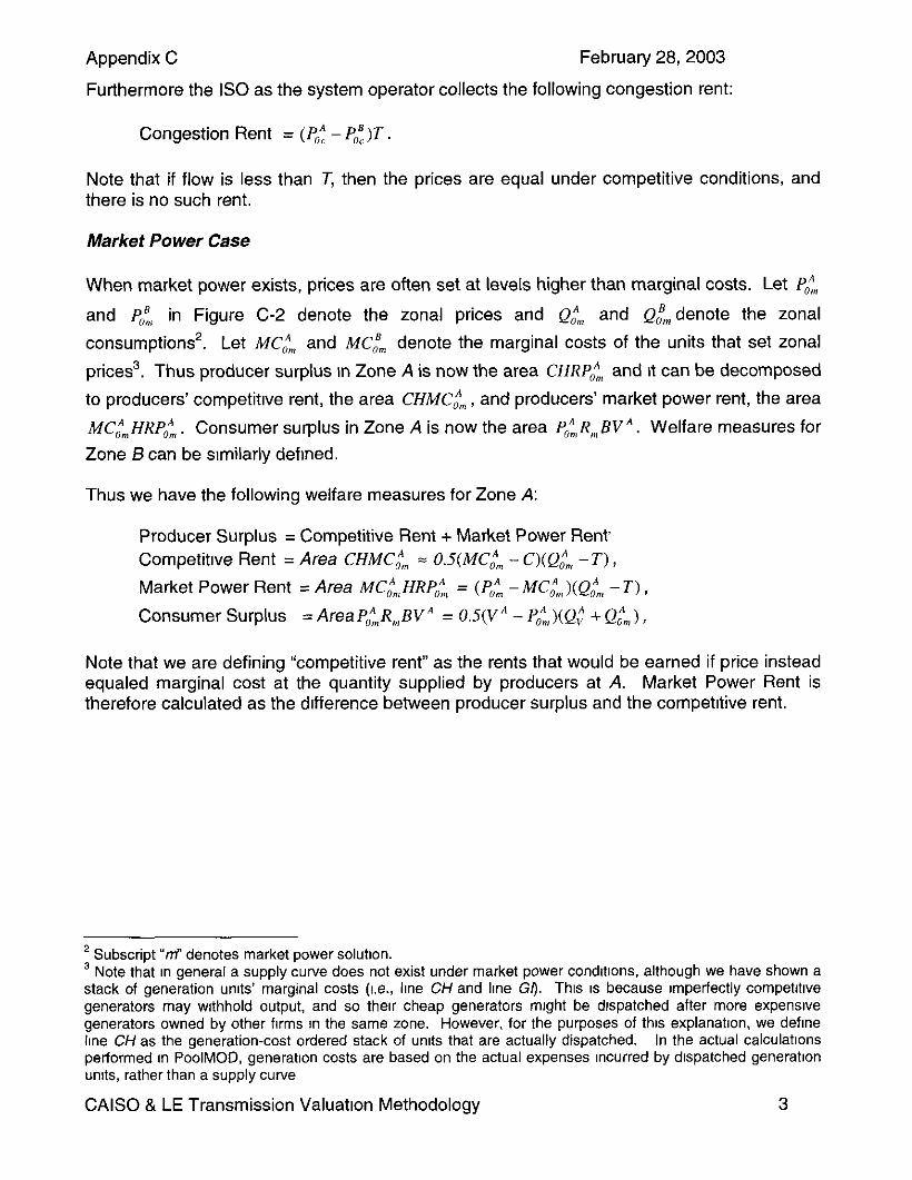
Appendix C February 28,2003
Furthermore the IS0 as the system operator collects the following congestion rent:
Congestion Rent = (Pz - PL)T
Note that if flow is less than T, then the prices are equal under competitive conditions, and there is no such rent.
Market Power Case
When market power exists, prices are often set at levels higher than marginal costs. Let Pim
and POi in Figure C-2 denote the zonal prices and Qim and Q,“, denote the zonal
consumption?. Let MC,4, and MC:“, denote the marginal costs of the units that set zonal
prices3. Thus producer surplus In Zone A is now the area CHRPA and It can be decomposed
to producers’ competitrve rent, the area CHIC,:, , and producers’ market power rent, the area
I!~C~~HRP~. Consumer surplus in Zone A is now the area Pk,R,,,BVA. Welfare measures for Zone B can be srmilarly defined.
Thus we have the following welfare measures for Zone A:
Producer Surplus = Competitive Rent + Market Power Rent Competitive Rent = Area CHMC& = 0.5(MCim - C)(Qi”, -T) ,
Market Power Rent = Area IVK$HRP& = (Pk - MC&)(Qtm -T) ,
Consumer Surplus =AreaPkR,BVA = 0.5(V” -Pk,)(Q{ +Qim).
Note that we are defining “competitive rent” as the rents that would be earned if price instead equaled marginal cost at the quantity supplied by producers at A. Market Power Rent is therefore calculated as the difference between producer surplus and the competitive rent.
’ Subscript “nf’ denotes market power solutron. 3 Note that rn general a supply curve does not exist under market power condrtrons, although we have shown a stack of generation unrts’ marginal costs (I.e., kne CH and lme Gf). Thus IS because rmperfectly competrtrve generators may withhold output, and so thetr cheap generators mrght be drspatched after more expensive generators owned by other firms rn the same zone. However, for the purposes of thus explanation, we define lrne CH as the generation-cost ordered stack of unrts that are actually dispatched. In the actual calculatrons performed rn PoolMOD, generatron costs are based on the actual expenses Incurred by drspatched generahon unrts, rather than a supply curve
CAISO & LE Transmission Valuation Methodology 3
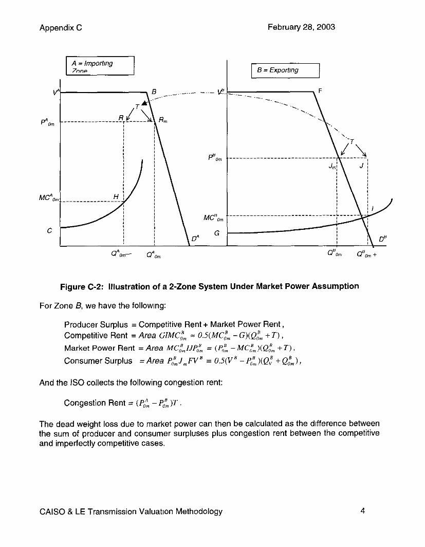
Appendix C February 28,2003
Figure C-2: Illustration of a 2-Zone System Under Market Power Assumption
For Zone B, we have the followlng:
Producer Surplus = Competitive Rent + Market Power Rent, Competitive Rent = Area GZMC,B, = O.S(MC,B, - G)(Q:“, + T) , Market Power Rent = Area MC~,IJP~ = (P,” - IWC:~)(Q:~ + T) ,
Consumer Surplus = Area P&lJ,FVB = 0.5(VB - Pk))(Q; + Q,“,),
And the IS0 collects the following congestion rent:
Congestion Rent = (PO”, - PA)T
The dead weight loss due to market power can then be calculated as the difference between the sum of producer and consumer surpluses plus congestion rent between the competitive and imperfectly competitive cases.
CAISO & LE Transmission Valuation Methodology
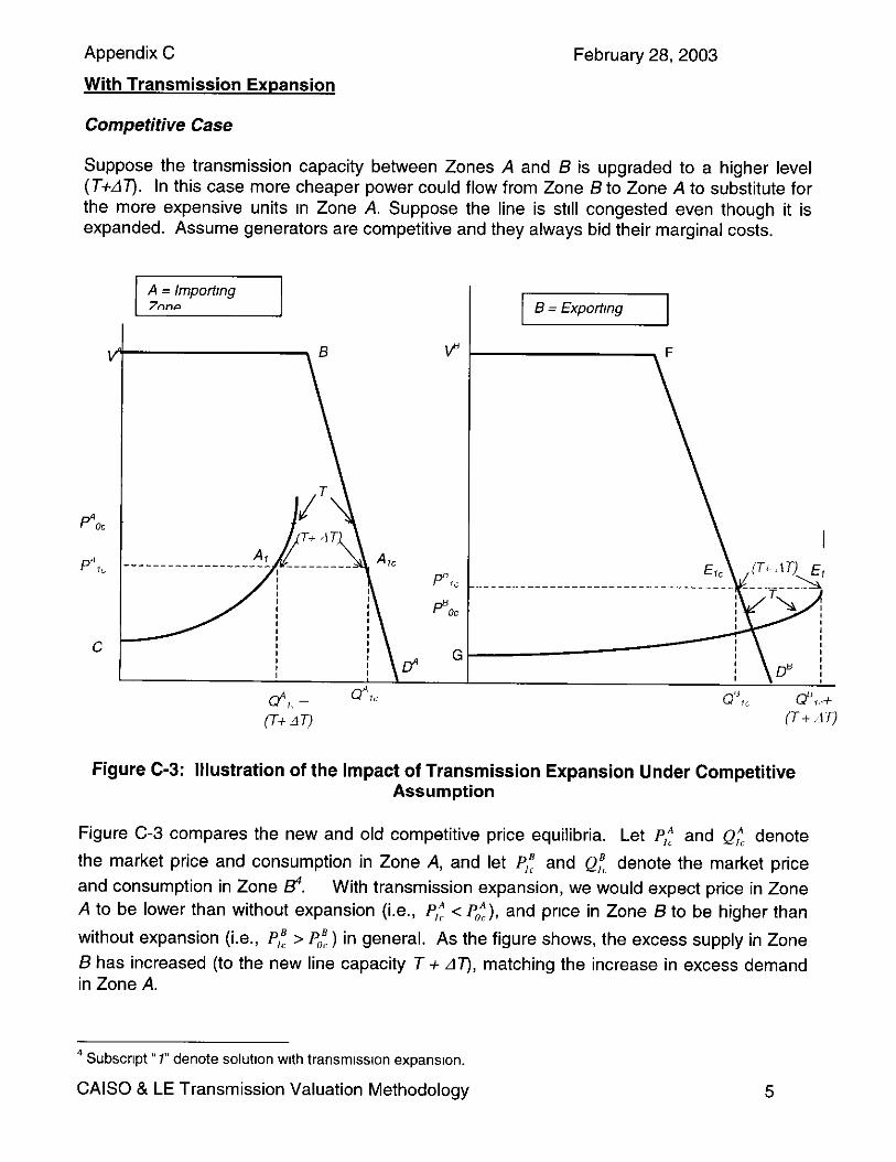
February 28,2003 Appendix C
With Transmission Expansion
Competitive Case
Suppose the transmission capacity between Zones A and 6 is upgraded to a higher level (T+AT). In this case more cheaper power could flow from Zone B to Zone A to substitute for the more expensive units In Zone A. Suppose the line is stall congested even though it is expanded. Assume generators are competitive and they always bid their marginal costs.
L a”,, - Q”a
(T+ AT)
1 B= Ex/mfmg 1
Q",, d';,d (T+ AT)
Figure C-3: Illustration of the Impact of Transmission Expansion Under Competitive Assumption
Figure C-3 compares the new and old competitive price equilibria. Let P,: and Qz denote
the market price and consumption in Zone A, and let P,: and Q,“, denote the market price and consumption in Zone @. With transmission expansion, we would expect price in Zone A to be lower than without expansion (i.e., P,: < PL), and price in Zone B to be higher than
without expansion (i.e., P,: > Pot) in general. As the figure shows, the excess supply in Zone B has increased (to the new line capacity T + AT), matching the increase in excess demand in Zone A.
a SubscrIpt ‘“7” denote solution with transmission expansion.
CAISO & LE Transmission Valuation Methodology 5

Appendix C February 28,2003
Under the competitive assumption, we have the following welfare measures:
Producer Surplus in Zone A = Area CA,P,: = O.S(P,: - C)[QL -(T + AT)],
Producer Surplus in Zone B = Area GE,P,f =OJ(P,f - G)[Qi + (T + AT)] ,
Consumer Surplus in Zone A = Area P,9A,‘BVA = 0.5(VA -P,:)(Q; +QL),
Consumer Surplus in Zone B =Area P,fE,p’ = 0.5(VB - P,f )(Q: + Q,“) ,
Congestion Rent = (P,: -P,f )(T + AT).
Market Power Case
When market power exists, prices are again set at levels higher than margrnal costs, although perhaps less so than before transmission capacity was expanded. Let P,“, and P,“,
denote the zonal prices and Q;“,, and Q,“, denote the zonal consumptions. Let MCtr and
MCf,denote the marginal costs of the units that set zonal prices in each zone respectively. Figure C-4 illustrates the resulting equilibrium, and calculations of welfare measures.
V
p”lm
p’,,,: L
- -. (T+ .<~I)
1 B=Export,ng 1
Q”,, (T+ LIT)
Figure C-4: Illustration of the Impact of Transmission Expansion Under Market Power Assumption
CAISO & LE Transmissron Valuation Methodology 6
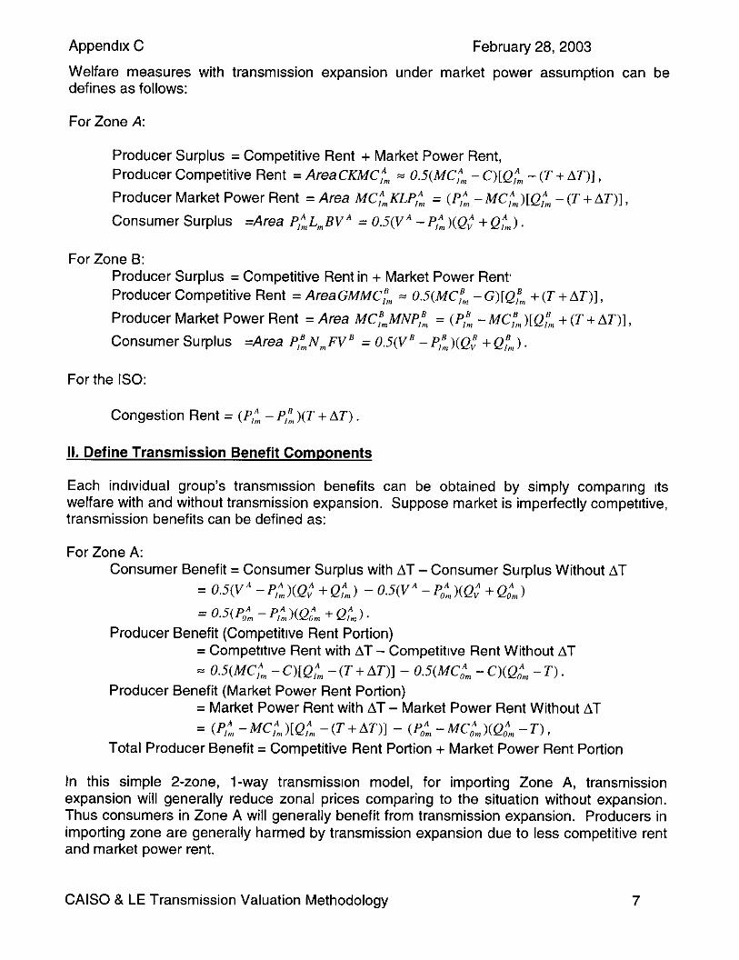
Appendix C February 28,2003
Welfare measures with transmrssion expansion under market power assumption can be defines as follows:
For Zone A:
Producer Surplus = Competitive Rent + Market Power Rent, Producer Competitive Rent = AreaCKMCfm = 0.5(MCfm - C)[Q,“, -(T + AT)],
Producer Market Power Rent = Area MCf,KLP,~ = (P,“, - MC~m)[Qfm -(T + AT)],
Consumer Surplus =Area P,~LmBVA = 0.5(VA -P,“,)(Q< +Qf”,).
For Zone B: Producer Surplus = Competitive Rent in + Market Power Rent Producer Competitive Rent = AreaGMMCfm = 0.5(MCfm - G)[Q,“, + (T + AT)],
Producer Market Power Rent = Area MCfmMNP,t = (P,fz - MCf,,)[Qfm + (T + AT)],
Consumer Surplus =Area P,“,N,FVB = 0.5(VB - P,ft)(Q: +Qi,).
For the ISO:
Congestion Rent = (P,“, - P,“,)(T + AT).
II. Define Transmission Benefit Components
Each individual group’s transmrssion benefits can be obtained by simply companng Its welfare with and without transmission expansion. Suppose market is imperfectly competrtive, transmission benefits can be defined as:
For Zone A: Consumer Benefit = Consumer Surplus with AT - Consumer Surplus Without AT
= 0.5(VA - P,“,)(Q,” + Q,“,) - 0.5(VA - PA)(Q; + Qin,)
= ‘WJ’R, - p,“, XQ;, + Q,“,) Producer Benefit (Competitrve Rent Portion)
= Competitive Rent with AT - Competitive Rent Without AT = 0.5(MC,A, - C)[Q,“, -(T + AT)] - 0.5(MC,A, - C)(Q,A, -T)
Producer Benefit (Market Power Rent Portion) = Market Power Rent with AT - Market Power Rent Without AT
= (p,tz -MC;‘,, NQ;‘, - CT + WI - V’; - MC;m ,(Q ,4. -T) , Total Producer Benefit = Competitive Rent Portion + Market Power Rent Portion
In this simple 2-zone, l-way transmission model, for importing Zone A, transmission expansion will generally reduce zonal prices comparing to the situation without expansion. Thus consumers in Zone A will generally benefit from transmission expansion. Producers in importing zone are generally harmed by transmission expansion due to less competitive rent and market power rent.
CAISO & LE Transmission Valuation Methodology 7
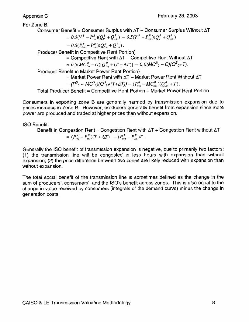
Appendrx C
For Zone B:
February 28,2003
Consumer Benefit = Consumer Surplus with AT - Consumer Surplus Without AT = 0.5(VB-P;)(Q; +QlB,) -OS(V'-P;)(Q; +Q,",, = 0.W'~ - PP,)tQ:,n + Q;,) .
Producer Benefit in Competitive Rent Portion) = Competitive Rent with AT - Competitive Rent Without AT zz O.S(MC,B, - G)[Q;, + (T + AT)] - 0.5(Mf?o - C)(@o+T,.
Producer Benefit In Market Power Rent Portion) = Market Power Rent with AT - Market Power Rent Without AT = (p,--MCf,)(@,+(T+AT))- (P," -MC,B,)(Q;nz +T).
Total Producer Benefit = Competitive Rent Portion + Market Power Rent Portion
Consumers in exporting zone B are generally harmed by transmissron expansion due to prices increase in Zone B. However, producers generally benefit from expansion since more power are produced and traded at higher prices than without expansion.
IS0 Benefit: Benefit in Congestion Rent = Congestion Rent with AT + Congestion Rent without AT
= (P,“, - P,f,)(T + AT) - (P, - P,,)T
Generally the IS0 benefit of transmission expansion IS negative, due to primarily two factors: (1) the transmission line will be congested in less hours with expansion than wrthout expansron; (2) the price difference between two zones are likely reduced with expansion than without expansion.
The total socral benefit of the transmission line IS sometimes defined as the change in the sum of producers’, consumers’, and the ISO’s benefit across zones. This is also equal to the change in value received by consumers (integrals of the demand curve) minus the change in generation costs.
CAISO & LE Transmission Valuation Methodology 8
Appendrx C
III. Calculation Method
February 28,2003
In the above we have defined welfare components and transmission benefits for a single time period of a 2-zone, l-way transmission system. Note in the real world, the import-export drrectron (thus net power flow direction) can be easily reversed depending on Instantaneous supply and demand balance in each zone and the transfer capability in both directions between zones. Thus ideally for long-term transmission expansion modeling, we should model a transmission network hourly or half-hourly and calculate welfare components and transmission benefits based on hourly or half-hourly market outputs, then aggregate to monthly or annual level to obtain transmission benefit for a given long-term time horizon.
Most production cost models can simulate hourly or half-hourly supply-demand balances, so does PoolMod. However, calculating welfare components by hourly or half-hourly intervals then aggregate IS very time consuming. An alternative approach is to use the quantity weighted average annual market prices and average generation costs with and without expansion to calculate annual welfares and benefits, We have experimented both approached and found out the second approach could generate reasonably good approximation for long-term transmission evaluation purposes.
CAISO & LE Transmission Valuation Methodology