513

A Buyer's Guide to Conic Fitting*

Andrew W. FitzgibbonRobert B. Fisher

Department of Artificial Intelligence, Edinburgh University5 Forrest Hill, Edinburgh EH1 2QL

Abstract

In this paper we evaluate several methods of fitting data to conic sec-tions. Conic fitting is a commonly required task in machine vision, butmany algorithms perform badly on incomplete or noisy data. We evalu-ate several algorithms under various noise and degeneracy conditions,identify the key parameters which affect sensitivity, and present theresults of comparative experiments which emphasize the algorithms'behaviours under common examples of degenerate data. In addition,complexity analyses in terms of flop counts are provided in order tofurther inform the choice of algorithm for a specific application.

1 Introduction

Vision applications often require the extraction of conic sections from image data.Common examples are the calculation of geometric invariants [2] and estimationof the centers and radii of circles for industrial inspection.

Many textbooks [5, 10] provide discussions and algorithms for least-squaresapproximation of conies, but these often include only the simple and fast algebraicdistance algorithm (algorithm LIN below). This algorithm fares poorly on manyreal data sets due to its inherent statistical bias, particularly when the image curvesare partially occluded. A number of authors [1, 6, 8, 9, 12, 13] have proposedalternative algorithms and while these are usually compared by the authors withLIN, there have been, to our knowledge, no comparative studies of the relativeaccuracy and efficiency of these alternatives.

This paper makes two important contributions to this area of computer visionresearch:

• Identification of the main conditions under which the algorithms fail. Itis common for comparative evaluations to concentrate on noise sensitivity,but in the case of conic fitting the important parameter is the amount ofocclusion.

• Presentation of the algorithm complexities in terms of flop counts allowsevaluation of the tradeoff between accuracy and speed of execution withoutreference to the specifics of an implementation and environment.

•This work was funded by UK EPSRC Grant GR/H/86905.

BMVC 1995 doi:10.5244/C.9.51

514

The four methods compared differ primarily in terms of the error measure thatthey minimize and then in terms of the techniques that are used to minimize thismeasure. In particular, the error measure determines the eventual accuracy of themethods and generally dictates the choice of optimization algorithm and hencetheir execution speed.

2 Problem Statement

The problem which the algorithms presented in this paper solve may be stated asfollows. Given:

• A set of 2D data points P — {x,}"=1, where x; = (a;,-, $/,•);

• A family of curves C(a) parameterized by the vector a;

• A distance metric 8(C'(a), x), which measures the distance from a point x tothe curve C(a);

find the value am;n for which the error function £2(a) = £]™_i (5(C(a),Xj) attainsits global minimum. The curve C(a) is then the curve that best fits the data.

In this paper, the curve families considered are represented in the implicit formC(a) = {x | F(a;x) — 0}. The two families that we examine are general conicsections, with F(a;x) = Axxx

2 + Axyxy + Ayyy2 + Axx + Ayy + AQ\ and circles,

for which Fc(a;x) = Ar(x2 + y2) + Axx + Ayy + Ao.

Finally we note that these forms may be written in a way that separates theparameters Aa from the terms in x using the dot product

F(a;xj) = [x2 x{y{ y2 xt yt 1] • [Axx Axy Ayy Ax Ay Ao]

= Xi -a

3 The Algorithms

3.1 Algorithm LIN: Algebraic Distance

The algebraic distance algorithm minimizes the objective function

subject to the constraint that ||a||2 = 1. The design matrix D is the n x 6 matrixwith rows Xi- The constrained objective function E = ||-Da||2 — A(||a|| — 1) =&TDTDa.—A(aTa— 1) is minimized analytically to form an eigenvector problem [4]:

V a £ = 0 <̂ => 2DTDa - 2Aa = 0

where A is a Lagrange multiplier. The minimizer amjn is then the eigenvector ofDTD corresponding to the smallest eigenvalue.

515

The algorithm requires 12n multiplications and 14n adds (or approximately 26nflops1 for the construction of the 15 unique elements of DT D. Evaluation of theeigensystem by Hessenberg reduction and QR generally took about 20 iterations(1700 flops) in our experiments, giving a total complexity of about 26n + 1700flops.

3.2 Algorithm BOOK: Algebraic distance with quadraticconstraint

Bookstein's algorithm [1] attempts to reduce the bias of LIN by imposing a differentconstraint on the parameter vector a. He derives the constraint 1A\X + A2

xy +2Ayy — 1 and shows how this leads to the system

DTDa = A Aa

where A = diag(2,1, 2, 0, 0, 0). This is a rank-deficient generalized eigensystem,which Bookstein solves by block-decomposition.

BOOK requires the 26n flops of LIN to form the DT D matrix. The matrixinversion and eigensystem solution's mean flop count was 1165, yielding a totalcomplexity of 26n +1165 flops.

3.3 Algorithm AMS: "Approximate Mean Square"Distance

The "approximate mean square distance" metric, introduced by Taubin[13], min-imizes the unusual objective function

\ / v ~ * n 11 T—7 T - I / _ \ I I 9 II r"l _ 119 \ II r\ ri~9~

where the matrices Dx and Dy are the partial derivatives of D with respectto x and y. Restating the problem as the minimization of ||-Da||2 subject to||A;a||2 + | | A y a | | 2 = l , the minimizer amjn is then the eigenvector of the general-ized eigensystem [4]

DTDa = \(DTX Dx + DT

y Dy)a

corresponding to the largest eigenvalue.AMS requires the 26rt flops of LIN to form the DTD matrix, but negligible

additional time to form £)JDx + Dy"Dy from the elements of D. The generalizedeigensystem routine's mean flop count was 9700, yielding a total complexity of26n + 9700 flops.

'MATLAB [7] defines addition and multiplication to each contribute one flop, while Goluband van Loan [4] consider one flop to consist of a multiply-accumulate. The MATLAB definitioncorresponds more closely to the computer used to perform the experiments, on which bothmultiplication and addition require one clock cycle.

516

3.4 Algorithm GEOM: Geometric Distance

The geometric distance metric measures the orthogonal distance from the pointx to the conic section. This metric, proposed by Nakagawa and Rosenfeld [8], isapproximately unbiased if the errors in the data points are distributed normallyto the curve. The distance is evaluated at a point x by solving the simultaneousequations

p + AVF(a;p) = x

F(a;p) = 0

for p and defining <J(C(a),x) = ||x - p||2. These equations involve the solution ofa quartic equation, and while closed-form solutions exist, numerical instability canresult from the application of the analytic formula [10]. In our implementationwe extract roots from the eigensystem of the companion matrix [4]. This in turnmeans that analytic derivatives of S, and consequently Vat2(a), are difficult tocalculate.

Each evaluation of e2(a) involves the solution of n such quartics, averaging1300n flops per iteration for the eigenvalue calculation. The number of iterationsdepends on the minimization algorithm chosen, but it is clear that even with only10 iterations, GEOM is 3 to 4 orders of magnitude slower than the previous twoalgorithms, and therefore was not extensively tested in our experiments.

3.5 Algorithm BIAS: "Statistical" Distance

Another approach, proposed by Kanatani [6] and Porrill [9], improves the LINalgorithm by explicitly calculating its inherent statistical bias and subtracting thebias from the result of minimization. Because the calculation of the bias dependson knowing both the true minimum and the noise level, the process is iterateduntil the predicted bias results in a noise-level correction of zero. Kanatani callsthis metric the "statistical distance", and argues that its bias sensitivity is in factsuperior to the geometric distance in the case where the errors on the data pointsare spherically distributed. Due to pressure of space this paper discusses onlyKanatani's bias correction algorithm. A description of algorithm itself would betoo long to include here, due to its dependence on tensor arithmetic. Note howeverthat the published noise-level update formula [6, eq 21] should be replaced by

C +tr(Q)tr(MQ) + 2tr(MQ2

Complexity of the algorithm is of the order of 50n + 1000 flops per iteration, withour test runs taking an average of 10 iterations.

3.6 Algorithm B2AC: Algebraic distance with quadraticconstraint

The B2AC algorithm is ellipse-specific, imposing the constraint that A2xy—AAxxAyy

1. This cleverly converts the inequality A\y - 4AxxAyy > 0 into an equality by

517

0

-1

Medium Low

o- 1 0 1 - 1 0 1 -1 0 1

Figure 1: Visual depiction of the three noise levels used in the later experiments. TheHigh, Medium and Low levels correspond to standard deviations of 4, 1 and i pixelsrespectively.

incorporating the normalisation factor. The corresponding generalized eigensys-tem is not nonnegative definite, and is solved by the scheme of Gander [3]. B2ACrequires the 26n flops of LIN to form the DTD matrix. The matrix inversion andeigensystem solution's mean flop count was 5182.

4 Experiments

All experiments were conducted using the MATLAB system [7]. Eigensystems aresolved using the underlying EISPACK routines, while the derivative-free minimiza-tion needed for the GEOM algorithm used the Nelder-Mead simplex algorithm.Also, as the execution-speed characteristics of interpreted MATLAB programs arequalitatively different to those of equivalent programs in a compiled language, wegive no timing statistics other than the flop counts in the previous section.

Noise model

The noise model applied in all experiments is isotropic zero mean normally dis-tributed. Other models may also be considered, particularly a nonisotropic modelwhere the variance is perpendicular to the curve. However, as the experimentsillustrate, degree of occlusion of the curve rather than noise is the parameter towhich the algorithms are more sensitive.

Additionally, the noise model does not include any outlier component. This isbecause none of the described algorithms are statistically robust. The algorithmsmay be made robust in the usual ways [14], in which case an outlier componentwould be added. Qualitatively, the most important change that this might maketo the results presented here would be that timing considerations could prove lessunfavourable to the iterative algorithms than in the outlier-free case.

Experiments other than the first are performed with three 'typical' noise levels,depicted visually in Figure 1. The high, medium and low noise levels correspondroughly to standard deviations of 2, 1 and i pixels on an ellipse with a majordiameter of 20 pixels.

518

"5 1000c?

100

10

1

0.1

0.01Ia.£ 0.001o 0.25

Experiment 1: Center error vs. Noise level

o LINx AMS* BIAS+ BOOK• B2AO

0.5 16 32

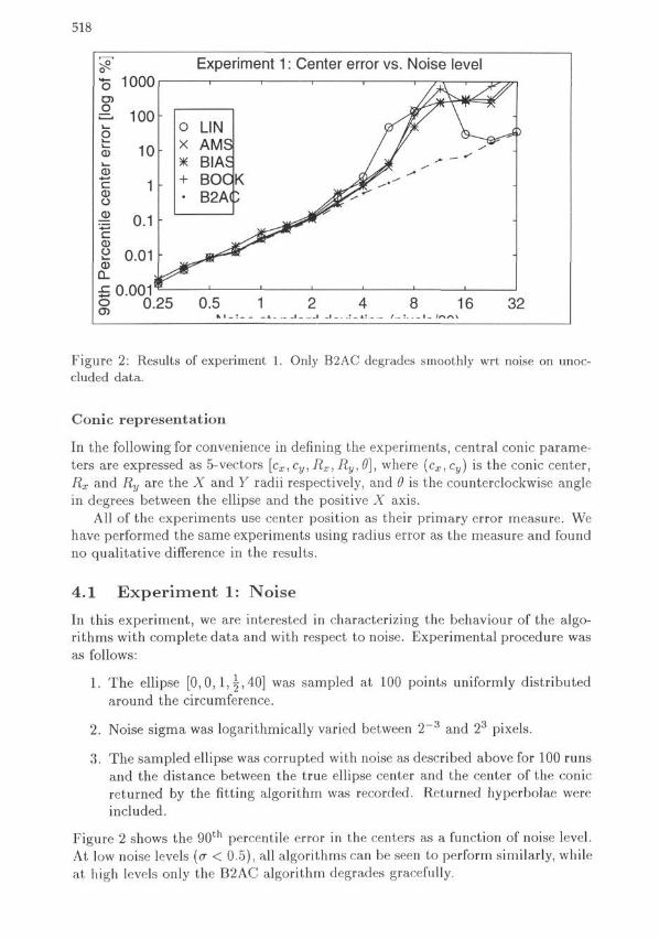
Figure 2: Results of experiment 1. Only B2AC degrades smoothly wrt noise on unoc-cluded data.

Conic representation

In the following for convenience in denning the experiments, central conic parame-ters are expressed as 5-vectors [cx, cy, Rx, Ry, 6], where (cx,cy) is the conic center,Rx and Ry are the X and Y radii respectively, and 6 is the counterclockwise anglein degrees between the ellipse and the positive X axis.

All of the experiments use center position as their primary error measure. Wehave performed the same experiments using radius error as the measure and foundno qualitative difference in the results.

4.1 Experiment 1: Noise

In this experiment, we are interested in characterizing the behaviour of the algo-rithms with complete data and with respect to noise. Experimental procedure wasas follows:

1. The ellipse [0,0,1,^,40] was sampled at 100 points uniformly distributedaround the circumference.

2. Noise sigma was logarithmically varied between 2~3 and 23 pixels.

3. The sampled ellipse was corrupted with noise as described above for 100 runsand the distance between the true ellipse center and the center of the conicreturned by the fitting algorithm was recorded. Returned hyperbolae wereincluded.

Figure 2 shows the 90th percentile error in the centers as a function of noise level.At low noise levels (a < 0.5), all algorithms can be seen to perform similarly, whileat high levels only the B2AC algorithm degrades gracefully.

519

Algorithm AMS Algorithm LIN Algorithm BOOKAIgorithm B2AC

0

-1-1 0

-11 -1

-11 -1

0

0-1

1 -1 0

25

S 15c§ 10CD

Experiment 2: Arc center error vs. Orientation

\\

\

/ N

:

LINAMSBIAS /

45 90 135 180 225 270Artrtla rxf nrr* ranlar

315 360

Figure 3: Results of experiment 2. Highest errors in center position occur at curvaturemaxima for LIN, between maxima and minima for AMS and BIAS.

4.2 Experiment 2: Orientation

In this experiment, we investigate how the errors in determining the center of a120° elliptical arc vary as the portion of the ellipse from which the arc is sampledrotates about the ellipse. This is so that in Experiment 3 we may ensure that thesubtended angle measurements are taken at the most pessimistic location aboutthe ellipse. Experimental procedure was as follows:

1. The counterclockwise orientation of the center of the arc was varied from 0to 360° in steps of 45°.

2. The ellipse [0,0,1,^,40] was sampled at 100 points uniformly distributedalong the 120° arc.

3. The sampled arc was corrupted with the three 'standard' noise levels asdescribed above.

4. The distance between the true ellipse center and the center returned by thefitting algorithm was recorded.

Figure 3 shows the results in two ways. The top three figures illustrate visuallythe located circle positions for algorithms AMS, LIN, BOOK and B2AC, while thebottom graph shows the error in median center position as a function of the arc

520

Experiment 3: NoiseLevefci

270 240 210 180 150 120Subtended Angle

Experiment 3: NoiseLevel=2

I 240 210 180 150 120 90 60 30 0Subtended Angle

Experimenl 3: NoiseLevetJ

240 210 1B0 150 120 90Subtended A note

Experiment 3: NotseLeveM Experiment 3: NoiseLevefcS Experiment 3: NoeeLeveW

270 240 210 180 150 120 90 60 30 0Subtended Angki

270 240 210 180 150 120 90 60 30 0Sifitanrtorl Annie

270 2 « 210 180 150 120SibtendtidAnde

Figure 4: Results of experiment 3. Results are for low, medium and high noise fromleft to right. The upper curves show the average sum of the errors in the principalpoints, while the lower ones show the proportion of non-ellipses produced by the conicalgorithms.

orientation. BIAS and AMS show their greatest errors at the 45° points, whilemaximum errors for LIN occur when the arc is sampled from the high curvaturesections at 0° and 180°.

4.3 Experiment 3: Occlusion

The third experiment is designed to locate the breakdown point of each of thealgorithms when the ellipse is progressively occluded. We measure the errors incenter position and radius estimates for several arcs of decreasing subtended angle.Experimental procedure was as follows:

1. The angle subtended by the elliptical arc was varied from 360° down to 0 insteps of 10°.

2. The ellipse [0,0,1, |,40°] was sampled at 100 points uniformly distributedalong the arc.

3. The sampled arc was corrupted with the three 'standard' noise levels asdescribed above.

4. Over 500 runs, the noisy arcs were submitted to each fitting algorithm. Thedistances of the fitted principal points to their correspondents on the true el-lipse were calculated. The mean sum distance where the algorithms returned

521

1

I0-8

| 0.6

a^0 .2

Experiment 4: Circle breakdown vs. subtended angle

o l_IN[Coriic)x AMSjfConic)* B2ACo — LINC:x — AMS

180 150 120 90

Figure 5: Results of experiment 4. The specialized circle fitters LINC and AMSC havebetter breakdown characteristics than the corresponding general conic algorithms.

ellipses was calculated, as was the percentage of runs in which non-ellipseconies were returned.

Figure 4 shows the plots of principal point error and percentage of returned non-ellipses as a function of decreasing subtended angle.

4.4 Experiment 4: Circles

In the final experiment, we consider the breakdown performance when the generalconic fitting algorithms are made specific to a particular task; in this case, circlefitting. Procedure is similar to Experiment 3, but we add two new algorithms,LINC and AMSC, which are specializations of LIN and AMS respectively. Figure 5shows the breakdown curves for the low-noise case. As expected, the specializedfitters LINC and AMSC break down considerably later than the general conicalgorithms.

5 Discussion

This paper has discussed the problem of fitting conic sections to ellipse data. Theexperiments illustrate that the key parameter affecting the algorithms' accuracyis the amount of occlusion present and the qualitative noise level. With completedata, all algorithms exhibit a similar degradation in the presence of increasingnoise.

As the data become progressively incomplete, a breakdown point is reachedbeyond which the algorithms fail catastrophically. This breakdown point is supe-rior with the B2AC and BIAS algorithms, and, in the special case of a circle, withthe circle-specific algorithms. Under high noise, BIAS has superior accuracy butproduces non-ellipses up to 60% of the time on highly occluded ellipses.

Algorithm complexities are, in increasing order: BOOK, LIN, B2AC, AMS,BIAS, GEOM.

522

Current and future work involves implementation and testing of the ellipse-specific algorithms of [11, 12], along with Porrill's alternative BIAS algorithm,and examining some alternative error metrics such as the conic invariants.

References

[1] F. Bookstein. Fitting conic sections to scattered data. Computer Graphicsand Image Processing, 9:56-71, 1979.

[2] D. Forsyth, J. L. Mundy, A. Zisserman, et al. Invariant descriptors for 3Dobject recognition and pose. IEEE T-PAMI, 13(10):971 991, 1991.

[3] W. Gander. Least squares with a quadratic constraint. Numerische Mathe-matik, 36:291-307, 1981.

[4] G. H. Golub and C. F. van Loan. Matrix Computations. Johns Hopkins, 2nd

edition, 1989.

[5] R. M. Haralick and L. G. Shapiro. Computer and Robot Vision, volume 1.Addison-Wesley, 1993.

[6] K. Kanatani. Statistical bias of conic fitting and renormalization. IEEET-PAMI, 16(3):320-326, 1994.

[7] The Math Works, Inc., Natick MA, USA. MATLAB Reference Guide, 1992.

[8] Y. Nakagawa and A. Rosenfeld. A note on polygonal and elliptical approxi-mation of mechanical parts. Pattern Recognition, 11:133-142, 1979.

[9] J. Porrill. Fitting ellipses and predicting confidence envelopes using a biascorrected kalman filter. Image and Vision Computing, 8(1):37—41, February1990.

[10] W. H. Press et al. Numerical Recipes. Cambridge University Press, 2ndedition, 1992.

[11] P. L. Rosin. Ellipse fitting by accumulating five-point fits. Pattern RecognitionLetters, 14:661-669, 1993.

[12] P. D. Sampson. Fitting conic sections to "very scattered" data. ComputerGraphics and Image Processing, 18:97-108, 1992.

[13] G. Taubin. Estimation of planar curves, surfaces and nonplanar space curvesdefined by implicit equations with applications to edge and range image seg-mentation. IEEE T-PAMI, 13(11):1115-1138, November 1991.

[14] P. Torr. Robust vision. In Proceedings, BMVC, 1993.