A Building Information Model (BIM) Based Lifecycle Assessment of a University Hospital Building Built to Passive House Standards

Blane Grann

Master in Industrial Ecology

Supervisor: Edgar Hertwich, EPT

Department of Energy and Process Engineering

Submission date: June 2012

Norwegian University of Science and Technology

i

Dedication I would like to dedicate this work to my parents for always encouraging me to pursue my interests and to Murielle for the sacrifices you’ve taken to make this happen.

ii

Preface This project was born out of a discussion I initiated with Geir Skaaren, part of the building operations staff at the Norwegian University of Science and Technology (NTNU), and my Supervisor Edgar Hertwich. My motivation was to establish a project that would be useful in helping the university improve the environmental performance of their building stock. While some initial pursuits of my own didn’t exactly pan out, it was established that the Kunskapssenter, a new, currently under construction university-hospital building in Trondheim, aiming to acheive passive house standards, would provide a unique case study for a whole building lifecycle assessment.

iii

Acknowledgements This thesis would not have been possible without the kind help of many people. Pål Ingdal at Helse Bygg Midt-Norge provided the data from the Building Information Model (BIM) that forms that basis of this analysis and assisted with my many inquisitions. Additional data for the energy model was provided by Marit Fjær (Cowi AS), and the demolition report by Wiggen Svein (Helsebygg-midtnorge). Edgar Hertwich provided the overall supervision of this work. Finally, I would like to thank all my fellow classmates in Industrial Ecology over the past two years that have made everything such a great experience.

iv

Abstract This thesis undertook a whole building lifecycle assessment of a university hospital building in Trondheim, Norway designed to passive house standards. The delivered energy for electricity and heating was estimated to be 122 kWh/m2. Impacts outside the energy used during the operational phase of the building were significant including 30% of greenhouse gas emissions, 41% of terrestrial acidification and 43% of particulate matter formation. Normalized to the number of staff, the building emits roughly 0.75 tonnes of CO2 equivalents per year over the 50 year life of the building.

v

Table of Contents Dedication ...................................................................................................................................................... i

Preface .......................................................................................................................................................... ii

Acknowledgements ...................................................................................................................................... iii

Abstract ........................................................................................................................................................ iv

Table of Contents .......................................................................................................................................... v

List of Figures ............................................................................................................................................. viii

List of Tables ................................................................................................................................................ ix

List of Acronyms ............................................................................................................................................ x

1 Introduction ........................................................................................................................................ 11

1.1 Motivation & Project Aim ........................................................................................................... 11

1.2 Lifecycle Assessment ................................................................................................................... 12

2 Literature Review ................................................................................................................................ 14

2.1 Previous Reviews ........................................................................................................................ 14

2.2 Review of Recent Contributions on Building LCA ....................................................................... 16

2.2.1 BIM ...................................................................................................................................... 16

2.2.2 Construction Phase ............................................................................................................. 16

2.2.3 Maintenance & Replacement ............................................................................................. 17

2.2.4 Building Operation: Energy Supply .................................................................................... 17

2.2.5 End of Life: Demolition and Waste Management .............................................................. 19

2.3 System Boundary ........................................................................................................................ 24

2.4 Summary ..................................................................................................................................... 24

3 Data & Methods .................................................................................................................................. 25

3.1 Case Description: Scope and System Boundary ......................................................................... 25

3.2 Data Sources ............................................................................................................................... 25

3.3 Lifecycle Inventory ...................................................................................................................... 27

3.3.1 Material Densities ............................................................................................................... 27

3.3.2 Transport Distances ............................................................................................................ 27

3.3.3 Maintenance and Replacement .......................................................................................... 28

3.3.4 Electricity Mix ...................................................................................................................... 29

3.3.5 District Heating System ....................................................................................................... 30

vi

3.3.6 Structural System ................................................................................................................ 31

3.3.7 Façade ................................................................................................................................. 32

3.3.8 Interior partitions ................................................................................................................ 37

3.3.9 Roof ..................................................................................................................................... 39

3.3.10 Balconies ............................................................................................................................. 41

3.3.11 Ceiling Coverings and Ceiling Walls .................................................................................... 41

3.3.12 Floor Coverings ................................................................................................................... 42

3.3.13 Interior wall Coverings ........................................................................................................ 42

3.3.14 Stairs .................................................................................................................................... 43

3.3.15 Construction ........................................................................................................................ 43

3.3.16 Demolition & Waste Management ..................................................................................... 43

5 Results and Analysis ............................................................................................................................ 46

5.1 Primary Energy Use ..................................................................................................................... 46

5.2 Advanced Contribution Analysis ................................................................................................. 47

5.2.1 Climate Change ................................................................................................................... 51

5.2.2 Human Toxicity ................................................................................................................... 51

5.2.3 Particulate Matter Formation ............................................................................................. 51

5.2.4 Terrestrial Acidification ....................................................................................................... 53

5.2.5 Freshwater Eutrophication ................................................................................................. 54

5.2.6 Freshwater Ecotoxicity ........................................................................................................ 54

5.2.7 Marine Ecotoxicity .............................................................................................................. 54

5.3 Sensitivity Analysis ...................................................................................................................... 55

6 Discussion ............................................................................................................................................ 58

7 Limitations and Future Work .............................................................................................................. 62

8 Conclusion ........................................................................................................................................... 64

Literature Cited ........................................................................................................................................... 65

Appendices .................................................................................................................................................. 75

Appendix A: Material Densities .............................................................................................................. 75

Appendix B: Transport Distances ........................................................................................................... 76

Appendix C: Architectural Drawings ...................................................................................................... 78

Appendix D: Demolition Report ............................................................................................................. 83

Appendix E: Process Summary ............................................................................................................... 85

vii

Appendix F: End-of-Life Processes ......................................................................................................... 97

Appendix G: Maintenance & Replacement .......................................................................................... 106

Appendix H: Tabular Results ................................................................................................................ 110

viii

List of Figures Figure 1: Global Urban/Rural Population Projections to 2050 .................................................................. 11 Figure 2: Energy Intensity for Building in Norwegian Service Industries 2008 .......................................... 11 Figure 3: Energy Intensity by US Commercial Building Type in 2008 ........................................................ 12 Figure 4: Lifecycle Energy Consumption in Residential Buildings .............................................................. 14 Figure 5: Lifecycle Energy Consumption of Office Buildings ...................................................................... 15 Figure 6: Marginal Emissions Factors for the Midwest (MRO), Texas (TRE), and Florida (FRCC) .............. 18 Figure 7: Waste Treatment in Norway ....................................................................................................... 19 Figure 8: System Boundaries for Building Material Disposal ..................................................................... 20 Figure 9: Ecoinvent v2.2 System Boundaries for Waste Disposal (W) and Energy Recovery (E) ............... 20 Figure 10: Open Loop Recycling – Same Primary Route ............................................................................ 21 Figure 11: Open Loop Recycling – Different Primary Route ...................................................................... 22 Figure 12: Life Cycle Carbon Emissions for a Multi-Story Wood Building Including End-of-Life Credits from Fossil Fuel Substitution ...................................................................................................................... 22 Figure 13: Relationship Between, Building, Bioenergy, and the Carbon Cycle .......................................... 23 Figure 14: System Boundary ...................................................................................................................... 26 Figure 15: European Flat Glass Producers in 2010..................................................................................... 28 Figure 16: Aluminum Mullion .................................................................................................................... 36 Figure 17: Cumulative Energy Demand Normalized by Total Heated Floor Area (17 354 m2) for a 50 Year Building Lifetime ......................................................................................................................................... 47 Figure 18: Advanced Contribution Analysis of Using ReCiPe, Midpoint, Hierarchist Method. Impacts Expressed per Unit Floor Area per Year for a 50 Year Building Lifetime .................................................... 49 Figure 19: Non-Electricity Lifecycle Emissions from Kunnskapssenter Normalized to A) Per Capita European Emissions, and B) Per Capita Global Emissions. ......................................................................... 50 Figure 20: Sensitivity Analysis – Relative change from Reference Scenario for Seven Impact Categories 56 Figure 21: Floor Area per Employee .......................................................................................................... 58 Figure 22: Carbon Footprint of NTNU ........................................................................................................ 59 Figure 23: Per Capita Emissions Budget for CO2 with and without Emissions Trading ............................. 60 Figure 24: Exterior Wall Details .................................................................................................................. 78 Figure 25: Composition of Interior Walls 1 ................................................................................................ 79 Figure 26: Composition of Interior Walls 2 ................................................................................................ 80 Figure 27: Technical Drawing – Main Building Roof .................................................................................. 81 Figure 28: Technical Drawing – Auditorium Roof ...................................................................................... 82

ix

List of Tables Table 1: Energy Consumption: End Use and Supply ................................................................................. 29 Table 2: NORDEL Electricity Mix ................................................................................................................. 30 Table 3: Trondheim District Heat Energy Supply Mix ................................................................................ 31 Table 4: Material Inventory – Structural System ....................................................................................... 32 Table 5: Mass Fraction of Steel in Reinforced Concrete Elements ............................................................ 32 Table 6: Material Inventory – Exterior Wall System .................................................................................. 33 Table 7: Material Inventory – Cladding ...................................................................................................... 34 Table 8; LCI – Curtain Wall ......................................................................................................................... 35 Table 9: Windows: Glazing Area and Window Frame Area in m2 ............................................................ 36 Table 10: Outer Door Types ....................................................................................................................... 37 Table 11: LCI – Interior Walls ..................................................................................................................... 37 Table 12: LCI – Interior Curtain Wall & Doors ............................................................................................ 38 Table 13: Material Composition of Interior Steel Doors ............................................................................ 39 Table 14: LCI – Roofing Systems ................................................................................................................. 40 Table 15: LCI – Balconies ............................................................................................................................ 41 Table 16: LCI – Ceiling Coverings and Walls ............................................................................................... 41 Table 17: LCI – Floor Coverings .................................................................................................................. 42 Table 18: LCI – Wall coverings .................................................................................................................... 42 Table 19: LCI – Stairs .................................................................................................................................. 43 Table 21: Non-Electricity Contributions to Climate Change ...................................................................... 51 Table 20: Non-Electricity Contributions to Human Toxicity....................................................................... 52 Table 22: Non-Electricity Contributions to Particulate Matter Formation ................................................ 52 Table 23: Non-Electricity Contributions to Terrestrial Acidification .......................................................... 53 Table 24: Non-Electricity Contributions to Freshwater Eutrophication .................................................... 53 Table 26: Non-Electricity Contributions to Freshwater Ecotoxicity ........................................................... 54 Table 25: Non-Electricity Contributions to Marine Ecotoxicity ................................................................. 55 Table 27: Parameters Assessed for Sensitivity Analysis ............................................................................. 55 Table 28: Primary Energy Use – Tabular Form ......................................................................................... 110 Table 29: Advanced Contribution Analysis – Tabular form...................................................................... 111

x

List of Acronyms BIM – Building Information Modelling

EIO-LCA – Economic Input Output Life Cycle Assessment

EPS – Expanded Polystyrene

XPS – Extruded Polystyrene

CED – Cumulative Energy Demand

11

1 Introduction It is widely understood that buildings

represent a key driver for global material and energy use. With the global urban population expected to roughly double between now and 2050 (see Figure 1), the building sector represents a priority area for cradle-to-grave environmental management. While the majority of new constructions will take place in developing and emerging markets due to mass rural-to-urban migration, innovations in the lifecycle performance of new buildings in developed countries will provide key lessons for the rest of the world to follow.

1.1 Motivation & Project Aim The literature on building lifecycle

assessments in dominated by multi-storey office buildings, single family residential dwellings, and multi-unit residential dwellings (Van Ooteghem & Xu, 2012). To my knowledge, no work has been done on hospital buildings which, per unit of floor area, are

amongst the most energy intensive building typologies (see Figure 2 for Norway and Figure 3 for the US).

The aim of this project is to undertake a whole building lifecycle assessment (LCA) of the Kunnskapssenter, a currently under construction University-Hospital building being located at St. Olav’s Hospital in Trondheim, Norway.

The innovative aspects of this LCA include: 1) a unique case study in a university-hospital building, 2) the low-energy, passive house objectives of the building, and 3) the use of Building Information Modeling for developing the life cycle inventory (LCI). Given the lack of identified

Figure 1: Global Urban/Rural Population Projections to 2050

Source: (United Nations, Department of Economic and Social Affairs, 2012)

Figure 2: Energy Intensity for Building in Norwegian Service Industries 2008

Source: Statistics Norway (2008)

0

1

2

3

4

5

6

7

Rural Urban Rural Urban

2011 2050

Billi

on P

erso

ns

12

literature pertaining to hospital buildings, the concern over problem shifting from the operation phase to other phases of the building life cycle, and the growth of BIM tools which have the potential to revolutionize how building LCAs are done, all three of these aspects provide an important contribution to the literature.

Recent requirements from Statsbygg (2007), the Norwegian government agency responsible for managing publicly owned buildings, has led to the use of 3D information modeling tools, Building Information Modeling (BIM), during the planning of new buildings to aid in the lifecycle management of buildings. Tools built into BIM software can be used to develop a life cycle inventory (LCI) for the material requirement of a building. In addition, the National Building Code in Norway (SINTEF Byggforsk, 2010a) requires energy assessments during the planning phase.

The main research questions answered in the thesis include:

1) What building systems make up the Kunnskapsenter? 2) What are the Lifecycle inventories of the building systems? 3) What is the lifecycle inventory of construction, maintenance and demolition activities? 4) How does the evaluation depend on assumptions regarding the emissions intensity of

the energy supply? Why is there disagreement about the intensity of supply?

1.2 Lifecycle Assessment Environmental LCA is a standardized method (ISO 2006) with methodology guidance provided

by organizations including the Institute for Environment and Sustainability, part of the European Commission Joint Research Centre (EU - JRC - IES 2010). The aim of lifecycle assessment is to provide a holistic framework for environmental assessment taking into account all phases of a product, service or system from the production of raw materials, to the manufacture, use and final disposal/recycling. The

Figure 3: Energy Intensity by US Commercial Building Type in 2008

Source: USDOE (2008)

0 100 200 300 400 500 600 700 800 900

kWh/

m2

Energy Intensity

Average

13

value of this perspective rests in identifying priority areas for intervention along the supply chain and can help address the issue of problem shifting. Reducing carbon emissions from the use stage, for example, of a product by increasing carbon emissions during the manufacturing stage can be quantified to assess the lifecycle changes in carbon emissions. The general methodology involves a three step process including: 1) identifying the scope and system boundaries for the assessment, 2) establishing the lifecycle inventory (LCI), and 3) completing the impact assessment. The scope refers to the system under investigation while, for practical reasons, the system boundaries establish the practical extent to which the system will be investigated. This is important for bottom-up process based LCA which requires detailed information for the LCI about specific materials, energy and waste at each stage of the lifecycle. Top-down, economic input-output LCA, on the other hand, applies cost data to economic input-output tables containing environmental stressors for economic sectors within an economy. All three stages of lifecycle assessment require a continuous, back-and-forth process of interpretation to ensure that the system boundaries are correct, that key processes are inventoried and that the results from the impact assessment provide a legitimate representation of the system under investigation.

14

2 Literature Review The aim of the literature review is twofold: first to present and discuss results reported in

recent literature reviews in the field of building LCA, and second, to review recent applications and key building LCAs to provide methodological insight and identify useful data sources to guide the LCA of the Kunnskapssenter. The first section more broadly discusses results and thematic output, while the second section delves into methodology and application.

2.1 Previous Reviews Previous review articles on building LCAs include: Sharma, Saxena, Sethi, Shree, & Varun (2011),

Ramesh, Prakash, & Shukla (2010), Optis & Wild (2010), Ortiz, Castells, & Sonnemann (2009) and Sartori & Hestnes (2007). These articles primarily address the topic of energy with the exception of Sharma et al. (2011), and Ortiz, Castells, & Sonnemann (2009). This section will briefly discuss the findings of these review articles.

Citing Adalberth, Almgren, & Petersen (2001), Sharma et al. (2011) report that 80-85% of lifecycle energy use occurs during the use phase of a building. As Gustavsson, Joelsson, & Sathre (2010) point out, it is not always clear when authors are referring to primary energy rather than the final energy delivered to the building which excludes transmission and distribution losses as well as efficiency losses in power plants. The lack of differentiation between primary energy and end-use energy is also present in the review by (Sharma et al., 2011).

Sharma et al. (2011) discuss the usefulness of Economic Input Output LCA (EIO-LCA) for quantifying energy and GHG emissions from the production of materials in the work of Norman, MacLean, & Kennedy (2006). EIO-LCA combines national financial tables broken down into different sectors of the economy with environmental stressor data for these sectors to get a top down view of emissions for each dollar of expenditure on a given sector. While less specific than process based LCAs, EIO-LCA can be helpful for getting an initial overview of the important materials or processes in a specific LCA which can then be used to target key materials using process LCA to improve the resolution (Joshi, 1999). The study by Norman, MacLean, & Kennedy (2006) found that brick, windows, drywall and

Figure 4: Lifecycle Energy Consumption in Residential Buildings

Source: Ramesh et al. (2010)

15

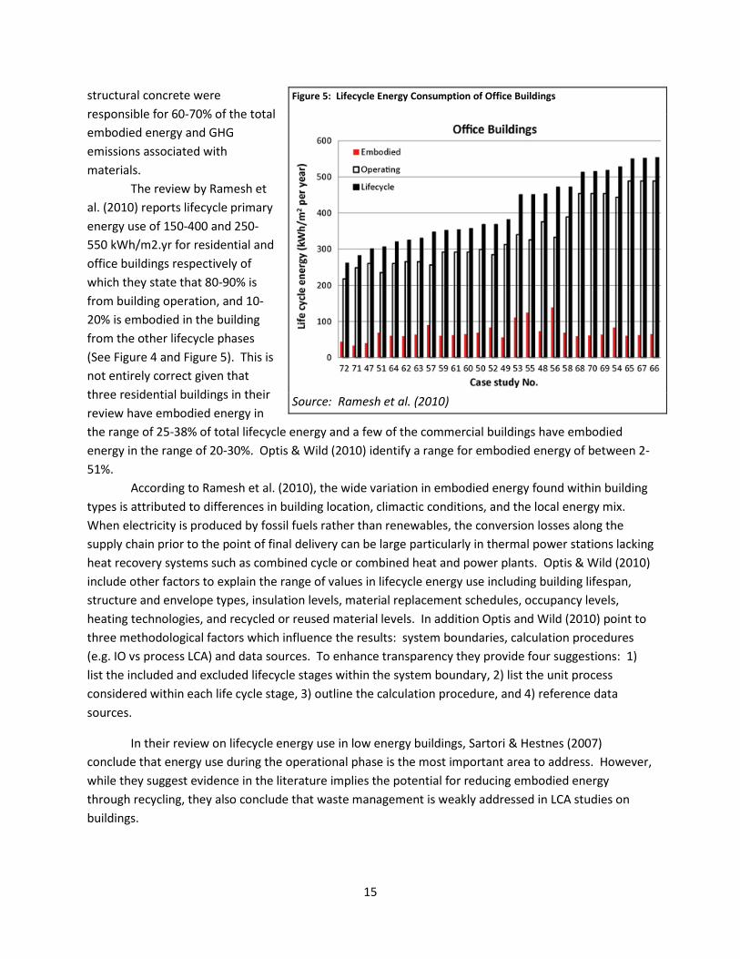
structural concrete were responsible for 60-70% of the total embodied energy and GHG emissions associated with materials. The review by Ramesh et al. (2010) reports lifecycle primary energy use of 150-400 and 250-550 kWh/m2.yr for residential and office buildings respectively of which they state that 80-90% is from building operation, and 10-20% is embodied in the building from the other lifecycle phases (See Figure 4 and Figure 5). This is not entirely correct given that three residential buildings in their review have embodied energy in the range of 25-38% of total lifecycle energy and a few of the commercial buildings have embodied energy in the range of 20-30%. Optis & Wild (2010) identify a range for embodied energy of between 2-51%.

According to Ramesh et al. (2010), the wide variation in embodied energy found within building types is attributed to differences in building location, climactic conditions, and the local energy mix. When electricity is produced by fossil fuels rather than renewables, the conversion losses along the supply chain prior to the point of final delivery can be large particularly in thermal power stations lacking heat recovery systems such as combined cycle or combined heat and power plants. Optis & Wild (2010) include other factors to explain the range of values in lifecycle energy use including building lifespan, structure and envelope types, insulation levels, material replacement schedules, occupancy levels, heating technologies, and recycled or reused material levels. In addition Optis and Wild (2010) point to three methodological factors which influence the results: system boundaries, calculation procedures (e.g. IO vs process LCA) and data sources. To enhance transparency they provide four suggestions: 1) list the included and excluded lifecycle stages within the system boundary, 2) list the unit process considered within each life cycle stage, 3) outline the calculation procedure, and 4) reference data sources.

In their review on lifecycle energy use in low energy buildings, Sartori & Hestnes (2007) conclude that energy use during the operational phase is the most important area to address. However, while they suggest evidence in the literature implies the potential for reducing embodied energy through recycling, they also conclude that waste management is weakly addressed in LCA studies on buildings.

Figure 5: Lifecycle Energy Consumption of Office Buildings

Source: Ramesh et al. (2010)

16

When considering low energy and energy self-sufficient homes, Ramesh et al. suggest that a limit exists for decreasing lifecycle energy use with the potential that “embodied energy will be so high that the total energy use during the life time will start to increase again” and therefore that “[t]oo many technical installations in order to make buildings self-sufficient are not desirable” (2010, p. 1598).

While these literature reviews have emphasized the dominant role of the operational phase of buildings for energy use and carbon emissions, a potential concern rests on the issue of problem shifting from the operational phase to other phases in the building life cycle. The investigation of a university-hospital building, typically very energy intensive buildings, that is built to passive house standards thus presents a unique opportunity to further consider this issue.

2.2 Review of Recent Contributions on Building LCA Turning to more recent contributions in the field of building LCA, the aim of this section is to

outline and discuss useful insights and challenges highlighted in recent building LCAs with a particular focus on commercial buildings.

2.2.1 BIM Of particular relevance to this thesis, Stadel et al. (2011) address the use of building information

modeling (BIM) and LCA in teaching sustainable building design. BIM is a tool for providing three-dimensional representations of buildings and building components. The dimension and volumes of building components (e.g. columns, doors, windows, etc.) by system type (e.g. building structure, façade, etc.) can be exported to excel for further analysis. According to Stadel et al. (2011), one of the main challenges in using BIM for LCA – in this case the BIM software was Autodesk Revit Architecture 2010 (Autodesk, 2012) – is that the material takeoff tool requires that composite materials be manually disaggregated in order to refine the individual material estimates. As an example, a reinforced concrete wall, or a wall with wooden studs, insulation and gypsum plaster board needs to be manually disaggregated into individual products.

2.2.2 Construction Phase Bilec, Ries, & Matthews (2010) suggest that the construction phase is often overlooked in

building LCAs. Their work applies a hybrid LCA methodology to the construction phase of a 6-story, steel framed commercial building focusing on the “major core and shell processes” (Bilec et al., 2010, p. 202). EIO-LCA was used for modelling services (e.g. architects, engineers, etc.), temporary material manufacture (such as form work), and the manufacture of construction equipment. Simarpro was used to model material transport, worker transport and electricity; the USEPA NONROAD2005 model was used for the energy combustion of non-road equipment. By comparing their results for the construction phase with results for a similar building structure from Guggemos and Horvath (2005), their results suggest that impacts during the construction phase are of the same order of magnitude as end of life and materials production.

Based on their literature review, Gustavsson et al. (2010) assume primary energy requirements for construction are 80 kWh/m2 for a multi-storey, wood framed apartment building – half electricity, and half diesel.

17

In an LCA of three common UK housing types, Cuéllar-Franca & Azapagic (2012) only consider energy use during the construction phase. The total construction energy requirement for each of the three residential buildings types in their assessment is based on the work of Adalberth (1997).

Williams, Elghali, Wheeler, & France (2011) adopt an IO approach for dealing with construction using national figures for the value of total construction and CO2 emissions.

According to ecoinvent documentation (Kellenberger et al., 2007), the building machines for excavation and demolition are the major diesel consumers. They estimate a requirement of 5MJ per m3 of above ground building and assume that 0.8 m3 of excavation is required for every 1.0 m3 of above ground building.

2.2.3 Maintenance & Replacement Cuéllar-Franca & Azapagic (2012) consider windows, doors and floor coverings for the

maintenance phase using replacement schedules from Anderson, Shiers, & Sinclair (2002). Iyer-Raniga & Wong (2012) use component lifetimes provided by the National Association of Home Builders in North America, while Williams et al. (2011) adopt component lifetimes from the life cycle costing book put out by the Building Cost Information Service (Royal Institute of Chartered Surveyors, 2006).

2.2.4 Building Operation: Energy Supply As noted above, the operational phase plays a significant role in the lifecycle energy consumption of a building. In this section the difference between attributional and consequential LCA is outlined and the relation between consequential modelling and the marginality principle in economics is introduced as a motivation for using consequential LCA principles to select the electricity mix used in LCA work. Allocation issues for energy production from municipal solid waste incineration, are discussed in the next section on waste management.

Given that energy use plays an important role in many environmental pressures, the electricity mix used in LCA work strongly influences the overall results. Unlike most goods, electricity has the unique property in which each electron is indistinguishable from the next meaning that it is not possible to track the consumption of electrons back to their source of origin in an interconnected grid. As electricity markets continue to become more integrated, the flow of electricity across borders and between markets continues to increase.

In methodological terms, attributional LCA takes a descriptive approach to model the system “as is” using a static technosphere and combining product specific data with average or generic data for products served by a market with many producers using different technologies (EC - JRC - IES 2010). But what then should one chose as an average electricity mix? Perhaps the scope of the analysis is set to the geographical borders of a country like Norway with the objective to minimize greenhouse gas emissions produced within Norway’s borders as outlined by the United Nations Framework Convention on Climate Change (Peters, 2008). Under the UNFCC agreement, GHG accounting is based on where the emissions are produced – the producer principle. 1 Aiming to reduce Norway’s domestically produced emissions thus imply using a Norwegian electricity mix to account for the actual emissions within Norway. 1 The producer principle is in contrast to the consumer principle in which emissions are allocated to the final consumers rather then the producer of the emissions. The choice allocation can be significant when considering the emissions embodied in international trade.

18

While an analysis using the Norwegian electricity mix would help identify important non-energy related GHG’s due to the low lifecycle emissions of the hydro power systems that provide the backbone of Norway’s electricity system, this ignores Norway’s electricity trade. In reality, we know that in an interconnected global marketplace, goods and energy flow across borders. Further, any low GHG emission electricity not consumed in Norway can potentially be exported to reduce high GHG coal and gas plants in other countries.

In contrast to the attributional approach described above, consequential LCA looks to grapple with some of these issues by modeling the specific consequences of, for example, a given reduction in electricity demand in Norway. In other words, consequential LCA models a dynamic technosphere (EU - JRC - IES 2010).

An excellent example of the use of consequential modeling of electricity is provided by Siler-Evans, Azevedo, & Morgan (2012). They develop marginal emissions factors (MEFs) for CO2, NOx, and SO2 in the US electricity market based on marginal generators in the system over various temporal horizons (see Figure 6). Their results demonstrate how using average emissions factors can misrepresent actual emissions within the system depending on the time of day, month, or year.

In economics consequential modelling has a long history under what is referred to as the marginality principle. Rather than the marginal emissions factors displayed in Figure 6, economists would be concerned with the marginal cost of producing electricity throughout the day, month or year which similarly depends on the marginal producing generator – the generator that is scaled up or down in response to a specific change in demand. Over a short time frame, this is referred to as the short-run marginal cost. When considering a longer time frame involving investment costs in new capacity, the assessment is referred to as the long-run marginal cost.

While an analysis of long-run marginal emissions factors using projected energy scenarios will be an important contribution to lifecycle modelling, such an analysis is well beyond the scope of this thesis. Instead, the analysis assumes a Nordic electricity mix grounded in the knowledge that “the cooperation with Norway and other Scandinavian countries is highly likely going to be necessary” for countries like Germany to achieve their renewable energy scenarios for 2050 (Lindberg, 2012 citing the German Advisory Council on the Environment). In short, reductions in the consumption of relatively clean Norwegian electricity within Norway can be exported to other European countries to displace higher emissions sources. In this respect, a Nordic electricity mix represents a conservative estimate of the

Figure 6: Marginal Emissions Factors for the Midwest (MRO), Texas (TRE), and Florida (FRCC)

Source: (Siler-Evans et al., 2012)

19

actual potential for reducing emissions in other markets. The purpose of assuming a Nordic electricity mix is thus to demonstrate the potential for reducing emissions in other markets through reducing Norwegian consumption.

2.2.5 End of Life: Demolition and Waste Management

Waste management includes the handling and treatment (i.e. recycling, reuse, incineration and land filling) of waste materials from the construction and demolition phases of the building. The aim of this section is to review relevant LCA literature for modelling waste management and discuss how the delineation of system boundaries can influence final results.

System boundaries are an important consideration in assessing waste management due to interactions with other system boundaries including energy systems and next-generation product lifecycles. With waste incineration and energy recovery playing an important role in Norwegian waste treatment (see Figure 7) allocation decisions used to distribute emissions between waste management and energy recovery has important implications for the results. After emphasizing the challenges associated with emissions allocation in waste incineration and energy recovery, the ecoinvent v2.2 report (Doka, 2009) on waste incineration outlines their rationale for allocating 100% of the emissions to waste treatment (a depiction of the system boundaries used for allocating emissions for waste incineration in ecoinvent v2.2 is provided in Figure 9). They argue that the principle function of the system is to treat waste rather than produce energy. Further they point out that an allocation based on economics would also heavily favour the side of waste management. The implication from allocating 100% of the emissions to waste treatment is obvious: the results provide little incentive for the energy consumer to reduce the ‘zero emission’ energy that they receive from garbage incineration while the entire burden is put on the waste treatment system which, as a side note, has little if any control over the drivers of waste production which rest in the hand of producers and higher levels of government.

Ecoinvent v2.2 (Doka, 2009) uses three system boundaries for end-of-life management of building materials: A) direct recycling, B) recycling after sorting, and C) disposal (see Figure 8). It is important to note that energy

Figure 7: Waste Treatment in Norway

20

use for demolition is always included in the system boundary while transport from the building site is only included for systems B and C.

Recycling presents another challenge with respect to allocation in LCA. Coelho & de Brito (2012) critique the assumption of Thromark (2002) in which the building waste products are integrated back into the building products chain without considering down-cycling. Cuéllar-Franca & Azapagic (2012)

Figure 8: System Boundaries for Building Material Disposal

Source: (Doka, 2009)

Figure 9: Ecoinvent v2.2 System Boundaries for Waste Disposal (W) and Energy Recovery (E)

Source: (Doka, 2009)

21

assume 100% virgin raw materials and instead credit the system for recycled and reused materials from end of life management. While the aim of Cuéllar-Franca & Azapagic (2012) is to avoid double counting by both crediting the system for using materials the contain a fraction of recycled material while also crediting the system for the substitution potential of next generation products – products that can avoid using virgin material by using recycled material from your system. Perhaps a better solution to assuming 100% virgin raw materials is to use an average material composition based on recycled and virgin sources as provided in a database like ecoinvent v2.2 while accounting separately for the potential benefits of substituting for raw materials in next generation products without crediting them to the system under study in the final results.

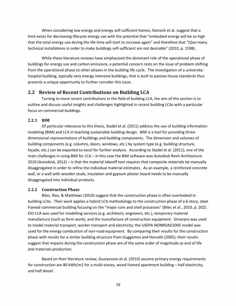
According to Paulik2, it is realistic to assume the reintegration of certain products into the building supply chain as depicted in Figure 11 such as the steel rebar used in reinforced concrete or the reinforcing steel in beams and columns. In Figure 11, assembly 1 and use 1 are functionally equivalent to assembly 2 and use 2 and the recycled material displaces primary materials. However, for aluminum products which are qualitatively understood to be recycled in a cascade in which building products represent the top of the hierarchy3, recycling is more properly modelled in what is referred to as ‘open loop – different primary route’ (see Figure 11) in which the recycled aluminum is used to replace primary aluminum that could be used, for example, in engine blocks which is dependent on a much smaller proportion of primary aluminum. The ILCD Handbook provides additional methodological guidance for lifecycle assessments of waste management (EC JRC IES 2010).

Coelho & de Britio (2012) outline a “top-down” process based LCA methodology for the construction and demolition waste management phase for buildings. The reference to top-down simply suggests that the data sources come from existing literature – primarily Blengini (2006) and Junnila (2004). The basis of their modeling requires allocating environmental impacts based on material

2 Paulik, S. (2012) personal communication 3 Liu, G. (2012) personal communication

Figure 10: Open Loop Recycling – Same Primary Route

Source: EC JRC IES (2010)

22

recycling and reuse rates described by five scenarios. The results from their analysis suggest that “[d]emolition/end-of-life environmental consequences are mainly conditioned by transportation” (Coelho & de Brito, 2012, p. 534). However, incineration is not a disposal route considered in any of their scenarios.

Coelho & de Brito (2012) point out that Blengini & Garbarino (2010) have given a thorough treatment of waste management in building LCA particularly with respect to concrete, aggregate, and steel. In their work, Blengini & Garbarino (2010) develop a model using GIS and LCA to evaluate the trade-offs between reduced emissions due to raw material substitution using recycled products, on the

Figure 11: Open Loop Recycling – Different Primary Route

Source: EC JRC IES (2010)

Figure 12: Life Cycle Carbon Emissions for a Multi-Story Wood Building Including End-of-Life Credits from Fossil Fuel Substitution

Source: (Gustavsson et al., 2010)

23

one hand, and greater transport related emissions on the other hand.

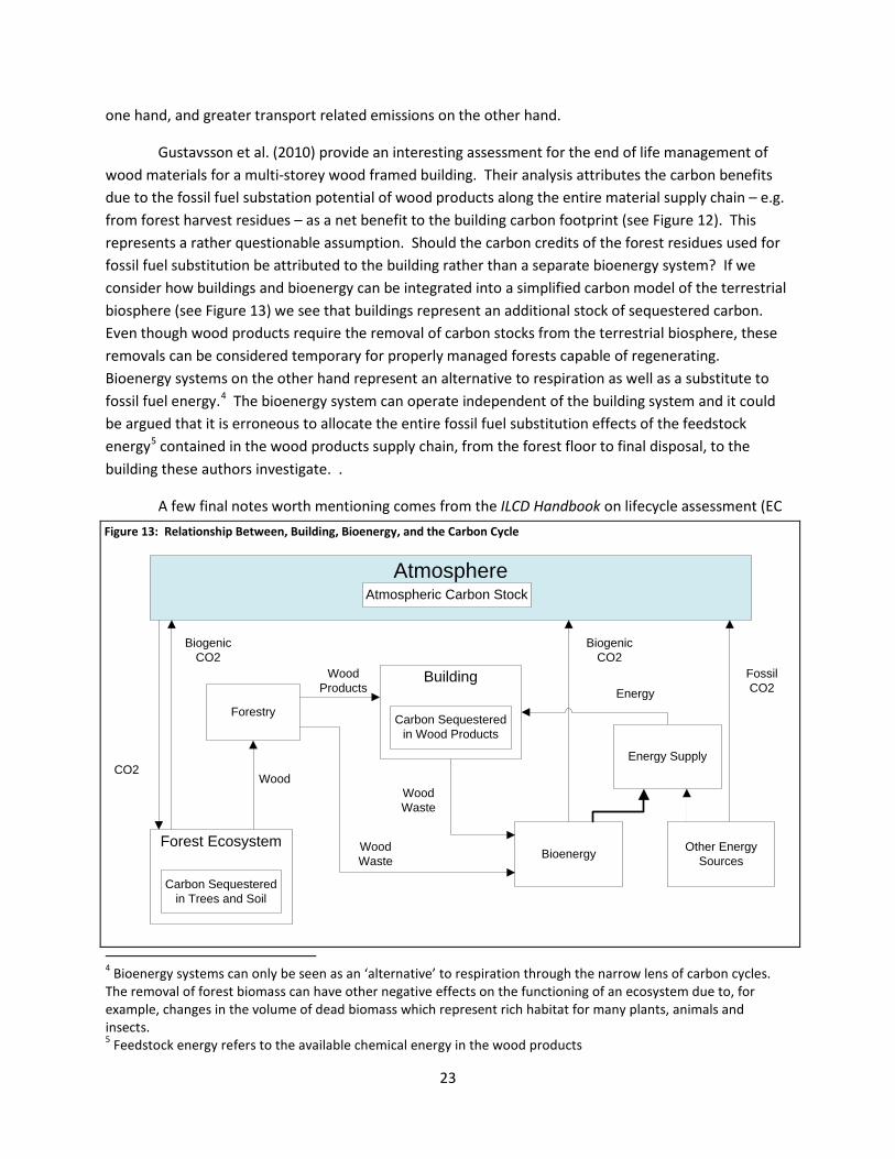
Gustavsson et al. (2010) provide an interesting assessment for the end of life management of wood materials for a multi-storey wood framed building. Their analysis attributes the carbon benefits due to the fossil fuel substation potential of wood products along the entire material supply chain – e.g. from forest harvest residues – as a net benefit to the building carbon footprint (see Figure 12). This represents a rather questionable assumption. Should the carbon credits of the forest residues used for fossil fuel substitution be attributed to the building rather than a separate bioenergy system? If we consider how buildings and bioenergy can be integrated into a simplified carbon model of the terrestrial biosphere (see Figure 13) we see that buildings represent an additional stock of sequestered carbon. Even though wood products require the removal of carbon stocks from the terrestrial biosphere, these removals can be considered temporary for properly managed forests capable of regenerating. Bioenergy systems on the other hand represent an alternative to respiration as well as a substitute to fossil fuel energy.4 The bioenergy system can operate independent of the building system and it could be argued that it is erroneous to allocate the entire fossil fuel substitution effects of the feedstock energy5 contained in the wood products supply chain, from the forest floor to final disposal, to the building these authors investigate. .

A few final notes worth mentioning comes from the ILCD Handbook on lifecycle assessment (EC

4 Bioenergy systems can only be seen as an ‘alternative’ to respiration through the narrow lens of carbon cycles. The removal of forest biomass can have other negative effects on the functioning of an ecosystem due to, for example, changes in the volume of dead biomass which represent rich habitat for many plants, animals and insects. 5 Feedstock energy refers to the available chemical energy in the wood products

Figure 13: Relationship Between, Building, Bioenergy, and the Carbon Cycle

Forest Ecosystem

Carbon Sequestered in Trees and Soil

Building

Carbon Sequestered in Wood Products

Forestry

AtmosphereAtmospheric Carbon Stock

BioenergyWood Waste

Wood Waste

Energy Supply

Other Energy Sources

CO2Wood

Biogenic CO2

Fossil CO2Energy

Wood Products

Biogenic CO2

24

JRC IES 2010) which outlines common errors to avoid in modelling waste management in LCA. One common error is the exclusion of recycling or final deposition by keeping the relevant waste flows in the LCI. Another error, particular for modelling recovery activities, involves double counting as a result of carless attention to system boundaries. For the reinforcing steel used in columns and beams, for example, it is inappropriate to allocate end-of-life recycling benefits to the system for avoided primary steel production when a ‘credit’ in the form of avoided primary steel production is already imbedded in the original production of reinforcing steel.

2.3 System Boundary Optis and Wild (2010) point out that the assembly phase almost always includes the building

structure and envelop, while mechanical systems and interior finishes are generally not and that this leads to potentially significant underestimations of the embodied energy. Given practical limitations of time which narrow the system boundaries of individual building LCAs, excluding such systems will remain common until evidence of their significance suggests otherwise.

2.4 Summary The review of the literature suggests that the operation phase of buildings remains the most

significant. Connected to this is thus the importance of the electricity supply used in the analysis. As clean electricity sources remain in short supply, reducing electricity use in clean energy economies like Norway generates real opportunities for selling this clean electricity in other markets reducing their reliance on fossil fuels. While the use of long-run marginal emissions factors would b e the golden standard for consequential modelling for long-lived products like buildings, in the meantime, it was suggested that regional emissions factors can act as a proxy.

Finally, it was also suggested by some authors that waste treatment is often inadequately modelled in building LCA studies while technical installations are often ignored altogether.

25

3 Data & Methods As described in the introduction, the general procedure for undertaking a lifecycle assessment

includes: 1) identifying the scope and system boundaries, 2) developing a lifecycle inventory, 3) impact assessment, and 4) interpretation of the results. The data and methods section presented below is structured along these lines.

3.1 Case Description: Scope and System Boundary As mentioned above, the scope of the project consists of a whole building LCA of the

Kunnskapssenter at St. Olav’s Hospital, a building currently under construction which is to be jointly owned by the hospital and the NTNU. The building consists of 17354 m2 of heated floor area including 6661 m2 of Hospital and 10693 m2 of University building space6. While Norwegian regulations require hospital buildings to consume no more than 300 kWh/m2/year and university buildings to consume no more than 160 kWh/m2/year, the passive house design standards for the hospital project estimate 168 kWh/m2/year for the hospital floor area, and 97.1 kWh/m2 for the university floor area according to the energy model data from 14-09-2009.

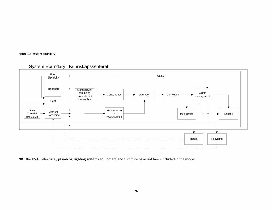
The system boundaries of the Kunnskapssenter building LCA are depicted in Figure 14 and include raw material extraction, manufacture of building components and assemblies, building construction, maintenance and replacement of components throughout the building lifecycle, building operation, demolition and all associated transport processes. As noted in the literature review, however, practical constraints of time and data often lead to either simple representations of the overall system, or to narrowing the scope to a particular subsystem of the overall building (e.g. Kim, 2011). In this study, heating ventilation and air conditioning systems, plumping and electrical (including lighting and technical equipment), and furniture were excluded due to time limitations.

3.2 Data Sources For developing the life cycle inventory (LCI) it is useful to distinguish between the foreground

system, what is explicitly modeled in the study, and the background system, which relies on data sources such as scientific literature, industry reports and life cycle inventory databases. Ecoinvent v2.2 (ecoinvent Centre, 2010) and other databases contained within the commercial LCA software SimaPro 7.3.2 (PRé Consultants, 2011) are used to model the background system including: material extraction, the manufacture of products, electricity mixes and upstream transportation processes. SimaPro is useful because it also incorporates many infrastructure processes connected to the material or process of interest. For gravel products, for example, a small proportion of the machinery used to operate gravel pits are also integrated into each unit of gravel produced (Kellenberger et al., 2007).

6 This area includes technical

26

Figure 14: System Boundary

Recycling

Waste managementDemolitionOperationConstruction

Maintenance and

Replacement

Material Processing

Transport

Heat

Fuel/Electricity

Raw Material

ExtractionIncineration

Reuse

Manufacture of building

products and assemblies

System Boundary: Kunnskapssenteret

Landfill

waste

NB: the HVAC, electrical, plumbing, lighting systems equipment and furniture have not been included in the model.

27

Primary data sources for the foreground system in this study include: 1) material volume estimates from the quantity take-off of the BIM model7, 2) architectural drawings 3) the energy model for the operation phase of the building, 4) scientific literature about Trondheim’s district heating system, and 5) maintenance and replacement schedules from SINTEF Byggforsk (2010b), 6) material densities from various sources, and 7) internet sources for estimating transport distances for building materials.

3.3 Lifecycle Inventory One innovative aspect of this thesis is the use of Building Information Modeling (BIM) for

deriving the material estimates required for building construction. Representing the last building of a 12 year construction project at St. Olav’s hospital in Trondheim, Norway, the Kunnskapssenter is the only building from this project to be modeled using BIM (Helsebygg Midt-Norge, 2012). As a rule, all new government buildings in Norway are required to use BIM starting in 2010 in an effort to improve lifecycle management of buildings and reduce costs (Statsbygg, 2007). Given enough time, one might expect software engineers to capitalize on this information revolution to assist in providing rapid, whole building LCAs.

In this study, the lifecycle inventory for the material requirements of the various building sub systems (e.g. façade, structure, interior walls, etc.) within the Kunnskapssenter are established primarily using volume estimates of the components (e.g. walls, columns, doors, etc.) extracted from the Building Information Model (BIM) in combination with estimates for the material composition of these components (e.g. of concrete or reinforced concrete) (Stadel et al., 2011). Wherever possible, technical drawings of the Kunnskapssenter are used to guide assumptions regarding the material composition of composite objects.

3.3.1 Material Densities The unit from the quantity-takeoff generated by the BIM provides volume estimates based on the 3-dimensional structure of the material. Units in Simapro, on the other hand, are often in mass. Material densities used for converting between volume and mass are provided in Appendix A: Material Densities. Where mass-ranges are given, the midpoint was used for the analysis.

3.3.2 Transport Distances Transport from product manufacturers to the building site were estimated using an internet search of product manufacturers and site visits to identify specific suppliers through packaging material. Transport distances are expected to be conservative since regional suppliers were assumed when specific information for a given product supplier was not available. Transport distances within the background data (e.g. ecoinvent v2.2) were changed for glazing production to account for the fact that the flat glass used to produce windows has not existed in Norway since the closure of Drammen Glasverk in 1977 (Wikipedia, 2012). The map in Figure 15 shows the location of European flat glass producers. For all other products, transport distances in the background data remain unchanged.

7 The BIM model was in the final stages of development during this semester. The quantity takeoff used for this analysis was received Feb. 29th 2012 and corroborated later with a take-off from March 29th and visually with a BIM model from March 29th 2012.

28

Appendix B: Transport Distances, contains transport distances, data sources, suppliers and transport assumptions for construction materials.

Assumptions for products with unknown origin were assumed to originate from local (i.e. Trondheim area), Norwegian, European or International markets. Greater detail on transport distances is provided throughout the LCI below.

3.3.3 Maintenance and Replacement Maintenance and replacement work was based on the schedules from SINTEF Byggforsk (2010b). The medium lifetime of short, medium and long maintenance and replacement estimates was used. Replacement and maintenance was inventoried using the following equation:

0.5bp

p

lrl

= −

Where, , bp lr is the number of replacements of product p , with product lifetime pl over the assumed

building lifetime bl . While not an optimal solution, the – 0.5 exists to 1) avoid the illogical result of

undertaking maintenance and replacement activity the year the building is demolished (i.e. when pl / bl

is a whole number), and 2) as a rough approximation that at time pl , 50% of the product is expected to

have been replaced assuming a normal distribution for the replacement lifetime. Essentially the – 0.5 is

Figure 15: European Flat Glass Producers in 2010

Source: Glass for Europe (N.d.) citing Nippon Sheet Glass Group (2010)

29

a decision support criteria deferring investment in maintenance as the building approaches the end of its lifetime. To demonstrate results, with a building lifetime of 30, 60, and 75 years, the ratio of doors with a lifetime of 30 years that would be replaced throughout the building lifetime would be 0.5, 1.5, and 2.0 respectively over a time span of 1, 2 and 2.5 average product lifetimes.

3.3.4 Electricity Mix The energy supply for the Kunnskapsenteret includes electricity as well as heat from the district

heating system. As the building has not yet been completed, the estimates for energy use are based on energy modeling data provided by Cowi AS (2009). The energy model was developed using SIMIEN version 5.006 (Program Byggerne ANS, n.d.). The energy requirements for various final use categories as well as delivered energy from electricity and district heating are presented in Table 1. The three column on the right represent the data that was provided. Total energy use by each category in Table 1 (the right three columns) is found using the hospital and university heated floor area which are 6601 m2 10 693 m2 respectively. Due to the small discrepancy between the total energy use estimated in this way and the total supply figures shown in the table above, they total use by process was scaled down using the energy supply values.8

The NORDEL electricity mix (see Table 2), representing the Nordic electricity market, is used for operational electricity use. The electricity mix used for material production was also changed to NORDEL for all direct material inputs (e.g. the production of windows, planed wood, etc.) in addition to the indirect inputs for steel, aluminum and forestry products. As discussed in the literature review, this

8 This discrepancy is likely a result of energy use or supply that were not updated.

Table 1: Energy Consumption: End Use and Supply

Energy uses Hospital

(kWh/m²/y) University (kWh/m²/y)

Total Hospital (scaled)

Total University (scaled)

Assumed Supply

1a Space heating 11,4 7,5 74702 78054 District Heat 1b Ventilation Heat (thermal batteries) 2,0 3,1 13106 32262 District Heat 2 Hot water (tap water) 29,8 5 195274 52036 District Heat 3a Fans 30,6 17,7 200516 184208 Electricity 3b Pumps 3,2 2,9 20969 30181 Electricity 4 Lighting 30,4 18,8 199205 195656 Electricity 5 Technical Equipment 46,7 34,5 306016 359050 Electricity 6a space cooling 0,0 0 0 0 6b Ventilation Cooling 14,0 7,7 91739 80136 Electricity 7 Total net energy 168,1 97,2 1101527 1011584 Regulated requiement 300 160 Total Annual Energy Supply (kWh) Electricity 819770 834330 District Heating 281757 177254 Total 1101527 1011584

Total heated floor area = 17354 m2 Source: (Cowi AS, 2009)

30

decision is grounded, on the one hand, in the realities of an interconnected electricity market, and on the other hand, that this interconnection has the potential to increase substantially in the future through the implementation of future energy scenarios in countries like Germany (German Advisory Council on the Environment, 2011).

3.3.5 District Heating System The fuel mix supplied to the district heating system for 2009 was used in this assessment (see

Table 3) (Brattebø & Reenaas, 2012). Given the lack of inventory for landfill gas, liquefied propane gas was assumed instead. Due to the small fraction of landfill gas (i.e. << than one percent) this decision is assumed to be negligible on the results.

As mentioned above in the literature review, ecoinvent allocates 100% of the emissions from waste incineration to the waste disposal function and 0% to the energy production function. The reference scenario in this assessment takes the opposite approach allocating 100% of the emissions to heat production. Since waste for the use phase was not inventoried, shifting the allocating from waste disposal to heat production shifts the system boundaries to provide a more complete picture of the building life cycle9.

Allocating the emissions from waste to heat production altering the ecoinvent v2.2 process “heat from waste, at municipal waste incineration plant” to include the output “disposal, municipal solid waste, 22.9% water, to municipal incineration”. Further, it was necessary to change the quantity of waste heat from the disposal process. The ecoinvent process for waste disposal via incineration is based on electricity and heat production where the waste heat from electricity is inventoried in the electricity 9 A shortfall of this approach for a hospital building is that the hazardous waste incinerated at hospitals is not properly inventoried.

Table 2: NORDEL Electricity Mix

Electricity source DK FI NO SE Total share hard coal 45,7 % 19,1 % 0,0 % 0,7 % 9,0 % oil 4,0 % 0,7 % 0,0 % 1,3 % 1,1 % natural gas 24,5 % 14,8 % 0,3 % 0,5 % 6,0 % hydropower 0,1 % 17,9 % 98,5 % 40,1 % 48,1 % wind power 17,2 % 0,1 % 0,3 % 0,6 % 2,1 % cogen ORC 1400kWth, wood, allocation exergy 4,5 % 11,8 % 0,3 % 4,4 % 4,8 % cogen with biogas engine, allocation exergy 0,6 % 0,0 % - 0,1 % 0,1 % peat - 7,6 % - 0,5 % 1,8 % industrial gas - 0,6 % 0,0 % 0,5 % 0,4 % nuclear - 26,7 % - 50,5 % 25,6 % hydropower - - 0,5 % 0,1 % 0,2 % NORDEL Production share 10,2 % 21,6 % 29,0 % 39,3 % DK = Denmark; FI = Finland; NO = Norway; SE = Sweden

Source: ecoinvent v2.2 (ecoinvent Centre, 2010)

31

producing process and all other heat is inventoried in the disposal function (Doka, 2009). For 1 kg of waste disposal, 83% of the energy based on the higher heating value (13.27 MJ/kg) is inventoried as waste heat to air and 17% is inventoried as waste heat to water based on air and water throughputs (Doka, 2009). The share of biogenic carbon in the waste is left at 60.4%. The lower heating value for municipal solid waste incineration in the documentation tab in SimaPro is listed as 11.74 MJ/kg. The thermal conversion efficiency is set to 85% (Brattebø & Reenaas, 2012) which is substantially higher than the conversion efficiencies of 13% for electricity and 25.7% for thermal energy suggested in the SimaPro documentation tab for the disposal of municipal solid waste. Brattebø & Reenaas (2012) also state a 10% heat loss in the distribution pipes.

The processes used to inventory the heating fuels can be found in Appendix E: Process Summary, Table 2.

3.3.6 Structural System The structural system is here defined as the foundation, floor slabs, walls, beams, columns and associated components. The volume estimates for the materials used in these components are presented in Table 4. The load bearing walls presented in this section, as opposed to the section on interior partitions, refer mainly to walls used in the underground floors, elevator shafts, and staircases. The main use of insulation in the load bearing walls is contained in the middle of reinforced concrete ‘sandwich walls’ which separate the elevator shafts and staircases from large exhaust stacks on the exterior of the building. This insulation is assumed to be half expanded polystyrene (EPS), and half extruded polystyrene (XPS).

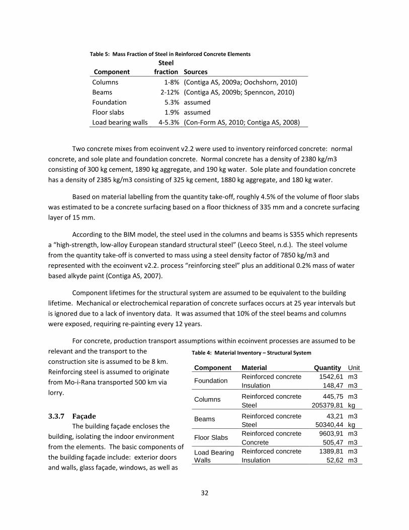
As determined from literature sources, the mass fraction of steel contained within reinforced concrete columns, beams, foundations, floor slabs and walls is shown in Table 5. In this study the mass fraction of steel used for these elements were: .4.5% (columns), 7% (beams), 5.3% (foundation), 1.9% (floor slabs), and 4% (walls). The ecoinvent v2.2 process “reinforcing steel” has a material composition of 63% “steel converter, unalloyed” and 37% “steel electric, un- and low-alloyed”. Converter steel contains approximately 19% iron scrap while electric steel contains 100% iron scrap for a total of approximately 49% recycled scrap in the process. However, documentation from The Norwegian Environmental Product Foundation and personal communication with Paulik (2012) suggests that the scrap content in reinforced steel products is 76-80%. Reinforcing steel was inventoried throughout this analysis as 27% converter steel, and 23% electric steel. Further, the electricity mix for hot rolling, converter steel and electric steel was adjusted from a European mix to a Nordic mix.

Table 3: Trondheim District Heat Energy Supply Mix

Heat Source 2009 Mix Waste incineration 69,70 % Biofuels 4,27 % Heat pumps 0,58 % Landfill gas 0,05 % Natural gas 2,99 % Propane and butane gas 12,07 % Fuel oil 1,09 % Electricity 9,24 %

Source: (Brattebø & Reenaas, 2012)

32

Two concrete mixes from ecoinvent v2.2 were used to inventory reinforced concrete: normal concrete, and sole plate and foundation concrete. Normal concrete has a density of 2380 kg/m3 consisting of 300 kg cement, 1890 kg aggregate, and 190 kg water. Sole plate and foundation concrete has a density of 2385 kg/m3 consisting of 325 kg cement, 1880 kg aggregate, and 180 kg water.

Based on material labelling from the quantity take-off, roughly 4.5% of the volume of floor slabs was estimated to be a concrete surfacing based on a floor thickness of 335 mm and a concrete surfacing layer of 15 mm.

According to the BIM model, the steel used in the columns and beams is S355 which represents a “high-strength, low-alloy European standard structural steel” (Leeco Steel, n.d.). The steel volume from the quantity take-off is converted to mass using a steel density factor of 7850 kg/m3 and represented with the ecoinvent v2.2. process “reinforcing steel” plus an additional 0.2% mass of water based alkyde paint (Contiga AS, 2007).

Component lifetimes for the structural system are assumed to be equivalent to the building lifetime. Mechanical or electrochemical reparation of concrete surfaces occurs at 25 year intervals but is ignored due to a lack of inventory data. It was assumed that 10% of the steel beams and columns were exposed, requiring re-painting every 12 years.

For concrete, production transport assumptions within ecoinvent processes are assumed to be relevant and the transport to the construction site is assumed to be 8 km. Reinforcing steel is assumed to originate from Mo-i-Rana transported 500 km via lorry.

3.3.7 Façade The building façade encloses the building, isolating the indoor environment from the elements. The basic components of the building façade include: exterior doors and walls, glass façade, windows, as well as

Table 4: Material Inventory – Structural System

Component Material Quantity Unit

Foundation Reinforced concrete 1542,61 m3 Insulation 148,47 m3

Columns Reinforced concrete 445,75 m3 Steel 205379,81 kg

Beams Reinforced concrete 43,21 m3 Steel 50340,44 kg

Floor Slabs Reinforced concrete 9603,91 m3 Concrete 505,47 m3

Load Bearing Walls

Reinforced concrete 1389,81 m3 Insulation 52,62 m3

Table 5: Mass Fraction of Steel in Reinforced Concrete Elements

Component Steel

fraction Sources Columns 1-8% (Contiga AS, 2009a; Oochshorn, 2010) Beams 2-12% (Contiga AS, 2009b; Spenncon, 2010) Foundation 5.3% assumed Floor slabs 1.9% assumed Load bearing walls 4-5.3% (Con-Form AS, 2010; Contiga AS, 2008)

33

aluminum and glass cladding which cover the exterior walls. The steel exhaust stacks for the building were also inventoried with the façade system.

3.3.7.1 Exterior walls The two main exterior

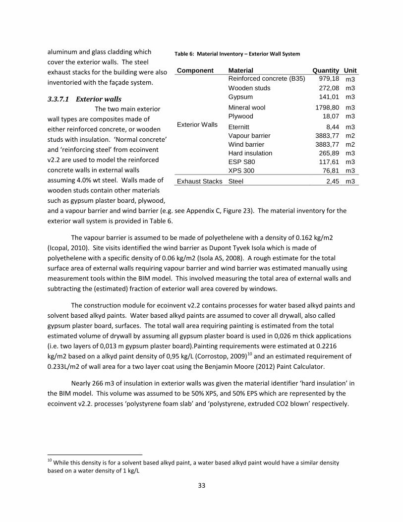
wall types are composites made of either reinforced concrete, or wooden studs with insulation. ‘Normal concrete’ and ‘reinforcing steel’ from ecoinvent v2.2 are used to model the reinforced concrete walls in external walls assuming 4.0% wt steel. Walls made of wooden studs contain other materials such as gypsum plaster board, plywood, and a vapour barrier and wind barrier (e.g. see Appendix C, Figure 23). The material inventory for the exterior wall system is provided in Table 6.

The vapour barrier is assumed to be made of polyethelene with a density of 0.162 kg/m2 (Icopal, 2010). Site visits identified the wind barrier as Dupont Tyvek Isola which is made of polyethelene with a specific density of 0.06 kg/m2 (Isola AS, 2008). A rough estimate for the total surface area of external walls requiring vapour barrier and wind barrier was estimated manually using measurement tools within the BIM model. This involved measuring the total area of external walls and subtracting the (estimated) fraction of exterior wall area covered by windows.

The construction module for ecoinvent v2.2 contains processes for water based alkyd paints and solvent based alkyd paints. Water based alkyd paints are assumed to cover all drywall, also called gypsum plaster board, surfaces. The total wall area requiring painting is estimated from the total estimated volume of drywall by assuming all gypsum plaster board is used in 0,026 m thick applications (i.e. two layers of 0,013 m gypsum plaster board).Painting requirements were estimated at 0.2216 kg/m2 based on a alkyd paint density of 0,95 kg/L (Corrostop, 2009)10 and an estimated requirement of 0.233L/m2 of wall area for a two layer coat using the Benjamin Moore (2012) Paint Calculator.

Nearly 266 m3 of insulation in exterior walls was given the material identifier ‘hard insulation’ in the BIM model. This volume was assumed to be 50% XPS, and 50% EPS which are represented by the ecoinvent v2.2. processes ‘polystyrene foam slab’ and ‘polystyrene, extruded CO2 blown’ respectively.

10 While this density is for a solvent based alkyd paint, a water based alkyd paint would have a similar density based on a water density of 1 kg/L

Table 6: Material Inventory – Exterior Wall System

Component Material Quantity Unit

Exterior Walls

Reinforced concrete (B35) 979,18 m3 Wooden studs 272,08 m3 Gypsum 141,01 m3 Mineral wool 1798,80 m3 Plywood 18,07 m3 Eternitt 8,44 m3 Vapour barrier 3883,77 m2 Wind barrier 3883,77 m2 Hard insulation 265,89 m3 ESP S80 117,61 m3 XPS 300 76,81 m3

Exhaust Stacks Steel 2,45 m3

34

Transport distances include for locally produced products include: Rockwool (6 km), XPS/EPS (12 km – Brødr. Sunde AS11). Transport distances for other Norwegian products include: drywall (575 km – Drammen and Fredrikstad), Aluminum (750 km), plywood (440 km), lumber (152 km). What about vapour barrier, wind barrier, and eternett?

3.3.7.2 Cladding As illustrated in the bottom part of the technical drawing in Appendix C, Figure 23, exterior walls

are often covered with cladding. The major cladding materials used in the Kunnskapcsenter include glass and aluminum. The aluminum cladding is made of 3mm natural anodized aluminum, while the glass cladding is fastened using vertical aluminum supports. The glass used for the glass cladding is assumed to be 1 cm thick. Additional aluminum siding is used for the perimeter of the building to cover the transition between floors, and to cover the parapets along the crown of the building. Finally, treated wood is used to shade the bridges which connect to neighbouring buildings. Table 7 quantifies the material requirement for cladding.

In the BIM model the fasteners for the glass cladding are modeled as solid aluminum objects with a cross sectional area of 40 cm2. It is assumed that these fasteners are hollow objects with a 3mm thick outer edge. The density of glass is taken to be 2600 kg/m3 (The Engineering Toolbox, n.d.). Following (Dahlstrøm, 2010) the glass panels are assumed to originate from Germany, which, as pointed out above in the transport section represents the closest flat glass producers12. The total transport distance is assumed to be 1030 km – a 150 km transoceanic shipment between Norway and Denmark and 880 km by lorry.

The density of aluminum is 2712 kg/m3 (The Engineering Toolbox, n.d.). According to Liu (Liu, 2012) aluminum products in Europe are generally cascaded from wrought products made of primary aluminum into lower quality alloys with aluminum building products mainly using primary aluminum. Aluminum cladding is assumed to be made of primary aluminum originating from within Norway. The average transport distance for aluminum products is assumed to be 750 km taking into account production facilities in Husnes (800 km), Høyanger (650 km), Sunndal (750 km), Årdal (850 km). Assuming aluminum for the Trondheim building market is served equally by these production facilities the average transport distance is roughly 750 km by Lorry.

11 According to wikipedia, Brødr. Sunde AS is the largest producer of EPS products in Scandinavia with several production facilities including one located just outside of Heimdal in the Suburbs of Trondheim. 12 According to wikipedia, the production of flat glass in Norway came to and end in 1977 with the closure of Drammen glasverk.

Table 7: Material Inventory – Cladding

Component Material Quantity Unit

Cladding

Aluminum cladding 11326,1 kg Glass cladding 33752,3 kg Fasteners (alu.) 3187,6 kg Treated wood siding 41,3 m3

Parapet Aluminum cladding 9772,6 kg Floor transitions Aluminum siding 22332,4 kg

35

3.3.7.3 Fenestration The term fenestration is used here to refer to the portion of the façade composed of windows, doors and the glass curtain wall.

Glazing Units The low-energy design standards for the building require window U-values of 0.8 W/m2K (Cowi

AS, 2009). The econinvent database has a process for triple glazed units with a U-value of 0.5 W/m2k (Kellenberger et al., 2007). The cladding and window frame processes described below bring the U-value up closer to 0.8 W/m2K.

Transport distances for glazing units from the producer to the building site are estimated at roughly 100 km based on the window supplier’s production factory in Lian East of Trondheim. According to their website, their glass suppliers include Pilkington Glass – with the nearest production facilities in Halmstad, Sweden, and Dortmund, Germany – and Press Glass which has factories located in Poland. Based on these assumptions, transporting flat glass from the flat glass producers to the window producer in Lian are estimated using google maps to include 1600 km Lorry transport and 100 km transoceanic shipment.

Windows There are 348 windows in the external façade represented by 7 different sizes13. The glazed

area, window frame area, glass covering, and number of windows for each window size are provided in Table 9. The glass covering, estimated to be 4 mm thick, is a small covering at the bottom of many windows which acts as a cladding surface covering an exterior wall. The windows are modeled using the previously mentioned process for glazing units, and an ecoinvent v2.2 process for aluminum window frames with a U value of 1.6 W/m2K.

According to the process for aluminum window frames, 1 m2 of visible aluminum window frame weighs 50.7 kg. Given the estimated mass of the glazing unit above, the total mass of transported window products is provided in Table 9. Transport distances for windows is based on previously stated estimates for glazing units.

Thus far the external windows shades have not been included in the model due to a lack of lifecycle data.

Glass Curtain Wall The glass curtain wall consists of a triple glazed window system with aluminum mullions which

are the framing elements separating adjacent windows. While the BIM distinguishes between the aluminum mullions and the glazing units, the ecoinvent v2.2 process for “cladding, crossbar pole, aluminum” which describes 1 m2 of a curtain wall system with triple glazed windows and aluminum/steel mullions with a specific mass of 55.77 kg/m2

13 The 7 window sizes modeled here represent a simplification of actual window sizes.

Table 8; LCI – Curtain Wall

Component Material Quantity Unit

Glass Curtain Wall Glazing units 2551 m2 Mullions 147,5 m2

36

(Kellenberger et al., 2007)14. This assumption was used because the aluminum mullions were modeled as solid objects in the BIM model and life cycle data for aluminum mullions (see e.g. Figure 16) was not readily available.

The unit process “cladding, crossbar pole, aluminum” includes an estimated 0,667 m2 glazing compared to the approximately 94.5% glazing quantified in Table 8. To adjust for this discrepancy, the input of glazing into the ‘cladding’ process was adjusted to 97.3 to account for the waste fraction in the process (~2%) as well an assumed 1% hidden glazing unit around the edges (Kellenberger et al., 2007). The quantity of other materials in the process are assumed to be constant which could be accounted for by having deeper mullions that go further into the wall. This final assumption is thought to be conservative since it is unlikely that less aluminum and steel is required to support more glazing.

Transport distances for glazing units are the same as in previous sections. Transport distances for steel and aluminum for the mullions to the curtain wall production facility, which is assumed to be located in Trondheim, are 500 km and 750 km as in previous section plus 15 km local transport to the 14 NB: 55.77 kg/m2 is a correction from the stated mass of 80.7 kg/m2 based on a mass balance calculation (Ruiz, May 2012, personal communication).

Table 9: Windows: Glazing Area and Window Frame Area in m2

Window Type Quantity

Gross Window

Area Glazing

Area Frame Area

Coloured Glass Area

Total Glazing

Area

Total Window Frame Area

Total Coloured

Glass Area

Total Mass (kg)

Glazing mass (kg)

Frame Mass (kg)

Coloured Glass Mass (kg)

1 1,0 1,1 0,9 0,2 0,0 0,9 0,2 0 37 27 10,14 0 2 9,0 1,1 0,9 0,2 0,0 8,3 2,0 0 349 248,4 100,39 0 3 35,0 1,6 1,3 0,2 0,0 45,9 8,4 0 1801 1375,5 425,88 0 4 138,0 2,7 2,0 0,4 0,3 281,5 59,3 42,78 11839 8445,6 3008,5 385 5 153,0 3,8 2,9 0,5 0,5 440,6 71,9 70,38 17498 13219 3645,8 633 6 8,0 5,8 4,4 0,7 0,7 34,9 5,9 5,6 1397 1046,4 300,14 50 7 4,0 7,8 5,7 1,5 0,5 22,9 6,1 2,16 1014 686,4 308,26 19

Total 835,0 153,8 120,92 33936 25049 7799 1088 30,0 mass of glazing unit (kg/m2) 50,7 mass of window frame (kg/m2) 9,0 mass of coloured glass (kg/m2)

Figure 16: Aluminum Mullion

Source: The Virtual Architecture Exhibition (N.d.)

37

building site.

Outer Doors The 52 outer doors are glazed doors with

aluminum frames. Due to a lack of inventory data on aluminum framed doors, they are treated analogously to aluminum framed windows with the total estimated mass of the frame and window provided in Table 10.

3.3.8 Interior partitions The interior partitions include interior walls,

windows and doors. The total material estimate for interior walls is presented in Table 11.

Walls The BIM model contains 36 different wall types. However, roughly 87% of the volume from interior walls is represented by just 5 wall types. Cross.sectional architectural drawings were available for 18 of these wall types (see Appendix C, Figure 24 and Figure 25). These cross-sectional wall specifications combined with material labelling in both the quantity take-off and BIM model provided the basis for estimating the material composition of interior walls. For several wall types, for example for wall type 241.01, the BIM model and quantity take-off indicated that several walls of a particular type were made of concrete which is assumed to be reinforced concrete with a steel fraction of 5.3% wt. Approximately 25% of interior walls were estimated to be made of reinforced concrete.

For estimating the material composition of walls with steel and wood studs, the stud spacing was assumed to be 30 cm plus supportive studs along the top and bottom of each wall which, in general, are assumed to have an average height of 3 m. The depth of the studs were determined from the architectural drawings. The steel studs were assumed to be made of galvanized steel sheets 0.959 mm thick which includes a 0,04 mm layer of zinc (Canadian Sheet Steel Building Institute, 2006). For insulated walls, insulation was assumed to fill the empty cavity of the steel studs.

The relatively small amount of veneer is assumed to be medium density fibre (MDF) board due to lack of LCI data.

Transport of steel studs is assumed to be the same as other steel products – 500 km from Mo I Rana to Trondheim.

Maintenance included repainting the drywall every 12 years including 15 km transport to site.

Table 10: Outer Door Types

Door Type Quantity

Gross Door area

Glazing Area

Door Blade Area (m2)

Total glazing Area (m2)

Total Door Blade Area (m2)

Total Mass (kg)

1 10 5,56 3,36 2,2 33,6 22 1628 2 16 2,67 1,6 1,07 25,6 17,12 913 3 12 4,47 2,56 1,91 30,72 22,92 1354 4 14 3,7 1,9 1,8 26,6 25,2 1136

Total 116,5 87,24 5031

Table 11: LCI – Interior Walls

Material Quantity Unit Reinforced Concrete 738,79 m3 Galvinized Steel 10,18 m3 Wood Studs 4,76 m3 Insulation (mineral wool) 355,05 m3

Drywall 665,08 m3 Plywood 4,11 m3 Light Weight Aggregate 12,15 m3 Plaster 1,21 m3 Veneer (MDF) 13,71 m3 Vindspere 1,82 m2 *Veneer assumed to be MDF at present

38

Interior Curtain Wall The interior

curtain wall consists of sound-proof glazing, single pane glazing, doors, and aluminum and wood mullions. The quantity estimates for interior windows, mullions and doors is provided in Table 12.

The materials used for doors integrated into the curtain wall is unknown and is assumed to be represented by the ecoinvent processes “door, inner, wood-glass). While only 33% of the surface area for the ecoinvent process for wood-glass doors is glass vs 44% of the door surface area in the BIM model, this was assumed to be sufficient for a first estimate.

The quantity take-off for Interior windows generates a volume. The thickness of interior windows was estimated, using BIM measurement tools, to be roughly 2 cm thick. Sound proof windows are assumed to be double glazed windows for the LCI. For a noise over 60 dB, for instance, Glasfabrikken (N.d.) provides a double glazed window consisting of one 6 mm and one 4 mm glass panel. In the case of non-soundproof windows, the Simapro process for double glazing is adjusted to represent a single glazed window (see Appendix E: Process Summary, Table 30) – i.e. to include manufacturing energy and cleaning water. The aluminum glazing bars are modeled as hollow aluminum objects with a 3mm profile, while the wood glazing bars are modeled as planed, sawn timber with a coat of varnish. With cross-sectional dimensions of 29 mm x 100 mm, the wood glazing bars are estimated to have a surface area of 338 m2 for the varnish coat. The varnish inventory was estimated using values for the wooden frame of the ecoinvent process ‘door, inner, wood, at plant’, and includes 0.614 kg of acrylic filler, 9.24 kg of acrylic dispersion and 9.24 kg of acrylic varnish per m3 of wood mullion (Kellenberger et al., 2007).

Maintenance included painting the wood mullions and door blades every 8 years.

Interior Doors There are 633 inner doors in addition to the doors contained in the interior curtain wall. The

labelling system for the doors used in the BIM model suggests that all doors not integrated into the interior curtain wall system have a steel door frame with a mix of door blades made of either steel or

Table 12: LCI – Interior Curtain Wall & Doors

Component Material Quantity Unit

Curtain wall

Sound proof glazing (double glazing) 2446 m2 Single pane glazing 866 m2 Door window area 231,8 m2 Door blade area 295,3 m2 Aluminum mullion 5x100 mm 0,075 m3 Aluminum mullion 30x100 mm 0,752 m3 Mullion powder coating area 31,5 m2 Wood Mullion 29x100 mm 3,8 m3 Wood mullion varnish area 338,1 m2

Steel-framed doors

Laminate door, blade 814,9 m2 Laminate door, glass 72,9 m2 Steel door, blade 284,5 m2 Steel door, glass 54,7 m2 Unknown door blade area (assume laminate) 80,5 m2 Unknown door, glass area 13,7 m2 Glass door 15,5 m2

Total door area requiring steel door frames 1336,8 m2

39

‘laminate’ plus glass. The wood and aluminum mullions described above in the curtain wall system provide the door frames for doors within the curtain wall system

The laminate doors are assumed to be laminated wooden doors. The ecoinvent process “Door, inner, wood, at plant/RER U” is used to represent 1 m2 of laminated wooden doors (See Kellenberger et al., 2007). However, since this process includes a wooden door frame, an adjustment is necessary which subtracts the processes used in the manufacture of the wooden door frame. After this adjustment, the wooden door is estimated to weigh 17.43 kg/m2 based on a subtraction of 0.0203 m3 for the wooden frame, assuming a softwood density of 500 kg/m3 (The Engineering Toolbox, n.d.), and an original unit mass of 27.6 kg/m2. Maintenance included re-painting the door blade every 8 years.

The steel frame for 1 m2 of door is extracted from the ecoinvent v2.2 process “door, outer, wood-aluminum, at plant/RER U”. The zinc layer applied to galvanize the outdoor steel frame is removed for interior application. The mass of the steel frame including packaging is 10.6 kg. Ecoinvent assumes a lifetime of 60 yrs for the steel door frame. Maintenance for steel door frames two layers of paint covering a surface area of 0.43 m2 per m2 of door area.

Inner steel doors were modeled by combining data from Hörmann KG Brandis (2012), Steelcraft Co. (2000) and the ecoinvent v2.2. processes “Door, inner, wood, at plant/RER U”, and “Door, outer, wood-aluminum, at plant/RER U”. The data contained in the environmental product declaration for steel doors from Hörmann KG Brandis (2012) is too vague to be directly useful. A process representing the manufacture of steel doors was therefore developed using the four data sources mentioned above. The ecoinvent v2.2 processes for inner, wood doors and outer, wood-aluminum doors were cross-checked to estimate fittings and process energy per m2 of door. The product description for steel doors taken from Steelcraft Co. (2000) was used to estimate the mass of steel required for a 1.2x2.0 door blade which was then scaled down to 1 m2. Data from this product description included: the door blade thickness (0.045 m), the steel panel thickness for each side of the door (1.7 mm), the steel processing (cold-rolled) technique, and the material composition of the honeycomb core (phenolic resin). The mass of the honeycomb core is estimated using data from the EPD by Hörmann KG Brandis (2012). This EPD provides data on the mass fraction of the materials used in the door (see Table 13). Edge construction for the steel doors is assumed to be mechanical interlocking edges Steelcraft Co. (2000). The ecoinvent process “powder coating, steel” is used to model the surface coating of the doors. For a complete inventor of the process, see Appendix E: Process Summary, Table 33. Maintenance of steel doors involved two layers of paint over an area of m2 per m2 of door area.

3.3.9 Roof The roofing systems for the Kunnskapssenter differ between the main building, and the

auditorium. The material inventory for both roofing systems is provided in Table 14.

Table 13: Material Composition of Interior Steel Doors

Material Mass

Fraction Steel 90,20 % Honeycomb insert (phenolic resin) 4,00 % Plastic 2,20 % Wood 1,90 % Sealing 1,10 % Paint 0,60 %

Source: (Hörmann KG Brandis, 2012)

40

The main building roofing system consists of concrete covered with mineral wool, a vapour barrier, and a sedum15 green roof supported by a wooden supportive structure (see Appendix C, Figure 26) in addition to technical rooms. Due to a lack of information in the architectural drawings, the LCI for the main roof excluded the materials for the green roof including the wood build-up. Only mineral wool was inventoried for the technical rooms due to a lack of architectural drawings for theses structures.

Rooftop hand railings were measured manually from within the BIM model and were assumed to be made of galvanized reinforcing steel using the processes “reinforcing steel” and “zinc coating, coils”. Each vertical element of the railing was spaced 11 cm apart and measured 40 mm x 4.5 mm. Supporting rails along the top and bottom had the same 40mm x 4.5 mm dimension. The total length of railings was approximately 275 m.

The parapet, which refers to the crowning element surrounding the top of the roof, was inventoried here, but included in the model as part of the façade. The volume for the parapet in the material take-off was estimated to contain approximately 63% insulation, 23% wooden studs, and 14% plywood based on 45 cm stud spacing. An additional volume of 3% was included for the anodized aluminum siding based on a sheet thickness of 3 mm. The area covered by the vapour barrier was estimated manually using measurement tools within the BIM model. Since the concrete used in the roof was indistinguishable from concrete used for floor slabs in the BIM quantity take-off, the concrete for the main roof was inventoried as part of the floor slabs. Inventoried maintenance for the main roof consisted of replacing the vapour barrier at 40 year intervals.

Details for the auditorium roof are presented in Appendix C, Figure 27. The BIM modelling for the auditorium roof was undertaken by external consultants and it was not possible to extract any information from the quantity take-off. The dimensions of the auditorium roof were extracted from technical drawings and measurement tools within the BIM model. The total surface area of the roof, excluding the atrium glass covering and skylights, was estimated to be roughly 620 m2. The zinc roof cladding was assumed to be 0.7 mm thick (Euroclad, n.d.). Given that major global zinc producers are China, Australia, Canada and the US, transport distances for zinc are assumed to be 2000 km transoceanic shipment, and 500 km by Lorry. The surface area of the second layer of insulation was scaled down to 90% of the estimated surface area (i.e. 620 m2 x 0.90) to account for the space occupied by the glulam beams. The total insulation volume was assumed to be half EPS, and half XPS. The ‘secondary supportive roof cladding’ shown in the technical drawing was assumed to be plywood and

15 According to Wikipedia, sedum is a genus of flowering plant

Table 14: LCI – Roofing Systems

Component Material Quantity Unit

Auditorium Roof

Glulam 67,77252 m3 Insulation 236,504 m3 Zinc roof cladding 0,431732 m3 Glass covering, atrium 112 m2 Plywood 27,7542 m3 Windows, skylight 63,24 m2 Vapour barrier 616,76 m2

Main Roof

Vapour barrier 5904 m2 Minerawool 1966,81 m3 Railing (steel) 0,630 m3 Railing surface area for galvzanizing 24,47 m2

41

the total plywood volume was estimated by assuming three layers 15 mm thick. The surface area of the skylight windows and glass covering for the atrium were manually estimated from the BIM model. The skylight windows were represented as aluminum framed, triple glazed windows with a 15:85 split between the window frame surface area and the glazing unit surface area. The atrium glass covering was assumed to consist of triple-glazed windows with aluminum glazing bars using the ecoinvent v2.2 process “cladding, crossbar-pole, aluminum”.

Maintenance and replacement for the auditorium roof included replacing glazing and window frames at 40 year intervals.

3.3.10 Balconies The inventory for the balconies from the quantity take-off is presented in Table 15. The material

marker for the insulation used under the balconies in the BIM model was limited to the label ‘hard’ and this volume was split evenly between EPS and XPS for the LCI. The balcony railings were identical to those on the main roof and were roughly 45 m in length. It was assumed that composition of the reinforced concrete used for balconies had a stell fraction of 1.9% wt.

3.3.11 Ceiling Coverings and Ceiling Walls Ceiling coverings and ‘ceiling walls’ for technical installations (e.g. HVAC ducts, plumping, etc.)

are inventoried in this section (see Table 16). The material inventory for ceiling coverings was complicated by incomplete material labeling within the BIM model. The material inventory consisted of approximately 17 ceiling covering types, and 5 ceiling wall types. The volume of gypsum based ceiling tiles, plywood, eternit, mineral wool and metal ceiling were manually estimated with information in the BIM material labeling and dimensions within the BIM model. Ceiling tiles were between 50-70 mm thick in the BIM model while the material label typically indicated material thicknesses in the range of 20-25 mm along with the remaining thickness unlabelled which is assumed to be empty space. The volume of metal ceiling objects was scaled down assuming 3 mm thickness. Two large steel plates, which were part of the ceiling in the main entrance, were also extracted from the quantity take-off from the BIM.

The gypsum based ceiling panels were inventoried as “gypsum plaster board”, eternity as “fibre cement facing tile”, the steel plate “reinforcing steel”, and the metal ceiling as “steel, converter, unalloyed" plus “hot rolling, steel” – all ecoinvent v2.2 processes.

Table 15: LCI – Balconies

Material Quantity Unit Reinforced concrete 3,70 m3 EPS 8,67 m3 XPS 8,67 m3 Railing 0,10 m3 Railing surface area for galvanizing 3,97 m2

Table 16: LCI – Ceiling Coverings and Walls Component Material Quantity Unit

Ceiling Panels

Drywall 225,39 m3 Plywood 3,54 m3 Mineral wool 148,76 m3 Eternitt 23,99 m3 Steel plate 2,27 m3 Metal 0,79 m3

Ceiling Walls Galvinized studs 2,11 m3 Drywall 78,88 m3 Mineral wool 14,18 m3

42

Maintenance and replacement activities included painting the gypsum panels at 12 year intervals.

3.3.12 Floor Coverings The materials inventoried for floor coverings are

listed in Table 17. Because unique identifiers were not provided for different flooring materials, the quantity take-off from the BIM model was not useful for developing an inventory for floor coverings. Instead, floor plans indicating flooring type were used to roughly estimate the total floor area of different flooring types. Since a floor plan indicating flooring materials for the 5th floor was not found, the materials from the 4th floor, which has the same floor area as the 5th floor, were doubled.

As determined from architectural drawings, the thickness of the various flooring types included: 3 mm (linoleum), 3mm (vinyl), 18 mm (terrazzo), and 22 mm (parquet). According to TileClock (2009), interior tiles are between 5.5-8.25 mm thick. Mipolam is a vinyl based flooring product with Gerflor (N.d.) listing a product for health care with a thickness of 2 mm and a density of 3.04 kg/m2.

Linoleum was inventoried using the IDEMAT 2001 process for linoleum. Vinyl and Mipolam were represented by the ecoinvent v2.2 processes “polyvinylchloride, suspension polymerised” while the process “ceramic tile” was used for ceramic tiles. The process “glued laminated timber” was used as a proxy for parquet flooring. Using the estimated parquet floor area of 58 m2, an estimated 15.7 kg of varnish is required to surface the parquet flooring based on a varnish density of 0.9 kg/L (Pereira & Bueno, 2008), and an estimated varnish requirement for wood flooring of 0.3L/m2 (Ecos Organic Paints, n.d.). Terrazzo and epoxy floorings have been excluded due to a lack of inventory data.

Vinyl and lineolum products is assumed to originate in Northern Germany travelling 1000 km by lorry and 150 km by transoceanic shipment.

The maintenance for parquet flooring requires re-varnishing every 5 years. Re-coating concrete floors with epoxy occurs every 10 years. Vinyl, linoleum and ceramic tiles require replacement every 20 years.

3.3.13 Interior wall Coverings Wall coverings from the quantity take-off include bathroom wall tiles, panels located behind

bathroom sinks which are assumed to be mirrors, and veneer. As above, tiles are inventoried as using the ecoinvent v2.2 process “ceramic tiles”. Due to a lack of inventory data, mirrors are inventoried using the ecoinvent process “flat glass”, and veneer is inventoried using the process “medium density fibre board” which is assumed to

Table 17: LCI – Floor Coverings

Material Quantity Unit Epoxy painting 833 m2 4 mm Epoxy slurry mixture 4,00 m3 Linoleum 21,24 m3 Vinyl 7,88 m3 Ceramic tile 1,84 m3 Terrazzo 49,67 m3 ESD Mipolam 0,67 m3 Parquett 1,27 m3

Table 18: LCI – Wall coverings

Material Quantity Unit Bathroom tile 14,21 m3 Bathroom mirrors 0,24 m3 Veneer 0,57 m3

43

be the base for the veneer.

Maintenance includes replacing ceramic tiles every 20 years (SINTEF Byggforsk, 2010b).

3.3.14 Stairs The material volume for stairs was estimated manually from within the BIM model. The

quantity takeoff for stairs aggregated material volumes from stairs, steel I-beam supports, hand railings and other materials making this information useless for obtaining reliable volume estimates.

The building consisted of 5 stairwells. One staircase consisted of concrete slabs, connected by steel and supported by steel I-beams. The other staircases were composed of reinforced concrete. Both the concrete slabs and concrete stair case were assumed to contain a mass fraction of 4.4% steel (Nor Element, 2011).

3.3.15 Construction Energy use during the construction was estimated using the ecoinvent model developed for

multistory buildings referenced above in the literature review (Kellenberger et al., 2007).

Diesel use for excavation was estimated using the factor of 0.13 kg diesel per m3 of excavaction. The total volume of excavated soil was estimated by scaling up the underground building volume, which was estimated at 44080 m3 by 10%.

Construction waste was estimated conservatively to be 5% of all bulk construction materials brought to the site. This excludes items like windows, doors, glass cladding, aluminum cladding, etc. that are manufactured off-site. The sensitivity analysis also considers a 10% construction waste scenario.

3.3.16 Demolition & Waste Management Waste processes inventoried for the materials, products and systems used in the

Kunnskapssenter are provided in Appendix F. Below we simply provide a brief overview of the general methodology and modelling assumptions. First, we review the system boundaries applied by ecoinvent for end-of-life management of building products. Following this we proceed to outline data methods and assumptions undertaken in the assessment with the help of a few examples.

System Boundaries

As noted in the literature review, modelling waste disposal for long lived products in LCA is complicated by the temporal uncertainty surrounding future waste management technologies. In this study, results from the demolition report of the high-rise hospital building (høyblokka), demolished to make way for the Kunnskapssenter, were used to guide waste management decisions (see Appendix D).

In the literature review the three disposal routes for building products in ecoinvent v2.2 were outlined. As a quick recap, these included: 1) recycling, 2) to sorting plant, and 3) final disposal (refer

Table 19: LCI – Stairs

Material Quantity Unit Concrete slabs 3,05 m3 Steel stairs 0,23 m3 Steel I-beam supports 2,35 m3 Concrete stairs 52,42 m3

44

back to Figure 8). The system boundaries for all three material routes include the energy use for demolition. After demolition however, the system boundary for these three material routes differ. Background data on transport from the building site to the sorting plant and final disposal was assumed to be applicable.

For direct recycling, which applies to materials sorted into single material troughs at the demolition site, the system boundary is closed after demolition – transport from the site and other material reprocessing steps are allocated to the next product cycle.

Materials sorted into multi-material troughs at the building site are sent to a sorting plant for further material processing. The system boundary for this material route includes transportation to the sorting plant, as well as energy consumption (electricity and diesel) at the sorting plant, sorting plant infrastructure and transport processes for materials that are transferred to final disposal in a waste dump along with the emissions from the final disposal site.

Finally, the final disposal route inventories the transport processes to the final disposal site from the demolition site plus emissions from the final disposal site.

As mentioned in previous sections, the reference scenario in this report allocates 100% of emissions from waste incineration to heat rather than to waste to adjust for the fact that waste from the operation phase of the building is not accounted for in this assessment. For incinerated products then, the reference scenario only includes the transport to the incineration facility (estimated using google maps to be 15 km). In the sensitivity analysis, one scenario considers allocating 100% of the emissions from waste incineration to the waste disposal function which includes, in addition to transport, emissions from incineration, the transport of waste products from the incinerator to the landfill, and the emissions from the landfill.

Data & Methods

Using the demolition report for the høyblokka mentioned at the beginning of this section as a guideline, building elements that are assumed to be directly sent to recycling without further sorting or transportation included: glass and aluminum cladding, steel columns and beams, drywall, concrete and rebar.16 The demolition for reinforced concrete is represented using the ecoinvent process ‘disposal, building, concrete, not reinforced, to recycling’, and ‘disposal, building, reinforcement steel, to recycling’ which includes process specific burdens in addition to diesel consumption using a hydraulic digger (Doka, 2009).

Elements sent to the sorting plant included products like windows, doors, and the mullions for the curtain wall. Ecoinvent disposal processes for building products which utilize the sorting plant route inventory electricity use of 3.7 kWh/tonne when a crusher is involved, and 2.2 kWh/tonne without a

16 In the demolition report for the høyblokka 100% of the concrete and bricks were recycled on-site as filler. The same assumption is applied for concrete products in this assessment. While this might be a questionable assumption given that there is a limit to the amount of filler required on a particular building site, transport emissions to move concrete to a final disposal site are minor when considering the lifecycle emissions of concrete.

45

crusher as well as a “skid steer loader’ for moving materials around the sorting plant – this requires 5.9 MJ of diesel per m3 of material – and a bulk density factor of 0.9 to scale up the volume of material.

As an example, the ecoinvent process for glazing units was judged to be insufficient due to negligible glass recycling. Triple glazing units (~30 kg/m2) were transported 15 km to the sorting plant. The density of the glazing units was estimated to be 709 kg/m3 based on ecoinvent documentation for glazing units (Kellenberger et al., 2007). Applying the bulk density factor to 1 m2 of triple glazing we arrive at a bulk density for glazing units of roughly 0.047 m3 per m2 of glazing unit (30 /709 /0.9) for inventorying the skid steer loader. Based on other processes requiring a sorting plant, infrastructure processes include 1.0E-10 of a sorting plant per kg of material or approximately 3E-09 sorting plants per m2 of triple glazing. Finally, crushing is assumed to separate glass from the aluminum, rubber plastic and other materials contained in the glazing unit which is estimated to require 0.11 kWh per m2 of triple glazing unit based on the 3.7 kWh/kg mentioned above. Finally, 90% of the glass is assumed recycled and the remaining materials from the ecoinvent process for glazing units are transported to incineration to extract energy from the rubber and plastic products.

Wood products including parquet flooring, glulam beams, and fibre board products, as well as polystyrene insulation are transported to incineration directly from the building site. These products are inventoried using the transport distances from the ecoinvent building disposal processes for ‘disposal, building, waste wood, untreated’ and ‘disposal, building, polystyrene isolation, flame-retardant’ respectively.

46

5 Results and Analysis This section presents the results from the assessment of primary energy use, the impact

assessment and provides a sensitivity analysis of five key parameters.

5.1 Primary Energy Use Primary energy use was assessed using the Cumulative Energy Demand (CED) v 1.08 method contained in SimaPro v7.3.1 (Jungbluth & Frishknecht, 2007). The aim of primary energy assessments are to understand how energy use is used throughout the supply chain taking into account both direct and indirect energy use. Before presenting the results for the cumulative energy assessment, a brief note on the CED methodology is necessary.

The CED methodology considers renewable (biomass, wind, solar, geothermal, and water) as well as non-renewable (fossil, nuclear, and primary forest) energy sources. In the analysis of CED, it was noticed that the contribution from district heating was unrealistically small. Upon further analysis, it was discovered that the CED of the process ‘heat from waste at municipal incineration plant’ is zero, while the CED of ‘disposal, municipal solid waste, 22.9% water, to municipal incineration’ was 0.437 MJ per kg of waste as a result of sodium hydroxide, transport, and natural gas inputs. The CED process thus ignores the energy of the incinerated waste. As the higher heating value of wood and fossil fuels is used for the CED method v1.06, the higher heating value of the waste (13.27 MJ/kg) from ecoinvent v2.2 was used to estimate the CED of waste incineration based on the lower heating value of waste (11.47 MJ/kg), the thermal efficiency of the waste incineration plant (85%) and the heat distribution losses (10%) reported earlier.

Results from this analysis are consistent with results from the literature for residential and office buildings presented in the literature review (refer back to Figure 4 and Figure 5). While there are no directly comparable buildings known in the literature, the total lifecycle energy use from the Kunnskapssenter is in the low end of the office building range found in Figure 5 which is between approximately 270-550 kWh/m2/y. This is rather significant given the high energy consumption of hospital and university buildings compared to office buildings pointed out in the literature review (refer back to Figure 2 and Figure 3).

The estimated lifecycle energy use of the Kunnskapssenter was 338 kWh/m2/year based on a total heated floor area of 17354 m2 over a 50 year building lifecycle (see Figure 17 A and B). The original data used for this analysis can be found in Appendix G, Table 28. Electricity consumption, represented by the pink gradient (hospital) and blue gradient (university) in Figure 17 A, is the main driver of life cycle energy use representing 72% or 245 kWh/m2/y. Technical equipment, lighting and fans are the biggest source of life cycle energy consumption representing 98, 58, and 56 kWh/m2/y respectively.

Total lifecycle electricity use is distributed very evenly between the university and the hospital floor area with 125 kWh/m2/year from the university and 120 kWh/m2/year from the hospital. It is important to note that these values are normalized to the total building area rather than the hospital

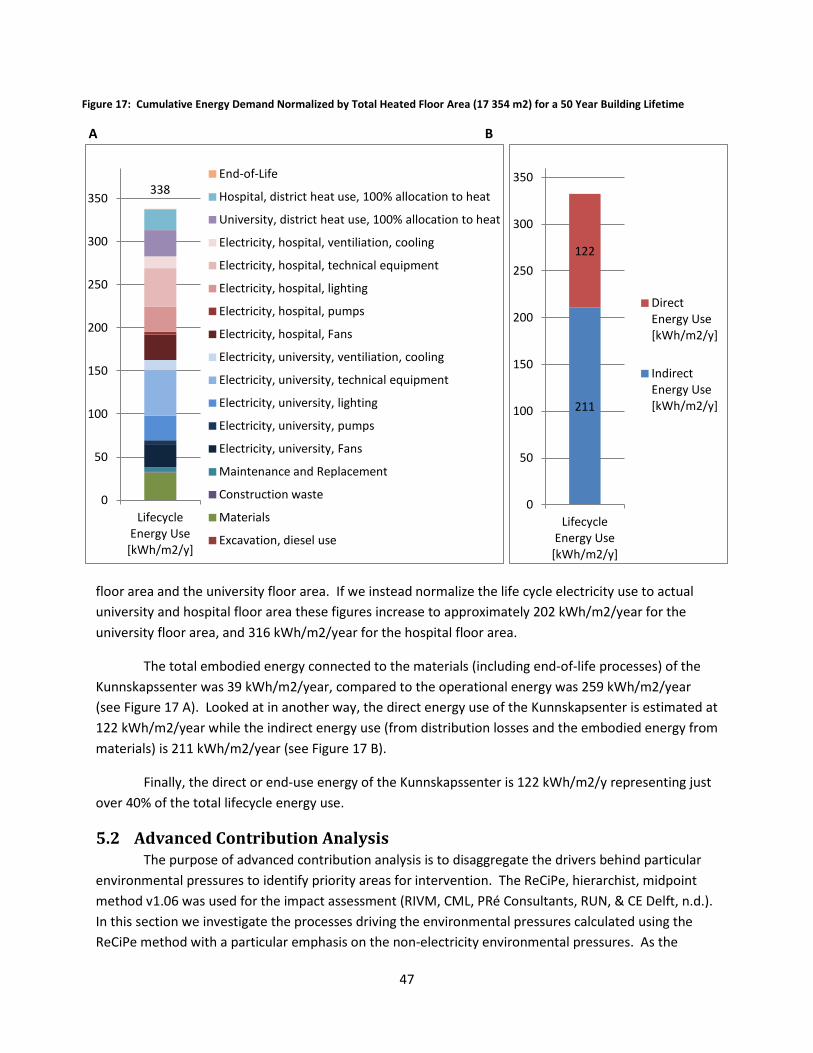
47

floor area and the university floor area. If we instead normalize the life cycle electricity use to actual university and hospital floor area these figures increase to approximately 202 kWh/m2/year for the university floor area, and 316 kWh/m2/year for the hospital floor area.

The total embodied energy connected to the materials (including end-of-life processes) of the Kunnskapssenter was 39 kWh/m2/year, compared to the operational energy was 259 kWh/m2/year (see Figure 17 A). Looked at in another way, the direct energy use of the Kunnskapsenter is estimated at 122 kWh/m2/year while the indirect energy use (from distribution losses and the embodied energy from materials) is 211 kWh/m2/year (see Figure 17 B).

Finally, the direct or end-use energy of the Kunnskapssenter is 122 kWh/m2/y representing just over 40% of the total lifecycle energy use.

5.2 Advanced Contribution Analysis The purpose of advanced contribution analysis is to disaggregate the drivers behind particular

environmental pressures to identify priority areas for intervention. The ReCiPe, hierarchist, midpoint method v1.06 was used for the impact assessment (RIVM, CML, PRé Consultants, RUN, & CE Delft, n.d.). In this section we investigate the processes driving the environmental pressures calculated using the ReCiPe method with a particular emphasis on the non-electricity environmental pressures. As the

Figure 17: Cumulative Energy Demand Normalized by Total Heated Floor Area (17 354 m2) for a 50 Year Building Lifetime

A B

338

0

50

100

150

200

250

300

0

50

100

150

200

250

300

350

Lifecycle Energy Use

[kWh/m2/y]

End-of-Life

Hospital, district heat use, 100% allocation to heat

University, district heat use, 100% allocation to heat

Electricity, hospital, ventiliation, cooling

Electricity, hospital, technical equipment

Electricity, hospital, lighting

Electricity, hospital, pumps

Electricity, hospital, Fans

Electricity, university, ventiliation, cooling

Electricity, university, technical equipment

Electricity, university, lighting

Electricity, university, pumps

Electricity, university, Fans

Maintenance and Replacement

Construction waste

Materials

Excavation, diesel use

211

122

0

50

100

150

200

250

300

350

Lifecycle Energy Use

[kWh/m2/y]

Direct Energy Use [kWh/m2/y]

Indirect Energy Use [kWh/m2/y]

48

results were undertaken using the NORDEL electricity mix from ecoinvent v2.2, the electricity based emissions can be easily replicated by curious readers. To help guide the investigation on particular environmental pressures, the results from the ReCiPe v1.06 method are normalized to per capita European emissions.

Compared to the primary energy assessment in the previous section, materials generally play a significantly larger role in environmental pressures (see Figure 18).17 However, we see that electricity use still plays a dominant role representing more than 50% of the contribution for 12 of the 18 impact categories. Only for agricultural land occupation and urban land occupation are the contributions from electricity less than 40%.

Materials, including construction waste as well as maintenance and replacement activities, contribute more than 25% of total environmental pressures in 13 of 18 impact categories and contribute more than 30% of total pressures in 8 of the 18 impact categories. While materials represent over 50% of the pressure for the indicators agricultural and urban land occupation, it is determined in the analysis below that the total value for land occupation is small when normalized to per capita European land occupation.

District heating on the other hand is a substantial driver for pressures on freshwater and marine ecotoxicity representing 37% and 33% respectively of the total impacts on these categories. Other important indicators impacted by district heating include climate change (16%), human toxicity (16%), photochemical oxidant formation (11%), marine eutrophication (11%) and fossil depletion (8%).

End-of-Life processes, remembering that this excludes the emissions due to waste incineration which are allocated 100% to the heat produced from waste incineration, play a minor role in photochemical oxidant formation (4%), and particulate matter formation (8%).

By normalizing the total non-electricity emissions to per capita European and Global emissions from 2000 using data contained within SimaPro (Sleeswijk, van Oers, Guinée, Struijs, & Huijbregts, 2008) we get a better picture of the scale of emissions in different impact categories and highlight the impact categories that should be the emphasis of further investigation (see Figure 19 A and B). One peculiarity seen from these normalizations is the stark difference for the indicator natural land transformation. While it is very high when normalized to European levels representing the yearly pressure from almost 15 000 Europeans, the normalization to global levels represents the yearly pressure of less than 200 individuals. The reason for this may be that production activities within Europe are not as land intensive due to the service orientated nature of their economies compared to the world as a whole.

In the analysis below, we take a more detailed look at the non-electricity drivers for 7 impact categories: climate change, particulate matter formation and terrestrial acidification for their global importance as well as human toxicity, freshwater eutrophication, freshwater ecotoxicity and marine ecotoxicity because of the high normalized contribution based on Figure 19 A and B.

17 The data for figure 5.2 can be found in tabular form in Appendix G

49

Figure 18: Advanced Contribution Analysis of Using ReCiPe, Midpoint, Hierarchist Method. Impacts Expressed per Unit Floor Area per Year for a 50 Year Building Lifetime

7,70E+00 3,86E+00 4,01E-01 5,43E-03 2,83E-01 8,11E+00 3,25E-01 3,12E-01 2,25E-02 5,15E-03 9,25E-03 9,99E-02 3,65E+01 5,66E-02 8,50E-02 1,94E+01 2,12E-06 3,36E+01

0 % 10 % 20 % 30 % 40 % 50 % 60 % 70 % 80 % 90 % 100 %

0 % 20 % 40 % 60 % 80 % 100 %

Fossil depletion [kg oil eq/m2/y] Metal depletion [kg Fe eq/m2/y]

Water depletion [m3/m2/y] Natural land transformation [m2/m2/y]

Urban land occupation [m2a/m2/y] Agricultural land occupation [m2a/m2/y]

Marine ecotoxicity [kg 1,4-DB eq/m2/y] Freshwater ecotoxicity [kg 1,4-DB eq/m2/y] Terrestrial ecotoxicity [kg 1,4-DB eq/m2/y]

Marine eutrophication [kg N eq/m2/y] Freshwater eutrophication [kg P eq/m2/y] Terrestrial acidification [kg SO2 eq/m2/y]

Ionising radiation [kg U235 eq/m2/y] Particulate matter formation [kg PM10 eq/m2/y]

Photochemical oxidant formation [kg NMVOC/m2/y] Human toxicity [kg 1,4-DB eq/m2/y]

Ozone depletion [kg CFC-11 eq/m2/y] Climate change [kg CO2 eq/m2/y]

50

Figure 19: Non-Electricity Lifecycle Emissions from Kunnskapssenter Normalized to A) Per Capita European Emissions, and B) Per Capita Global Emissions.

A)

B)

0

10000

20000

30000

40000

50000

60000

70000

End-of-Life

District Heating

Maintenance and Replacement Construction waste

Excavation

Materials

0

10000

20000

30000

40000

50000

60000

70000

End-of-Life

District Heating

Maintenance and Replacement Construction waste

Excavation

Materials

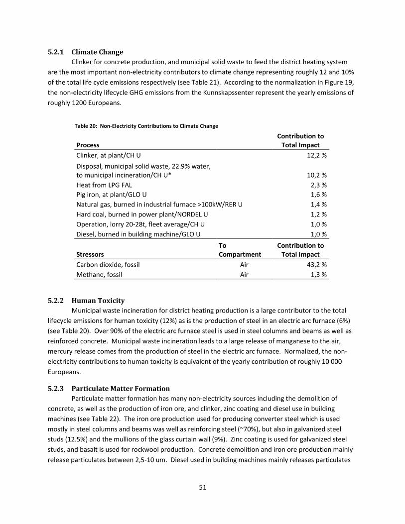
51

5.2.1 Climate Change Clinker for concrete production, and municipal solid waste to feed the district heating system

are the most important non-electricity contributors to climate change representing roughly 12 and 10% of the total life cycle emissions respectively (see Table 21). According to the normalization in Figure 19, the non-electricity lifecycle GHG emissions from the Kunnskapssenter represent the yearly emissions of roughly 1200 Europeans.

5.2.2 Human Toxicity Municipal waste incineration for district heating production is a large contributor to the total

lifecycle emissions for human toxicity (12%) as is the production of steel in an electric arc furnace (6%) (see Table 20). Over 90% of the electric arc furnace steel is used in steel columns and beams as well as reinforced concrete. Municipal waste incineration leads to a large release of manganese to the air, mercury release comes from the production of steel in the electric arc furnace. Normalized, the non-electricity contributions to human toxicity is equivalent of the yearly contribution of roughly 10 000 Europeans.

5.2.3 Particulate Matter Formation Particulate matter formation has many non-electricity sources including the demolition of

concrete, as well as the production of iron ore, and clinker, zinc coating and diesel use in building machines (see Table 22). The iron ore production used for producing converter steel which is used mostly in steel columns and beams was well as reinforcing steel (~70%), but also in galvanized steel studs (12.5%) and the mullions of the glass curtain wall (9%). Zinc coating is used for galvanized steel studs, and basalt is used for rockwool production. Concrete demolition and iron ore production mainly release particulates between 2,5-10 um. Diesel used in building machines mainly releases particulates

Table 20: Non-Electricity Contributions to Climate Change

Process Contribution to

Total Impact Clinker, at plant/CH U 12,2 % Disposal, municipal solid waste, 22.9% water, to municipal incineration/CH U* 10,2 % Heat from LPG FAL 2,3 % Pig iron, at plant/GLO U 1,6 % Natural gas, burned in industrial furnace >100kW/RER U 1,4 % Hard coal, burned in power plant/NORDEL U 1,2 % Operation, lorry 20-28t, fleet average/CH U 1,0 % Diesel, burned in building machine/GLO U 1,0 %

Stressors To Compartment

Contribution to Total Impact

Carbon dioxide, fossil Air 43,2 % Methane, fossil Air 1,3 %

52

Table 21: Non-Electricity Contributions to Human Toxicity

Process Contribution to

Total Impact Disposal, municipal solid waste, 22.9% water, to municipal incineration/CH U* 12,0 % Steel, electric, un- and low-alloyed, at plant/RER U - NORDEL 6,8 % Disposal, sulfidic tailings, off-site/GLO U 2,4 % Disposal, spoil from coal mining, in surface landfill/GLO U 1,9 % Disposal, spoil from lignite mining, in surface landfill/GLO U 1,6 % Heat from LPG FAL 1,3 %

Stressors To Compartment Contribution to

Total Impact Manganese Water 12,0 % Mercury Air 7,6 % Lead Water 2,5 % Barium Water 2,4 % Arsenic, ion Water 2,4 % Lead Air 2,3 %

Table 22: Non-Electricity Contributions to Particulate Matter Formation

Process Contribution to

Total Impact Disposal, building, concrete, not reinforced, to recycling/CH U 6,3 % Iron ore, 46% Fe, at mine/GLO U 4,5 % Clinker, at plant/CH U 3,0 % Zinc coating, coils/RER U - NORDEL 2,9 % Diesel, burned in building machine/GLO U 2,7 % Ceramic tiles, at regional storage/CH U 1,9 % Basalt, at mine/RER U 1,7 % Operation, lorry 20-28t, fleet average/CH U 1,7 % Electricity, at cogen ORC 1400kWth, wood, allocation exergy/CH U 1,2 % Bauxite, at mine/GLO U 1,1 % Process-specific burdens, municipal waste incineration/CH U 1,0 %

Stressors To Compartment

Contribution to Total Impact

Particulates, > 2.5 um, and < 10um Air 15,7 % Nitrogen oxides Air 13,0 % Particulates, < 2.5 um Air 10,3 % Sulfur dioxide Air 6,0 % Ammonia Air 2,4 %

53

less than 1.5 um, and clinker is the source of nitrogen oxides and sulfur dioxide. Zinc coating mainly releases ammonia, and particulates between 2,5-10 um.

5.2.4 Terrestrial Acidification The main non-electricity sources of terrestrial acidification include zinc coating, clinker, and

diesel consumed in building machines (see Table 23). As discussed above, zinc coating releases ammonia, while clinker releases nitrogen oxides, sulfur dioxide and ammonia. Diesel used in building machines used mainly for the demolition of reinforced concrete products leads to the release of nitrogen oxides, sulfur dioxide and ammonia.

Table 23: Non-Electricity Contributions to Terrestrial Acidification

Process Contribution to

Total Impact Zinc coating, coils/RER U - NORDEL 8,5 % Clinker, at plant/CH U 5,0 % Diesel, burned in building machine/GLO U 2,8 % Operation, lorry 20-28t, fleet average/CH U 2,1 % Flat glass, uncoated, at plant/RER U 1,8 % Operation, transoceanic freight ship/OCE U 1,6 % Process-specific burdens, municipal waste incineration/CH U 1,4 % LPG FAL 1,1 % Sinter, iron, at plant/GLO U 1,0 %

Stressors To Compartment Contribution to

Total Impact Nitrogen oxides Air 18,6 % Sulfur dioxide Air 16,9 % Ammonia Air 10,3 % Sulfur oxides Air 1,1 %

Table 24: Non-Electricity Contributions to Freshwater Eutrophication

Process Contribution

to Total Impact Disposal, spoil from coal mining, in surface landfill/GLO U 6,9 % Disposal, spoil from lignite mining, in surface landfill/GLO U 5,9 % Fertilizer-P I 4,3 % Disposal, sulfidic tailings, off-site/GLO U 3,1 % Disposal, municipal solid waste, 22.9% water, to municipal incineration/CH U* 2,7 % Disposal, basic oxygen furnace wastes, 0% water, to residual material landfill/CH U 1,9 % Disposal, spoil from coal mining, in surface landfill/GLO U 1,7 %

Stressors To Compartment

Contribution to Total Impact

Phosphate Water 30,0 %

54

5.2.5 Freshwater Eutrophication Freshwater eutrophication is largely a result of coal and lignite mining processes. Lignite is used

in the production of pig iron and European (UCTE) electricity respectively. The UCTE electricity in turn is used in a wide range of upstream processes including the krypton gas used in triple glazed windows, clinker, pig iron for converter steel, liquid oxygen for electric arc furnace steel, and sodium hydroxide for municipal waste incineration. Coal is used mainly for producing pig iron, but also clinker, UCTE electricity, and rockwool. The fertilizer, on the other hand, is a direct input into linseed production which is used for linoleum flooring. The normalized freshwater eutrophication emissions is relatively large representing the yearly emissions of roughly 3800 Europeans.

5.2.6 Freshwater Ecotoxicity As we saw in the contribution analysis displayed in Figure 18, the district heating system was an

important contributor to both freshwater and marine ecotoxicity. This is driven by municipal solid waste incineration as a result of emissions of nickel and zinc ions as well as manganese (see Table 26). Slag disposal from electric arc furnaces contributes vanadium and nickel ions. Finally, disposal processes for coal and lignite which, as mentioned above, are required upstream in the supply chain network, both contribute Nickel ion and Manganese. Normalized, the non-electricity freshwater ecotoxicity emissions represent the emissions of over 14 000 Europeans per year.

5.2.7 Marine Ecotoxicity The drivers of marine ecotoxicity parallel those of freshwater ecotoxicity with district heating

through municipal solid waste incineration being the major contributor followed by slag from steel production using an electric arc furnace, along with coal mining, driving by pig iron production, and

Table 25: Non-Electricity Contributions to Freshwater Ecotoxicity

Process Contribution to

Total Impact Disposal, municipal solid waste, 22.9% water, to municipal incineration/CH U* 35,5 % Disposal, slag, unalloyed electr. steel, 0% water, to residual material landfill/CH U 4,7 % Disposal, spoil from coal mining, in surface landfill/GLO U 2,6 % Disposal, spoil from lignite mining, in surface landfill/GLO U 2,2 % Disposal, nickel smelter slag, 0% water, to residual material landfill/CH U 2,0 % Disposal, sludge from steel rolling, 20% water, to residual material landfill/CH U 1,8 % Disposal, sulfidic tailings, off-site/GLO U 1,8 % Disposal, redmud from bauxite digestion, 0% water, to residual material landfill/CH U 1,6 %

Stressors To Compartment Contribution to

Total Impact Nickel, ion Water 33,8 % Zinc, ion Water 7,4 % Vanadium, ion Water 5,4 % Manganese Water 4,7 % Bromine Water 1,5 %

55

lignite mining waste (see Table 25). The normalized value for marine ecotoxicity is the highest of all impact categories representing the yearly emissions of roughly 18 000 Europeans.

5.3 Sensitivity Analysis The sensitivity analysis evaluates the influence of five key parameters on the results from the

reference scenario for the seven key indicator categories presented in the previous section. The five key parameters include the building lifetime, the fraction of construction waste, the electricity mix, the recycled content of reinforcing steel, and the allocation of emissions from waste incineration. As a starting point, the assumed values for these five key parameters in the reference scenario are outlined (see Table 27).

The building lifetime for the reference scenario is 50 years. It is interesting to note that the demolition report for the hospital complex (høyblokka) that was demolished to make room for the Kunnskapssenter states a construction year for the buildings ranging of 1957-1990. The reference scenario assumed 5% construction waste.

Table 26: Non-Electricity Contributions to Marine Ecotoxicity

Process Contribution to

Total Impact Disposal, municipal solid waste, 22.9% water, to municipal incineration/CH U* 31,3 % Disposal, slag, unalloyed electr. steel, 0% water, to residual material landfill/CH U 4,4 % Disposal, spoil from coal mining, in surface landfill/GLO U 2,4 % Disposal, spoil from lignite mining, in surface landfill/GLO U 2,0 % Disposal, nickel smelter slag, 0% water, to residual material landfill/CH U 1,9 % Disposal, sludge from steel rolling, 20% water, to residual material landfill/CH U 1,7 % Disposal, sulfidic tailings, off-site/GLO U 1,6 % Disposal, redmud from bauxite digestion, 0% water, to residual material landfill/CH U 1,5 %

Stressors To Compartment Contribution to

Total Impact Nickel, ion Water 31,6 % Zinc, ion Water 6,0 % Vanadium, ion Water 5,1 % Manganese Water 4,3 %

Table 27: Parameters Assessed for Sensitivity Analysis

Parameter Reference Scenario Alternative Scenario(s) Building lifetime 50 years 30, 60, and 75 years Construction Waste 5 % 10 % Electricity mix Nordic (NORDEL) European (UCTE)

Reinforcing steel mix -Steel, converter, unalloyed (27%) -Steel, electric, un- and low-alloyed (73%)

-Steel, converter, unalloyed (63%) -Steel, electric, un- and low-alloyed (37%)

Emissions allocation from waste incineration

100 % to Heat production 100% to Waste function

56

Figure 20: Sensitivity Analysis – Relative change from Reference Scenario for Seven Impact Categories

637,42 %

0,00 %

50,00 %

100,00 %

150,00 %

200,00 %

250,00 %

300,00 %

350,00 %

30y

10%

CW

Re

fere

nce

UCT

E el

mix

EU

stee

l mix

10

0% W

A 60

y 75

y 30

y 10

% C

W

Refe

renc

e U

CTE

el m

ix

EU st

eel m

ix

100%

WA

60y

75y

30y

10%

CW

Re

fere

nce

UCT

E el

mix

EU

stee

l mix

10

0% W

A 60

y 75

y 30

y 10

% C

W

Refe

renc

e U

CTE

el m

ix

EU st

eel m

ix

100%

WA

60y

75y

30y

10%

CW

Re

fere

nce

UCT

E el

mix

EU

stee

l mix

10

0% W

A 60

y 75

y 30

y 10

% C

W

Refe

renc

e U

CTE

el m

ix

EU st

eel m

ix

100%

WA

60y

75y

30y

10%

CW

Re

fere

nce

UCT

E el

mix

EU

stee

l mix

10

0% W

A 60

y 75

y

Climate change Human toxicity Particulate matter formation

Terrestrial acidification Freshwater eutrophication

Freshwater ecotoxicity Marine ecotoxicity

30y = 30 year building lifetime 10% CW = 10% construction waste Reference = reference scenario UCTE el mix = European electricity mix EU steel mix = European reinforcing steel mix (ecoinvent) 100% WA = 100% emissions allocation to waste incineration 60y = 60 year building lifetime 75y = 75 year building lifetime

57

The electricity supply directly consumed during the building operation as well as the electricity for the district heating system and the indirect electricity used for a subset of building materials (refer back to section 3.3.4) is a Nordic mix (NORDEL) from ecoinvent v2.2. For reinforcing steel, the input ratio between converter steel and electric steel was altered – from what is referred to as the European steel mix in one scenario below, the default mix in ecoinvent v2.2 – to a ratio consistent with the recycled content ratio for Norwegian reinforcing steel products.18 Finally, the emissions from municipal waste incineration were allocated 100% to the production of heat and the disposal of municipal waste appears emissions free in the results.

As we see from Figure 20, the electricity mix has the strongest influence on the results via electricity consumption during the use phase. The increase in emissions from the reference scenario for the UCTE scenario ranges from 173% for particulate matter formation, to over 600% for freshwater eutrophication. Interestingly, the impact on materials from a change in the electricity mix is relatively unchanged compared to the reference scenario throughout the impact categories. From the analysis in the previous section, however, we saw that many of the material based emissions were not electricity related. Process emissions from clinker production, for example, being the main material driver for climate change. Direct emissions from the demolition of concrete were the main driver for the formation of particulate matter on the materials side. The influence of electricity indirectly through materials is slightly more pronounced in the category freshwater eutrophication where we saw a dramatic increase in the pressure from the European electricity mix compared to the Nordic electricity mix.

Not surprisingly, we also see that the building lifetime has a notable influence on the results which is overwhelmingly due to a greater increase in electricity during a longer, or shorter, use phase.

Increasing the construction waste of bulk materials delivered to the building site from 5% in the reference scenario to 10% had little effect on the overall results due to the small relative contribution of building materials.

Change the recycled steel content had a small increases in freshwater eutrophication (5%) and on particulate matter formation (4%), while slightly decreasing Human toxicity (-2%).

Finally, shifting the allocation for municipal waste incineration from heat production to waste disposal lead to a decrease in all impact categories previously associated with district heating including climate change, human toxicity, freshwater ecotoxicity, and marine ecotoxicity. The reason for this is simply that waste disposal during the use phase of the building was not inventoried.

18 Refer back to section 3.3.6 in the methodology section for a full explanation.

58

6 Discussion It can be challenging to contextualize LCA results. To help address this, the discussion below compares the results from the Kunnskapssenter with building LCAs from the literature. In addition an emphasis is put on the results for climate change by sketching out a one tonne per capita GHG emissions scenario through 2050 to consider how the Kunnskapssenter will impinge on the carbon budget of its employees in a carbon constrained world.

The reference scenario described above suggests lifecycle emissions of just over 29 Mt of CO2-equivalents for the Kunnskapssenter. This boils down to almost 0.6 Mt/yr. While staffing numbers for the Kunnskapssenter were not available, data from the University Hospital of South Manchester (UHSM) include a staff of 5800 individuals for the 130 000 m2 complex or almost 22.5 m2 per staff member. As a comparison, the floor area per employee of other building types is presented in Figure 21.

Applying floor area per employee ratio of the UHSM to the heated floor area of the Kunnskapssenter suggests a staff of approximately 775 individuals.19 Normalizing the total yearly emissions to the estimated staff population leads to an emissions total of roughly 0.75 tonnes CO2-eq

19 The floor are for the Kunnskapssenter refers to heated floor area which includes technical rooms. It is not clear if the UHSM floor area refers to heated floor area or gross floor area.

Figure 21: Floor Area per Employee

UHSM = University Hospital South Manchester Sources: (Ashden, 2012; Drivers Jonas Deloitte, 2010) NB: data for UHSM is reported as staff per floor area, which may include part-time staff, whereas the rest of the data from the UK’s Employment Density Guide is reported in floor area per fulltime equivalents

0

10

20

30

40

50

60

70

80

UHSM Industrial Warehouse & Distribution

Office Data Centres Food Superstore

Restaurants

59

per employee per year. Compared to per capita emission in Norway of roughly 10.7 tonnes20 CO2-eq in 2011, the yearly emissions of the Kunnskapssenter normalized to a rough estimate of total staff seems relatively minor. Using emissions factors for Norwegian electricity rather than Nordic electricity would have made the ghg emissions even smaller – perhaps just under half the total in this estimate.

Compared to the recent carbon footprint results from Larsen et al. (2011) for the Norwegian University of Science and Technology, these figures are quite low – and for a reason. Using a hybrid LCA methodology to capture the carbon footprint of university expenditures, their results suggest roughly 16.7 tonnes CO2-eq per employee or 4.6 tonnes of CO2-eq per student. The system boundaries using an expenditure based approach make the overall results difficult to compare to the current study, but demonstrate the importance of items like travel, equipment and consumables. However, they find that the construction and maintenance of buildings are responsible for 19% of the carbon footprint of the university or roughly 3.2 tonnes per employee per year, while the energy use (electricity, district heating, heating oil) is also responsible for 3.2 tonnes per employee per year. A complete breakdown of the results from Larsen et al (2011) are displayed in Figure 22.

Given the proportion of space dedicated to classrooms libraries and laboratories, we should expect the floor space per university employee to be comparatively high. In fact given a net floor area of 705 000 m2 and a gross floor area of 800 000 m2 for NTNU21 along with roughly 20 000 employees assumed by Larsen et al. (2011), the actual floor area per employee is 35-40 m2 depending on the

20 Per capita GHG emissions in Norway are roughly 10.7 tonnes, based on a population of 4.92 million in 2011 and total domestic emissions of 52.7 Mt in 2011 (Statistics Norway, 2011, 2012). 21 Thanks to Arne Rønning for providing this data.

Figure 22: Carbon Footprint of NTNU

Source: (Larsen, Pettersen, Solli, & Hertwich, 2011)

60

metric used. In addition, with an average energy consumption of NTNU’s building stock of 290 kWh/m222 in 2010 compared to the 122 kWh/m2 for the Kunnskapssenter, the difference between the carbon footprint per university employee estimated by Larsen et al. (2011) and the carbon footprint per hospital employee from this assessment is not so surprising.

In a carbon constrained future however, what does 0.75 tonnes CO2-eq actually mean? Allowing for emissions trading, the German Advisory Council on Global Change (2009) argues that per capita carbon budgets (considering only CO2) for current high emitting countries, which are defined as emitting more that 5.4 tonnes per capita per year, should be below 1 tonne per capita per year by 2050 (see Figure 23). While the results from this thesis consider CO2-eqs and thus consider more GHGs than just CO2, CO2 remains the major GHG representing over 84% of Norways GHG emissions in 2011 (Statistics Norway, 2012).

As the scope of this study was limited to the construction and operation of the Kunnskassenter and did not consider technical equipment, consumables, commuter traffic and business travel of the

22 Thanks to Geir Skaaren for providing this data.

Figure 23: Per Capita Emissions Budget for CO2 with and without Emissions Trading

Based on CO2 emissions from 2008, group 1 emissions (>5.4 tonnes per capita per year), group 2 countries (2.7-5.4 tonnes per capita per year), group 3 (<2.7 tonnes) Source: (German Advisory Council on Global Change, 2009)

61

employees, the 0.75 tonnes CO2-eq appears rather high. While it is clear that decarbonisation of the energy system is imperative, it was also found that clinker production was responsible for about 12% of overall GHG emissions. This suggests that just the concrete in the building used by these employees represents roughly 10% of their carbon budget. This is important because the GHG emissions from clinker production are predominantly from the chemical reactions in the process rather than from the energy supply. 10% seems like a rather high proportion of an individuals carbon budget given that the analysis is based on a Nordic electricity mix which has a relatively low carbon budget.

While it is clear that decarbonisation of the energy system is critical, this study also raises the question as to what extent we can continue to build concrete intensive buildings.

As atmospheric measurements for CO2 emissions pass 400 parts per million for the first time in several Arctic regions (Levin, 2012), we are reminded of the pressing nature of understanding the drivers for carbon footprints through a lifecycle perspective.

62

7 Limitations and Future Work While the implementation of BIM is set to transform the information available to building

managers, it also signals an opportunity for establishing a deeper understanding of the material requirements for our building stock through detailed bottom up assessments. With the implementation of any new technology however, there are inevitably a few road bumps that can limit the application.

Three basic limitations for this work are due to inherent uncertainty in the BIM, product supplier uncertainty, and the incomplete construction of the building.

Uncertainty in the BIM model has four distinct sources. First, several composite objects are modeled as a solid objects in the BIM model. This is the case for many types of walls whether it is a reinforced concrete wall or an insulated wall with steel or wood studs, drywall, wind barrier, etc. Establishing the material composition of these objects relies on architectural drawings and other literature sources. A second challenge is the human error in BIM modelling. A particular wall with a material tag indicating the structural material was composed of wooden studs in the BIM model, for example, was found to be reinforced concrete upon a site visit. A final problem associated with relying on BIM is that it provides volume estimates which need to be turned into units of mass or area so that they are consistent with functional units in SimaPro. The material densities applied in this analysis have been taken from generic sources and adds additional uncertainty into the model. A final and rather significant issue with the BIM model was due to discrepancies discovered between certain volume estimates in the quantity take-off and the measured volume of the objects in the BIM model. It first became clear when the results from aluminum cladding seemed disproportionately large. Upon further investigation, it was discovered that the volume of a few of the aluminum cladding objects were exported in the quantity take-off were 10-30x larger then the measured dimensions from within the BIM model and manual measurements were required to obtain more accurate results. While an attempt was made to clarify this issue with the BIM modeller for the project, Pål Ingdal, this issue is still un-resolved and should be clarified in future work. It is unclear if this was an isolated issue or something more systemic.

Another limitation involves the transport distances associated with various building products. Since the actual supplier for various products was not known, an attempt was made to establish an inventory of regional producers available to supply the Trondheim market. Given that the purchase of building products is driven by factors such as price and product specifications (e.g. design, quality, functionality, eco-labels, etc.) it is not necessarily correct to assume that purchases are driven by the availability of local suppliers except for the instances where transport distances are highly correlated to price and there is little variation in product quality amongst suppliers such as with concrete.

Building energy modelling is a difficult task due to the human, rather then strictly technical nature of task. Building inhabitants that do not understand the low energy design features of a building or are gluttonous in their consumption are bound to confound the results of even the best energy modellers. Because the Kunnskapssenter has not yet been completed, the outcomes of this LCA relies

63

on the energy modelling data produced in the planning stages of the project and is thus subject to a certain uncertainty. It would be interesting to monitor the results of actual energy consumption in the future to update the results presented here.

Given the limited data on the material composition of health care infrastructure in the literature, the results of this LCA could provide a useful contribution towards investigating the lifecycle impacts of health care services in addition to the contribution that healthcare infrastructure has on the environmental pressures of urban development, especially in rapidly developing countries like China and India as.

64

8 Conclusion In concluding, this thesis presents an original contribution to the literature on building LCA due

to the lack of building LCA’s for hospital buildings, and the innovative low-energy design standards of the building which allows for a bettering understanding of the trade-offs between different stages of the building lifecycle.

While the lifecycle energy consumption, which was 333 kWh/m2/year over a 50 year building lifecycle, was found to be relatively low compared to results for office buildings presented in the literature, this is rather significant given the energy intensity of hospital buildings compared to office buildings.

While energy-use from the operation of the building was still the largest phase for most indicators of environmental performance, non-energy phases were far from trivial. Roughly 30% of GHG emissions, 43% of particulate matter formation, and 41% of terrestrial acidification pressure was a results of non-energy phases of the building lifecycle. Notably these results were observed with 100% of the emissions from waste incineration allocated to heat production.

65

Literature Cited Adalberth, K. (1997). Energy use during the life cycle of single-unit dwellings: Examples. Building and

Environment, 32(4), 321–329. doi:10.1016/S0360-1323(96)00069-8

Adalberth, K., Almgren, A., & Petersen, E. H. (2001). Life cycle assessment of four multi-family buildings.

International Journal of Low Energy and Sustainable Buildings, 2, 1–21.

Anderson, J., Shiers, D., & Sinclair, M. (2002). The green guide to specification: an environmental

profiling system for building materials and components. Oxford, UK: Blackwell Publishing.

Ashden. (2012). Case study summary: University hospital of South Manchester NHS Foundation Trust.

Retrieved from http://www.ashden.org/

Autodesk. (2012, March 6). Autodesk Revit Architecture. Autodesk. Retrieved March 6, 2012, from

http://usa.autodesk.com/adsk/servlet/pc/index?id=17801984&siteID=123112&s_tnt=31959:0:0

Benjamin Moore. (2012). Paint calculator. Benjamin Moore. Paint retailer. Retrieved May 25, 2012,

from http://www.benjaminmoore.com/en-ca/for-your-home/paint-

calculator;jsessionid=S9hjP1dSyCWHQFmKVjx7p0LB5LK2kSVn6qWcqhhRQkXlrnGtsP1T!-

694302269!NONE

Bilec, M. M., Ries, R. J., & Matthews, H. S. (2010). Life-Cycle Assessment Modeling of Construction

Processes for Buildings. Journal of Infrastructure Systems, 16(3), 199.

doi:10.1061/(ASCE)IS.1943-555X.0000022

Blengini, G.A. (2006). Life cycle assessment tools for sustainable development: case studies for the

mining and construction industries in Italy and Portugal (PhD Dissertation). Instituto Superior

Tecnico, Technical University of Lisbon, Lisbon, Portugal.

Blengini, Gian Andrea, & Garbarino, E. (2010). Resources and waste management in Turin (Italy): the

role of recycled aggregates in the sustainable supply mix. Journal of Cleaner Production, 18(10-

11), 1021–1030. doi:10.1016/j.jclepro.2010.01.027

66

Brattebø, H., & Reenaas, M. (2012). Comparing CO2 and NOX emissions from a district heating system

with mass-burn waste incineration versus likely alternative solutions – City of Trondheim, 1986–

2009. Resources, Conservation and Recycling, 60, 147–158. doi:10.1016/j.resconrec.2011.11.001

Canadian Plywood Association. (n.d.). Plywood engineering properties: physical properties. CANPLY:

Canadian Plywood. Retrieved May 1, 2012, from

http://www.canply.org/english/products/comparison/comparison_all.htm

Canadian Sheet Steel Building Institute. (2006, May). Sheet steel gauges and thickness. Retrieved from

http://www.cssbi.ca/

Coelho, A., & de Brito, J. (2012). Influence of construction and demolition waste management on the

environmental impact of buildings. Waste Management, 32(3), 532–541.

doi:10.1016/j.wasman.2011.11.011

Con-Form AS. (2010). Veggelement. The Norwegian EPD Foundation. Retrieved from http://www.epd-

norge.no

Contiga AS. (2007, August). Steel structures of HSQ, ISQ and HSK sections. The Norwegian EPD

Foundation. Retrieved from http://www.epd-norge.no

Contiga AS. (2008). Veggelement uten isolasjon. The Norwegian EPD Foundation. Retrieved from

http://www.epd-norge.no/getfile.php/PDF/EPD/Byggevarer/NEPD128N%20Contiga.pdf

Contiga AS. (2009a). Søyle. The Norwegian EPD Foundation. Retrieved from http://www.epd-

norge.no/getfile.php/PDF/EPD/Byggevarer/NEPD127N%20Contiga.pdf

Contiga AS. (2009b). Bjelke. The Norwegian EPD Foundation. Retrieved from http://www.epd-norge.no/

Corrostop. (2009, April 15). Exterior alkyd paint for metal surfaces. Retrieved from

http://questionpeinture.com/files/pdf/en/MetalmasterHammered_en.pdf

Cowi AS. (2009, September 14). Energinotat.

67

Cuéllar-Franca, R. M., & Azapagic, A. (2012). Environmental impacts of the UK residential sector: Life

cycle assessment of houses. Building and Environment, 54, 86–99.

doi:10.1016/j.buildenv.2012.02.005

Dahlstrøm, O. (2010). Life-cycle assessment of the building envelope elements of a wood-based passive

house: Modern highly effective windows. The Norwegian University of Science and Technology,

Trondheim, Norway. Retrieved from

http://www.klimatre.no/uploads/KlimaTre/Publikasjoner/Project_Fall_2010_Dahlstrom.pdf

Doka, G. (2009). Life cycle inventory of waste treatment services ( No. No. 13). Dubendorf, CH: Swiss

Centre for Life Cycle Inventories. Retrieved from www.ecoinvent.org

Drivers Jonas Deloitte. (2010). Employment densities guide. Office of Project and Programme Advice and

Training, Homes and Communities Agency. Retrieved from

http://www.homesandcommunities.co.uk/

Dupont. (2012). Tyvek® Housewrap - Vapour permeable membrane. Dupont. Building Product

Manufactuer. Retrieved May 2, 2012, from

http://www2.dupont.com/Tyvek_Construction/en_IE/products/wall_products/housewrap.html

ecoinvent Centre. (2010). ecoinvent data v2.2. Retrieved May 13, 2012, from

http://www.ecoinvent.org/

Ecos Organic Paints. (n.d.). Paint calculator. Retrieved June 4, 2012, from

http://www.ecosorganicpaints.co.uk/paint-calculator/

Euroclad. (n.d.). Zinc roofing systems. Euroclad: Architectural Wall Cladding and Roofing. Industry.

Retrieved May 24, 2012, from http://www.euroclad.com.au/standing-seam-zinc-roofing.html

European Commission - Joint Research Centre - Institute for Environment and Sustainability. (2010).

International reference life cycle data system (ILCD) handbook - General guide for life cycle

assessment - Detailed guidance ( No. First edition EUR 24708 EN). Luxembourg: Publications

68

Office of the European Union. Retrieved from

http://lct.jrc.ec.europa.eu/assessment/assessment/projects

Everbright LECA Co., Ltd. (n.d.). Company introduction. Everbright LECA Co., Ltd. Building Product

Manufactuer. Retrieved May 13, 2012, from http://www.leca.cc/

Gerflor. (n.d.). Healthcare floor covering. Industry website. Retrieved June 4, 2012, from

http://www.gerflor.com/int/floors-for-

professionals/sante/environnement1/environnement113.html

German Advisory Council on Global Change. (2009). Solving the climate dilemma: The budget approach.

Berlin. Retrieved from http://www.wbgu.de/en/special-reports/sr-2009-budget-approach/

German Advisory Council on the Environment. (2011). Pathways towards a 100 % renewable electricity

system (p. 434). Retrieved from

http://www.umweltrat.de/SharedDocs/Downloads/EN/02_Special_Reports/2011_10_Special_R

eport_Pathways_renewables.html

Gipsplate. (n.d.).Wikipedia. Retrieved from http://no.wikipedia.org/wiki/Gipsplate

Gjerlow, J. A. (2011). Gyproc, Plasterboard 12.5 mm, GN13 (Environmental Product Declaration No.

NEPD NO: 223E). EPD Norge. Retrieved from www.epd-norge.no

Glass for Europe. (n.d.). European manufacturers of flat glass. Glass for Europe. Retrieved April 27, 2012,

from http://www.glassforeurope.com/en/industry/main-european-manufacturers.php

Glassfabrikken. (n.d.). Støy. Glasfabrikken. Retrieved April 19, 2012, from

http://www.glassfabrikken.no/?page_id=836

GreenSpec. (2012a). Mineral insulation. greenspec. Retrieved May 13, 2012, from

http://www.greenspec.co.uk/insulation-mineral.php

GreenSpec. (2012b). Oili-derived insulation. greenspec. Retrieved May 13, 2012, from

http://www.greenspec.co.uk/insulation-oil-derived.php

69

Gustavsson, L., Joelsson, A., & Sathre, R. (2010). Life cycle primary energy use and carbon emission of an

eight-storey wood-framed apartment building. Energy and Buildings, 42(2), 230–242.

doi:10.1016/j.enbuild.2009.08.018

Helsebygg Midt-Norge. (2012, 201). Etterlyser flere BIM-objekter. Nyheter og presse. Retrieved April 9,

2012, from http://www.helsebygg.no/nyheter/35686/

Hörmann KG Brandis. (2012, January). Innentüren aus Stahl. ift Rosenheim GmbH. Retrieved from

http://www.ift-service.de/epd/block/resource/MTE0MjA0ODc=/EPD-TZK-0.3.pdf

Icopal. (2010). Dampsperre. Icopal AS. Building Product Manufacturer. Retrieved May 2, 2012, from

http://www.icopal.no/Produkter/Dampsperre.aspx

International Organization for Standardization. (2006). ISO 14044: environmental management—life

cycle assessment—requirements and guidelines.

Isola AS. (2008, February). Isola Soft Vindsperre. Isola. Building product manufacturer. Retrieved May 3,

2012, from http://www.isola.no/produkter/vegg/vindsperrer/soft-vindsperre/new-

documentationtab/tabs

Iyer-Raniga, U., & Wong, J. P. C. (2012). Evaluation of whole life cycle assessment for heritage buildings

in Australia. Building and Environment, 47, 138–149. doi:10.1016/j.buildenv.2011.08.001

Joshi, S. (1999). Product Environmental Life-Cycle Assessment Using Input-Output Techniques. Journal of

Industrial Ecology, 3, 95–120. doi:10.1162/108819899569449

Jungbluth, N., & Frishknecht, R. (2007). Cumulative energy demand. Implementation of life cycle impact

assessment methods. ecoinvent Centre. Retrieved from http://www.ecoinvent.ch/

Junnila, S. (2004). Life cycle assessment of environmentally significant aspects of an office building.

Nordic journal of surveying and real estate research, 2(0).

70

Kellenberger, D., Althaus, H. J., Kunniger, T., Lehman, M., Jungbluth, N., & Thalman, P. (2007). Lifecycle

inventories of building products ( No. ecoinvent Data v2.0 No. 7). Dubendorf, Switzerland: Swiss

Centre for Lifecycle Inventories. Retrieved from www.ecoinvent.org

Kim, K.-H. (2011). A comparative life cycle assessment of a transparent composite façade system and a

glass curtain wall system. Energy and Buildings, 43(12), 3436–3445.

doi:10.1016/j.enbuild.2011.09.006

Larsen, H. N., Pettersen, J., Solli, C., & Hertwich, E. G. (2011). Investigating the Carbon Footprint of a

University - The case of NTNU. Journal of Cleaner Production. doi:10.1016/j.jclepro.2011.10.007

Leeco Steel. (n.d.). S355 European Standard Steel. Leeco Steel. Retrieved April 10, 2012, from

http://www.leecosteel.com/products/en-standards-steel/s355.html

Levin, K. (2012, June 5). 400 PPM: Carbon dioxide levels cross a sobering new threshold. World

Resources Institute: Insights. Retrieved June 12, 2012, from

http://insights.wri.org/news/2012/06/400-ppm-carbon-dioxide-levels-cross-sobering-new-

threshold

Lindberg, M. (2012). Possibilities for electricity exchange between Norway and Germany (p. 57). Oslo,

Norway. Retrieved from http://www.zero.no/publikasjoner

Liu, G. (2012, April 13). Personal communication.

Nor Element. (2011, May). Trappelement. The Norwegian EPD Foundation. Retrieved from

http://www.epd-norge.no

Norman, J., MacLean, H. L., & Kennedy, C. A. (2006). Comparing High and Low Residential Density: Life-

Cycle Analysis of Energy Use and Greenhouse Gas Emissions. Journal of Urban Planning and

Development, 132(1), 10. doi:10.1061/(ASCE)0733-9488(2006)132:1(10)

71

Oochshorn, J. (2010). Design and analysis of reinforced concrete column calculator. Cornell University.

Retrieved May 21, 2012, from

https://courses.cit.cornell.edu/arch264/calculators/example7.5/index.html

Optis, M., & Wild, P. (2010). Inadequate documentation in published life cycle energy reports on

buildings. The International Journal of Life Cycle Assessment, 15(7), 644–651.

doi:10.1007/s11367-010-0203-4

Ortiz, O., Castells, F., & Sonnemann, G. (2009). Sustainability in the construction industry: A review of

recent developments based on LCA. Construction and Building Materials, 23(1), 28–39.

doi:10.1016/j.conbuildmat.2007.11.012

Pereira, F. M. V., & Bueno, M. I. M. S. (2008). Calibration of paint and varnish properties: Potentialities

using X-ray Spectroscopy and Partial Least Squares. Chemometrics and Intelligent Laboratory

Systems, 92(2), 131–137. doi:10.1016/j.chemolab.2008.02.003

Peters, G. P. (2008). From production-based to consumption-based national emission inventories.

Ecological Economics, 65(1), 13–23. doi:10.1016/j.ecolecon.2007.10.014

PRé Consultants. (2011). Simapro 7.3.2. Retrieved from http://www.pre-

sustainability.com/content/simapro-lca-software

Program Byggerne ANS. (n.d.). SIMIEN version 5.006. Retrieved from http://www.programbyggerne.no/

Ramesh, T., Prakash, R., & Shukla, K. K. (2010). Life cycle energy analysis of buildings: An overview.

Energy and Buildings, 42(10), 1592–1600. doi:10.1016/j.enbuild.2010.05.007

RIVM, CML, PRé Consultants, RUN, & CE Delft. (n.d.). ReCiPe. Retrieved June 8, 2012, from

http://www.lcia-recipe.net/

Royal Institute of Chartered Surveyors (Ed.). (2006). Life Expectancy of Building Components: Surveyors’

Experiences of Buildings in Use: A Practical Guide (2nd ed.). London, UK: Building Cost

Information Service.

72

Sartori, I., & Hestnes, A. G. (2007). Energy use in the life cycle of conventional and low-energy buildings:

A review article. Energy and Buildings, 39(3), 249–257. doi:10.1016/j.enbuild.2006.07.001

Sharma, A., Saxena, A., Sethi, M., Shree, V., & Varun. (2011). Life cycle assessment of buildings: A review.

Renewable and Sustainable Energy Reviews, 15(1), 871–875. doi:10.1016/j.rser.2010.09.008

Siler-Evans, K., Azevedo, I. L., & Morgan, M. G. (2012). Marginal Emissions Factors for the U.S. Electricity

System. Environmental Science & Technology, 46(9), 4742–4748. doi:10.1021/es300145v

SImetric.co.uk. (2011, April). Density of materials: Bulk materials. SImetric.co.uk. Retrieved May 13,

2012, from http://www.simetric.co.uk/si_materials.htm

SINTEF Byggforsk. (2010a). Byggteknisk forskrift (TEK 10). Retrieved February 14, 2012, from

http://bks.byggforsk.no/Drilldown.aspx?sectionId=4&portalMenuId=0&nodeId=1305&level=1&i

sLast=False&showLast=true

SINTEF Byggforsk. (2010b, February). Intervaller for vedlikehold og utskifting av bygningsdeler. SINTEF

Byggforsk: Kunnskapssystemer. Retrieved April 24, 2012, from

http://bks.byggforsk.no/DocumentView.aspx?sectionId=2&documentId=3312

Sleeswijk, A. W., van Oers, L. F. C. M., Guinée, J. B., Struijs, J., & Huijbregts, M. A. J. (2008). Normalisation

in product life cycle assessment: An LCA of the global and European economic systems in the

year 2000. Science of The Total Environment, 390(1), 227–240.

doi:10.1016/j.scitotenv.2007.09.040

Spenncon. (2010). Bjelke. The Norwegian EPD Foundation. Retrieved from http://www.epd-norge.no

Stadel, A., Eboli, J., Ryberg, A., Mitchell, J., & Spatari, S. (2011). Intelligent Sustainable Design:

Integration of Carbon Accounting and Building Information Modeling. Journal of Professional

Issues in Engineering Education and Practice, 137(2), 51. doi:10.1061/(ASCE)EI.1943-

5541.0000053

73

Statistics Norway. (2008). Specific purchased energy use for a sample of building types. Energy.

Retrieved March 8, 2012, from http://www.ssb.no/energi_en/

Statistics Norway. (2011). Population. Retrieved June 12, 2012, from

http://www.ssb.no/english/subjects/02/befolkning_en/

Statistics Norway. (2012, May 8). Emissions of greenhouse gases in 2011. Retrieved June 12, 2012, from

http://www.ssb.no/klimagassn_en/

Statsbygg. (2007, May 15). Statsbygg går for BIM. Statsbygg. Retrieved April 9, 2012, from

http://www.statsbygg.no/Aktuelt/Nyheter/Statsbygg-gar-for-BIM/

Steelcraft Co. (2000). L14-series honeycomb doors. Retrieved from

http://www.columbusdoor.com/pdf/steelcraft_spec_l3.pdf

Stål. (n.d.).Wikipedia. Retrieved from http://no.wikipedia.org/wiki/St%C3%A5l

The Engineering Toolbox. (2012). Wood Densities. The Engineering ToolBox. Retrieved May 13, 2012,

from http://www.engineeringtoolbox.com/wood-density-d_40.html

The Engineering Toolbox. (n.d.). Densities of Miscellaneous Solids. The Engineering Toolbox. Retrieved

April 16, 2012, from http://www.engineeringtoolbox.com/density-solids-d_1265.html

The Engineering ToolBox. (2012, April 4). Metals and Alloys - Densities. The Engineering ToolBox.

Retrieved April 4, 2012, from http://www.engineeringtoolbox.com/metal-alloys-densities-

d_50.html

The Virtual Architecture Exhibition. (n.d.). Mullion and transom curtain wall (aluminium and glass) - CW

65-EF. The Virtual Architecture Exhibition. Building and Architecture. Retrieved April 20, 2012,

from http://www.archiexpo.com/prod/reynaers/mullion-and-transom-curtain-walls-br-

aluminium-and-glass-3519-163957.html

74

Thormark, C. (2002). A low energy building in a life cycle—its embodied energy, energy need for

operation and recycling potential. Building and Environment, 37(4), 429–435.

doi:10.1016/S0360-1323(01)00033-6

TileClick. (2009). Tile Thickness. Retrieved June 4, 2012, from http://www.tileclick.co.uk/

United Nations, Department of Economic and Social Affairs. (2012, April). World Urbanization Prospects,

the 2011 Revision. Retrieved May 28, 2012, from http://esa.un.org/unpd/wup/index.html

United States Department of Energy. (2008). Commercial Sector. Building Energy Data Book. Retrieved

March 8, 2012, from http://buildingsdatabook.eren.doe.gov/ChapterIntro3.aspx

Van Ooteghem, K., & Xu, L. (2012). The life-cycle assessment of a single-storey retail building in Canada.

Building and Environment, 49, 212–226. doi:10.1016/j.buildenv.2011.09.028

Werner, F., Althaus, H. J., Kunniger, T., Richter, K., & Jungbluth, N. (2007). Life cycle invenetories of wood

as fuel and construction material ( No. Final Report no. 9). Dubendorf, CH: EMPA, Swiss Centre

for Life Cycle Inventories. Retrieved from www.ecoinvent.org

Wikipedia. (2012, May). Glass (materiale) - Wikipedia. Wikipedia. Retrieved May 13, 2012, from

http://no.wikipedia.org/wiki/Glass_%28materiale%29

Williams, D., Elghali, L., Wheeler, R., & France, C. (2011). Climate change influence on building lifecycle

greenhouse gas emissions: Case study of a UK mixed-use development. Energy and Buildings,

48, 112–126. doi:10.1016/j.enbuild.2012.01.016

75

Appendices Appendix A: Material Densities Material Unit Value Source WOOD Pine, Scots kg/m3 510 (The Engineering Toolbox, 2012) Douglas Fir kg/m3 530 (The Engineering Toolbox, 2012) Spruce, Norway kg/m3 430 (The Engineering Toolbox, 2012) Average Softwood kg/m3 500 (Canadian Plywood Association, n.d.)

plywood kg/m3 475 (Werner, Althaus, Kunniger, Richter, & Jungbluth, 2007)

Medium density fibreboard kg/m3 575 (The Engineering Toolbox, 2012) METALS

Aluminum kg/m3 2712 (The Engineering ToolBox, 2012) Steel kg/m3 7850 (The Engineering ToolBox, 2012) Zinc kg/m3 7135 (The Engineering ToolBox, 2012) BINDERS

Light Mortar kg/m3 310-550 (Everbright LECA Co., Ltd, n.d.) Plaster kg/m3 850 (SImetric.co.uk, 2011) CONCRETE

Concrete, exacting, at plant/CH U kg/m3 2440 (ecoinvent Centre, 2010) Concrete, normal, at plant/CH U kg/m3 2380 (ecoinvent Centre, 2010) Concrete, poor, at plant/CH U kg/m3 2190 (ecoinvent Centre, 2010) OTHER MATERIALS

Drywall kg/m3 720 (Gjerlow, 2011) Rock wool insulation kg/m3 24-40 (GreenSpec, 2012a) EPS kg/m3 30 (ecoinvent Centre, 2010) Expanded Polystyrene (EPS) kg/m3 15-35 (GreenSpec, 2012b) Extruded Polystyrene (XPS) kg/m3 30 (GreenSpec, 2012b) Dupont Tyvek (HDPE building wrap) kg/m2 0,0667 (Dupont, 2012) moisture barrier (polyethelene) kg/m2 0,162 (Icopal, 2010) Glass kg/m3 2600 (The Engineering Toolbox, n.d.) Fibre cement facing tile kg/m3 1900 (Kellenberger et al., 2007) Ceramic Tile kg/m3 2500 Assumed Linoleum kg/m3 1200 (The Engineering Toolbox, n.d.) Vinyl florring kg/m2 3 (Gerflor, n.d.) Natural stone kg/m3 2750 (Kellenberger et al., 2007)

76

Appendix B: Transport Distances

Material Transport

Location of Producer Value Unit Mode Source Supplier(s)

Steel Mo i Rana 500 km Lorry (“Stål,” n.d.) Galvinized Steel Mo i Rana 500 km Lorry Assumed

Concrete Norway: Trondheim 15 km Lorry Assumed

Aluminum

Norway: Husnes, Høyanger, Sunndal, Årdal 750 km Lorry Assumed Hydro AS

Lumber

Norway: Selbu, Namsos, Koppang, Østre Gausdal, Biri, Byrkjelo 150 km Lorry

The Sawmill Database Various

Plywood, particle board, fibre board

Norway: Overhalla, Kirkenær, Frekhaug 440 km Lorry Various

Glass Panels to Trondheim

Northern Germany

150 km Boat Assumed, Glass for Europe

880 km Lorry Assumed, Glass for Europe

Window to Trondheim Norway: Lian 100 km Lorry site visit Lian Trevarefabrikk AS

Glass panels to Norwegian window producer

Poland, Germany 100 km Boat Lian flat glass suppliers

1600 km Lorry Lian flat glass suppliers

Gyproc panels

Norway: Drammen, Fredrikstad 575 km Lorry (“Gipsplate,” n.d.) Norgips, Gyproc

Ceramic tiles Unknown 50 km Lorry Assumed Natural stone Unknown 50 km Lorry Assumed Insulation - rockwool

Norway: Trondheim 10 km Lorry site visit Rockwool AS

Insulation - XPS/EPS

Norway: Trondheim 12 km Lorry Wikipedia Brødr. Sunde AS

Doors Trondheim 15 km Lorry Assumed Wind barrier Trondheim 15 km Lorry Assumed Moisture barrier Trondheim 15 km Lorry Assumed

Zinc cladding International 500 km Lorry Assumed 2000 km Boat Assumed

Alkd Paint Trondheim 15 km Lorry Assumed

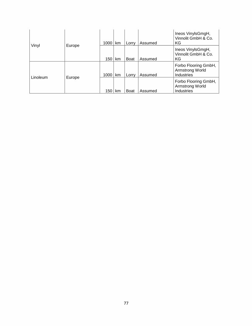
77

Vinyl Europe 1000 km Lorry Assumed

Ineos VinylsGmgH, Vinnolit GmbH & Co. KG

150 km Boat Assumed

Ineos VinylsGmgH, Vinnolit GmbH & Co. KG

Linoleum Europe 1000 km Lorry Assumed

Forbo Flooring GmbH, Armstrong World Industries

150 km Boat Assumed

Forbo Flooring GmbH, Armstrong World Industries

78

Appendix C: Architectural Drawings

Figure 24: Exterior Wall Details

Drawing reference #: 42000A230H554

79

Figure 25: Composition of Interior Walls 1

80

Figure 26: Composition of Interior Walls 2

81

Figure 27: Technical Drawing – Main Building Roof

Drawing reference #: 42000A230H007

82

Figure 28: Technical Drawing – Auditorium Roof

Drawing reference #: 42000A270J013

83

Appendix D: Demolition Report

Method of disposal (Enter quantity and delivery location)

Waste types that are expected to occur in the measure.

Amount delivered to an approved waste facility

Amount for reuse or directly to recycling Delivery Location

Wood is not creosote and CCA-treated 966.06 - Retura TRV

Paper, cardboard and cardboard - - Be delivered as mixed

Glass - - Be delivered as mixed

Iron and other metals - 2881.52 Metallco AS Gypsum-based materials - 199.24 Retura TRV

Plastic - - Be delivered as mixed

Concrete, brick, Leca and other heavy building materials - 40039

Reuse St. Olav's Hospital

Contaminated concrete and brick (below the threshold for hazardous by the fall) 7901 8202

Reuse St. Olav's Hospital! (fine fractions submitted approved reception)

Other hazardous waste - - WEEE 91.9 MetallcoAS Total sorted hazardous waste 8958.96 51321.76 Mixed case of / waste 2160.01 - Retura TRV Total hazardous waste 11118.97 51321.76 Asphalt (not total amount) - - Hazardous waste

type of Waste

Amount delivered to an approved waste facility

Amount for reuse or directly to recycling Delivery Location

7021-23 Oil-containing wastes 0.24 - Retura TRV 7041-42 organic solvents - - 7051-55 Paint, glue, paint, sealants, spray cans etc. (also "empty" syringe cartridges!) 0.27 - Retura TRV 7081 Mercury-containing waste 0.3 - Retura TRV 7086 Fluorescent 1.58 - Retura TRV 7092 Lead accumulators 0.336 - Retura TRV 7098 Pressure treated wood (CCA) 4.48 - Retura TRV

84

7121-23 polymerize substance, isocyanates and hardeners - - 7151 Organic waste containing halogen (eg. Foam) 0.84 - Retura TRV 7152 Organic waste without halogen 71.56 - Retura TRV 7155 Waste with brominated flame retardants (mainly plastics) 1.08 - Retura TRV 7210 PCB and PCT wastes (various) 35.78 - Retura TRV 7210 PCB and PCT waste (sealants) 1.58 - Retura TRV 7211 PCB-containing insulating 10.88 - Retura TRV 7154 Creosote-treated wood 10.08 - Retura TRV 7240 CFC / HCFC / HFC and fluorocarbons (from cooling systems, etc.) - - 7250 Asbestos 136.06 - Retura TRV Other hazardous waste - - Flooring with phthalates 122.26 - Retura TRV Total hazardous waste 397.326 -

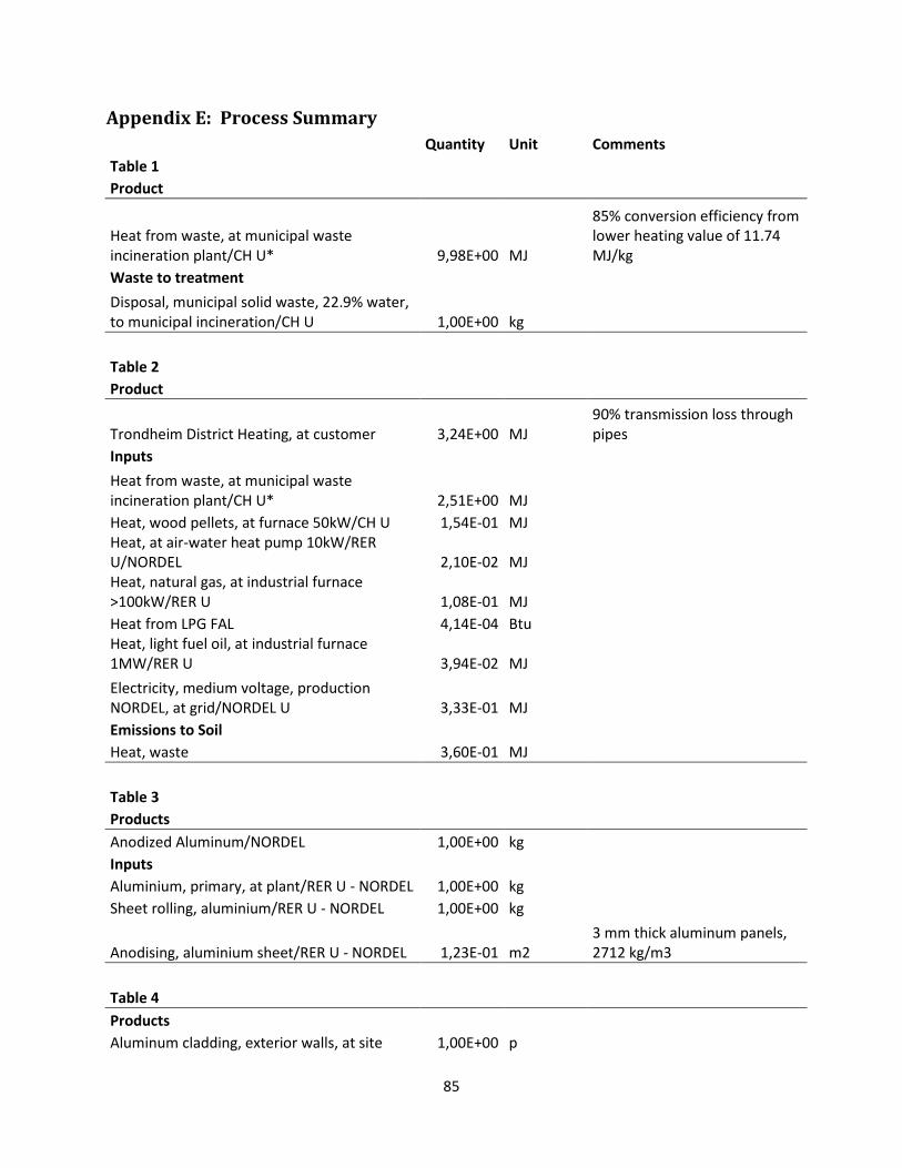
85

Appendix E: Process Summary

Quantity Unit Comments

Table 1 Product

Heat from waste, at municipal waste incineration plant/CH U* 9,98E+00 MJ

85% conversion efficiency from lower heating value of 11.74 MJ/kg

Waste to treatment Disposal, municipal solid waste, 22.9% water,

to municipal incineration/CH U 1,00E+00 kg

Table 2 Product

Trondheim District Heating, at customer 3,24E+00 MJ 90% transmission loss through pipes

Inputs Heat from waste, at municipal waste

incineration plant/CH U* 2,51E+00 MJ Heat, wood pellets, at furnace 50kW/CH U 1,54E-01 MJ Heat, at air-water heat pump 10kW/RER

U/NORDEL 2,10E-02 MJ Heat, natural gas, at industrial furnace

>100kW/RER U 1,08E-01 MJ Heat from LPG FAL 4,14E-04 Btu Heat, light fuel oil, at industrial furnace

1MW/RER U 3,94E-02 MJ Electricity, medium voltage, production

NORDEL, at grid/NORDEL U 3,33E-01 MJ Emissions to Soil

Heat, waste 3,60E-01 MJ

Table 3 Products Anodized Aluminum/NORDEL 1,00E+00 kg

Inputs Aluminium, primary, at plant/RER U - NORDEL 1,00E+00 kg

Sheet rolling, aluminium/RER U - NORDEL 1,00E+00 kg

Anodising, aluminium sheet/RER U - NORDEL 1,23E-01 m2 3 mm thick aluminum panels, 2712 kg/m3

Table 4 Products

Aluminum cladding, exterior walls, at site 1,00E+00 p

86

Inputs Anodized Aluminum/NORDEL 1,13E+04 kg aluminum cladding

Anodized Aluminum/NORDEL 3,19E+03 kg glass fasteners Anodized Aluminum/NORDEL 9,77E+03 kg parapet cladding

Anodized Aluminum/NORDEL 2,23E+04 kg aluminum siding - floor transitions

Transport, lorry 20-28t, fleet average/CH U 3,50E+04 tkm aluminum transport to melting site (750 km)

Table 5 Products Glass cladding, at site 1,00E+00 p

Inputs Flat glass, uncoated, at plant/RER U 3,38E+04 kg 2600 kg/m3

Transport, lorry 20-28t, fleet average/CH U 8,78E+04 tkm 1140 km Transport, transoceanic tanker/OCE U 1,23E+04 tkm 160 km

Table 6 Products

Exterior Walls 1,00E+00 p Inputs

Insulation, exterior walls, at site 1,00E+00 p Reinforced concrete, at site, 5.3%

steel/NORDEL U 9,79E+02 m3 Gypsum plaster board, at site - NORDEL 1,41E+02 m3

Alkyd paint, white, 60% in H2O, at plant/RER U - NORDEL 1,20E+03 kg

0,2216 kg/m2 of gypsum; assuming 0,026 m thick gypsum layering

Transport, lorry 20-28t, fleet average/CH U 1,80E+01 tkm paint transport to site, assuming 15 km transport

Plywood, outdoor use, at site - NORDEL 1,81E+01 m3 timber framing, at site, kiln dried 1,36E+05 kg Vapour Barrier, at site 3,88E+03 m2 Wind barrier, at site 3,88E+03 m2 Fibre cement facing tile, at site - NORDEL 8,44E+00 m3

Table 7 Products Insulation, exterior walls, at site 1,00E+00 p

Inputs Polystyrene foam slab, at site/RER U - 2,51E+02 m3

87

NORDEL

Polystyrene, extruded (XPS) CO2 blown, at site/RER U - NORDEL 2,10E+02 m3

Rockwool, packed, at site - NORDEL 1,80E+03 m3

Table 8 Products Glass curtain wall, at site 1,00E+00 p

Inputs Cladding, crossbar-pole, aluminium, at

plant/RER U/NORDEL 2,70E+03 m2 55.77 kg/m2 Transport, lorry 20-28t, fleet average/CH U 1,50E+04 tkm transport to site (100 km)

Table 9 Products Windows with aluminum frame, at site 1,00E+00 p

Inputs Window frame, aluminium, U=1.6 W/m2K, at

plant/NORDEL 1,54E+02 m2 50.7 kg/m2 Glazing, triple (3-IV), U<0.5 W/m2K, at Lian/NORDEL 8,35E+02 m2 30,12 kg/m2 Glazing, single, at Lian /RER U - NORDEL 1,21E+02 m2 9,005748 kg/m2 Transport, lorry 20-28t, fleet average/CH U 3,40E+03 tkm 100 km to site

Table 10 Products Doors, exterior, aluminum frame, at site 1,00E+00 p

Inputs Window frame, aluminium, U=1.6 W/m2K, at

plant/NORDEL 8,72E+01 m2 50,7 kg/m2 Glazing, triple (3-IV), U<0.5 W/m2K, at Lian/NORDEL 1,17E+02 m2 30 kg/m2 Transport, lorry 20-28t, fleet average/CH U 7,92E+02 tkm 100 km

Table 11 Products Curtain wall, interior 1,00E+00 p

Inputs Glazing, double (2-IV), U<1.1 W/m2K, at

Lian/NORDEL 2,45E+03 m2 sound proof windows Glazing, single, at Lian /RER U - NORDEL 8,66E+02 m2 regular windows

88

Aluminium, primary, at plant/RER U - NORDEL 2,24E+03 kg 2712 kg/m3 Sheet rolling, aluminium/RER U - NORDEL 2,24E+03 kg

Powder coating, aluminium sheet/RER U 3,15E+01 m2

Transport, lorry 20-28t, fleet average/CH U 1,68E+03 tkm alluminum transport (750 km) timber framing, at site, kiln dried 1,90E+03 kg 500 kg/m3 Acrylic binder, 34% in H2O, at plant/RER U 2,34E+00 kg

Acrylic dispersion, 65% in H2O, at plant/RER U 3,52E+01 kg Acrylic varnish, 87.5% in H2O, at plant/RER U 3,52E+01 kg Door, inner, wood, no frame, at site/RER U -

NORDEL 2,95E+02 m2 15,39 kg/m2 Door, inner, glass-wood, no-frame, at site/RER U/NORDEL 5,27E+02 m2 27,6 kg/m2

Table 12 Products Inner doors, steel, at site 1,00E+00 p

Inputs Door, inner, steel, at plant/NORDEL U 2,85E+02 m2 32 kg/m2

Glazing, single, at Lian /RER U - NORDEL 5,48E+01 m2 9 kg/m2 Transport, lorry 20-28t, fleet average/CH U 9,60E+01 tkm transport to site 10 km

Table 13 Products Interior doors, at site 1,00E+00 p

Inputs Door, inner, wood, no frame, at site/RER U -

NORDEL 6,68E+02 m2 Door, inner, glass-wood, no-frame, at

site/RER U/NORDEL 2,28E+02 m2 Inner doors, steel, at site 1,00E+00 p Door frame, inner, steel, at plant/RER U -

NORDEL 1,34E+03 m2 10,5 kg/m2 Transport, lorry 20-28t, fleet average/CH U 6,68E+02 tkm steel transport (500 km) Glazing, single, at Lian /RER U - NORDEL 1,55E+01 m2

Table 14 Products Interior Walls, at site 1,00E+00 p

Inputs Reinforced concrete, at site, 5.3%

steel/NORDEL U 7,39E+02 m3 timber framing, at site, kiln dried 2,40E+03 kg assuming 500 kg/m3

89

Galvinized steel studs, at site - NORDEL 1,02E+01 m3 Gypsum plaster board, at site - NORDEL 6,65E+02 m3 density of 720 kg/m3

Alkyd paint, white, 60% in H2O, at plant/RER U - NORDEL 5,67E+03 kg

plasterboard painting with paint requirement of 0,2216 kg/m2, assuming plaster board thickness of 0,026m

Transport, lorry 20-28t, fleet average/CH U 8,50E+01 tkm paint transport to site (15 km) Rockwool, packed, at site - NORDEL 3,55E+02 m3 assuming 50 kg/m3 Plywood, indoor use, at site - NORDEL 3,81E+00 m3 plywood density (500 kg/m3)

Light mortar, at plant/CH U 4,92E+03 kg light mortar density (405 kg/m3)

Transport, lorry 20-28t, fleet average/CH U 7,38E+01 tkm concrete transport (15 km) Clay plaster, at plant/CH U 1,02E+03 kg plaster density (850 kg/m3) Transport, lorry 20-28t, fleet average/CH U 1,53E+01 tkm plaster transport (15 km) Medium density fibreboard, at site - NORDEL 1,34E+01 m3 density (575 kg/m3) Wind barrier, at site 1,82E+00 m2

Table 15 Products Auditorium Roof, at site 1,00E+00 p

Inputs Glued laminated timber, outdoor use, at

plant/RER U 6,78E+01 m3 glulam density 500 kg/m3

Transport, lorry 20-28t, fleet average/CH U 5,06E+03 tkm glulam transport to site (150 km)

Polystyrene foam slab, at site/RER U - NORDEL 1,18E+02 m3

Polystyrene, extruded (XPS) CO2 blown, at site/RER U - NORDEL 1,18E+02 m3

Zinc, sheet/GLO 3,08E+03 kg zinc density 7135 kg/m3

Transport, lorry 20-28t, fleet average/CH U 1,54E+03 tkm zinc transport to site (500 km)

Transport, transoceanic freight ship/OCE U 6,16E+03 tkm zinc transport to site (2000 km) Plywood, outdoor use, at site - NORDEL 2,78E+01 m3

Cladding, crossbar-pole, aluminium, at plant/RER U/NORDEL 1,12E+02 m2 specific mass (55.77 kg/m2)

Transport, lorry 20-28t, fleet average/CH U 6,25E+02 tkm crossbar transport to site (100km)

Window frame, aluminium, U=1.6 W/m2K, at plant/NORDEL 9,49E+00 m2 specific mass 50,7 kg / m2

90

Transport, lorry 20-28t, fleet average/CH U 4,81E+01 tkm window fram 100 km transport to site

Glazing, triple (3-IV), U<0.5 W/m2K, at Lian/NORDEL 5,38E+01 m2 specific mass 30,12 kg / m2

Transport, lorry 20-28t, fleet average/CH U 1,62E+02 tkm glazing 100 km transport to site Vapour Barrier, at site 6,17E+02 m2

Table 16 Products Ceilings, coverings, at site 1,00E+00 p

Inputs Gypsum plaster board, at site - NORDEL 3,02E+02 m3 720 kg/m3

Plywood, indoor use, at site - NORDEL 1,73E+00 m3 500 kg/m3 Rockwool, packed, at site - NORDEL 1,49E+02 m3 50 kg/m3 Polystyrene, extruded (XPS) CO2 blown, at site/RER U - NORDEL 7,09E+00 m3

Polystyrene foam slab, at site/RER U - NORDEL 7,09E+00 m3

Galvinized steel studs, at site - NORDEL 2,11E+00 m3 Fibre cement facing tile, at site - NORDEL 2,40E+01 m3 1900 kg/m3

Reinforcing steel, at plant/RER U - NORDEL 1,78E+04 kg

Transport, lorry 20-28t, fleet average/CH U 8,91E+03 tkm steel transport to site (500 km) Alkyd paint, white, 60% in H2O, at plant/RER U - NORDEL 2,58E+03 kg

Transport, lorry 20-28t, fleet average/CH U 3,87E+01 tkm

paint transport to site assuming 0,026m thick plaster board layer and 15 km transport to site

Table 17 Products Floors, coverings, at site 1,00E+00 p

Inputs Glued laminated timber, outdoor use, at

plant/NORDEL 1,27E+00 m3 assumed density of 500 kg/m3 Transport, lorry 20-28t, fleet average/CH U 9,53E+01 tkm transport to site150 km

Acrylic varnish, 87.5% in H2O, at plant/RER U 1,57E+01 kg varnish transport to site (15 km)

Transport, lorry 20-28t, fleet average/CH U 2,36E-01 tkm Ceramic tiles, at regional storage/CH U 4,60E+03 kg assume 2500 kg/m3

Transport, lorry 20-28t, fleet average/CH U 2,30E+02 tkm tile transport

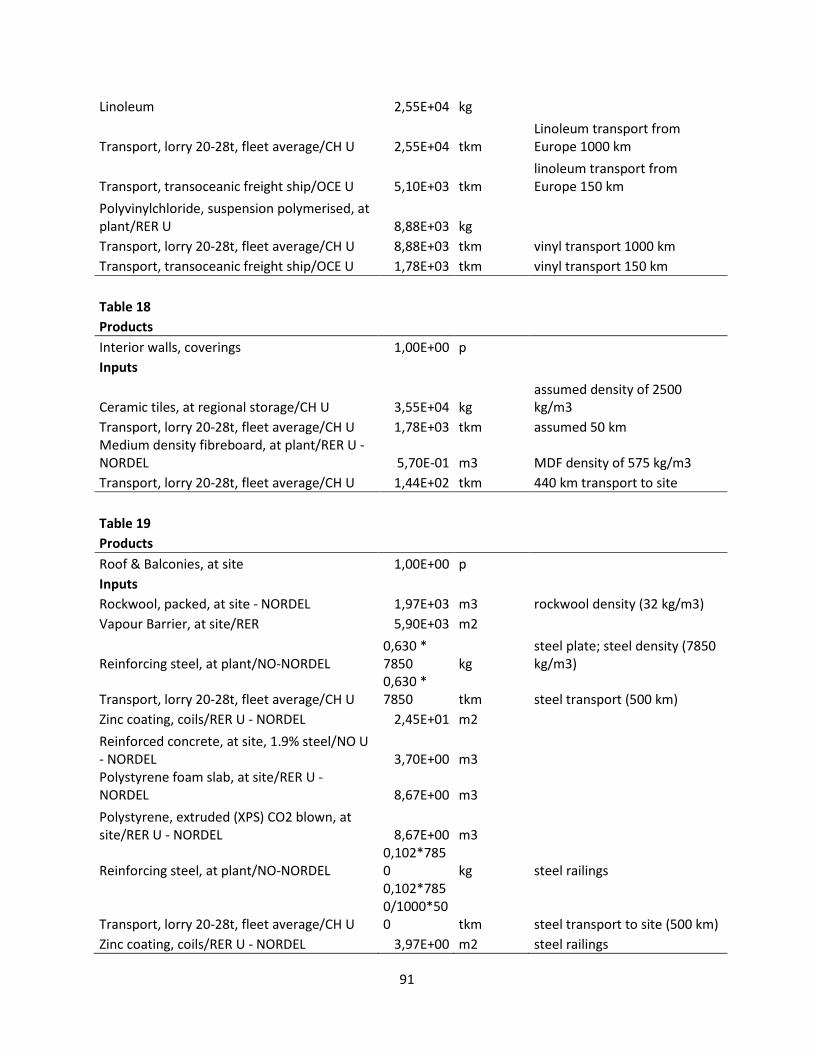
91

Linoleum 2,55E+04 kg

Transport, lorry 20-28t, fleet average/CH U 2,55E+04 tkm Linoleum transport from Europe 1000 km

Transport, transoceanic freight ship/OCE U 5,10E+03 tkm linoleum transport from Europe 150 km

Polyvinylchloride, suspension polymerised, at plant/RER U 8,88E+03 kg

Transport, lorry 20-28t, fleet average/CH U 8,88E+03 tkm vinyl transport 1000 km Transport, transoceanic freight ship/OCE U 1,78E+03 tkm vinyl transport 150 km

Table 18 Products Interior walls, coverings 1,00E+00 p

Inputs

Ceramic tiles, at regional storage/CH U 3,55E+04 kg assumed density of 2500 kg/m3

Transport, lorry 20-28t, fleet average/CH U 1,78E+03 tkm assumed 50 km Medium density fibreboard, at plant/RER U - NORDEL 5,70E-01 m3 MDF density of 575 kg/m3 Transport, lorry 20-28t, fleet average/CH U 1,44E+02 tkm 440 km transport to site

Table 19 Products Roof & Balconies, at site 1,00E+00 p

Inputs Rockwool, packed, at site - NORDEL 1,97E+03 m3 rockwool density (32 kg/m3)

Vapour Barrier, at site/RER 5,90E+03 m2

Reinforcing steel, at plant/NO-NORDEL 0,630 * 7850 kg

steel plate; steel density (7850 kg/m3)

Transport, lorry 20-28t, fleet average/CH U 0,630 * 7850 tkm steel transport (500 km)

Zinc coating, coils/RER U - NORDEL 2,45E+01 m2 Reinforced concrete, at site, 1.9% steel/NO U

- NORDEL 3,70E+00 m3 Polystyrene foam slab, at site/RER U -

NORDEL 8,67E+00 m3 Polystyrene, extruded (XPS) CO2 blown, at

site/RER U - NORDEL 8,67E+00 m3

Reinforcing steel, at plant/NO-NORDEL 0,102*7850 kg steel railings

Transport, lorry 20-28t, fleet average/CH U

0,102*7850/1000*500 tkm steel transport to site (500 km)

Zinc coating, coils/RER U - NORDEL 3,97E+00 m2 steel railings

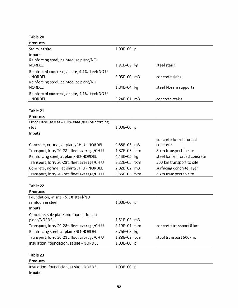
92

Table 20 Products Stairs, at site 1,00E+00 p

Inputs Reinforcing steel, painted, at plant/NO-

NORDEL 1,81E+03 kg steel stairs Reinforced concrete, at site, 4.4% steel/NO U - NORDEL 3,05E+00 m3 concrete slabs Reinforcing steel, painted, at plant/NO-NORDEL 1,84E+04 kg steel I-beam supports Reinforced concrete, at site, 4.4% steel/NO U - NORDEL 5,24E+01 m3 concrete stairs

Table 21 Products Floor slabs, at site - 1.9% steel/NO reinforcing

steel 1,00E+00 p Inputs

Concrete, normal, at plant/CH U - NORDEL 9,85E+03 m3

concrete for reinforced concrete

Transport, lorry 20-28t, fleet average/CH U 1,87E+05 tkm 8 km transport to site Reinforcing steel, at plant/NO-NORDEL 4,43E+05 kg steel for reinforced concrete Transport, lorry 20-28t, fleet average/CH U 2,22E+05 tkm 500 km transport to site Concrete, normal, at plant/CH U - NORDEL 2,02E+02 m3 surfacing concrete layer Transport, lorry 20-28t, fleet average/CH U 3,85E+03 tkm 8 km transport to site

Table 22 Products Foundation, at site - 5.3% steel/NO

reinfocring steel 1,00E+00 p Inputs

Concrete, sole plate and foundation, at plant/NORDEL 1,51E+03 m3

Transport, lorry 20-28t, fleet average/CH U 3,19E+01 tkm concrete transport 8 km Reinforcing steel, at plant/NO-NORDEL 3,76E+03 kg

Transport, lorry 20-28t, fleet average/CH U 1,88E+03 tkm steel transport 500km, Insulation, foundation, at site - NORDEL 1,00E+00 p

Table 23 Products Insulation, foundation, at site - NORDEL 1,00E+00 p

Inputs

93

Polystyrene foam slab, at site/RER U - NORDEL 7,42E+01 m3

Polystyrene, extruded (XPS) CO2 blown, at site/RER U - NORDEL 7,42E+01 m3

Table 24 Products Load bearing walls, at site - 5.0% steel/NO

reinforcing steel 1,00E+00 p Inputs

Concrete, normal, at plant/CH U - NORDEL 1,37E+03 m3

Transport, lorry 20-28t, fleet average/CH U 2,60E+04 tkm concrete transport to site (8km)

Reinforcing steel, at plant/NO-NORDEL 1,71E+05 kg 123 kg steel /m3 wall Transport, lorry 20-28t, fleet average/CH U 8,55E+04 tkm

Table 25 Products Insulation, load bearing walls, at site -

NORDEL 1,00E+00 p Inputs

Polystyrene foam slab, at site/RER U - NORDEL 2,63E+01 m3

Polystyrene, extruded (XPS) CO2 blown, at site/RER U - NORDEL 2,63E+01 m3

Table 26 Products Reinforced concrete beams, at site - 7.0%

steel/NO reinforcing steel 1,00E+00 p Inputs

Concrete, normal, at plant/CH U - NORDEL 4,21E+01 m3

concrete transport to site (8km)

Transport, lorry 20-28t, fleet average/CH U 8,02E+02 tkm steel density 7850 kg/m3 Reinforcing steel, at plant/NO-NORDEL 8,68E+03 kg steel transport 500 km to site Transport, lorry 20-28t, fleet average/CH U 4,34E+03 tkm

Table 27 Products Reinforced concrete columns, at site - 4.5%

steel/NO reinforcing steel 1,00E+00 p Inputs

Concrete, normal, at plant/CH U - NORDEL 4,39E+02 m3

94

Transport, lorry 20-28t, fleet average/CH U 8,36E+03 tkm concrete transport 8km to site Reinforcing steel, at plant/NO-NORDEL 5,41E+04 kg steel density 7850 kg/m3 Transport, lorry 20-28t, fleet average/CH U 2,70E+04 tkm steel transport to site

Table 28 Products Steel columns, at site/NO reinforcing steel 1,00E+00 p 100

Inputs Reinforcing steel, painted, at plant/NO-

NORDEL 2,06E+05 kg 7850 kg/m3 + additional paint mass of 0.2%

Transport, lorry 20-28t, fleet average/CH U 1,03E+05 tkm steel transport to site (500 km)

Table 29 Products Steel beams, at site/NO reinforcing steel 1,00E+00 p

Inputs Reinforcing steel, painted, at plant/NO-

NORDEL 5,04E+04 kg 7850 kg/m3 Transport, lorry 20-28t, fleet average/CH U 2,52E+04 tkm 500 km

Table 30 Products

Glazing, single, at Lian /RER U - NORDEL 1,00E+00 m2

Reference Process: Glazing, double (2-IV), U<1.1 W/m2K, at plant/RER U

Inputs Water, completely softened, at plant/RER U 4,98E-01 kg

Flat glass, uncoated, at plant/RER U 9,68E+00 kg Electricity, low voltage, production NORDEL,

at grid/NORDEL U 1,60E+00 kWh Transport, lorry 20-28t, fleet average/CH U 1,55E+01 tkm 1600 km

Transport, transoceanic freight ship/OCE U 9,68E-01 tkm 100 km Emissions to air

Heat, waste

11,554/2 MJ Waste to treatment

Disposal, glass, 0% water, to inert material landfill/CH U

1,35570000000000013/2 kg

Treatment, sewage, unpolluted, to wastewater treatment, class 3/CH U 4,98E-04 m3

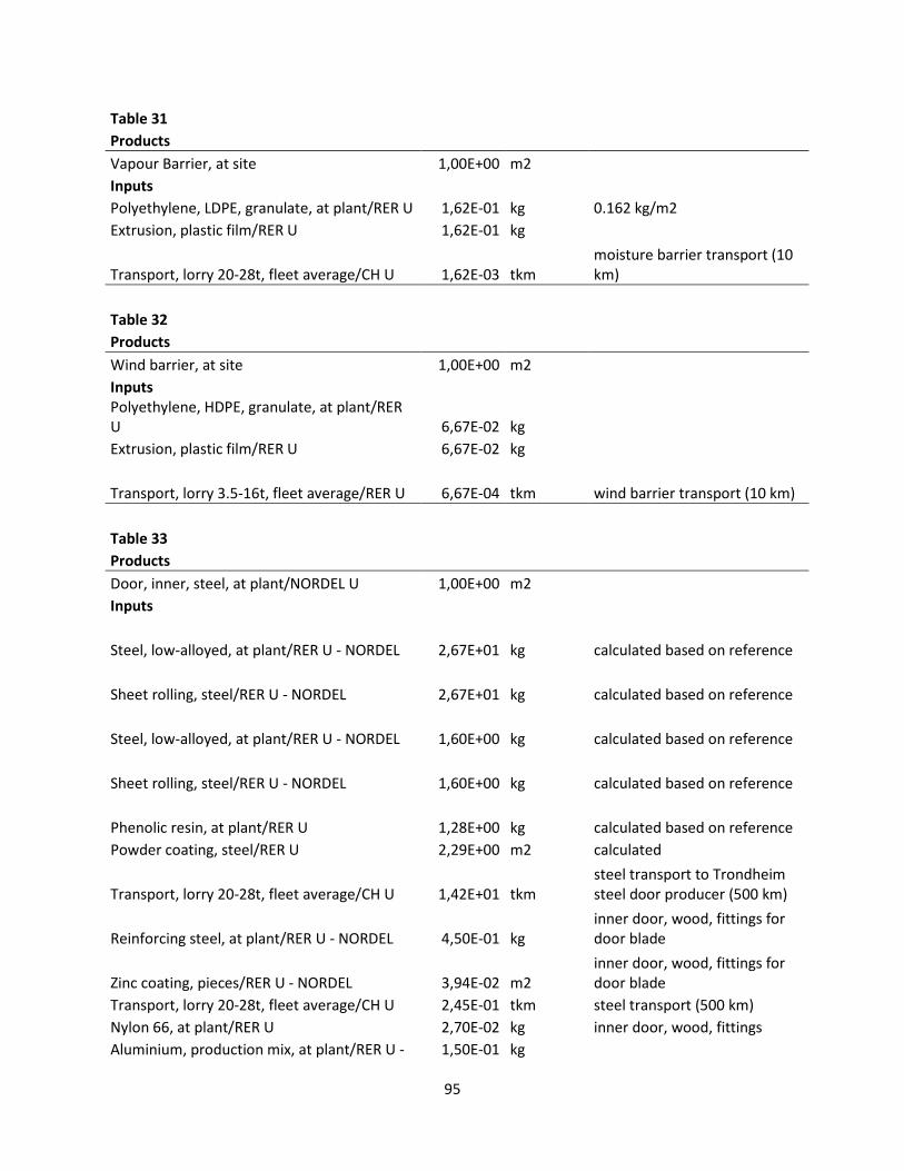
95

Table 31 Products Vapour Barrier, at site 1,00E+00 m2

Inputs Polyethylene, LDPE, granulate, at plant/RER U 1,62E-01 kg 0.162 kg/m2

Extrusion, plastic film/RER U 1,62E-01 kg

Transport, lorry 20-28t, fleet average/CH U 1,62E-03 tkm moisture barrier transport (10 km)

Table 32 Products Wind barrier, at site 1,00E+00 m2

Inputs Polyethylene, HDPE, granulate, at plant/RER

U 6,67E-02 kg Extrusion, plastic film/RER U 6,67E-02 kg

Transport, lorry 3.5-16t, fleet average/RER U 6,67E-04 tkm wind barrier transport (10 km)

Table 33 Products Door, inner, steel, at plant/NORDEL U 1,00E+00 m2

Inputs

Steel, low-alloyed, at plant/RER U - NORDEL 2,67E+01 kg calculated based on reference

Sheet rolling, steel/RER U - NORDEL 2,67E+01 kg calculated based on reference

Steel, low-alloyed, at plant/RER U - NORDEL 1,60E+00 kg calculated based on reference

Sheet rolling, steel/RER U - NORDEL 1,60E+00 kg calculated based on reference

Phenolic resin, at plant/RER U 1,28E+00 kg calculated based on reference Powder coating, steel/RER U 2,29E+00 m2 calculated

Transport, lorry 20-28t, fleet average/CH U 1,42E+01 tkm steel transport to Trondheim steel door producer (500 km)

Reinforcing steel, at plant/RER U - NORDEL 4,50E-01 kg inner door, wood, fittings for door blade

Zinc coating, pieces/RER U - NORDEL 3,94E-02 m2 inner door, wood, fittings for door blade

Transport, lorry 20-28t, fleet average/CH U 2,45E-01 tkm steel transport (500 km) Nylon 66, at plant/RER U 2,70E-02 kg inner door, wood, fittings Aluminium, production mix, at plant/RER U - 1,50E-01 kg

96

NORDEL Transport, lorry 20-28t, fleet average/CH U 1,13E-01 tkm aluminum transport (750 km) Anodising, aluminium sheet/RER U - NORDEL 1,38E-02 m2

Lubricating oil, at plant/RER U 1,34E-02 kg inner door, wood, fittings Polyethylene, LLDPE, granulate, at plant/RER U 6,25E-01 kg

Diesel, burned in building machine/GLO U 2,47E+00 MJ inner door, wood, door blade Natural gas, burned in industrial furnace >100kW/RER U 3,96E-02 MJ inner door, wood, fittings Electricity, medium voltage, production NORDEL, at grid/NORDEL U 4,08E+00 kWh inner door, wood, door blade

Metal working factory/RER/I U 1,26E-08 p inner door, wood, infrastructure

Emissions to air Heat, waste 14,7 MJ

Waste to treatment Disposal, inert material, 0% water, to sanitary

landfill/CH U 6,06E-03 kg Disposal, municipal solid waste, 22.9% water,

to municipal incineration/CH U 2,44E-02 kg Disposal, polyethylene, 0.4% water, to

municipal incineration/CH U 6,25E-01 kg

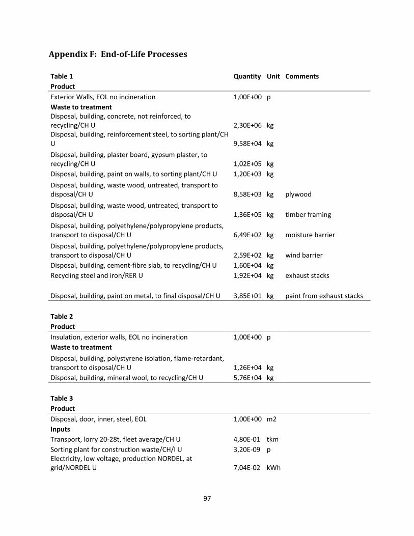
97

Appendix F: End-of-Life Processes

Table 1 Quantity Unit Comments Product

Exterior Walls, EOL no incineration 1,00E+00 p Waste to treatment

Disposal, building, concrete, not reinforced, to recycling/CH U 2,30E+06 kg

Disposal, building, reinforcement steel, to sorting plant/CH U 9,58E+04 kg

Disposal, building, plaster board, gypsum plaster, to recycling/CH U 1,02E+05 kg

Disposal, building, paint on walls, to sorting plant/CH U 1,20E+03 kg Disposal, building, waste wood, untreated, transport to

disposal/CH U 8,58E+03 kg plywood Disposal, building, waste wood, untreated, transport to disposal/CH U 1,36E+05 kg timber framing Disposal, building, polyethylene/polypropylene products, transport to disposal/CH U 6,49E+02 kg moisture barrier Disposal, building, polyethylene/polypropylene products, transport to disposal/CH U 2,59E+02 kg wind barrier Disposal, building, cement-fibre slab, to recycling/CH U 1,60E+04 kg

Recycling steel and iron/RER U 1,92E+04 kg exhaust stacks

Disposal, building, paint on metal, to final disposal/CH U 3,85E+01 kg paint from exhaust stacks

Table 2 Product Insulation, exterior walls, EOL no incineration 1,00E+00 p

Waste to treatment Disposal, building, polystyrene isolation, flame-retardant,

transport to disposal/CH U 1,26E+04 kg Disposal, building, mineral wool, to recycling/CH U 5,76E+04 kg

Table 3 Product Disposal, door, inner, steel, EOL 1,00E+00 m2

Inputs Transport, lorry 20-28t, fleet average/CH U 4,80E-01 tkm

Sorting plant for construction waste/CH/I U 3,20E-09 p Electricity, low voltage, production NORDEL, at

grid/NORDEL U 7,04E-02 kWh

98

Excavation, hydraulic digger/RER U 5,00E-02 m3 sorting plant electricity use

Waste to treatment

machinery at sorting plant Recycling aluminium/RER U 1,50E-01 kg

Recycling steel and iron/RER U 2,88E+01 kg Disposal, inert waste, 5% water, to inert material

landfill/CH U 3,94E-02 kg

Table 4 Product Disposal, doors, aluminum frame, at site - NORDEL 1,00E+00 p

Waste to treatment Disposal, window frame, aluminium, U=1.6

W/m2K/NORDEL 8,72E+01 m2 Disposal, glazing, triple (3-IV), U<0.5 W/m2K/NORDEL 1,17E+02 m2

Table 5 Product Disposal, glazing, double (2-IV), U<1.1 W/m2K/NORDEL 1,00E+00 m2

Inputs

Transport, lorry 20-28t, fleet average/CH U 3,01E-01 tkm transport to sorting plant (15 km)

Excavation, skid-steer loader/RER U 2,08E-02 m3

double glazed window density 866.7 kg /m3; bulk density adjustment factor 0,9

Sorting plant for construction waste/CH/I U 2,01E-09 p Electricity, low voltage, production NORDEL, at

grid/NORDEL U 7,42E-02 kWh Waste to treatment

Disposal, glass, 0% water, to municipal incineration/CH U 1,80E+00 kg Recycling glass/RER U 1,62E+01 kg Disposal, rubber, unspecified, 0% water, to municipal

incineration/CH U 9,37E-03 kg Disposal, zeolite, 5% water, to inert material landfill/CH U 1,32E+00 kg Recycling aluminium/RER U 3,03E-01 kg Disposal, plastics, mixture, 15.3% water, to municipal

incineration/CH U 4,38E-01 kg

Table 6 Product Disposal, glazing, single /RER U/NORDEL 1,00E+00 m2

99

Waste to treatment Recycling glass/RER U 8,56E+00 kg

Disposal, glass, 0% water, to inert material landfill/CH U 4,50E-01 kg

Table 7 Product Disposal, glazing, triple (3-IV), U<0.5 W/m2K/NORDEL 1,00E+00 m2

Inputs

Transport, lorry 20-28t, fleet average/CH U 4,55E-01 tkm transport to sorting plant (15 km)

Excavation, skid-steer loader/RER U 4,75E-02 m3

double glazed window density 709 kg /m3; bulk density adjustment factor 0,9

Sorting plant for construction waste/CH/I U 3,03E-09 p Electricity, low voltage, production NORDEL, at

grid/NORDEL U 1,12E-01 kWh 3,7 kWh per tonne Waste to treatment

Disposal, glass, 0% water, to municipal incineration/CH U 8,72E-01 kg Recycling glass/RER U 2,41E+01 kg Disposal, plastics, mixture, 15.3% water, to municipal

incineration/CH U 6,57E-01 kg Disposal, zeolite, 5% water, to inert material landfill/CH U 1,93E+00 kg Recycling aluminium/RER U 5,20E-01 kg Disposal, rubber, unspecified, 0% water, to municipal

incineration/CH U 1,87E-02 kg

Table 8 Product Disposal, window frame, aluminium, U=1.6

W/m2K/NORDEL 1,00E+00 m2 Inputs

Transport, lorry 20-28t, fleet average/CH U 7,60E-01 tkm

aluminum transport to sorting plant (15 km)

Excavation, skid-steer loader/RER U 1,11E-01 m3 assume 0,1m thick Sorting plant for construction waste/CH/I U 5,07E-09 p

Electricity, low voltage, production NORDEL, at grid/NORDEL U 1,87E-01 kWh

Waste to treatment Disposal, plastics, mixture, 15.3% water, to municipal

incineration/CH U 5,28E+00 kg Disposal, rubber, unspecified, 0% water, to municipal

incineration/CH U 5,27E+00 kg

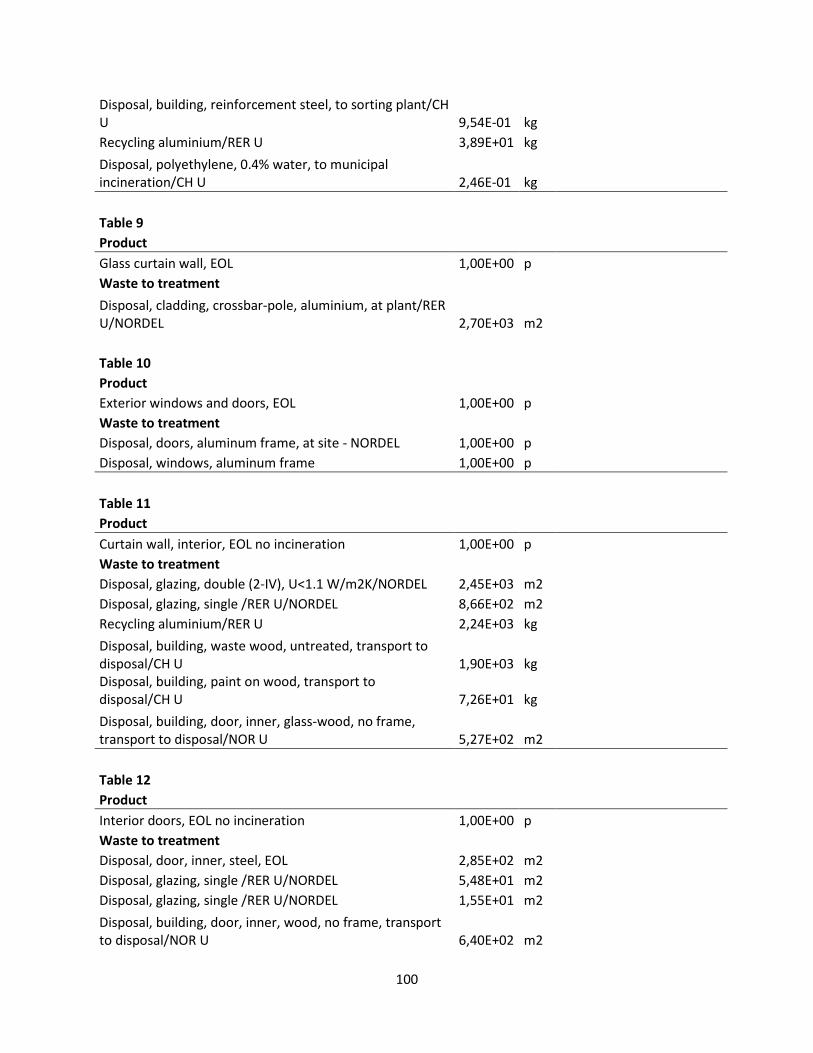
100

Disposal, building, reinforcement steel, to sorting plant/CH U 9,54E-01 kg

Recycling aluminium/RER U 3,89E+01 kg Disposal, polyethylene, 0.4% water, to municipal

incineration/CH U 2,46E-01 kg

Table 9 Product Glass curtain wall, EOL 1,00E+00 p

Waste to treatment Disposal, cladding, crossbar-pole, aluminium, at plant/RER

U/NORDEL 2,70E+03 m2

Table 10 Product Exterior windows and doors, EOL 1,00E+00 p

Waste to treatment Disposal, doors, aluminum frame, at site - NORDEL 1,00E+00 p

Disposal, windows, aluminum frame 1,00E+00 p

Table 11 Product Curtain wall, interior, EOL no incineration 1,00E+00 p

Waste to treatment Disposal, glazing, double (2-IV), U<1.1 W/m2K/NORDEL 2,45E+03 m2

Disposal, glazing, single /RER U/NORDEL 8,66E+02 m2 Recycling aluminium/RER U 2,24E+03 kg Disposal, building, waste wood, untreated, transport to

disposal/CH U 1,90E+03 kg Disposal, building, paint on wood, transport to

disposal/CH U 7,26E+01 kg Disposal, building, door, inner, glass-wood, no frame,

transport to disposal/NOR U 5,27E+02 m2

Table 12 Product Interior doors, EOL no incineration 1,00E+00 p

Waste to treatment Disposal, door, inner, steel, EOL 2,85E+02 m2

Disposal, glazing, single /RER U/NORDEL 5,48E+01 m2 Disposal, glazing, single /RER U/NORDEL 1,55E+01 m2 Disposal, building, door, inner, wood, no frame, transport

to disposal/NOR U 6,40E+02 m2

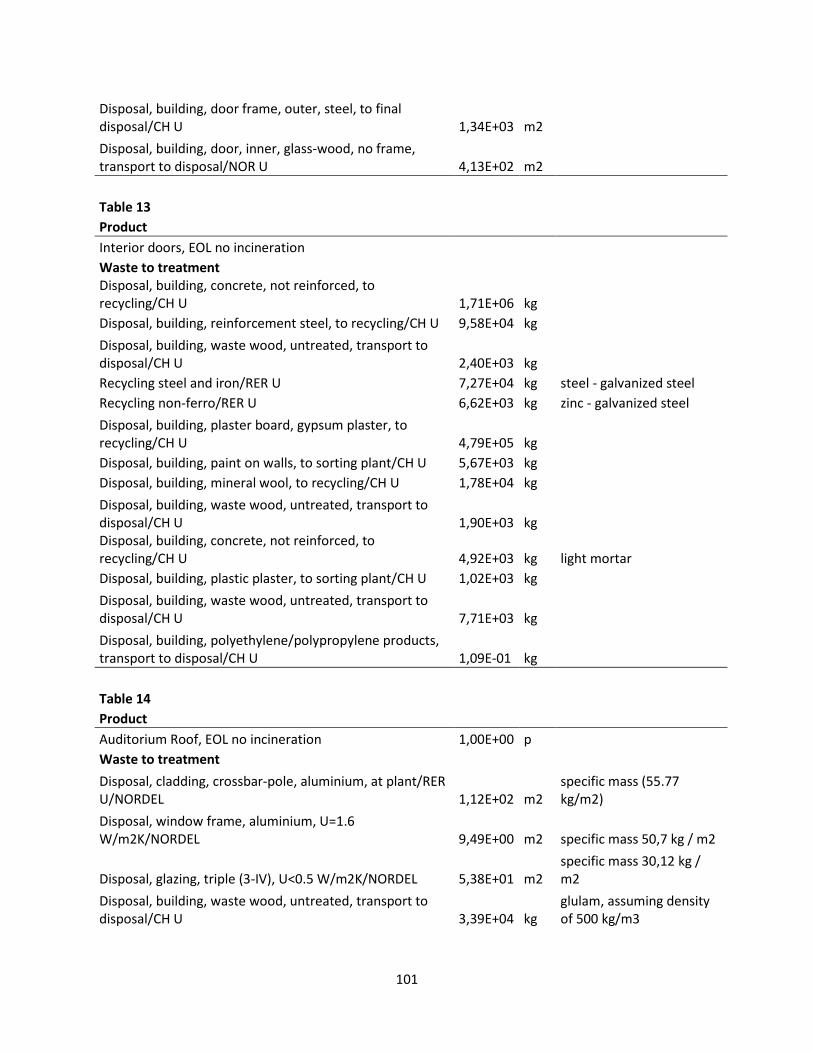
101

Disposal, building, door frame, outer, steel, to final disposal/CH U 1,34E+03 m2

Disposal, building, door, inner, glass-wood, no frame, transport to disposal/NOR U 4,13E+02 m2

Table 13 Product Interior doors, EOL no incineration

Waste to treatment Disposal, building, concrete, not reinforced, to

recycling/CH U 1,71E+06 kg Disposal, building, reinforcement steel, to recycling/CH U 9,58E+04 kg Disposal, building, waste wood, untreated, transport to

disposal/CH U 2,40E+03 kg Recycling steel and iron/RER U 7,27E+04 kg steel - galvanized steel

Recycling non-ferro/RER U 6,62E+03 kg zinc - galvanized steel Disposal, building, plaster board, gypsum plaster, to recycling/CH U 4,79E+05 kg

Disposal, building, paint on walls, to sorting plant/CH U 5,67E+03 kg Disposal, building, mineral wool, to recycling/CH U 1,78E+04 kg Disposal, building, waste wood, untreated, transport to

disposal/CH U 1,90E+03 kg Disposal, building, concrete, not reinforced, to

recycling/CH U 4,92E+03 kg light mortar Disposal, building, plastic plaster, to sorting plant/CH U 1,02E+03 kg

Disposal, building, waste wood, untreated, transport to disposal/CH U 7,71E+03 kg

Disposal, building, polyethylene/polypropylene products, transport to disposal/CH U 1,09E-01 kg

Table 14 Product Auditorium Roof, EOL no incineration 1,00E+00 p

Waste to treatment Disposal, cladding, crossbar-pole, aluminium, at plant/RER

U/NORDEL 1,12E+02 m2 specific mass (55.77 kg/m2)

Disposal, window frame, aluminium, U=1.6 W/m2K/NORDEL 9,49E+00 m2 specific mass 50,7 kg / m2

Disposal, glazing, triple (3-IV), U<0.5 W/m2K/NORDEL 5,38E+01 m2 specific mass 30,12 kg / m2

Disposal, building, waste wood, untreated, transport to disposal/CH U 3,39E+04 kg

glulam, assuming density of 500 kg/m3

102

Disposal, building, polystyrene isolation, flame-retardant, transport to disposal/CH U 3,55E+03 kg

Disposal, building, polystyrene isolation, flame-retardant, transport to disposal/CH U 2,96E+03 kg

Recycling non-ferro/RER U 3,08E+03 kg Disposal, building, waste wood, untreated, transport to

disposal/CH U 1,32E+04 kg plywood, assuming density of 475 kg/m3

Disposal, building, polyethylene/polypropylene products, transport to disposal/CH U 9,93E+01 kg

vapour barrier disposal, specific mass of 0,161 kg/m2

Table 15 Product Stairs, EOL 1,00E+00 p

Waste to treatment Disposal, building, concrete, not reinforced, to

recycling/CH U 1,34E+05 kg Disposal, building, reinforcement steel, to recycling/CH U 2,05E+03 kg Recycling steel and iron/RER U 2,03E+04 kg

Table 16 Product Interior walls, coverings, EOL no incineration 1,00E+00 p

Inputs

Transport, lorry 20-28t, fleet average/CH U 1,78E+03 tkm tile transport to landfill (50 km)

Waste to treatment Disposal, building, waste wood, untreated, transport to

disposal/CH U 3,28E+02 kg Disposal, inert waste, 5% water, to inert material

landfill/CH U 3,55E+04 kg

Table 17 Product Floors, coverings, EOL no incineration 1,00E+00 p

Inputs

Transport, lorry 20-28t, fleet average/CH U 3,82E+02 tkm lineolum transport to incineration

Waste to treatment Disposal, building, waste wood, untreated, to final

disposal/CH U 6,35E+02 kg Disposal, inert waste, 5% water, to inert material

landfill/CH U 4,60E+03 kg

103

Disposal, building, polyvinylchloride products, transport to disposal/CH U 8,88E+03 kg

Waste incineration of biodegradable waste fraction in municipal solid waste (MSW), EU-27 S 2,55E+04 kg

Disposal, building, paint on wood, to final disposal/CH U 1,57E+01 kg

Table 18 Product Ceilings, coverings, EOL no incineration 1,00E+00 p

Waste to treatment Disposal, building, plaster board, gypsum plaster, to

recycling/CH U 2,19E+05 kg Disposal, building, waste wood, untreated, transport to

disposal/CH U 1,77E+03 kg Disposal, building, mineral wool, to recycling/CH U 8,15E+03 kg Recycling steel and iron/RER U 1,51E+04 kg galvinzed steel

Recycling non-ferro/RER U 1,37E+03 kg galvinized steel Disposal, building, cement-fibre slab, to recycling/CH U 4,56E+04 kg

Recycling steel and iron/RER U 2,40E+04 kg ceilings

Table 19 Product Foundation, 5.3% steel, EOL 1,00E+00 p

Waste to treatment Disposal, building, concrete, not reinforced, to

recycling/CH U 3,61E+06 kg Disposal, building, reinforcement steel, to recycling/CH U 2,02E+05 kg

Table 20 Product Insulation, foundation/NORDEL U, EOL no incineration 1,00E+00 p

Waste to treatment Disposal, building, polystyrene isolation, flame-retardant,

transport to disposal/CH U 2,23E+03 kg Disposal, building, polystyrene isolation, flame-retardant,

transport to disposal/CH U 1,86E+03 kg

Table 21 Product Floor slabs, 1.9% steel, EOL 1,00E+00 p

Waste to treatment Disposal, building, concrete, not reinforced, to

recycling/CH U 2,40E+07 kg

104

Disposal, building, reinforcement steel, to recycling/CH U 4,65E+05 kg

Table 22 Product Load bearing walls, 5.0% steel, EOL 1,00E+00 p

Waste to treatment Waste to treatment Disposal, building, concrete, not reinforced, to

recycling/CH U 3,25E+06 kg Disposal, building, reinforcement steel, to recycling/CH U 1,71E+05 kg

Table 23 Product Disposal, insulation, load bearing walls, no incineration 1,00E+00 p

Waste to treatment Disposal, building, polystyrene isolation, flame-retardant,

transport to disposal/CH U 7,89E+02 kg Disposal, building, polystyrene isolation, flame-retardant,

transport to disposal/CH U 6,58E+02 kg

Table 24 Product disposal, reinforced concrete beams, 7.0% steel 1,00E+00 p

Waste to treatment Disposal, building, concrete, not reinforced, to

recycling/CH U 1,00E+05 kg Disposal, building, reinforcement steel, to recycling/CH U 7,54E+03 kg

Table 25 Product disposal, reinforced concrete columns, 4.5% steel 1,00E+00 p

Waste to treatment Disposal, building, concrete, not reinforced, to

recycling/CH U 1,04E+06 kg Disposal, building, reinforcement steel, to recycling/CH U 5,41E+04 kg

Table 26 Product disposal steel beams 1,00E+00 p

Waste to treatment Recycling steel and iron/RER S 5,03E+04 kg

Disposal, building, paint on metal, to final disposal/CH U 1,01E+02 kg

105

Table 27 Product disposal, steel columns 1,00E+00 p

Waste to treatment Recycling steel and iron/RER S 2,05E+05 kg

Disposal, building, paint on metal, to final disposal/CH U 4,11E+02 kg

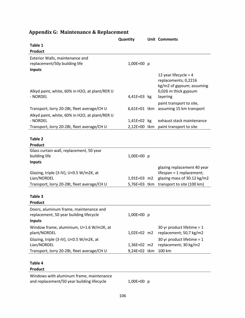
106

Appendix G: Maintenance & Replacement

Quantity Unit Comments

Table 1 Product Exterior Walls, maintenance and

replacement/50y building life 1,00E+00 p Inputs

Alkyd paint, white, 60% in H2O, at plant/RER U - NORDEL 4,41E+03 kg

12 year lifecycle = 4 replacements; 0,2216 kg/m2 of gypsum; assuming 0,026 m thick gypsum layering

Transport, lorry 20-28t, fleet average/CH U 6,61E+01 tkm paint transport to site, assuming 15 km transport

Alkyd paint, white, 60% in H2O, at plant/RER U - NORDEL 1,41E+02 kg exhaust stack maintenance Transport, lorry 20-28t, fleet average/CH U 2,12E+00 tkm paint transport to site

Table 2 Product Glass curtain wall, replacement, 50 year

building life 1,00E+00 p Inputs

Glazing, triple (3-IV), U<0.5 W/m2K, at Lian/NORDEL 1,91E+03 m2

glazing replacement 40 year lifespan = 1 replacement; glazing mass of 30.12 kg/m2

Transport, lorry 20-28t, fleet average/CH U 5,76E+03 tkm transport to site (100 km)

Table 3 Product Doors, aluminum frame, maintenance and

replacement, 50 year building lifecycle 1,00E+00 p Inputs

Window frame, aluminium, U=1.6 W/m2K, at plant/NORDEL 1,02E+02 m2

30 yr product lifetime = 1 replacement; 50,7 kg/m2

Glazing, triple (3-IV), U<0.5 W/m2K, at Lian/NORDEL 1,36E+02 m2

30 yr product lifetime = 1 replacement; 30 kg/m2

Transport, lorry 20-28t, fleet average/CH U 9,24E+02 tkm 100 km

Table 4 Product Windows with aluminum frame, maintenance

and replacement/50 year building lifecycle 1,00E+00 p

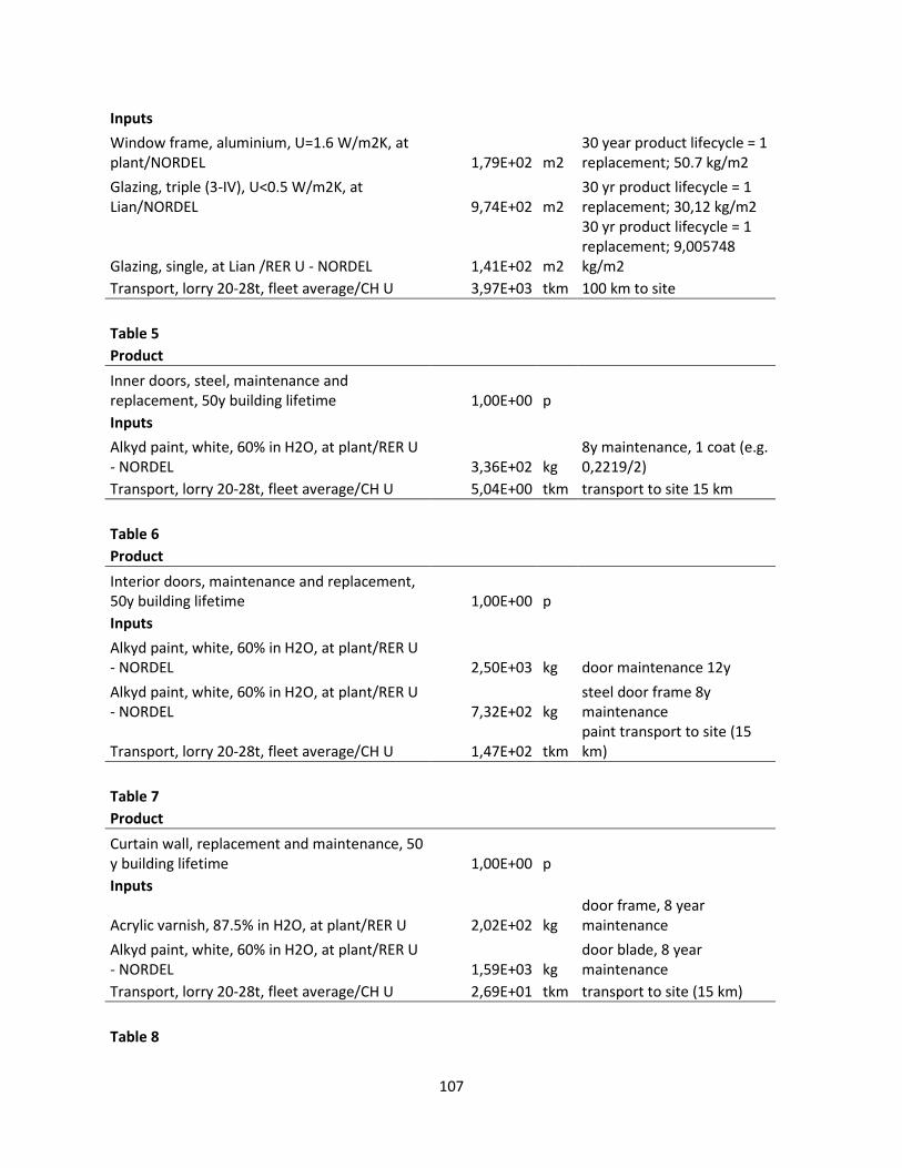
107

Inputs Window frame, aluminium, U=1.6 W/m2K, at

plant/NORDEL 1,79E+02 m2 30 year product lifecycle = 1 replacement; 50.7 kg/m2

Glazing, triple (3-IV), U<0.5 W/m2K, at Lian/NORDEL 9,74E+02 m2

30 yr product lifecycle = 1 replacement; 30,12 kg/m2

Glazing, single, at Lian /RER U - NORDEL 1,41E+02 m2

30 yr product lifecycle = 1 replacement; 9,005748 kg/m2

Transport, lorry 20-28t, fleet average/CH U 3,97E+03 tkm 100 km to site

Table 5 Product Inner doors, steel, maintenance and

replacement, 50y building lifetime 1,00E+00 p Inputs

Alkyd paint, white, 60% in H2O, at plant/RER U - NORDEL 3,36E+02 kg

8y maintenance, 1 coat (e.g. 0,2219/2)

Transport, lorry 20-28t, fleet average/CH U 5,04E+00 tkm transport to site 15 km

Table 6 Product Interior doors, maintenance and replacement,

50y building lifetime 1,00E+00 p Inputs

Alkyd paint, white, 60% in H2O, at plant/RER U - NORDEL 2,50E+03 kg door maintenance 12y Alkyd paint, white, 60% in H2O, at plant/RER U - NORDEL 7,32E+02 kg

steel door frame 8y maintenance

Transport, lorry 20-28t, fleet average/CH U 1,47E+02 tkm paint transport to site (15 km)

Table 7 Product Curtain wall, replacement and maintenance, 50

y building lifetime 1,00E+00 p Inputs

Acrylic varnish, 87.5% in H2O, at plant/RER U 2,02E+02 kg

door frame, 8 year maintenance

Alkyd paint, white, 60% in H2O, at plant/RER U - NORDEL 1,59E+03 kg

door blade, 8 year maintenance

Transport, lorry 20-28t, fleet average/CH U 2,69E+01 tkm transport to site (15 km)

Table 8

108

Product Interior Walls, maintenance and replacement,

50y buiding lifetime 1,00E+00 p Inputs

Alkyd paint, white, 60% in H2O, at plant/RER U - NORDEL

(50/12 - 0,5) * 665,078/0,026 * 0,2216 kg

plaster board painting 12y; plasterboard painting with paint requirement of 0,2216 kg/m2, assuming plaster board thickness of 0,026m

Transport, van <3.5t/CH U 20800/1000 * 15 tkm

paint transport to site (15 km)

Table 9 Product Auditorium Roof, maintenance and

replacement, 50y building lifetime 1,00E+00 p Inputs

Glazing, triple (3-IV), U<0.5 W/m2K, at Lian/NORDEL 5,67E+01 m2 40 year glazing replacement

Transport, lorry 20-28t, fleet average/CH U 5,67E+00 tkm glazing transport to site (100km)

Window frame, aluminium, U=1.6 W/m2K, at plant/NORDEL 7,11E+00 m2

40 year window replacement; specific mass 50,7 kg / m2

Transport, lorry 20-28t, fleet average/CH U 3,61E+01 tkm window fram 100 km transport to site

Glazing, triple (3-IV), U<0.5 W/m2K, at Lian/NORDEL 4,03E+01 m2 specific mass 30,12 kg / m2

Transport, lorry 20-28t, fleet average/CH U 1,21E+02 tkm glazing 100 km transport to site

Table 10 Product Roof & Balconies, maintenance and

replacement/50y building lifetime 1,00E+00 p Inputs

Vapour Barrier, at site/RER 4,43E+03 m2 40y replacement time

Table 11 Product Interior wall coverings, maintenance and

replacement/50y building lifetime 1,00E+00 p Inputs

Ceramic tiles, at regional storage/CH U 7,11E+04 kg

ceramic tiles 30y product replacement; assumed

109

density of 2500 kg/m3

Transport, lorry 20-28t, fleet average/CH U 3,55E+03 tkm Tile transport to site; assumed 50 km

Table 12 Product Floors, coverings, maintenance and

replacement/50y building lifetime 1,00E+00 p Inputs

Acrylic varnish, 87.5% in H2O, at plant/RER U 1,49E+02 kg

varnish transport to site (15 km)

Transport, lorry 20-28t, fleet average/CH U 2,24E+00 tkm Ceramic tiles, at regional storage/CH U 9,20E+03 kg assume 2500 kg/m3

Transport, lorry 20-28t, fleet average/CH U 4,60E+02 tkm tile transport Linoleum 5,10E+04 kg

Transport, lorry 20-28t, fleet average/CH U 5,10E+04 tkm

Linoleum transport from Europe 1000 km

Transport, transoceanic freight ship/OCE U 1,02E+04 tkm linoleum transport from Europe 150 km

Polyvinylchloride, suspension polymerised, at plant/RER U 1,78E+04 kg

Transport, lorry 20-28t, fleet average/CH U 1,78E+04 tkm vinyl transport 1000 km Transport, transoceanic freight ship/OCE U 3,55E+03 tkm vinyl transport 150 km

Table 12 Product Ceilings, coverings, maintenance and

replacement/50y building lifetime 1,00E+00 p Inputs

Alkyd paint, white, 60% in H2O, at plant/RER U - NORDEL 9,45E+03 kg

paint maintenance 12y intervals

Transport, lorry 20-28t, fleet average/CH U 1,42E+02 tkm

paint transport to site assuming 0,026m thick plaster board layer and 15 km transport to site

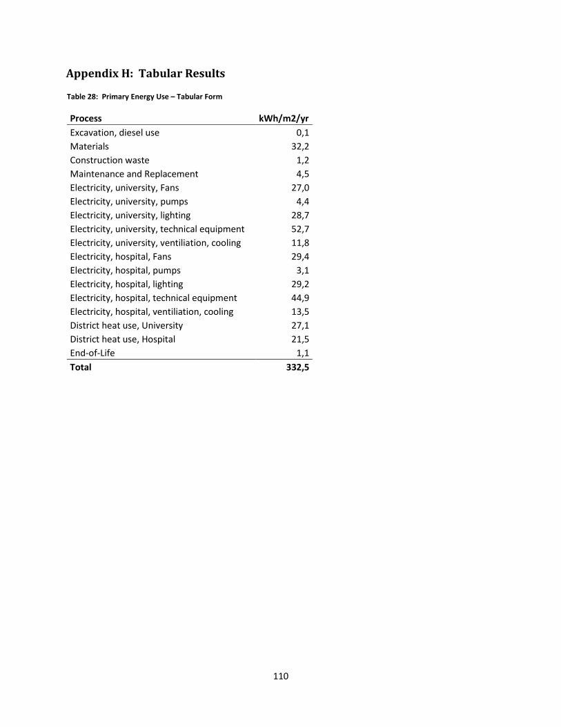
110

Appendix H: Tabular Results

Table 28: Primary Energy Use – Tabular Form

Process kWh/m2/yr Excavation, diesel use 0,1 Materials 32,2 Construction waste 1,2 Maintenance and Replacement 4,5 Electricity, university, Fans 27,0 Electricity, university, pumps 4,4 Electricity, university, lighting 28,7 Electricity, university, technical equipment 52,7 Electricity, university, ventiliation, cooling 11,8 Electricity, hospital, Fans 29,4 Electricity, hospital, pumps 3,1 Electricity, hospital, lighting 29,2 Electricity, hospital, technical equipment 44,9 Electricity, hospital, ventiliation, cooling 13,5 District heat use, University 27,1 District heat use, Hospital 21,5 End-of-Life 1,1 Total 332,5

111

Table 29: Advanced Contribution Analysis – Tabular form

Total Materials

Excavation, diesel use

Construction Waste

Maintenance and Replacement

Electricity, University

Electricity, Hospital

Heat, University

Heat, Hospital End-of-Life

Fossil depletion [kg oil eq/m2/y] 7,70E+00 1,88E+00 1,12E-02 7,61E-02 3,07E-01 2,41E+00 2,32E+00 2,23E-01 3,89E-01 8,95E-02 Metal depletion [kg Fe eq/m2/y] 3,86E+00 1,24E+00 8,58E-04 4,72E-02 6,40E-02 1,26E+00 1,21E+00 1,39E-02 2,42E-02 7,25E-03 Water depletion [m3/m2/y] 4,01E-01 1,09E-01 4,84E-05 4,66E-03 4,91E-03 1,36E-01 1,31E-01 5,97E-03 1,04E-02 6,75E-04 Natural land transformation [m2/m2/y] 5,43E-03 2,03E-03 1,58E-05 8,50E-05 1,47E-04 1,46E-03 1,41E-03 6,13E-05 1,07E-04 1,22E-04 Urban land occupation [m2a/m2/y] 2,83E-01 1,47E-01 6,14E-05 5,87E-03 6,36E-03 5,66E-02 5,45E-02 4,13E-03 7,20E-03 7,14E-04 Agricultural land occupation [m2a/m2/y] 8,11E+00 5,64E+00 9,81E-05 2,41E-01 5,49E-02 9,70E-01 9,35E-01 9,68E-02 1,69E-01 4,87E-04 Marine ecotoxicity [kg 1,4-DB eq/m2/y] 3,25E-01 6,04E-02 5,27E-05 2,33E-03 5,46E-03 7,61E-02 7,34E-02 3,89E-02 6,78E-02 8,98E-04 Freshwater ecotoxicity [kg 1,4-DB eq/m2/y] 3,12E-01 5,60E-02 4,48E-05 2,21E-03 5,61E-03 6,73E-02 6,49E-02 4,20E-02 7,33E-02 9,02E-04 Terrestrial ecotoxicity [kg 1,4-DB eq/m2/y] 2,25E-02 1,61E-03 2,94E-06 6,19E-05 1,85E-04 9,79E-03 9,44E-03 5,23E-04 9,13E-04 2,44E-05 Marine eutrophication [kg N eq/m2/y] 5,15E-03 1,59E-03 1,52E-05 7,18E-05 3,19E-04 1,25E-03 1,20E-03 2,07E-04 3,61E-04 1,25E-04 Freshwater eutrophication [kg P eq/m2/y] 9,25E-03 1,76E-03 1,57E-06 6,31E-05 4,39E-04 3,31E-03 3,19E-03 1,71E-04 2,99E-04 1,50E-05 Terrestrial acidification [kg SO2 eq/m2/y] 9,99E-02 3,33E-02 2,59E-04 1,44E-03 3,49E-03 2,71E-02 2,61E-02 2,28E-03 3,97E-03 2,07E-03 Ionising radiation [kg U235 eq/m2/y] 3,65E+01 1,66E+00 9,23E-04 5,34E-02 1,72E-01 1,71E+01 1,65E+01 3,52E-01 6,13E-01 9,36E-03 Particulate matter formation [kg PM10 eq/m2/y] 5,66E-02 1,66E-02 1,31E-04 8,99E-04 2,11E-03 1,52E-02 1,46E-02 9,51E-04 1,66E-03 4,50E-03 Photochemical oxidant formation [kg NMVOC/m2/y] 8,50E-02 2,75E-02 4,42E-04 1,27E-03 2,76E-03 2,04E-02 1,97E-02 3,43E-03 5,97E-03 3,56E-03 Human toxicity [kg 1,4-DB eq/m2/y] 1,94E+01 3,32E+00 1,76E-03 1,41E-01 3,14E-01 6,41E+00 6,18E+00 1,10E+00 1,91E+00 4,60E-02 Ozone depletion [kg CFC-11 eq/m2/y] 2,12E-06 5,19E-07 3,97E-09 2,03E-08 5,92E-08 6,80E-07 6,55E-07 5,46E-08 9,52E-08 3,18E-08 Climate change [kg CO2 eq/m2/y] 3,36E+01 8,62E+00 3,20E-02 3,04E-01 7,04E-01 9,31E+00 8,98E+00 1,94E+00 3,38E+00 3,04E-01

112