J Grid ComputingDOI 10.1007/s10723-014-9294-7

A Budget Constrained Scheduling Algorithm for WorkflowApplications

Hamid Arabnejad · Jorge G. Barbosa

Received: 18 August 2013 / Accepted: 25 February 2014© Springer Science+Business Media Dordrecht 2014

Abstract Service-oriented computing has enabled anew method of service provisioning based on utilitycomputing models, in which users consume servicesbased on their Quality of Service (QoS) requirements.In such pay-per-use models, users are charged forservices based on their usage and on the fulfilmentof QoS constraints; execution time and cost are twocommon QoS requirements. Therefore, to produceeffective scheduling maps, service pricing must beconsidered while optimising execution performance.In this paper, we propose a Heterogeneous BudgetConstrained Scheduling (HBCS) algorithm that guar-antees an execution cost within the user’s specifiedbudget and that minimises the execution time of theuser’s application. The results presented show that ouralgorithm achieves lower makespans, with a guaran-teed cost per application and with a lower time com-plexity than other budget-constrained state-of-the-artalgorithms. The improvements are particularly highfor more heterogeneous systems, in which a reduc-tion of 30 % in execution time was achieved whilemaintaining the same budget level.

H. Arabnejad · J. G. Barbosa (�)LIACC, Departamento de Engenharia Informatica,Faculdade de Engenharia, Universidade do Porto,Rua Dr. Roberto Frias, 4200-465 Porto, Portugale-mail: jbarbosa@fe.up.pt

H. Arabnejade-mail: hamid.arabnejad@fe.up.pt

Keywords Utility computing · Deadline · Quality ofService · Planning Success Rate

1 Introduction

Utility computing is a service provisioning model thatprovides computing resources and infrastructure man-agement to customers as they need them, as well asa payment model that charges for usage. Recently,service-oriented grid and cloud computing, whichsupply frameworks that allow users to consume util-ity services in a secure, shared, scalable, and standardnetwork environment, have become the basis for pro-viding these services.

Computational grids have been used by researchersfrom various areas of science to execute complex sci-entific applications. Recently, utility computing hasbeen rapidly moving towards a pay-as-you-go model,in which computational resources or services have dif-ferent prices with different performance and Qualityof Service (QoS) levels [3]. In this computing model,users consume services and resources when they needthem and pay only for what they use. Cost and timehave become the two most important user concerns.Thus, the cost/time trade-off problem for schedul-ing workflow applications has become challenging.Scheduling consists of defining an assignment andmapping of the workflow tasks onto resources. In gen-eral, the scheduling problem belongs to a class ofproblems known as NP-complete [8].

H. Arabnejad, J.G. Barbosa

Many complex applications in e-science and e-business can be modelled as workflows [9]. A pop-ular representation of a workflow application is theDirected Acyclic Graph (DAG), in which nodes rep-resent individual application tasks, and the directededges represent inter-task data dependencies. Manyworkflow scheduling algorithms have been developedto execute workflow applications. Some typical work-flow scheduling algorithms were introduced in [24].Most of these algorithms have a single objective, suchas minimising execution time (makespan). However,additional objectives can be considered when schedul-ing workflows onto grids, based on the user’s QoSrequirements. If we consider multiple QoS parame-ters, such as budgets and deadlines, then the problembecomes more challenging.

The contributions of this paper are as follows: a) anew low time complexity algorithm that obtains higherperformance than state-of-the-art algorithms of thesame class for the two set-ups considered here, namelyi) minimising the makespan for a given budget and ii)budget-deadline constrained scheduling; b) a realisticsimulation that considers a bounded multi-port modelin which bandwidth is shared by concurrent communi-cations; and c) results for randomly generated graphs,as well as for real-world applications.

The remainder of the paper is organised as fol-lows. Section 2 describes the system model, includingthe application model, the utility computing model,and the objective function. Section 3 discusses relatedwork on budget-constrained workflow scheduling.The proposed scheduling algorithm (HBCS) is pre-sented in Section 4. Experimental details and sim-ulation results are presented in Section 5. Finally,Section 6 concludes the paper.

2 Problem Definition and System Model

A typical workflow application can be represented bya Directed Acyclic Graph (DAG), which is a directedgraph with no cycles. In a DAG, an individual taskand its dependencies are represented by a node andits edges, respectively. A dependency ensures that achild node cannot be executed before all of its par-ent tasks finish successfully and transfer the inputdata required by the child. The task computation timesand communication times are modelled by assigningweights to nodes and edges respectively. A DAG can

be modelled by a tuple G(N,E), where N is the setof n nodes, each node ni ∈ N represents an appli-cation task, and E is the set of communication edgesbetween tasks. Each edge e(i, j) ∈ E represents atask-dependency constraint such that task ni shouldcomplete its execution before task nj can start.

In a given DAG, a task with no predecessors iscalled an entry task, and a task with no successorsis called an exit task. We assume that the DAG hasexactly one entry task nentry and one exit task nexit . Ifa DAG has multiple entry or exit tasks, a dummy entryor exit task with zero weight and zero communicationedges is added to the graph.

The target utility computing platform is composedof a set of clusters; each cluster has homogeneous pro-cessors that have a given capability and cost to executetasks of a given application. The collection of clustersforms a heterogeneous system. Processors are priced,with the most powerful processor having the highestcost. To normalise diverse price units for the hetero-geneous processors, as defined in [27], the price of aprocessor pj is assumed to be Price(pj ) = αpj

(1 +

αpj)/2, where αpj is the ratio of pj processing capac-

ity to that of the fastest processor. The price will bein the range of ]0 . . . 1], where the fastest proces-sors, with the highest power, have a price value equalto 1.

For each task ni , wi,j gives the estimated time toexecute task ni on processor pj , and Cost (ni , pj ) =wi,j .P rice(pj ) represents the cost of executing taskni on processor pj . After assigning a specific pro-cessor to execute the task ni , AC(ni) is defined asAssigned Cost of task ni . The overall cost for exe-cuting an application is defined as T otalCost =∑

ni∈N AC(ni).The edges of the DAG represent a communica-

tion cost in terms of time, but they are considered tohave zero monetary cost because they occur inside agiven site. The schedule length of a DAG, also calledMakespan, denotes the finish time of the last task inthe scheduled DAG, and is defined by:

makespan = max{AFT (nexit )} (1)

where AFT (nexit ) denotes the Actual Finish Time ofthe exit node. In cases in which there is more thanone exit node, and no redundant node is added, themakespan is the maximum actual finish time of all ofthe exit tasks.

A Budget Constrained Workflow Scheduling Algorithm

The objective of the scheduling problem is to deter-mine an assignment of tasks of a given DAG toprocessors such that the Makespan is minimised, sub-ject to the budget limitation imposed by the user, asexpressed in (2):∑

ni∈NAC(ni) ≤ BUDGET (2)

The user specifies the budget within the rangeprovided by the system, as shown by (3):

BUDGET = CheapestCost

+ kBudget(HighestCost − CheapestCost

)

(3)

where HighestCost and CheapestCost are the costs ofthe assignments produced by an algorithm that guar-antees the minimum processing time, such as HEFT[19], and the least expensive scheduling, respectively.The least expensive assignment is obtained by select-ing the least expensive processor to execute each of theworkflow tasks. The algorithm HEFT is used here asone algorithm that produces the minimum Makespansfor a DAG in a heterogeneous system with complexityO(v2.p) [5]. Therefore, the lower bound of the execu-tion cost is the minimum cost that can be achieved inthe target platform, obtained by the cheapest assign-ment; the upper bound is the cost of the schedulethat produces the minimum Makespan. Finally, thebudget range feasible on the selected platform is pre-sented to the user; he/she selects a budget inside thatrange, represented by kBudget in the range of [0 . . . 1].This budget definition was first introduced by [15].The least expensive assignment guarantees that it isalways feasible to obtain valid mapping within theuser budget, although without guaranteeing the min-imisation of the makespan. If the user can afford topay the highest cost or is limited to the least expensivecost, then the schedule is defined by the HEFT or bythe least expensive assignment, respectively. Betweenthese limits, the algorithm we propose here can beused to produce the assignment.

In conclusion, the scheduling problem described inthis paper is a single objective function, in which onlyprocessing time is optimised, and cost is a problemconstraint, the value of which must be guaranteed bythe scheduler. This feature is very relevant for userswithin the context of the utility computing model,and it is a distinguishing feature compared to otheralgorithms that optimise cost without guaranteeing a

user-defined upper bound, as described in the nextsection.

3 Related Work

Generally, the related research in this area can beclassified into two main categories: QoS optimisationscheduling and QoS constrained scheduling. In thefirst category, the algorithm must find a schedule mapthat optimises all of the QoS parameters to provide asuitable balance between them for time and cost, asin [10, 16–18]. In the second category, the algorithmmakes a scheduling decision to optimise for some QoSparameter while subjected to some user-specified con-straint values. For example, considering budget andmakespan as the QoS parameters, an algorithm inthe first category attempts to find a task-to-processormap that best balances between budget and makespan,while an algorithm of the second category takes user-defined values for the budget as an upper bound anddefines a mapping that optimises the makespan. Thefirst category of algorithms can produce scheduleswith shorter makespans, but the costs of which can-not be limited by the user when submitting the work.Next, we present a review of the second class ofalgorithms.

The Hybrid Cloud Optimised Cost scheduling algo-rithm (HCOC), proposed in [2], and a cost-basedworkflow scheduling algorithm called Deadline-MDP(Markov Decision Process), proposed in [25], addressthe problem of minimising cost while constrained bya deadline. Although these models could have appli-cability in a utility computing paradigm, we do notconsider such a paradigm in this paper.

An Ant Colony Optimisation (ACO) algorithm toschedule large-scale workflows with QoS parameterswas proposed by [7]. Reliability, time, and cost arethree different QoS parameters that are considered inthe algorithm. Users are allowed to define QoS con-straints to guarantee the quality of the schedule. In[14, 21], the Dynamic Constraint Algorithm (DCA)was proposed as an extension of the Multiple-ChoiceKnapsack Problem (MCKP), to optimise two inde-pendent generic criteria for workflows, e.g., executiontime and cost. In [22], a budget constraint workflowscheduling approach was proposed that used geneticalgorithms to optimise workflow execution time whilemeeting the users budget. This solution was extended

H. Arabnejad, J.G. Barbosa

in [23] by introducing a genetic algorithm approachfor constraint-based, two-criteria scheduling (deadlineand budget). In [4], the Balanced Time Scheduling(BTS) algorithm was proposed, which estimates theminimum resource capacity needed to execute a work-flow by a given deadline. The algorithm has somelimitations, such as homogeneity in resource type anda fixed number of computing hosts.

All of the previous algorithms apply guided randomsearches or local search techniques, which require sig-nificantly higher planning costs and thus are naturallytime-consuming. Next, we consider algorithms thatwere proposed for contexts similar to that consideredhere, which are heuristic-based and have lower timecomplexity than the algorithms referred to above andwhich are used in the Results section for comparisonpurposes.

In [15] LOSS and GAIN algorithms were pro-posed to construct a schedule optimising time andconstraining cost. Both algorithms use initial assign-ments made by other heuristic algorithms to meetthe time optimisation objective; a reassignment strat-egy is then implemented to reduce cost and meet thesecond objective, the users budget. In the reassign-ment step, LOSS attempts to reduce the cost, andGAIN attempts to achieve a lower makespan whileattending to the user’s budget limitations. In the initialassignment, LOSS has lower makespans with highercosts, and GAIN has higher makespans with lowercosts. The authors proposed three versions of LOSSand GAIN that differ in the calculation of the tasksweights. The LOSS algorithms obtained better perfor-mance than the GAIN algorithms, and among the threedifferent types of LOSS strategy, we used LOSS1 tocompare to our proposed algorithm. All of the versionsof the LOSS and GAIN algorithms use a search-basedstrategy for reassignments; to obtain their goals, thenumber of iterations needed tends to be high for lowerbudgets in LOSS strategies and for higher budgets inGAIN strategies.

The algorithms LOSS and GAIN differ from ourapproach because they start with a schedule, and thenchanges are made iteratively to the schedule until theuser budget is guaranteed. We do not consider anyinitial schedule, and in contrast to those algorithms,ours is not iterative; the time to produce a schedule isconstant for a given workflow and platform.

A budget-constrained scheduling heuristic calledgreedy time-cost distribution (GreedyTimeCD) was

proposed by [26]. The algorithm distributes the overalluser-defined budget to the tasks, based on the esti-mated tasks average execution costs. The actual costsof allocated tasks and their planned costs are alsocomputed successively at runtime. This is a differentapproach, which optimises task scheduling individu-ally. First, a maximum allowed budget is specifiedfor each task, and a processor is then selected thatminimises time within the task budget.

In [27, 28] the Budget-constrained HeterogeneousEarliest Finish Time (BHEFT) was proposed, whichis an extension of the HEFT algorithm [19]. The con-text of execution is an environment of multiple andheterogeneous service providers; BHEFT defines asuitable plan by minimising the makespan so that theuser’s budget and deadline constraints are met, whileaccounting for the load on each provider. An ade-quate solution is one that satisfies both constraints(i.e., budget and deadline); if no plan can be defined,it is considered a mapping failure. Therefore, the met-ric used by the authors was the planning success rate:the percentage of problems for which a plan wasfound. The BHEFT approach consists of minimis-ing the execution time of a workflow (HEFT based)but within the budget constraints. Our approach isalso one of minimising execution time while beingconstrained to a user-defined budget; therefore, wecompare our proposed algorithm to BHEFT in termsof execution time versus budget. Additionally, wecompare them in terms of plan success rate, wherea deadline is specified for that purpose, similar to[27, 28].

Our algorithm differs from BHEFT in two impor-tant aspects: first, we allow more processors to beconsidered as affordable and, therefore, selected; andsecond, we do not necessarily select the processorthat guarantees the earliest finish time, as BHEFTdoes. Instead, we compute a worthiness value, pro-posed in this paper, which combines the time andcost factors to decide on the processor for the currenttask.

GreedyTimeCD and BHEFT have time complex-ity of O(v2.p) for a workflow of v nodes and aplatform with p processors. Next, we present ourproposed scheduling algorithm, which minimises pro-cessing time while constrained to a user-defined bud-get and with low time complexity and which obtainsbetter schedules then other state-of-the-art algorithms,namely LOSS1, GreedyTimeCD, and BHEFT.

A Budget Constrained Workflow Scheduling Algorithm

4 Proposed Budget Constrained SchedulingAlgorithm

In this section, we present the Heterogeneous Bud-get Constrained Scheduling (HBCS) algorithm, whichminimises execution time while constrained to a user-defined budget. The algorithm starts by computingtwo schedules for the DAG: a schedule that corre-sponds to the minimum execution time that the sched-uler can offer (e.g., produced with HEFT) and thehighest cost; and another schedule that correspondsto the least expensive schedule cost on the targetmachines (CheapestCost ), as explained in Section 2.With the least expensive assignment, the user knowsthe minimum cost and corresponding deadline to exe-cute the job; with the highest cost assignment, the userknows the minimum deadline that can be expected forthe job and the maximum cost that should be spent torun the job. With this information, the user is able toverify whether the platform can execute the job beforethe required deadline and within the associated costrange. If these parameters satisfy the users expecta-tions, he/she specifies the required budget accordingto (3). HBCS is shown in Algorithm 1.

Like most list-based algorithms [12], HBCS con-sists of two phases, namely a task selection phase anda processor selection phase.

4.1 Task Selection

Tasks are selected according to their priorities. Toassign a priority to a task in the DAG, the upwardrank (ranku) [19] is computed. This rank representsthe length of the longest path from task ni to the exitnode, including the computational time of ni , and it isgiven by (4):

ranku(ni) = wi + maxnj∈succ(ni)

{ci,j + ranku(nj )} (4)

where wi is the average execution time of task ni overall of the machines, ci,j is the average communicationtime of an edge e(i, j) that connects task ni to nj overall types of network links in the network, and succ(ni)

is the set of immediate successor tasks to task ni . Toprioritise tasks, it is common to consider average val-ues because they must be assigned a priority beforethe location where they will run is known.

4.2 Processor Selection

The processor selection phase is guided by the fol-lowing quantities related to cost. We define theRemaining Cheapest Budget (RCB) as the remainingCheapestCost for unscheduled tasks, excluding thecurrent task, and the Remaining Budget (RB) as theactual remaining budget. RCB is updated at each stepbefore executing the processor selection block for thecurrent task, using (5) (line 9), which represents thelowest possible cost of the remaining tasks:

Algorithm 1 HBCS algorithm

Require: DAG and user defined BUDGET

1: Schedule DAG with HEFT and Cheapest algo-rithm

2: Set task priorities with ranku3: if HEFTcost < BUDGET

4: return Schedule Map assignment by HEFT5: end if6: RB = BUDGET and RCB = CheapestCost

7: while there is an unscheduled task do8: ni = the next ready task with highest ranku

value9: Update the Remaining Cheapest Budget

(RCB) as defined in Eq.510: for all Processor pi ∈ P do11: calculate FT (ni, pj ) and Cost (ni , pj )

12: end for13: Compute CostCoeff as defined in Eq.714: for all Processor pi ∈ P do15: calculate worthiness(ni , pi) as defined

in Eq.1016: end for17: Psel = Processor pi with highest worthiness

value18: Assign Task ni to Processor Psel

19: Update the Remaining Budget (RB) asdefined in Eq.6

20: end while21: return Schedule Map

RCB = RCB − Costlowest (5)

where Costlowest is the lowest cost for the currenttask among all of the processors. The initial valuefor the Remaining Budget is the user budget (RB =

H. Arabnejad, J.G. Barbosa

BUDGET ), and it is updated with (6) after the pro-cessor selection phase for the current task (line 19).RB represents the budget available for the remainingunscheduled tasks:

RB = RB − Cost (ni , Psel) (6)

where Psel is the processor selected to run the currenttask (line 17 of the algorithm), and Cost (ni , Psel) isthe cost of running task ni on processor Psel .

The quantity Cost Coefficient (CostCoeff ), definedby (7), is the ratio between RCB and RB , and itprovides a measurement of the least expensive assign-ment cost relative to the remaining budget available.If CostCoeff is near one, it means that the availablebudget only allows for selecting the least expensiveprocessors:

CostCoeff = RCB

RB(7)

HBCS minimises execution time. Therefore, thefinish time of the current task (ni ) is computed forall of the processors (FT (ni, pj )) at lines 10 and11, and they constitute one set of factors for proces-sor selection. The other set of factors consists of thecosts of executing the task on each processor, thatis Cost (ni , pj ). The variables pbest and pworst aredefined as the processors with shortest and longestfinish times for the current task, respectively.

Processor selection is based on the combinationof two factors: time and cost. Therefore, we definetwo relative quantities, namely Time rate (T imer ) andCost rate (Costr ), for the current task ni on each pro-cessor pj ∈ P , shown in (8) and (9), respectively:

T imer(ni, pj ) = FTworst − FT (ni, pj )

FTworst − FTbest(8)

Costr (ni , pj ) = Costbest − Cost (ni , pj )

Costhighest − Costlowest

(9)

where FTbest and Costbest are the finish time andcost of the current task on processor pbest , respec-tively. FTworst is the finish time on processor pworst ,and Costhighest and Costlowest are the highest and thelowest cost assignments for the current task among allof the available processors, respectively. T imer mea-sures how much shorter than the worst finish time(FTworst) the finish time is of the current task on pro-cessor pj . Similarly, Costr measures how much lessthe actual cost on pj is than the cost on the processorthat results in the earliest finish time. Both variablesare normalised to their highest ranges.

Finally, to select the processor for the current taskni , the worthiness value for each processor pj ∈ P iscomputed as shown in (10):

worthiness(ni , pi) =

⎧⎪⎪⎪⎪⎪⎪⎪⎪⎨

⎪⎪⎪⎪⎪⎪⎪⎪⎩

−∞ if Cost (ni , pj ) > Costbest

−∞ if Cost (ni , pj ) > RB − RCB

Costr (ni , pj )

.CostCoeff

+T imer(ni, pj ) otherwise

(10)

The first two statements guarantee that if the cost oftask ni on processor pj is higher than the cost on theprocessor that gives the minimum FT and if that cost ishigher than the available budget for task ni , then pro-cessor pj cannot be selected. With these statements,the resulting schedule does not exceed the user budgetand is guaranteed to be valid. In the third statement,the worthiness value depends on the available budgetand on the time during which a processor can finish

the task. If the remaining budget (RB) is high, thenT imer has more influence, and a processor with thegreater difference in FT compared to the worst pro-cessor will have higher worthiness. In contrast, if theremaining budget is smaller, then the cost factor willincrease the worthiness of the processors with lowercost to run task ni . After testing all of the processors,the one with highest worthiness value is selected, andthe remaining budget is updated according to (6).

A Budget Constrained Workflow Scheduling Algorithm

The two phases, task selection and processor selec-tion, are repeated until there are no more tasks remain-ing to schedule. In terms of time complexity, theHBCS requires the computation of HEFT and the leastexpensive schedule, which are used as pre-requisitesto calculate several variables in the HBCS algorithm;these are O(v2.p) and O(v2.p∗), respectively, wherep∗ is the number of cheapest processors. In our plat-form with heterogeneous clusters of homogeneousprocessors, there is more than one processor with thecheapest cost. The least expensive strategy attempts toassign each task to the least expensive processor; con-sidering insertion policy to calculate the Earliest Fin-ish Time (EFT) among all of the cheapest processors,the complexity of the cheapest algorithm is O(v2.p∗).The complexities of the two phases of HBCS are ofthe same order as the HEFT algorithm: O(v2.p). Inconclusion, the total time is O(v2.p+ v2.p∗ + v2.p),which results in time complexity of the orderO(v2.p).

5 Experimental Results

This section presents performance comparisons of theHBCS algorithm with the LOSS1 [15], GreedyTime-CD [26], BHEFT [28], and Cheapest scheduling algo-rithms. We consider synthetic randomly generated andReal Application workflows to evaluate a broaderrange of loads. The results presented were producedwith SimGrid [6], which is one of the best-known sim-ulators for distributed computing and which allows fora realistic description of the infrastructure parameters.

5.1 Workflow Structure

To evaluate the relative performances of the algo-rithms, both the randomly generated and real-worldapplication workflows were used, namely LIGO andEpigenomics [1]. The randomly generated workflowswere created by the synthetic DAG generation pro-gram.1 The computational complexity of a task wasmodelled as one of the three following forms, whichare representative of many common applications: a.d(e.g., image processing of a

√d.√d image), a.dlogd

(e.g., sorting an array of d elements), and d3/2 (e.g.,multiplication of

√d.√d matrices), where a is cho-

sen randomly between 26 and 29. As a result, different

1https://github.com/frs69wq/daggen

tasks exhibit different communication/computationratios.

The DAG generator program defines the DAGshape based on four parameters: width, regularity,density, and jumps. The width determines the maxi-mum number of tasks that can be executed concur-rently. A small value will lead to a thin DAG, similarto a chain, with low task parallelism; a large valueinduces a fat DAG, similar to a fork-join, with a highdegree of parallelism. The regularity indicates the uni-formity of the number of tasks in each level. A lowvalue indicates that the levels contain very dissimilarnumbers of tasks, whereas a high value indicates thatall of the levels contain similar numbers of tasks. Thedensity denotes the number of edges between two lev-els of the DAG, where a low value indicates few edges,and a large value indicates many edges. A jump indi-cates that an edge can go from level l to level l+jump.A jump of one is an ordinary connection between twoconsecutive levels.

In our experiment, for random DAG generation,we used as the number of tasks n = [10...60],jump = [1, 2, 3], regularity = [0.2, 0.4, 0.8],f at = [0.2, 0.4, 0.8], and density = [0.2, 0.4, 0.8].With these parameters, each DAG was created bychoosing the value for each parameter randomly fromthe parameter data set. The total number of DAGsgenerated in our simulation was 1000.

5.2 Simulation Platform

We resorted to simulation to evaluate the algorithmsdiscussed in the previous sections. Simulation allowsus to perform a statistically significant number ofexperiments for a wide range of application config-urations in a reasonable amount of time. We usedthe SimGrid toolkit2 [6] as the basis for our sim-ulator. SimGrid provides the required fundamentalabstractions for the discrete-event simulation of par-allel applications in distributed environments. It wasspecifically designed for the evaluation of schedul-ing algorithms. Relying on a well-established simu-lation toolkit allows us to leverage sound models ofa heterogeneous computing system, such as the gridplatform considered in this work. In many researchpapers on scheduling, the authors have assumed acontention-free network model, in which processors

2http://simgrid.gforge.inria.fr

H. Arabnejad, J.G. Barbosa

Table 1 Description of theGrid5000 clusters fromwhich the platforms used inthe experiments werederived

Site Cluster #CPUT otal #CPUused Power(GFlop/s) σ

Lille chicon 26 2 4 9 8.9618

chimint 20 2 4 7 23.531 0.69

chinqchint 46 4 8 16 22.270

Sophia helios 56 3 6 12 7.7318

sol 50 3 5 10 8.9388 0.90

suno 45 2 5 10 23.530

can simultaneously send data to or receive data fromas many processors as possible, without experienc-ing any performance degradation. Unfortunately, thatmodel, the multi-port model, is not representative ofactual network infrastructures. Conversely, the net-work model provided by SimGrid corresponds to atheoretical bounded multi-port model. In this model,

a processor can communicate with several other pro-cessors simultaneously, but each communication flowis limited by the bandwidth of the traversed route, andcommunications using a common network link mustshare bandwidth. This scheme corresponds well to thebehaviour of TCP connections on a LAN. The validityof this network model was demonstrated by [20].

Fig. 1 NormalizedMakespan for Randomworkflows with CPUused=8

A Budget Constrained Workflow Scheduling Algorithm

We consider two sites that comprise multipleclusters. Table 1 provides the name of each clus-ter, along with its number of processors, processingspeed expressed in GFlop/s, and the standard devia-tion (σ ) of CPU capacity as a heterogeneity factor.Column #CPUused shows the number of processorsused from each cluster for 8-, 16- and 32-processorconfigurations.

5.3 Budget-Deadline Constrained Scheduling

Budget-deadline constrained scheduling was intro-duced in [27, 28], in which the BHEFT algorithmwas presented. Its aim is to produce mappings oftasks to resources that meet the deadline and bud-get constraints imposed by the user. Although BHEFT

considers the load of the providers, the algorithm canbe evaluated by attending exclusively to the dead-line and budget constraints and ignoring the providersloads, as also presented in [27, 28]. This processallows for evaluating and comparing the algorithms,without the additional random variables that are theproviders loads. The budget factor is considered here,as defined by (3). The deadline constraint is definedby (11), which specifies a deadline value for a givenworkflow, based on the mapping obtained by HEFT:

DeadLine = LBdeadline

+ kDeadline

(UBdeadline − LBdeadline

)

(11)where LBdeadline is equal to HEFTMakespan, themakespan obtained with HEFT, and UBdeadline is

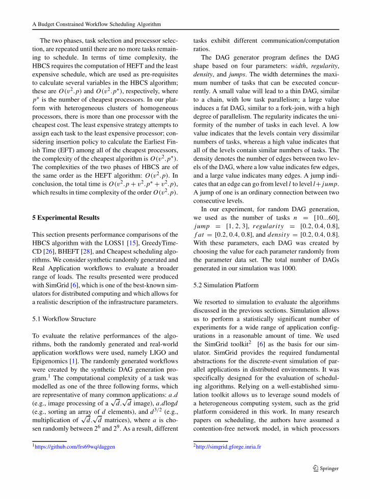
Fig. 2 NormalizedMakespan for Randomworkflows withCPUused=32

H. Arabnejad, J.G. Barbosa

3.HEFTMakespan. The range of values for kDeadline

is [0 . . .1]. HEFTMakespan is the minimum time thatthe user is allowed to choose to obtain a valid sched-ule. We restrict the upper bound deadline as the cubeof HEFTMakespan to evince the quality of the algo-rithms in generating valid mappings.

5.4 Performance Metrics

To evaluate and compare our algorithm with otherapproaches, we consider the metric NormalisedMakespan (NM), defined by (12). NM normalises themakespan of a given workflow to the lower bound,which is the workflow execution time obtained withHEFT:

NM = schedule makespan

HEFTMakespan

(12)

To evaluate the algorithms using the budget-deadline constrained methodology, we consider thePlanning Success Rate (PSR), as expressed by (13)and defined in [27, 28]. This metric provides thepercentage of valid schedules obtained in a givenexperiment.

PSR = 100 × Successful Planning

Total Number in experiment(13)

5.5 Results and Discussion

Among all of the algorithms mentioned abovein the related work section, we selected LOSS1,GreedyTimeCD, BHEFT, and Cheapest schedulingalgorithms; these match our goal and conditions, butwe have made some modifications in their original

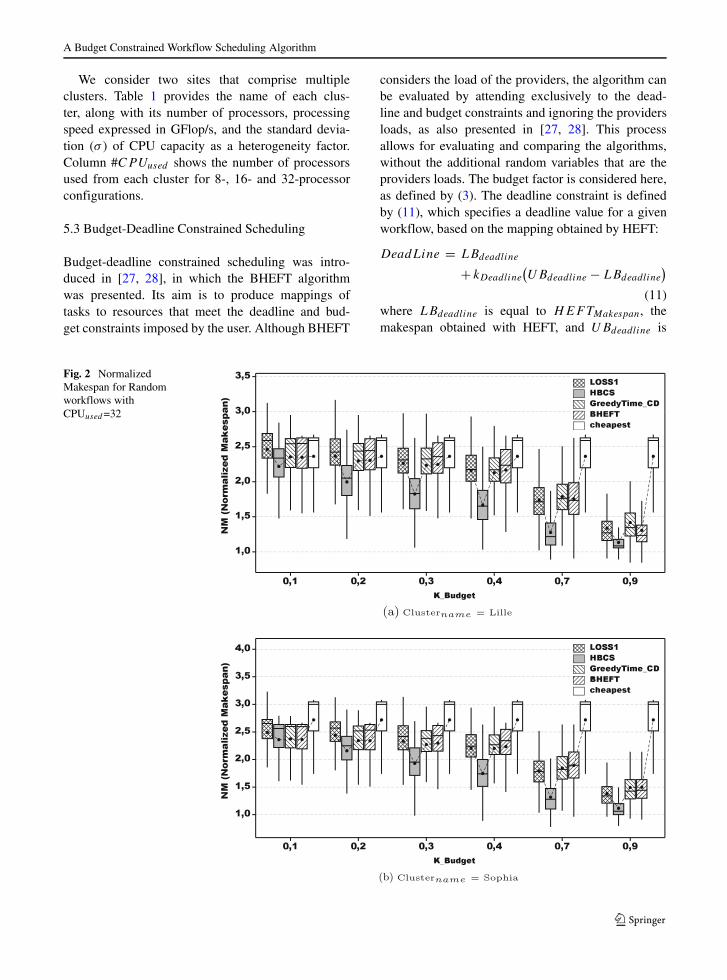
Fig. 3 Planning SuccessRate for Random workflows

A Budget Constrained Workflow Scheduling Algorithm

strategies. The original implementation of the LOSSscheduling algorithm assumed that all of the pro-cessors had different costs, and therefore, there wasno conflict in selecting a processor based on thecost parameter. In our grid environment, each clus-ter was homogeneous and was based only on the costparameter, so there could be more than one processorcandidate. In this case, we tested all of the possibleprocessors and selected that which achieved the small-est makespan. The same procedure was applied to theleast expensive scheduling strategy, which attemptsto schedule each task on the service with the lowerexecution cost.

To evaluate the performance of each algorithm, wecomputed the makespan for each DAG and normalisedit using (12). The results presented next were obtainedby SimGrid with the bounded multi-port model, andthey are presented for two data sets: randomly gener-ated workflows and real applications.

5.5.1 Results for Randomly Generated Workflows

For random DAG generation, as stated previously,we model the computational complexity of commonapplications tasks, such as image processing, arraysorting, and matrix multiplication. Figures 1 and 2show the Normalised Makespan values obtained ontwo CPU configurations per site, namely, 8 and 32processors. We can see that the HBCS algorithmobtains significant performance improvements overthe other algorithms for most of the user-defined bud-get values and configurations. For 8 processors on theLille site, the improvement of HBCS over BHEFT is2.0 % for k = 0.1, and it increases to 19.7 % fork = 0.9. On the Sophia site, the improvement is 0 %for k = 0.1, and it increases to 29.4 % for k = 0.9.For k ≥ 0.7, the second-best algorithm is LOSS1, andthe improvements of HBCS over LOSS1 are 24.7 %and 18.2 % for k = 0.7 and k = 0.9, respectively.

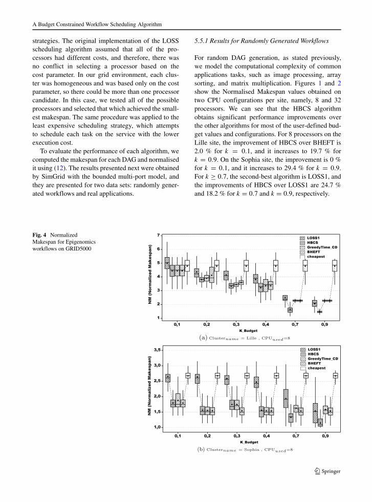
Fig. 4 NormalizedMakespan for Epigenomicsworkflows on GRID5000

H. Arabnejad, J.G. Barbosa

Fig. 5 NormalizedMakespan for LIGOworkflows on GRID5000

For 32 processors, the same pattern of results isobtained on the Lille and Sophia sites but with greaterdifferences for lower k values. On the Lille site, theimprovement of HBCS over BHEFT is 5.4 %, 13.4 %and 18.8 % for k values of 0.1, 0.2, and 0.3, respec-tively. The performance of BHEFT and GreedyTime-CD are very similar for all of the ranges of k on bothsites. For k ≥ 0.7, the second best algorithm is againLOSS1.

In conclusion, HBCS outperforms all of the otheralgorithms, indicating that HBCS can achieve lowermakespans for any given budget.

The results of the evaluation made with the budget-deadline constrained methodology are shown in Fig. 3,where the deadline and budget factors assume the val-ues of 0.2, 0.5, and 0.8. The figures present the averagevalues for 8, 16 and 32 processors for each site. HBCSyielded higher PSR values for all of the cases. ThePSR obtained by HBCS for shorter deadline factors issignificantly higher than the PSR values obtained withthe other algorithms. On both sites, for deadline and

budget factors of 0.2 and 0.8, respectively, the HBCSPSR is greater than 80 %, while for the remainingalgorithms, the PSR is less than 30 %. We can con-clude that HBCS obtains the highest Planning SuccessRates for the two levels of heterogeneity consideredhere.

5.5.2 Results for Real World Applications

To evaluate the algorithms on a standard and real setof workflow applications, synthetic workflows weregenerated using the code developed in [13]. Two well-known structures were chosen [11], namely Epige-nomics,3 for mapping the epigenetic state of humanDNA, and LIGO.4 The Epigenomics workflow is ahighly pipelined application with multiple pipelinesoperating on independent chunks of data in parallel. In

3USC Epigenome Center, http://epigenome.usc.edu4http://www.advancedligo.mit.edu

A Budget Constrained Workflow Scheduling Algorithm

these two real applications, most of the jobs have highCPU utilisation and relatively low I/O, so they can beclassified as CPU-bound workflows.

Workflows with 24 and 30 tasks were createdfor both Epigenomics and LIGO. For each workflowsize, 300 different workflow instances were generated,obtaining a total collection of 600 workflows for eachtype of application.

For Normalised Makespan, Figs. 4 and 5 show thatHBCS achieves better performance for most of thebudget factor values. The improvements increase withthe budget factor and the site heterogeneity. Similarbehaviour is obtained for the LIGO application.

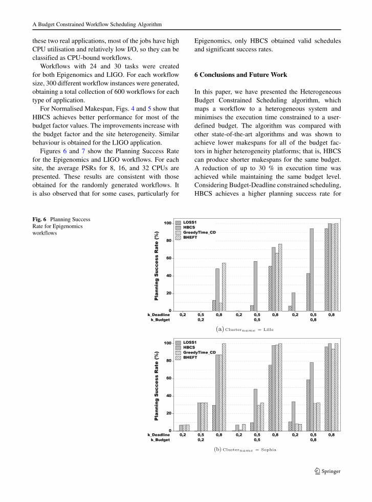
Figures 6 and 7 show the Planning Success Ratefor the Epigenomics and LIGO workflows. For eachsite, the average PSRs for 8, 16, and 32 CPUs arepresented. These results are consistent with thoseobtained for the randomly generated workflows. Itis also observed that for some cases, particularly for

Epigenomics, only HBCS obtained valid schedulesand significant success rates.

6 Conclusions and Future Work

In this paper, we have presented the HeterogeneousBudget Constrained Scheduling algorithm, whichmaps a workflow to a heterogeneous system andminimises the execution time constrained to a user-defined budget. The algorithm was compared withother state-of-the-art algorithms and was shown toachieve lower makespans for all of the budget fac-tors in higher heterogeneity platforms; that is, HBCScan produce shorter makespans for the same budget.A reduction of up to 30 % in execution time wasachieved while maintaining the same budget level.Considering Budget-Deadline constrained scheduling,HBCS achieves a higher planning success rate for

Fig. 6 Planning SuccessRate for Epigenomicsworkflows

H. Arabnejad, J.G. Barbosa

Fig. 7 Planning SuccessRate for LIGO workflows

more heterogeneous systems. In some particular cases,the PSR obtained with HBCS is considerably higherthan the PSRs obtained with the other algorithms. Forexample, for the budget and deadline factors of 0.8and 0.2, respectively, on the Lille and Sophia sites,the PSR of HBCS is greater than 80 %, while all ofthe other algorithms achieve PSRs less than 30 %. Onthese sites, HBCS performs significantly better thanthe other algorithms for the more restricted deadlinefactors of 0.2 and 0.5.

The results achieved for two real applications,namely LIGO and Epigenomics, are consistent withthe randomly generated workflows for both metrics.

Concerning time complexity, HBCS has the samecomplexity as GreedyTimeCD and BHEFT, having aconstant running time for all ranges of budget fac-tors for a given workflow and platform, because ithas bounded complexity. In contrast, the LOSS algo-rithms have a search-based step, and their runningtime therefore depends on the number of iterations to

find a solution, where for lower budgets, the numberof iterations is significantly greater.

In conclusion, we have presented the HBCS algo-rithm for budget constrained scheduling, which hasproved to achieve better performance with lower timecomplexity than other state-of-the-art algorithms. Theresults were obtained in a simulation with a realis-tic model of the computing platform and with sharedlinks, as occurs in a common grid infrastructure.

In future work, we intend to extend the algorithmto consider the dynamic concurrent DAG schedulingproblem. This consideration will allow users to exe-cute concurrent workflows that might not be able tostart together but that can share resources so that thetotal cost for the user can be minimised.

Acknowledgments This work was supported in part by theFundacao para a Ciencia e Tecnologia, PhD Grant FCT - DFRH- SFRH/BD/80061/2011.

A Budget Constrained Workflow Scheduling Algorithm

References

1. Bharathi, S., Chervenak, A., Deelman, E., Mehta, G., Su,M.H., Vahi, K.: Characterization of scientific workflows.In: Third Workshop on Workflows in Support of Large-Scale Science, 2008. WORKS 2008, pp. 1–10. IEEE (2008)

2. Bittencourt, L.F., Madeira, E.R.M.: Hcoc: a cost optimiza-tion algorithm for workflow scheduling in hybrid clouds. J.Internet Serv. Appl. 2(3), 207–227 (2011)

3. Broberg, J., Venugopal, S., Buyya, R.: Market-orientedgrids and utility computing: The state-of-the-art and futuredirections. J. Grid Comput. 6(3), 255–276 (2008)

4. Byun, E.-K., Kee, Y.-S., Kim, J.-S., Deelman, E., Maeng,S.: Bts: Resource capacity estimate for time-targeted sci-ence workflows. J. Parallel Dist. Comput. 71(6), 848–862(2011)

5. Canon, L.C., Jeannot, E., Sakellariou, R., Zheng, W.: Com-parative evaluation of the robustness of dag schedulingheuristics. In: Grid Computing, pp. 73–84. Springer (2008)

6. Casanova, H., Legrand, A., Quinson, M.: Simgrid: a genericframework for large-scale distributed experiments. In: Pro-ceedings of the Tenth International Conference on Com-puter Modeling and Simulation, UKSIM ’08, pp. 126–131.IEEE Computer Society, Washington (2008)

7. Chen, W.-N., Zhang, J.: An ant colony optimizationapproach to a grid workflow scheduling problem with vari-ous qos requirements. IEEE Trans. Syst. Man Cybern. PartC Appl. Rev. 39(1), 29–43 (2009)

8. Coffman, E.G., Bruno, J.L.: Computer and Job-shopScheduling Theory. Wiley (1976)

9. Deelman, E., Blythe, J., Gil, Y., Kesselman, C., Mehta,G., Vahi, K., Blackburn, K., Lazzarini, A., Arbree, A.,Cavanaugh, R., et al: Mapping abstract complex workflowsonto grid environments. J. Grid Comput. 1(1), 25–39 (2003)

10. Dogan, A., Ozguner, F.: Bi-objective scheduling algorithmsfor execution time–reliability trade-off in heterogeneouscomputing systems. Comput. J. 48(3), 300–314 (2005)

11. Juve, G., Chervenak, A., Deelman, E., Bharathi, S., Mehta,G., Vahi, K.: Characterizing and profiling scientific work-flows. Futur. Gener. Comput. Syst. 29(3), 682–692 (2013)

12. Kwok, Y., Ahmad, I.: Static scheduling algorithms forallocating directed task graphs to multiprocessors. ACMComput. Surv. 31(4), 406–471 (1999)

13. Pegasus. Pegasus workflow generator. https://confluence.pegasus.isi.edu/display/pegasus/WorkflowGenerator(2013)

14. Prodan, R., Wieczorek, M.: Bi-criteria scheduling of scien-tific grid workflows. IEEE Trans. Autom. Sci. Eng. 7(2),364–376 (2010)

15. Sakellariou, R., Zhao, H., Tsiakkouri, E., Dikaiakos, M.:Scheduling workflows with budget constraints. Integr. Res.Grid Comput., 189–202 (2007)

16. Singh, G., Kesselman, C., Deelman, E.: A provisioningmodel and its comparison with best-effort for performance-cost optimization in grids. In: Proceedings of the 16thInternational Symposium on High Performance DistributedComputing, pp. 117–126. ACM (2007)

17. Sen, S., Li, J., Qingjia, H., Shuang, K., Wang, J.: Cost-efficient task scheduling for executing large programs in thecloud. Parallel Comput. 39, 177–188 (2013)

18. Szabo, C., Kroeger, T.: Evolving multi-objective strate-gies for task allocation of scientific workflows on publicclouds. In: WCCI IEEE World Congress on ComputationalIntelligence, pp. 1–8. IEEE (2012)

19. Topcuoglu, H., Hariri, S., Wu, M.: Performance-effectiveand low-complexity task scheduling for heterogeneouscomputing. IEEE Trans. Parallel Distrib. Syst. 13(3), 260–274 (2002)

20. Velho, P., Legrand, A.: Accuracy study and improve-ment of network simulation in the simGrid framework. In:Proccedings of the 2nd International Conference on Sim-ulation Tools and Techniques (SIMUTools). Rome, Italy(2009)

21. Wieczorek, M., Podlipnig, S., Prodan, R., Fahringer, T.:Bi-criteria scheduling of scientific workflows for the grid.In: 8th IEEE International Symposium on Cluster Com-puting and the Grid, 2008. CCGRID’08, pp. 9–16. IEEE(2008)

22. Yu, J., Buyya, R.: A budget constrained schedulingof workflow applications on utility grids using geneticalgorithms. In: Workshop on Workflows in Support ofLarge-Scale Science, 2006. WORKS’06, pp. 1–10. IEEE(2006)

23. Yu, J., Buyya, R.: Scheduling scientific workflow appli-cations with deadline and budget constraints using geneticalgorithms. Sci. Program. 14(3), 217–230 (2006)

24. Yu, J., Buyya, R., Ramamohanarao, K.: Workflow schedul-ing algorithms for grid computing. Metaheuristics Sched.Distrib. Comput. Environ., 173–214 (2008)

25. Yu, J., Buyya, R., Tham, C.K.: Cost-based scheduling ofscientific workflow applications on utility grids. In: FirstInternational Conference on e-Science and Grid Comput-ing, 2005, pp. 8–pp. IEEE (2005)

26. Jia, Y., Ramamohanarao, K., Buyya, R.: Deadline/budget-based scheduling of workflows on utility grids. Market-Oriented Grid Util. Comput., 427–450 (2009)

27. Zheng, W., Sakellariou, R.: Budget-deadline con-strained workflow planning for admission control inmarket-oriented environments. In: Economics of Grids,Clouds, Systems, and Services, pp. 105–119. Springer(2012)

28. Zheng, W., Sakellariou, R.: Budget-deadline constrainedworkflow planning for admission control. J. Grid Comput.,1–19 (2013)