A Brief Introduction to Vehicle Dynamics

Presented by: William BombardierTeam Captain Mini Baja 2007

May 16th 2006

Outline of Presentation

Tires BehaviorLongitudinal DynamicsLateral (Handling) DynamicsVertical Dynamics (Suspension)Suspension Kinematics (Elastokinematics)

Tire Behavior

http://www.easterntireinc.com/graphics/tires1.jpg

The tire itself is highly non-linear and it is extremely difficult to model.• Inflated (it’s essentially a pressure

vessel)• Contact stresses (tires deflect a

lot when they roll)• Rotating effects (tire diameter

increases with speed)• Large deflections • Non-linear material properties

There exists two types of tires.• Radial tires

• Bias-Ply tires

http://www.bartleby.com/images/A4images/A4biaspl.jpghttp://www.tireguides.com/images/highperformanceradial.jpg

The difference between the two types of tires is the orientation of the fibres, and the angle at which the cords lie determine the stiffness of the tire in cornering.

Tire BehaviorThe acts like a spring in the vertical direction. The stiffness of the tire changes with inflation pressure and tire deflection.

δ

F

Increasing inflation Pressure

The stiffness of the tire is typically in the range of 150-250 kN/m, the tire stiffness is typically 10 times the suspension stiffness.The deformation in the tire as it rolls leads to energy loss, and therefore rolling resistance (an effect denoted the hysterisis effect).

http://www.doitpoms.ac.uk/tlplib-dev/bioelasticity/images/img025.gifhttp://images.google.ca/imgres?imgurl=http://webphysics.davidson.edu/faculty/dmb/PY430/Friction/idealroll1.gif&imgrefurl=http://webphysics.davidson.edu/faculty/dmb/PY430/Friction/rolling.html&h=303&w=418&sz=13&tbnid=6u84OCzRccuMzM:&tbnh=88&tbnw=122&hl=en&start=2&prev=/images%3Fq%3Dtire%2Bfriction%2Brolling%26svnum%3D10%26hl%3Den%26lr%3D

Tire Behavior

( )( )ZRR FKF =The rolling losses are usually represented by a rolling loss factor.

Vehicle Speed

Rolling loss factor (KR)

0.01

0.015

As a result, the forward speed and the rotational speed are not related by the physical radius of the tire, but by an effective rolling radius.

( )( )erv ϖ=

Tire Behavior1

0−=

ϖωσ

z

x

FF

=µ

As the tire provides force in traction or braking it must slip relative to the road.

Tire BehaviorThe tire also slips in the lateral direction.

http://www.donpalmer.co.uk/cchandbook/images/tyrebasics.gif

Tire BehaviorThe tire also slips in the lateral direction.

http://code.eng.buffalo.edu/dat/sites/tire/img54.gif

Tire BehaviorThe lateral load increases with increasing normal load, but at adecreasing rate ie: µ decreases with load. It is this behavior that allows us to use suspension stiffness to adjust oversteer/understeerbehavior.

Fz

Fy

Increasing tire slip angle (α)

As the vehicle corners, there will be weight transfer from the inner to the outer tire. The normal load will shift from the N+∆N on the outer more loaded tire, and from N-∆N on the inner less loaded tire.

FzN+∆N N-∆N N

FyThe lateral force capability at the inner tire is decreased, and the lateral force capability of the outer tire is increased, but not as much. The result is a net loss in grip capabilities

Tire BehaviorThe load transfer across either the front or the rear axle depends on the relative roll stiffness of the suspension. If the front suspension of the vehicle is stiffer in roll than the rear suspension, the front axle will experience a larger weight transfer ∆N than the rear axle. The front axle will then experience a larger decrease in grip capabilities than the rear, and the result is that the front axle will need to operate at larger slip angles, and the vehicle will understeer.As the lateral loads are developed in the contact patch, the distribution tends to be asymmetric (as previously noted for the longitudinalforces) and a self aligning moment is created.

Mz

α

Increasing N

Tire BehaviorIf it is desired to model both the longitudinal force and the lateral force simultaneously we will need a coupled tire model, as the two forces will be related. The total friction force at the tire must fall inside the “friction circle”.

As the traction or braking forces increase the maximum lateral force must decrease.

12

max

2

max≤⎟⎟

⎠

⎞⎜⎜⎝

⎛+⎟⎟

⎠

⎞⎜⎜⎝

⎛y

y

x

x

µµ

µµ

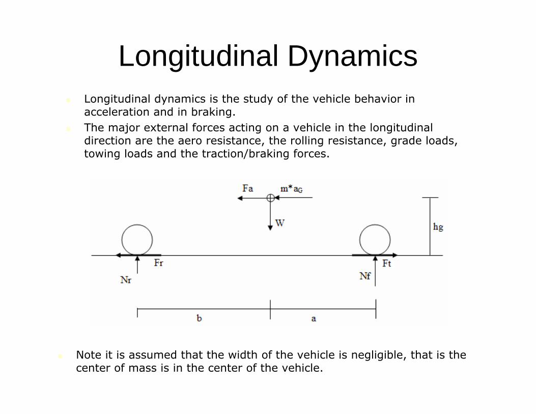
Longitudinal DynamicsLongitudinal dynamics is the study of the vehicle behavior in acceleration and in braking.The major external forces acting on a vehicle in the longitudinal direction are the aero resistance, the rolling resistance, grade loads, towing loads and the traction/braking forces.

Note it is assumed that the width of the vehicle is negligible, that is the center of mass is in the center of the vehicle.

Longitudinal DynamicsAerodynamic forces

2

21 AuCF daa ρ=

• The aerodynamic resistance is generated from two sources, air flow over/around the vehicle and cooling/ventilation

90% do to air flow81% do to pressure drag9% do to skin friction

Traction ForcesThere are two limiting factors that determine the performance of a road vehicle, the traction force that the tire can support, and the force that the engine/transmission can produce.• Typically in low gears with large throttle openings the traction force is

limited by tire, but usually determined by the engine.

The internal combustion engine starts operation at relatively low speed but produces its best torque at intermediate speed ranges.A transmission is required to:• Achieve appropriate engine speed to vehicle speed ratio• Allow smooth starts, even on hills• Match engine characteristics for maximum fuel economy

Longitudinal DynamicsTypical Power and Torque curves of an IC engine

Longitudinal DynamicsTransmission Ratios• Typically, the higher gear ratios are chosen to match the designed vehicle

speed with an appropriate engine speed. The lower ratios are selected for torque requirements (to ensure that the vehicle has enough force to overcome grades in low speeds)

Equation to calculate the vehicle speed

( )( )( )( )( )axn

le ruεε

σω −=

1

Equation to calculate the traction force

( )( )( )l

tnaxet

rTF ηεε

=

Equation to calculate the percent of the grade

( )°=

=45%100

%tan100grade

gradeθ

Longitudinal DynamicsTypical traction force vs. vehicle speed curve

Longitudinal DynamicsThe ideal tire curve

σ

Ft

ftmax

For passenger cars, the ratios generally do not follow a geometric progression, but rather are spaced further apart at lower gears, and closer together at higher gears; this improves the acceleration performance of the vehicle.When a vehicle is accelerating (braking) there is load transfer from the front of the vehicle to the rear (from the rear to the front).

( ) Gmaba

hN+

=∆

Longitudinal Dynamics

( )( )( )( )( )( )g

thl

agmFµ

µ−

=max

( ) ( ) hbaa

µµθ−+

=tan

Since the tire is slipping relative to the road, there is a maximum traction force that the vehicle can produce.

(rear wheel drive)

The maximum grade that a vehicle can climb is determined by considering both the max. grade before traction is lost, and themaximum grade that can be climb at maximum engine torque.

( )r

tmg axne ηεεθ maxsin =

Longitudinal Dynamics

gaG µ=max

NNF

f

ff

∆+=µ

Braking forcesThe maximum (ideal situation) amount of deceleration occurs when all four tires lock simultaneously

Define the effective coefficient at the front and rear axle

NNF

r

rr

∆−=µ

By using the effective coefficient of frictions and setting them equal to each other the equation that defines the curve which allows all four tires to lock simultaneously can be determined.

( ) ( ) 02 =−++ aFbFh

mgFF frrf

Longitudinal Dynamics

In actual vehicles the curve is not parabolic it is a straight line. That is the force at the front tire is linearly related to the force at the rear tire.It is important that the front wheels lock before the rear wheels, because if the rear wheels lock first the vehicle will be unstable in yaw.

Longitudinal DynamicsThe ideal situation would be to use a pressure proportioning valve to ensure that the front tires lock first.

Ff

Fr

optimal

actual

Handling (Lateral) DynamicsThe handling dynamics of a road vehicle are described by a single dynamic model, the bicycle model.

( ) ( )

( ) ( ) δ⎭⎬⎫

⎩⎨⎧

=⎭⎬⎫

⎩⎨⎧

⎥⎥⎥⎥

⎦

⎤

⎢⎢⎢⎢

⎣

⎡

+−

+−+

+⎭⎬⎫

⎩⎨⎧⎥⎦

⎤⎢⎣

⎡f

f

rfrf

rfrf

aCC

rv

uCbCa

ubCaC

muu

bCaCu

CC

rv

Im

2200

&

&

It is important to note that the longitudinal effects are not considered in the handling analysisThe assumptions in the linear bicycle model:• The tires on either side of the vehicle have the same effect on the dynamics• The width of the vehicle is assumed to be constant• The forward speed of the vehicle is fixed• Small slip angles at each of the tires• Bounce and pitch motions are negligible• Linear tire force/slip angle relationship

Handling (Lateral) Dynamics

( ) ( )( ) rf

rf

CCbabCaCmuba

ur

+−

−+= 2δ

ruR =

Using the bicycle model allows the effects of various design parameters on vehicle handling with relative ease. These include:• Steady state effects• Transient effects• Frequency input effects

Steady state effects:

( ) ( )

( ) ( ) δ⎭⎬⎫

⎩⎨⎧

=⎭⎬⎫

⎩⎨⎧

⎥⎥⎥⎥

⎦

⎤

⎢⎢⎢⎢

⎣

⎡

+−

+−+

f

f

rfrf

rfrf

aCC

rv

uCbCa

ubCaC

muu

bCaCu

CC

22

From the steady state equation we can obtain the following equations that describe the vehicle in handling dynamics:

( )( ) rf

rf

o CCbabCaCmu

RR

2

2

1+

−−=

Handling (Lateral) Dynamics

( )uv

=βtan ( )( ) ( )

( ) rf

rf

r

CCbabCaCmuba

Cbaamub

+−

−+

+−

= 2

2

δβ

From the steady state equation we can obtain the following equations that describe the vehicle in handling dynamics:

Consider the concepts of oversteer, understeer, and neutral steer• A vehicle oversteers when the actual cornering radius decreases with vehicle

speed (aCf<bCr).• A vehicle understeers when the radius of the path increases with vehicle

speed (aCf=bCr).• A vehicle neutral steers when the radius of curvature is independent of

vehicle speed (aCf>bCr).

Handling (Lateral) Dynamics

rf

f

bCaCaC−

=δβ

( )rf

rfcritical

bCaCmbaCCu

−+

=2)(

Important notes:• At low speeds, the (β/δ) ratio is positive, indicating that the rear of the

vehicle tracks inside the front.• At high speeds, the rear of the vehicle will eventually begin to track outside

the front. • For an understeering vehicle the (β/δ) ratio tends to a limit:

• For an oversteering vehicle the (β/δ) tends to infinity at the critical speed:

• The (r/δ) ratio tends to infinity at the critical speed for an oversteeringvehicle, and for an understeering vehicle it is a maximum at the characteristic speed.

( )fr

rfsticcharacteri

aCbCmbaCCu

−+

=2)(

Handling (Lateral) DynamicsTransient Effects

( ) ( )

( ) ( ) 00

022 =

⎭⎬⎫

⎩⎨⎧

⎥⎥⎥⎥

⎦

⎤

⎢⎢⎢⎢

⎣

⎡

+−

+−+

+⎭⎬⎫

⎩⎨⎧⎥⎦

⎤⎢⎣

⎡rv

uCbCa

ubCaC

muu

bCaCu

CC

rv

Im

rfrf

rfrf

&

&

( ) ( )( ) ( )

AACBBs

bCaCmuCCbaC

CCIuCbCamuBmIuA

rfrf

rfrf

242

22

22

2

−±−=

−−+=

+++=

=

If s is negative the vehicle is always stable, and if s is positive the vehicle is not stable. A vehicle is always stable if it is an understeeringvehicle, and the vehicle will become unstable at the critical speed if it is an oversteering vehicle.

Handling (Lateral) DynamicsSteering frequency input

( ) ( )

( ) ( )

st

f

f

rfrf

rfrf

e

aCC

rv

uCbCa

ubCaC

muu

bCaCu

CC

rv

Im

∆=

⎭⎬⎫

⎩⎨⎧

=⎭⎬⎫

⎩⎨⎧

⎥⎥⎥⎥

⎦

⎤

⎢⎢⎢⎢

⎣

⎡

+−

+−+

+⎭⎬⎫

⎩⎨⎧⎥⎦

⎤⎢⎣

⎡

δ

δ2200

&

&

Usually it is of more interest to find the response of the vehicle to general steer input (δ = δ(t)). The bicycle model can then be used to calculate the yaw rate and the lateral velocity by using numerical methods. Given constants u, v, and r as functions of time, the x, y, and θ of the vehicle can also be found.

( ) ( )( ) ( )θθ

θθθ

cossinsincos

vuyvux

r

−=+=

−=

&

&

&

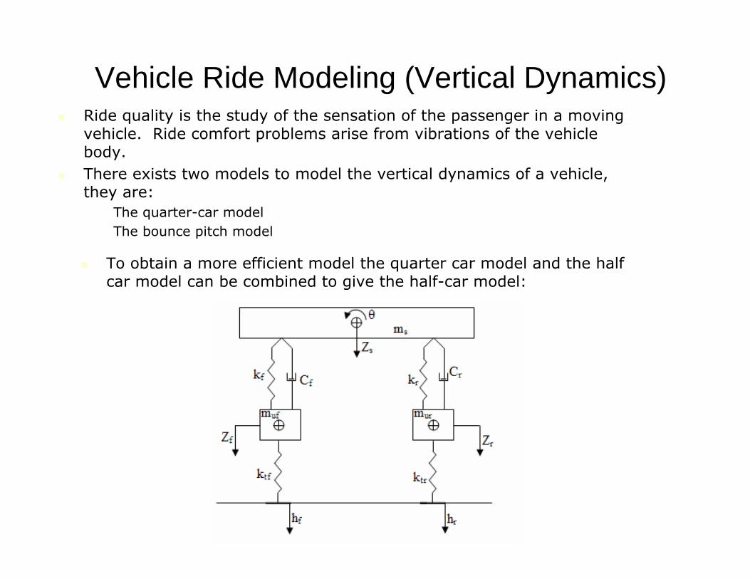
Vehicle Ride Modeling (Vertical Dynamics)Ride quality is the study of the sensation of the passenger in a moving vehicle. Ride comfort problems arise from vibrations of the vehicle body.There exists two models to model the vertical dynamics of a vehicle, they are:• The quarter-car model• The bounce pitch model

To obtain a more efficient model the quarter car model and the half car model can be combined to give the half-car model:

Vehicle Ride Modeling (Vertical Dynamics)The quarter car model:

AACBB

AACBB

kkCkmkmkmB

mmA

ts

sutsss

us

24

24

22

2

22

1

−+=

−−=

=+=

=+

ϖ

ϖ

For typical passenger vehicles the sprung mass is roughly one order of magnitude higher than the unsprung mass (ms=10mu)Also the stiffness of the tire is typically an order of magnitude higher than the suspension stiffness.

kt = 150-200kN/mks = 20kN/m

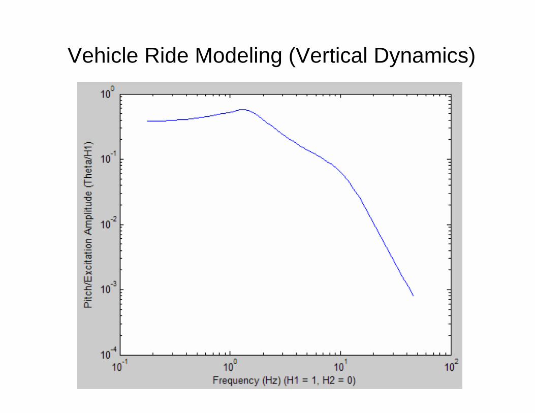
The frequencies are typically in the range of 1-1.5Hz and 10Hz. The fist frequency represents the body motion frequency and the later represents the wheel hop frequency.

Vehicle Ride Modeling (Vertical Dynamics)

Vehicle Ride Modeling (Vertical Dynamics)

Vehicle Ride Modeling (Vertical Dynamics)

Vehicle Ride Modeling (Vertical Dynamics)

Vehicle Ride Modeling (Vertical Dynamics)Conclusion of the results obtained from the quarter car model:• The unsprung has little effect at low frequency, but at high frequencies lower

unsprung mass leads to less tire deflection and better grip.• At mid range frequencies a lower spring rate reduces tire deflection, and

improves grip.• Lower spring rates cause increase motion in bounce and pitch which are

generally unwanted.• Therefore a compromise has to be made and the spring rate is usually kept

at mid range.

The bounce/pitch model

( )

( )

( )

( ) ( ) 2

223131

223

2

1

2

41

212,1

1

1

1

y

rf

frs

rfs

rDDDDD

bkakI

D

akbkm

D

kkm

D

+−±=

+=

−=

+=

+ϖ

Vehicle Ride Modeling (Vertical Dynamics)

12

2

2

2

12

1

2

1

DDz

DDz

−=

−=

ϖθ

ϖθ

The corresponding eigenvectors are:

The Ride Criteria of “Maurice Olley”:• The front suspension should have a 30% lower ride rate than the rear

suspension.• The pitch and bounce frequencies should be close together, and the bounce

frequency should be about 1.2 times the pitch frequency.• Neither the bounce nor the roll frequency should be greater than 1.3 Hz,

which means that the static deflection should be about 6 inches.

Vehicle Ride Modeling (Vertical Dynamics)The half car model:

( ) ( )( ) ( )

( ) ( )( ) ( )

( )( )

( )( )( )( ) ⎪

⎪⎭

⎪⎪⎬

⎫

⎪⎪⎩

⎪⎪⎨

⎧

=

⎪⎪⎭

⎪⎪⎬

⎫

⎪⎪⎩

⎪⎪⎨

⎧

⎥⎥⎥⎥

⎦

⎤

⎢⎢⎢⎢

⎣

⎡

+−+−−

−+−−+

+

⎪⎪⎭

⎪⎪⎬

⎫

⎪⎪⎩

⎪⎪⎨

⎧

⎥⎥⎥⎥

⎦

⎤

⎢⎢⎢⎢

⎣

⎡

−−−

−+−−+

+

⎪⎪⎭

⎪⎪⎬

⎫

⎪⎪⎩

⎪⎪⎨

⎧

⎥⎥⎥⎥

⎦

⎤

⎢⎢⎢⎢

⎣

⎡

−

−

−

−

trr

tff

r

f

s

trrrr

tffff

rfrfrf

rfrfrf

r

f

s

rrr

fff

rfrfrf

rfrfrf

r

f

s

ur

uf

s

khkh

ZZ

Z

kkbkkkkakk

bkakkbkabkakkkbkakkk

ZZ

Z

CbCCCaCC

bCaCCbCabCaCCCbCaCCC

ZZ

Z

mm

Im

00

00

00

000000000000

22

22

θ

θθ

&

&

&

&

&&

&&

&&

&&

Similar results can be obtained from the half-car model, except the half-car model is more precise, because it takes into consideration all four of the motions at once.

Suspension KinematicsKinematics describes the geometry of motion of the wheels duringsuspension travel, and elsto-kinematics describes the motion of the wheels do to the forces acting on the suspension, and relates toflexibility in the suspension mounts.One of the important motions that should be considered is the variation in track width of the vehicle as the wheel moves in the vertical direction.

The track width change causes the rolling tire to slip, and therefore generates lateral forces as the suspension travels.

Suspension KinematicsThe change in track width is a function of the location of the instant center of motion of the suspension. The instant center is the point where the wheel rotates relative to the vehicle chassis.The location of the instant center of a suspension is important because it defines the location of the roll center. The roll center is a point in the vertical plane where lateral forces can act without body roll occurring. It is a representation of how much body roll we’ll have in cornering.The amount of body roll during cornering will depend on the height of the center of mass relative to the roll center. Raising the roll center is similar to increasing the roll stiffness.The roll center of an A-arm type suspension

Suspension KinematicsAn additional complication with high roll centre is the “jacking forces”, the forces acting on the chassis through the suspension mounts.

Consider a FBD of a vehicle cornering without taking into consideration the kinematics effects (the roll centre and the jacking forces)

Suspension KinematicsThe equations of motion that described the model are:

( ) ( ) ( ) ( ) ( )( )( )

( )( )

( ) ( )( ) ( )

( )( )⎪⎪⎭

⎪⎪⎬

⎫

⎪⎪⎩

⎪⎪⎨

⎧

⎥⎥⎥⎥⎥

⎦

⎤

⎢⎢⎢⎢⎢

⎣

⎡

−−

−−−−−−

=

⎪⎪⎭

⎪⎪⎬

⎫

⎪⎪⎩

⎪⎪⎨

⎧

⎪⎪⎪⎪⎪

⎭

⎪⎪⎪⎪⎪

⎬

⎫

⎪⎪⎪⎪⎪

⎩

⎪⎪⎪⎪⎪

⎨

⎧

⎥⎥⎥⎥⎥⎥⎥⎥⎥⎥⎥

⎦

⎤

⎢⎢⎢⎢⎢⎢⎢⎢⎢⎢⎢

⎣

⎡

−−−

−−

−

−−−−

=

⎪⎪⎪⎪⎪

⎭

⎪⎪⎪⎪⎪

⎬

⎫

⎪⎪⎪⎪⎪

⎩

⎪⎪⎪⎪⎪

⎨

⎧

−

−

0

00

111100

00

00000

0

111100000001000

00001000000010000000100001111000000002222

1

2313

2414

2111

2212

4

3

2

1

1

4

3

2

1

4

3

2

1

urmbbaa

NkNNkNNkNNkN

FFFF

gm

hurm

kk

kk

bbaa

tttt

xxxxNNNN g

r

r

f

f

µµµµ

A kinematics model is a model where the lateral forces and the jacking forces act at the roll center.An iterative scheme has to be used to solve the system of equations if a kinematics model is considered.

Suspension KinematicsConsider a FBD of a vehicle cornering taking into consideration the kinematics effects (the roll centre and the jacking forces)

Suspension KinematicsThe equations of motion that described the model are:

Suspension KinematicsSince the jacking force are considered in a kinematics model it is important to note that there is a moment balance at each of the suspensions about the roll center.

Camber angleThe Camber angle is the inclination of the tire from the vertical, with negative camber defined as the top of the tire moving in toward the vehicle and the bottom moving out from the vehicle.

Neutral or no camber Negative camber

http://www.crcc.org.uk/images/image004.jpg

Suspension KinematicsThe suspension is usually designed to give negative comber as itcompresses and positive camber as it rebounds. This means that for an A-arm type suspension the upper arm has to be shorter than the lower arm.As the wheels move up, the top of the tire will point inwards.

Toe ControlThe toe-in or toe-out angle is a measure of the initial steer of the tire.

Braking or rolling resistance forces tend to cause toe-out, while traction forces will cause toe-in.

http://www.bastiantire.com/images/toe_in.gif

Suspension KinematicsSteeringThe steering and suspension motions are coupled together. Ideally, the suspension and steering geometry will be chosen to minimize this coupling, to reduce bump steer.For proper geometry, the following should be followed to determine the length and location of the tie rod:

Suspension KinematicsWith a tie rod that is too short, the deflection of the suspension will cause toe out, and with a tie rod that is too long, deflection will cause toe-in.The height of the steering rack is important because it determines the amount of roll steer the vehicle will have. In order for the wheels to roll without slip there must be some toe-out with steer. This is termed Achermann Steering.Steering GeometryThe kingpin angle is the angle between the steering axis and thevertical in the y-z plane

σ

rσ

If the steering axis is projected to the ground then the lateral distance between the axis and the plane of the wheel centre is the scrub radius.

http://www.desertrides.com/reference/images/terms/sai-scrub.gif

Suspension KinematicsThe kingpin angle and the scrub radius are important because they influence the self-centering properties of the steering. When the vehicle is in combined braking and cornering, the traction limit may be different on opposing tires, and if this occurs, the driver will notice the moment in the steering system (torque steer).The caster angle is the angle of the steer axis when viewed from the side in the xz plane.

τ

rτThe caster trail is the distance between the point where the steer axis intersects the ground plane and the wheel centerline.

Suspension KinematicsThe self-centering moment

( ) ( ) ( ) ( )( ) ( )δσσστ σ sintansincoscos rrNM +=