A Branch-and-Bound Algorithm for the

Knapsack Problem with Conflict Graph

Andrea Bettinelli, Valentina Cacchiani, Enrico Malaguti

DEI, Universita di Bologna, Viale Risorgimento 2,40136 Bologna, Italy

{andrea.bettinelli, valentina.cacchiani, enrico.malaguti}@unibo.it

Abstract

We study the Knapsack Problem with Conflict Graph (KPCG), anextension of the 0-1 Knapsack Problem, in which a conflict graph describ-ing incompatibilities between items is given. The goal of the KPCG isto select the maximum profit set of compatible items while satisfying theknapsack capacity constraint. We present a new Branch-and-Bound ap-proach to derive optimal solutions to the KPCG in short computing times.Extensive computational experiments are reported, showing that the pro-posed method outperforms a state-of-the-art approach and Mixed IntegerProgramming formulations tackled through a general purpose solver.

Keywords : Knapsack Problem, Maximum Weight Stable Set Problem, Branch-and-Bound, Combinatorial Optimization, Computational Experiments.

1 Introduction

The Knapsack Problem with Conflict Graph (KPCG) is an extension of theNP-hard 0-1 Knapsack Problem (0-1 KP, see Martello and Toth [17]) whereincompatibilities between pairs of items are defined. A feasible KPCG solutioncannot include pairs of incompatible items; in particular, a conflict graph isgiven, which has one vertex for each item and one edge for each pair of items thatare incompatible. The KPCG is also referred to as Disjunctively ConstrainedKnapsack Problem.

Formally, in the KPCG, we are given a knapsack with capacity c and aset of n items, each one characterized by a positive profit pi and a positiveweight wi (i = 1, . . . , n). In addition, we are given an undirected conflict graphG = (V, E), where each vertex i ∈ V corresponds to an item (i.e., n = |V|) and anedge (i, j) ∈ E denotes that items i and j cannot be packed together. The goalis to select the maximum profit subset of items to be packed into the knapsack,while satisfying the capacity and the incompatibility constraints. The KPCGcan also be seen as an extension of the NP-hard Maximum Weight Stable SetProblem (MWSSP), in which one has to find a maximum profit stable set ofG. The KPCG generalizes the MWSSP by defining weights for the vertices ofG and by imposing a capacity constraint on the set of selected vertices.

1

Without loss of generality, we assume that∑

i=1,...,n wi > c and that wi ≤ c(i = 1, . . . , n). We also assume that items are sorted by non increasing profit-over-weight ratio, i.e.

p1w1

≥p2w2

≥ . . . ≥pnwn

.

Some definitions will be useful in the following. Given a graph G = (V, E),a clique C ⊆ V is a subset of the vertices that induces a complete subgraph. Astable set S ⊆ V is a subset of pairwise non-adjacent vertices. The density of agraph G = (V, E) is defined as the ratio between |E| and the cardinality of theedge set of the complete graph having the same number of vertices.

In this paper, we propose a Branch-and-Bound algorithm to derive opti-mal solutions of the KPCG. The algorithm consists of a new upper boundingprocedure, which takes into account both the capacity constraint and the in-compatibilities between items, and a new branching strategy, based on optimallypresolving the 0-1 KP by dynamic programming while neglecting the conflictsbetween items. The proposed Branch-and-Bound algorithm is tested on a largeset of randomly generated instances, with correlated and uncorrelated profitsand weights, having conflict graph densities between 0.1 and 0.9. Its perfor-mance is evaluated by comparison with a state-of-the-art approach from theliterature, and with a Mixed Integer Programming formulation (MIP) solvedthrough a general purpose solver.

The paper is organized as follows. Section 1.1 reviews exact and heuristicalgorithms proposed for the problem. In Section 1.2, we present two standardMIP formulations of the problem. Sections 2.1 and 2.2 are devoted to thedescription of the proposed branching rule and upper bound. In Section 3, wepresent the computational results obtained by the proposed Branch-and-Boundalgorithm, and its comparison with other solution methods.

1.1 Literature review

The KPCG has been introduced by Yamada et al. [20]. In their paper a greedyalgorithm, enhanced with a 2-opt neighborhood search, as well as a Branch-and-Bound algorithm, which exploits an upper bound obtained through a Lagrangianrelaxation of the constraints representing incompatibilities between items, areproposed. The algorithms are tested on randomly generated instances with up-to 1000 items and very sparse conflict graphs (densities range between 0.001and 0.02). The profits and the weights are assumed uncorrelated (random andindependent, ranging between 1 and 100). Hifi and Michrafy [12] present sev-eral versions of an exact algorithm for the KPCG which solves a MIP model.A starting lower bound is obtained through a heuristic algorithm, then, reduc-tion strategies are applied, which fix some decision variables to their optimumvalues, based on the current lower bound value. Finally, the reduced problem issolved by a Branch-and-Bound algorithm. Improved versions apply dichotomoussearch combined with the reduction strategies and different ways of modelingthe conflict constraints. The three versions of the algorithm are tested on in-stances with 1000 items and very sparse conflict graphs (densities range between0.007 and 0.016).

Several heuristic methods have been proposed in the literature. Hifi andMichrafy [11] present a reactive local search based algorithm. It consists in de-termining a feasible solution by applying a greedy algorithm, and improving it

2

by a swapping procedure and a diversification strategy. The algorithm is testedon instances randomly generated by the authors by following the generationmethod of [20]. In particular, they consider 20 instances with 500 items andcapacity equal to 1800, with conflict graph densities between 0.1 and 0.4. In ad-dition they consider 30 larger correlated instances with 1000 items and capacityequal to 1800 or 2000, with conflict graph densities between 0.05 and 0.1. Akebet al. [1] investigates the use of local branching techniques (see Fischetti andLodi [7]) for approximately solving instances of the KPCG. The algorithm istested on the instances proposed in [11]. Hifi and Otmani [13], propose a scat-ter search metaheuristic algorithm. The algorithm is tested on the instancesproposed in [11] and compared with the algorithm therein presented, showingthat it is able to improve many of the best known solutions from the literature.Recently, an iterative rounding search based algorithm has been proposed inHifi [10]. The algorithm is tested on the instances from [11] and compared withthe algorithm proposed in [13]. The results show that it is able to improve manysolutions from the literature.

Pferschy and Schauer [18] present algorithms with pseudo-polynomial timeand space complexity for two special classes of conflict graphs: graphs withbounded treewidth and chordal graphs. Fully polynomial-time approximationschemes are derived from these algorithms. In addition, it is shown that theKPCG remains strongly NP-hard for perfect conflict graphs.

The interest in the KPCG is not only as a stand-alone problem, but alsoas a subproblem arising in the solution of other complex problems, such asthe Bin Packing Problem with Conflicts (BPPC) (see e.g., Gendreau et al. [8],Fernandes-Muritiba et al. [6], Elhedhli et al. [4] and Sadykov and Vanderbeck[19]). In this case, the KPCG corresponds to the pricing subproblem of a col-umn generation based algorithm and is solved several times. In this context,it is therefore fundamental to develop a computationally fast algorithm for theKPCG. In Fernandes-Muritiba et al. [6], the KPCG is solved by a greedy heuris-tic and, if the latter fails to produce a negative reduced cost column, the generalpurpose solver CPLEX is used to solve to optimality the KPCG formulated as aMIP. Elhedhli et al. [4] solve the MIP formulation of the KPCG by CPLEX, af-ter strengthening it by means of clique inequalities. In Sadykov and Vanderbeck[19], an exact approach for the KPCG is proposed. They distinguish betweeninterval conflict graphs, for which they develop a pseudo-polynomial time algo-rithm based on dynamic programming, and arbitrary conflict graphs, for whichthey propose a depth-first Branch-and-Bound algorithm. The latter algorithmis taken as reference in our computational experiments (Section 3).

1.2 MIP models

This section presents two standard MIP models for the KPCG, where binaryvariables xi (i = 1, . . . , n) are used to denote the selection of items. Thesemodels are solved by a general purpose MIP solver and compared to the Branch-and-Bound algorithm we proposed (see Section 3).

3

Maximize∑

i=1,...,n

pixi (1a)

s.t.∑

i=1,...,n

wixi ≤ c (1b)

xi + xj ≤ 1 (i, j) ∈ E (1c)

xi ∈ {0, 1} i = 1, . . . , n. (1d)

The objective (1a) is to maximize the sum of the profits of the selected items.Constraint (1b) requires not to exceed the capacity of the knapsack. Constraints(1c) impose to choose at most one item for each conflicting pair, represented byedges of the conflict graph. Finally, constraints (1d) require the variables to bebinary.

Let C be a family of cliques on G, such that, for each edge (i, j) ∈ E , vertices(items) i and j belong to some clique C ∈ C. A MIP model, equivalent to (1a)-(1d) but having a stronger (i.e., smaller) LP-relaxation bound, is the following(see, e.g., Malaguti et al. [16] for a discussion on the heuristic strengthening ofedge constraints to clique constraints):

Maximize∑

i=1,...,n

pixi (2a)

s.t.∑

i=1,...,n

wixi ≤ c (2b)

∑

i∈C

xi ≤ 1 C ∈ C (2c)

xi ∈ {0, 1} i = 1, . . . , n. (2d)

Models (1a)-(1d) and (2a)-(2d) will be taken as reference in our computa-tional experiments (Section 3). In our computational experiments, we generatedC using the following heuristic procedure: we iteratively select a random uncov-ered edge (i, j) and build a maximal clique containing it, until all edges arecovered by at least a clique.

2 Branch-and-Bound algorithm

A Branch-and-Bound algorithm is based on two main operations: branching,that is, dividing the problem to be solved in smaller subproblems, in such away that no feasible solution is lost; and bounding, that is, computing an upperbound (for a maximization problem) on the optimal solution value of the currentsubproblem, so that eventually the subproblem can be fathomed. In the Branch-and-Bound algorithm that we propose, a subproblem (associated with a nodein a Branch-and-Bound exploration tree) is defined by:

• a partial feasible solution to the KPCG, i.e., a subset S ∈ V of itemsinserted in the knapsack such that S is a stable set and the sum of theweights of the items in S does not exceed the capacity c;

4

• a set of available items F , i.e., items that can enter the knapsack and forwhich a decision has not been taken yet.

In Sections 2.1 and 2.2, we present, respectively, the branching rule andthe upper bound procedure embedded in the proposed Branch-and-Bound al-gorithm. In Figure 1 we introduce the notation we need for the description ofthese procedures.

- S: set of items inserted in the knapsack in a given subproblem, i.e.,node of the Branch-and-Bound tree;

- F : set of free items in a given subproblem, i.e., items that can enterthe knapsack and for which a decision has not been taken yet;

- p(V ): sum of the profits of the items in the set V ⊆ V;

- w(V ): sum of the weights of the items in the set V ⊆ V;

- KP (V, c): value of the integer optimal solution of the 0-1 KP withcapacity c on the subset of items V ;

- αp(G(V )): value of the integer optimal solution of the MWSSP withweight vector p on the subgraph induced on the conflict graph G bythe subset of vertices (items) V ;

- LB: current global lower bound;

- N(i): the set of vertices in the neighborhood of vertex i.

Figure 1: Summary of the used notation.

2.1 Branching scheme

The branching rule we propose consists of an improvement of the one usedin Sadykov and Vanderbeck [19], which is derived from the scheme proposedby Carraghan and Pardalos [2] for the MWSSP. For sake of clarity, we brieflyreview the branching scheme used in [2, 19] and then describe the improvementwe propose. In addition, we discuss a possible adaptation to the KPCG of thebranching rule used by Held et al. [9] for the MWSSP.

Given S and F , at a node of the Branch-and-Bound tree, let p(S) and w(S)be the sum of the profits and of the weights, respectively, of the items in theset S. The idea of the branching in [2, 19] is that a new subproblem has tobe generated for each item i ∈ F , in which the corresponding item i is in-serted in the knapsack, unless this choice would produce an upper bound notbetter than the current best known solution value LB. More in detail, itemsi ∈ F are sorted by non increasing profit-over-weight ratio (pi/wi). Iteratively,the next item i ∈ F in the ordering is considered, and an upper bound UBi

on the maximum profit which can be obtained by inserting i in the knapsackis computed as UBi = p(S) + (c − w(S))(pi/wi). UBi is the profit which is

5

obtained by using the residual capacity of the knapsack for inserting multiple(fractional) copies of item i. If UBi > LB, a new child node is created withS = S ∪ {i}, F = F \ ({j ∈ F, j ≤ i} ∪ {j ∈ F, j ∈ N(i)}), where the conditionj ≤ i is evaluated according to the ordering. As soon as UBi ≤ LB, the iter-ation loop is stopped since the next items in F would not generate a solutionimproving on LB, once inserted in the knapsack.

The idea we propose is to enhance this branching scheme by improving thevalue of the upper bound UBi, at the cost of limited additional computationaleffort. As it will be seen in Section 3, this improvement helps to significantlyreduce the number of explored nodes and, consequently, the total computingtime. Let KP (V, c) be the value of the optimal integer solution of the 0-1 KPwith capacity c on the subset of items V . Recalling that items are ordered bynon increasing profit-over-weight ratio, in a preprocessing phase we computeKP (V, c) for all i = 1, . . . , n, V = {i, . . . , n}, c = 0, . . . , c. This can be done inO(nc) by using a Dynamic Programming algorithm.

When branching, we iterate on the items i ∈ F sorted by non increas-ing pi/wi ratio. The next item i ∈ F in the ordering is considered and Fis updated to F = F \ {i}. An upper bound on the maximum profit whichcan be obtained by considering items in F ∩ {i, . . . , n} is computed as ˜UBi =p(S)+KP ({i, . . . , n}, c−w(S)). KP ({i, . . . , n}, c−w(S)) is the profit which isobtained by optimally solving the knapsack problem with the items in {i, . . . , n}and the residual capacity, and by disregarding the conflicts.

It is easy to see that, given F , ˜UBi ≤ UBi for each i ∈ F . Thus the branchingrule based on optimally presolving the KP for all the residual capacities wouldpossibly fathom nodes that are instead generated by the rule proposed in [19].We denote the proposed branching rule as preKP .

In Figure 2 we report the pseudocode for a the generic Branch-and-Boundalgorithm BB based on the scheme from [19] or on the improvement describedin this section. The algorithm receives in input sets S, F and the value of theincumbent solution LB, and includes a call to a generic upper bounding pro-cedure (UpperBound()) for evaluating the profit which can be obtained fromitems in F and the residual capacity c − w(S). Several upper bounding pro-cedures can be used within this scheme. In Section 2.2, we present the upperbounding procedure we propose. The BB algorithm can be started by invokingBB(∅, {1, . . . , n}, 0).

Stable set-based branching. We conclude this section by briefly discussingthe branching rules used in the Branch-and-Bound algorithm presented in Heldet al. [9] for the MWSSP. These rules can be extended to deal with the KPCG.Let F ′ ⊆ F be a subset of the free items such that αp(G(F ′))+p(S) ≤ LB, whereαp(G(F ′)) denotes the value of the integer optimal solution of the MWSSP withweight vector p on the subgraph induced on the conflict graph G by the subsetF ′ of vertices (items). The idea is that, to improve on the current LB, at leastone of the items in F \ F ′ must be used in a solution of the Branch-and-Boundtree descending from a node associated with a set S. Therefore, one can branchby generating from the node one child node for each item in F \ F ′. In Heldet al. [9] interesting ideas on how to compute F ′ given the conflict graph G arepresented, e.g., one possibility is to compute an upper bound on αp(G(F ′)) by

6

//items are ordered by non increasing profit-over-weight ratioBB(S, F, LB)if LB < p(S) then

LB = p(S)endcompute UpperBound(F, c− w(S))if UpperBound(F, c− w(S)) + p(S) ≤ LB then

returnendfor i ∈ F do

compute UBi

if UBi > LB thenF = F \ {i}BB(S ∪ {i}, F \N(i), LB)

endelse

breakend

end

Figure 2: Generic Branch-and-Bound scheme for the KPCG.

exploiting the weighted clique cover bound (see Section 2.2). Similarly, pruningrules presented in Held et al. [9] can be extended to the KPCG. We adapted andtested these ideas for the KPCG. Even though they are very effective for theMWSSP, our preliminary computational experiments showed that this extensionis not effective for the KPCG.

2.2 Upper bound

In this section we describe the upper bounding procedure we propose for theKPCG. It is based on considering the KPCG as an extension of the MWSSP. Inthe MWSSP, we have a conflict graph G and assign to each vertex i ∈ V a weightequal to the profit pi of the corresponding item i. In addition, each vertex isassigned a second weight, called load in the following, which corresponds to theitem weight wi. The goal is to determine a stable set of G of maximum weight(profit), while satisfying the capacity constraint (i.e. the sum of the loads ofthe vertices in the stable set is smaller or equal to the available capacity). Byneglecting the capacity constraint, upper bounds for the MWSSP are valid upperbounds for the KPCG as well.

Held et al. [9] proposed the weighted clique cover bound for MWSSP. Theupper bounding procedure we propose extends the weighted clique cover boundby taking into account constraints on the item loads. As it will be evident fromthe computational experiments (see Section 3), it is fundamental to considerthese constraints in order to derive good upper bounds for the KPCG. In thefollowing, we briefly describe the weighted clique cover bound, and then explainhow we extend it.

7

p′i := pi ∀i ∈ Vr := 0while ∃i ∈ V : p′i > 0 do

i := argmin{p′i : p′i > 0, i ∈ V}

r := r + 1Find a clique Kr ⊆ {j ∈ N (i) : p′j > 0}Kr := Kr ∪ {i}Πr := p′

ip′j := p′j − p′

i∀j ∈ Kr

end

Figure 3: Weighted clique cover algorithm of Held et al. [9].

Weighted clique cover bound [9] A weighted clique cover is a set of cliquesK1,K2, . . . ,KR of G, each with an associated positive weight Πr (r = 1, . . . , R),such that, for each vertex i ∈ V,

∑

r=1,...,R:i∈KrΠr ≥ pi. The weight of the

clique cover is defined as∑R

r=1Πr. The weighted stability number (i.e. the

optimal solution value of MWSSP without capacity constraint) is less or equalto the weight of any clique cover of G (see [9]). Therefore, the weight of anyclique cover is an upper bound for the MWSSP and consequently it is an upperbound for the KPCG.

Determining the minimum weight clique cover is a NP-hard problem (seeKarp [14]). Held et al. [9] propose a greedy algorithm to compute a weightedclique cover, summarized here for sake of clarity. Recall that N(i) identifies theset of vertices in the neighborhood of vertex i. Initially the residual weight p′iof each vertex i is set equal to its weight pi (profit). Iteratively, the algorithmdetermines the vertex i with the smallest residual weight p′

i, heuristically finds a

maximal clique Kr containing i, assigns weight Πr = pi to Kr, and subtracts Πr

from the residual weight of every vertex in Kr. The algorithm terminates whenno vertex has positive residual weight. A sketch of the algorithm is reported inFigure 3. We denote the upper bound obtained by applying the weighted cliquecover algorithm as CC.

Capacitated weighted clique cover bound The weighted clique coverbound previously described neglects the capacity constraint. This can leadto a weak upper bound for the KPCG when the capacity constraint is tight.

We propose a new upper bound, called capacitated weighted clique coverbound, which extends the weighted clique cover bound by taking into accountthe capacity constraint. The idea is to either find a weighted clique cover (inthis case we obtain exactly the weighted clique cover bound) or to saturate theknapsack capacity in the best possible way. In the second case, we say that theweighted clique cover is partial (complete otherwise). To this aim, we associatewith each clique Kr a load

Wr ≤ Πr minj∈Kr

{

wj

pj

}

.

8

p′i := pi ∀i ∈ Vr := 0while p′ 6= 0 ∧

∑rh=0

Wh < c doi := argmin{wi

pi: p′i > 0, i ∈ V}

r := r + 1Find a clique Kr ⊆ {j ∈ N (i) : p′j > 0}Kr := Kr ∪ {i}t := argmin{p′t : p

′t > 0, t ∈ Kr}

Wr := min{p′twi

pi, c−

∑rh=0

Wh}

Πr := min{p′t,Wr

wi/pi}

p′j := p′j − p′t ∀j ∈ Kr

end

Figure 4: Capacitated weighted clique cover algorithm.

The load-over-weight ratio of the clique does not exceed the smallest ratio amongall the vertices in the clique.

Having defined the load of a clique, the following result, for which a proof isgiven at the end of the section, holds:

Theorem 1. The weight∑

Kr∈KΠr of a partial weighted clique cover K satis-

fying∑

Kr∈K

Wr = c (3)

and

minKr∈K

{

Πr

Wr

}

≥ maxj∈V

pjwj

:∑

Kr∈K:j∈Kr

Πr < pj

. (4)

is a valid upper bound for the KPCG.

We define as Minimum Weight Capacitated Clique Cover the problem offinding a (possibly partial) clique cover of minimum weight that either: i) is acomplete clique cover, or ii) satisfies (3) and (4).

Determining the minimum weight capacitated clique cover is NP-hard, sinceit is a generalization of the minimum weight clique cover. Therefore we de-veloped a greedy algorithm, denoted as capacitated weighted clique cover algo-rithm, that iteratively builds a clique cover while satisfying (4). The algorithmis stopped as soon as (3) is satisfied or the clique cover is complete.

A sketch of the algorithm is reported in Figure 4. The algorithm iterativelydetermines the vertex i with the best (i.e., the smallest) load-over-weight ratio,and heuristically constructs a maximal clique Kr containing i. The weight Πr

is subtracted from the weight of every vertex in Kr. The algorithm terminateswhen all the vertices have been covered according to their corresponding weightsor when the capacity is saturated. We denote the upper bound obtained byapplying the capacitated weighted clique cover algorithm as capCC.

The above algorithm has a worst case computational complexity of O(n3),realized when G is a complete graph, c = ∞ and all the profits are different.

9

The complexity decreases for sparser graphs, and becomes linear for a graphwith empty edge set.

Proof of Theorem 1

We introduce the following notation for convenience, to be used in the proof ofTheorem 1:

- p(K) :=∑

Kr∈KΠr,

- w(K) :=∑

Kr∈KWr.

Let S∗ be an optimal solution of the KPCG. We partition S∗ into S∗, thatdenotes the set of items in the optimal solution that are fully covered by cliquesin K, and S∗ = S∗ \ S∗. Similarly, we partition K into K, that denotes the setof cliques containing one item in S∗ (note that each clique in K contains exactlyone item of S∗ because S∗ does not contain conflicting items), and K = K \ K.

Without loss of generality, we can assume that no item is overcovered, i.e.∑

Kr∈KΠr ≤ pi, i ∈ V. Indeed, given a (partial) clique cover where one (or

more) item is overcovered, it is always possible to derive a (partial) clique coverwith smaller or equal weight, in which no item is overcovered. Therefore, for allitems in S∗, since they are fully covered, it holds:

∑

Kr∈K:i∈Kr

Πr = pi, i ∈ S∗. (5)

In order to prove Theorem 1, we need the following lemma.

Lemma 2. w(K) ≥ w(S∗).

Proof. We first show that w(K) ≤ w(S∗).Let Kr be a clique in K containing an item i ∈ S∗. By definition of the

clique weight: Wr ≤ Πr minh∈Kr

{

wh

ph

}

, therefore: Wr ≤ Πrwi

pi.

By summing over all the cliques in K that contain item i, we obtain:∑

Kr∈K:i∈KrWr ≤ wi

pi

∑

Kr∈K:i∈KrΠr.

Since no item is overcovered and i ∈ S∗, by applying (5), we get that∑

Kr∈K:i∈KrWr ≤ wi

pipi = wi.

Now let us sum over all items in S∗:∑

i∈S∗

∑

Kr∈K:i∈KrWr ≤

∑

i∈S∗ wi.

By the definition of the partitions, and recalling that each clique in K con-tains exactly one item in S∗, we obtain that: w(K) ≤ w(S∗).

Now, since S∗ is an optimal solution of the KPCG, then it satisfies thecapacity constraint. Therefore: w(S∗) ≤ c. In addition, from (3), w(K) = c.Then w(S∗) + w(S∗) = w(S∗) ≤ c = w(K) = w(K) + w(K).

Since w(K) ≤ w(S∗), then w(K) ≥ w(S∗).

We can now prove Theorem 1.

Proof. We want to show that p(K) ≥ p(S∗), i.e. p(K) is a valid upper bound forthe KPCG. We will prove it by showing that: p(K) = p(S∗) and p(K) ≥ p(S∗).

10

• p(K) = p(S∗)

From (5) we have:∑

Kr∈K:i∈KrΠr = pi, i ∈ S∗. By summing over all

items in S∗, we get:∑

i∈S∗

∑

Kr∈K:i∈KrΠr =

∑

i∈S∗ pi.

Taking into account that each clique contains exactly item of S∗, we have:p(K) = p(S∗).

• p(K) ≥ p(S∗)

p(S∗) =∑

i∈S∗ pi; if we multiply and divide by wi, and replace pi

wiwith

maxj∈S∗

{

pj

wj

}

, we have:

∑

i∈S∗ pi =∑

i∈S∗ piwi

wi≤

∑

i∈S∗ maxj∈S∗

{

pj

wj

}

wi = maxj∈S∗

{

pj

wj

}

w(S∗).

Now, let us replace in (4) K with K and V with S∗: the inequality stillholds since K ⊆ K and S∗ ⊆ V:

minKr∈K

{

Πr

Wr

}

≥ maxj∈S∗

{

pj

wj

}

.

Then, we obtain:

maxj∈S∗

{

pj

wj

}

w(S∗) ≤ minKr∈K

{

Πr

Wr

}

w(S∗).

By applying Lemma 2, we obtain:

minKr∈K

{

Πr

Wr

}

w(S∗) ≤ minKr∈K

{

Πr

Wr

}

w(K).

By definition of the partitions and by replacing the minimum over K withthe corresponding sum:

minKr∈K

{

Πr

Wr

}

w(K) = minKr∈K

{

Πr

Wr

}

∑

Kh∈KWh ≤

∑

Kh∈KWh

Πh

Wh=

p(K).

By combining the inequalities, we finally obtain: p(K) ≥ p(S∗).

2.3 Upper bounds relations

In this section we discuss the theoretical relations between the presented up-per bounds: the LP-relaxation of models (1a)-(1d) and (2a)-(2d), the weightedclique cover bound and the proposed capacitated weighted clique cover bound.

A straightforward way of deriving an upper bound for the KPCG is to con-sider the LP-relaxation of model (1a)-(1d) and neglect the conflict constraints(1c). The resulting relaxed problem corresponds to the LP-relaxation of a 0-1KP. This upper bound is denoted as fractional KP (fracKP ) in the following.

We say that bound A dominates bound B if the value of A is never largerthan the value of B, thus providing a better information on the optimal solutionvalue of the KPCG.Since clique inequalities (2c) are a strengthening of inequalities (1c), we havethat:

Proposition 3. The LP-relaxation of model (2a)-(2d) dominates the LP-relaxationof model (1a)-(1d) .

11

Proposition 4. If C is the set of all cliques of G, then the LP-relaxation ofmodel (2a)-(2d) dominates the bound obtained by optimally solving the minimumweight clique cover problem.

Proof. The minimum weight clique cover problem is the dual of the LP-relaxationof model (2a)-(2d) without the capacity constraint (2b).

Many graph classes contain exponentially many maximal cliques, thus it is im-practical to use all the cliques. In our implementation C is a subset of the cliqueset and, similarly, the clique cover problem is heuristically solved by consider-ing a subset of the clique set. For these reasons, the dominance property ofProposition 4 does not apply to our implementation. Nevertheless, as discussedin Section 3, the LP-relaxation of model (2a)-(2d) gives tighter bounds.

Proposition 5. The bound obtained by optimally solving the minimum weightcapacitated clique cover problem dominates the bound obtained by optimally solv-ing the minimum weight clique cover problem.

Proof. Any clique cover can be transformed into a partial clique cover thatsatisfies (3) by removing the cliques with worst load-over-weight ratio. Theresulting partial clique cover, by construction, satisfies (4).

Proposition 6. The bound obtained by optimally solving the minimum weightcapacitated clique cover problem dominates fracKP .

As previously mentioned, we do not solve to optimality the minimum weightclique cover and minimum weight capacitated clique cover problems, instead,these problems are tackled by means of heuristic algorithms, producing theupper bounds CC and capCC, respectively. Concerning the relations betweenCC, capCC and fracKP , by applying similar arguments to those above, wehave:

Proposition 7. If CC and capCC consider the same cliques in the same order,then capCC dominates CC.

and

Proposition 8. capCC dominates fracKP .

3 Computational experiments

The procedures described in the previous sections were coded in C, and theresulting algorithms were tested on a workstation equipped with an Intel XeonE3-1220 3.1 GHz CPU and 16 GB of RAM, running a Linux operating system.

3.1 Benchmark instances

When considering exact algorithms, two different groups of instances of theKPCG were proposed in the literature.

A first group of instances considers conflict graphs with densities rangingfrom 0.1 to 0.9. These instances appear in papers that solve to optimalitythe Bin Packing Problem with Conflict Graph through a Branch-and-Price al-gorithm [6, 4, 19]. In this case, the KPCG arises as subproblem in column

12

generation, and the profits associated with the items vary from iteration to it-eration. All the last three mentioned papers derive their instances from the setof Bin Packing problems proposed by Falkenauer [5]. They consist of 8 classeseach composed by 10 instances; in the first 4 classes the items have a weightwith uniform distribution in [20, 100] and the knapsack capacity is c = 150. Thenumber n of items is 120, 250, 500 and 1000, respectively. The last 4 classeshave weights with uniform distribution in [250, 500] and c = 1000. Items aregenerated by triplets and they consist of 60, 120, 349, 501 items. Each triplet inthis class is generated so as to form an exact packing in the knapsack. Following[19], we have generated random conflict graphs for each instance with densityvalues in the range from 0.1 to 0.9. We have also added a profit associated witheach item (profits are not defined for the Bin Packing Problem with ConflictGraph). We have considered two settings: random profits uniformly distributedin the range [1, 100], and correlated profits: pi = wi+10 (i = 1, . . . , n). Finally,since in the original setting only a small number of items can be accommodatedin the knapsack, we have considered the same instances with larger capacity ofthe knapsack (i.e., the original capacity is multiplied by an integer coefficient).Each dataset1 is denoted by a capital letter, identifying the setting used for theprofit (“R” for random profits and “C” for correlated profits) and a numberdenoting the multiplying coefficient for the knapsack capacity. In addition, 20instances introduced in [11], for which only heuristic results are reported in theliterature, have similar densities. However, these instances are not availableanymore.

A second group of instances considers very sparse conflict graphs, with den-sities ranging from 0.001 to 0.02, as the ones considered in [20, 11, 12]. Instancesfrom these papers are not available anymore, so we generated low density in-stances as described in [20, 11, 12].

We focus our experiments on the first set of instances, as it contains a widerange of graph densities. Tackling instances with very sparse conflict graphsrequires alternative solution strategies, as discussed at the end of this section. Asreference in our computational experiments, we take the algorithm by Sadykovand Vanderbeck [19], which is tested on instances with the same graph densitieswe focus on. In [19], the fracKP upper bound is considered. The bound isobtained by solving the LP-relaxation of model (1a)-(1d), in which conflictconstraints (1c) are neglected. It corresponds to the LP-relaxation of a 0-1 KPand can be solved in O(n) time (recall that items are ordered by non-increasingprofit over weight ratio), by using a greedy algorithm (see Kellerer et al. [15]).The branching rule used in [19] is described at the beginning of Section 2.1(before the improvement we introduce).

In [19] the KPCG appears as a subproblem in the column generation process,hence, item profits are defined by the dual variables values and are not directlyavailable. We therefore generated item profits, and compare our Branch-and-Bound algorithm with our implementation of the Branch-and-Bound algorithmby [19]. In addition, we compare our Branch-and-Bound algorithm solutionswith the solutions obtained by models (1a)-(1d) and (2a)-(2d) solved by CPLEX12.6. At the end of Section 3.3, we briefly report on results obtained whenconsidering the second set of very sparse instances.

1Instances are available at www.or.deis.unibo.it

13

3.2 Computational performance of the Branch-and-Bound

algorithm components.

The first component of the Branch-and-Bound algorithm we evaluate is the up-per bounding procedure. In Section 2.3, we investigated the theoretical relationsamong upper bounds; in this section we report on testing the upper bounds onthe considered set of benchmark instances. In particular, we consider the LP-relaxation of the 0-1 KP upper bound (fractional knapsack, fracKP ), used in[19], the weighted clique cover bound (CC) used in [9] for the MWSSP, and theproposed capacitated weighted clique cover bound (capCC). The aim of thiscomparison is to show that it is crucial to take into account both the incompat-ibility constraints and the capacity constraint. The results are shown in Tables1 and 2.

In Table 1 the instances are grouped by dataset, and in Table 2 the instancesare grouped by density, reported in the first column of the corresponding table,respectively. Then, for each considered upper bound UB, the tables report thepercentage optimality gap computed as: 100UB−z∗

z∗, where z∗ is the optimal (or

the best known) solution value.As expected, the quality of the bound based on the linear relaxation of the

0-1 KP constraints only (column fracKP ) decreases with the increase of thedensity of the incompatibility graph. The CC bound, that takes into accountthe incompatibility constraints and drops the knapsack constraints, is very weakeven on dense instances. The capCC bound, which combines the informationon incompatibilities and capacity, outperforms the other combinatorial bounds.As mentioned in Section 2.2, it dominates fracKP and it dominates CC as wellif the clique cover is the same. Since we use a greedy heuristic to computethe clique cover, this theoretical property cannot be applied to our implementa-tion. Nevertheless, in all the considered instances, capCC gives a stronger upperbound than CC.

dataset fracKP CC capCC

R1 29.69 1608.59 18.50R3 97.59 764.15 41.07R10 378.01 641.81 104.01C1 4.25 2446.71 2.89C3 20.41 823.44 14.43

C10 176.93 416.07 92.54

Table 1: Upper bounds percentage optimality gaps. Instances aggregated bydataset.

Next we evaluate the benefit obtained by each of the Branch-and-Bound com-ponents (the newly proposed upper bounding procedure capCC and branchingrule preKP ) separately. To this aim, we embed each of the two components inthe Branch-and-Bound algorithm by Sadykov and Vanderbeck [19], and comparethe obtained results with the original version of the algorithm. This comparisonis performed to show that both the proposed upper bounding procedure andbranching rule, even used separately, are more effective than the existing ones.

14

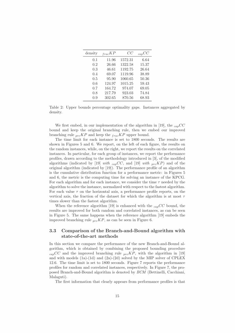
density fracKP CC capCC

0.1 11.96 1572.31 6.640.2 26.66 1322.58 15.370.3 46.61 1192.75 26.640.4 69.07 1119.96 38.890.5 95.90 1060.65 50.360.6 124.97 1015.25 59.430.7 164.72 974.07 69.050.8 217.79 923.03 74.840.9 302.65 870.56 68.93

Table 2: Upper bounds percentage optimality gaps. Instances aggregated bydensity.

We first embed, in our implementation of the algorithm in [19], the capCCbound and keep the original branching rule, then we embed our improvedbranching rule preKP and keep the fracKP upper bound.

The time limit for each instance is set to 1800 seconds. The results areshown in Figures 5 and 6. We report, on the left of each figure, the results onthe random instances, while, on the right, we report the results on the correlatedinstances. In particular, for each group of instances, we report the performanceprofiles, drawn according to the methodology introduced in [3], of the modifiedalgorithms (indicated by [19] with capCC, and [19] with preKP ) and of theoriginal algorithm (indicated by [19]). The performance profile of an algorithmis the cumulative distribution function for a performance metric: in Figures 5and 6, the metric is the computing time for solving an instance of the KPCG.For each algorithm and for each instance, we consider the time τ needed by thealgorithm to solve the instance, normalized with respect to the fastest algorithm.For each value τ on the horizontal axis, a performance profile reports, on thevertical axis, the fraction of the dataset for which the algorithm is at most τtimes slower than the fastest algorithm.

When the reference algorithm [19] is enhanced with the capCC bound, theresults are improved for both random and correlated instances, as can be seenin Figure 5. The same happens when the reference algorithm [19] embeds theimproved branching rule preKP , as can be seen in Figure 6.

3.3 Comparison of the Branch-and-Bound algorithm with

state-of-the-art methods

In this section we compare the performance of the new Branch-and-Bound al-gorithm, which is obtained by combining the proposed bounding procedure

capCC and the improved branching rule preKP , with the algorithm in [19]and with models (1a)-(1d) and (2a)-(2d) solved by the MIP solver of CPLEX12.6. The time limit is set to 1800 seconds. Figure 7 reports the performanceprofiles for random and correlated instances, respectively. In Figure 7, the pro-posed Branch-and-Bound algorithm is denoted by BCM (Bettinelli, Cacchiani,Malaguti).

The first information that clearly appears from performance profiles is that

15

1 2 3 4 5 6 7 8 9 10τ

0.0

0.2

0.4

0.6

0.8

1.0P(r

p,s≤τ

:1≤s≤n

s)

[19] with capCC[19]

(a) Random instances

1 2 3 4 5 6 7 8 9 10τ

0.0

0.2

0.4

0.6

0.8

1.0

P(r

p,s≤τ

:1≤s≤n

s)

[19] with capCC[19]

(b) Correlated instances

Figure 5: Performance profiles for the KPCG algorithm in [19] and the algorithm[19] with capCC, obtained by using the capCC bound. Each curve represents theprobability to have a computing time ratio smaller or equal to τ with respectto the best performing algorithm. On the left we show random instances andon the right correlated ones.

1 2 3 4 5 6 7 8 9 10τ

0.0

0.2

0.4

0.6

0.8

1.0

P(r

p,s≤τ

:1≤s≤n

s)

[19] with preKP

[19]

(a) Random instances

1 2 3 4 5 6 7 8 9 10τ

0.0

0.2

0.4

0.6

0.8

1.0

P(r

p,s≤τ

:1≤s≤n

s)

[19] with preKP

[19]

(b) Correlated instances

Figure 6: Performance profiles for the KPCG algorithm in [19] and the algorithm[19] with preKP , obtained by using the improved branching procedure preKP .Each curve represents the probability to have a computing time ratio smaller orequal to τ with respect to the best performing algorithm. On the left we showrandom instances and on the right correlated ones.

the KPCG is difficult for the CPLEX MIP solver, and that it is worth to designa specialized algorithm, although exploiting the stronger clique model (2a)-(2d)has some advantages on the weaker model (1a)-(1d).

Both Branch-and-Bound algorithms largely outperform the CPLEX MIPsolver; among the two, the newly proposed algorithm improves on the results ofthe reference one [19] on both the computing times and the percentage of solvedinstances. For example, if we consider random instances, the new algorithm isthe fastest for 80% of the instances, and can solve 97.1% of the instances within acomputing time not exceeding 4 times the computing time of the fastest method(τ = 4). The algorithm in [19] is the fastest for 67.9% of the instances, and cansolve 82.2% of the instances within a computing time not exceeding 4 timesthe computing time of the fastest method (τ = 4). If we consider correlated

16

1 2 3 4 5 6 7 8 9 10τ

0.0

0.2

0.4

0.6

0.8

1.0

P(r

p,s≤τ

:1≤s≤n

s)

BCM[19](2a)−(2d)

(1a)−(1d)

(a) Random instances

1 2 3 4 5 6 7 8 9 10τ

0.0

0.2

0.4

0.6

0.8

1.0

P(r

p,s≤τ

:1≤s≤n

s)

BCM[19](2a)−(2d)

(1a)−(1d)

(b) Correlated instances

Figure 7: Performance profiles for the KPCG algorithm in [19], the new Branch-and-Bound algorithm BCM, and the CPLEXMIP solver applied to formulations(2a)-(2d) and (1a)-(1d). Each curve represents the probability to have a com-puting time ratio smaller or equal to τ with respect to the best performingalgorithm.

instances, the new algorithm is the fastest for 77.8% of the instances, and cansolve 92.4% of the instances within 4 times the computing time of the fastestmethod (τ = 4). The algorithm in [19] is the fastest for 41.2% of the instances,and can solve 67.3% of the instances within 4 times the computing time of thefastest method (τ = 4). In addition, we can see that, on the random instances,the proposed Branch-and-Bound algorithm solves 97.3% when τ = 5, whilethe algorithm in [19] reaches at most 89.8% when τ = 10. On the correlatedinstances, the difference between the two algorithms is more evident: BCMsolves 92.9% of the instances when τ = 5 while the algorithm in [19] reaches the75.1% when τ = 10.

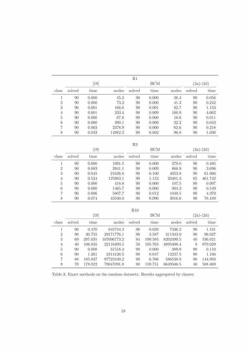
In Tables 3 and 4 we report detailed results for the random and correlatedinstances, respectively, grouped by classes; in Tables 5 and 6 we report detailedresults for random and correlated instances, grouped by density. We omit the re-

17

sults obtained by solving model (1a)-(1d), as they are worse than those obtainedwith model (2a)-(2d). In all tables, the average computing time and number ofnodes are computed with respect to the number of instances optimally solvedby the corresponding method.

Concerning the difficulty of the instances, datasets with tight knapsack con-straints (C1 and R1) are easy for both Branch-and-Bound algorithms and re-quire a smaller number of visited nodes, indeed, all algorithms can solve allinstances. The number of nodes that are explored by BCM, and the corre-sponding computing time, are, on average, significantly reduced with respect tothe Branch-and-Bound in [19], as it can be observed in all the tables, when bothalgorithms solve all instances. In addition, as also shown in the performanceprofiles, BCM solves a larger number instances than both other methods.

Among the 8 classes of instances, class 4 (instances with 1000 items anduniform weights) is the most difficult one, as testified by the number of nodes,the computing times and the number of unsolved instances. In particular fordatasets R10 and C10, which are the most difficult ones, 40 and 50 instancesremain unsolved, respectively, when considering the BCM algorithm, i.e., thebest performing one.

By considering the density of the conflict graphs, we see that instances withvery high densities are easier for the compared Branch-and-Bound algorithms:both algorithms can solve all the instances with densities larger or equal to 0.7,while none can solve all instances with densities between 0.1 and 0.5 in datasetsC10 and R10 i.e., when the knapsack capacity is large.

Low density instances. For the second set of instances, with graph densitiesranging between 0.007 and 0.016, the proposed algorithm is not particularly ef-fective: indeed, it relies on explicitly exploiting incompatibilities between items,and, when the conflict graph is very sparse, other methods, such as [20, 12], aremore efficient.

One may wonder whether methods designed for low density instances couldbe effective on graphs with higher densities. To partially answer this question,we consider the exact method proposed in [12], as it has better performancethan that of [20]. In particular, we focus on the reduction procedure, that is acrucial step of the algorithm proposed in [12]: it consists of fixing some decisionvariables to their optimal values (see [12] for further details). The reductionprocedure is initialized, in [12], with a heuristic solution value obtained by ap-plying the reactive local search algorithm proposed in [11]. Instead, we directlyprovide the reduction procedure with the optimal solution value. It turned outthat, on the first set of instances (with graph densities between 0.1 and 0.9),the reduction procedure is not effective. In particular, on R1 and on C1, eventhough the percentage of fixed variables is high (around 80% on average), thereduction procedures requires long computing times (two order of magnitudelarger than the total time BCM needs to obtain the optimal solutions). On thecontrary, already on R3 and C3, the reduction procedure is not capable of re-ducing the instance size: the percentage of fixed variables is on average around15% and 5%, respectively. Thus, this kind of approach is not appropriate forlarger density graphs.

18

R1[19] BCM (2a)-(2d)

class solved time nodes solved time nodes solved time

1 90 0.000 45.2 90 0.000 26.4 90 0.0562 90 0.000 73.2 90 0.000 41.2 90 0.2423 90 0.001 166.6 90 0.001 82.7 90 1.1534 90 0.001 333.4 90 0.009 160.9 90 4.6625 90 0.000 87.8 90 0.000 16.6 90 0.0116 90 0.000 390.1 90 0.000 32.2 90 0.0437 90 0.003 2378.9 90 0.000 62.6 90 0.2188 90 0.033 14982.2 90 0.002 96.8 90 1.030

R3[19] BCM (2a)-(2d)

class solved time nodes solved time nodes solved time

1 90 0.000 1091.5 90 0.000 279.0 90 0.4952 90 0.003 3941.1 90 0.009 866.9 90 3.6963 90 0.045 21626.8 90 0.100 4053.8 90 61.0664 90 0.524 125983.1 90 1.152 20481.3 65 461.7425 90 0.000 418.8 90 0.000 107.5 90 0.0976 90 0.000 1465.7 90 0.000 304.2 90 0.5497 90 0.006 5807.7 90 0.012 1049.5 90 4.3798 90 0.074 43100.0 90 0.090 3916.6 90 78.189

R10[19] BCM (2a)-(2d)

class solved time nodes solved time nodes solved time

1 90 0.470 845744.2 90 0.028 7336.2 90 1.1012 90 30.755 29171776.1 90 3.587 311343.0 90 96.0273 69 207.035 107696773.2 84 199.585 8202490.5 40 536.0214 40 106.035 22116493.5 50 195.765 4895498.4 8 979.0295 90 0.008 31518.4 90 0.000 389.9 90 0.1106 90 1.261 2314126.5 90 0.047 12237.5 90 1.1667 88 105.037 97723100.2 90 6.766 586538.9 90 144.9938 70 178.822 79047091.8 80 159.751 6649506.5 40 508.469

Table 3: Exact methods on the random datasets. Results aggregated by classes.

19

C1[19] BCM (2a)-(2d)

class solved time nodes solved time nodes solved time

1 90 0.000 495.7 90 0.000 71.4 90 0.1682 90 0.012 8345.8 90 0.001 107.2 90 0.9463 90 0.022 8510.3 90 0.003 177.7 90 5.6304 90 11.828 1913753.8 90 0.010 451.6 90 40.0305 90 0.000 4359.6 90 0.000 164.5 90 0.0216 90 0.016 25241.2 90 0.000 230.1 90 0.0677 90 0.098 65014.7 90 0.001 203.6 90 0.3398 90 0.735 255015.1 90 0.002 338.2 90 2.843

C3[19] BCM (2a)-(2d)

class solved time nodes solved time nodes solved time

1 90 0.005 12930.4 90 0.003 1948.4 90 1.5632 90 0.089 79040.6 90 0.061 11126.6 90 32.5723 90 2.008 1029233.1 90 0.955 80368.4 72 413.5284 88 64.828 17624047.3 90 19.443 761690.3 21 209.6315 90 0.031 109383.5 90 0.000 827.9 90 0.1356 88 69.174 120484341.8 90 0.005 2831.3 90 1.4707 70 8.198 7365262.0 90 0.064 14061.9 90 35.5668 60 34.744 14750601.3 90 0.686 82463.3 79 342.026

C10[19] BCM (2a)-(2d)

class solved time nodes solved time nodes solved time

1 90 24.508 46535034.1 90 0.847 390718.0 90 2.3492 61 21.300 18558165.0 86 149.856 27200583.0 75 212.9053 50 182.781 68685161.7 54 149.385 18954904.4 24 712.5344 30 53.275 12702323.9 40 151.904 10968827.5 0 05 90 0.811 2954067.7 90 0.008 9454.4 90 0.1896 88 76.573 149901735.6 90 2.765 1266635.1 81 2.7187 60 17.971 13926764.8 77 114.528 21362729.7 63 250.6308 50 184.604 68934062.6 50 22.482 2843795.3 20 800.996

Table 4: Exact methods on the correlated datasets. Results aggregated byclasses.

20

R1[19] BCM (2a)-(2d)

density solved time nodes solved time nodes solved time

0.1 80 0.012 6811.3 80 0.001 31.6 80 0.1260.2 80 0.009 4482.8 80 0.000 35.1 80 0.2500.3 80 0.006 2998.1 80 0.001 44.9 80 0.4080.4 80 0.006 2588.0 80 0.001 60.2 80 0.5410.5 80 0.005 1896.8 80 0.001 62.6 80 0.6850.6 80 0.002 950.1 80 0.002 75.1 80 0.7920.7 80 0.001 537.4 80 0.003 86.3 80 1.2060.8 80 0.000 302.5 80 0.002 94.1 80 1.6780.9 80 0.000 197.6 80 0.003 94.4 80 2.656

R3[19] BCM (2a)-(2d)

density solved time nodes solved time nodes solved time

0.1 80 0.026 20333.5 80 0.004 274.1 80 0.1240.2 80 0.028 13781.9 80 0.031 1241.2 80 0.5430.3 80 0.067 21820.6 80 0.132 2923.2 80 5.6300.4 80 0.137 35977.3 80 0.279 5312.3 80 44.3250.5 80 0.180 44764.2 80 0.401 7877.4 77 89.0220.6 80 0.158 42919.7 80 0.387 8415.2 73 97.6610.7 80 0.090 29528.4 80 0.208 5553.8 71 80.6260.8 80 0.037 14777.2 80 0.072 2425.7 74 118.0570.9 80 0.011 4961.3 80 0.018 918.3 80 136.017

R10[19] BCM (2a)-(2d)

density solved time nodes solved time nodes solved time

0.1 69 110.369 88023913.8 70 14.340 652371.4 78 105.3060.2 48 212.425 200328771.6 54 100.734 4412874.2 50 144.0090.3 50 26.802 21984852.8 70 315.999 13251314.6 50 139.5750.4 70 260.592 101365617.8 70 23.951 1125284.5 50 65.7280.5 70 20.220 7493461.6 80 114.559 2904611.6 50 38.7710.6 80 50.684 10770967.7 80 9.434 267046.5 50 25.6600.7 80 3.968 1011439.6 80 1.190 44200.2 70 402.6290.8 80 0.358 111981.9 80 0.191 7977.5 70 167.6140.9 80 0.031 12384.8 80 0.026 1509.0 70 38.564

Table 5: Exact methods on the random datasets. Results aggregated by density.

21

C1[19] BCM (2a)-(2d)

density solved time nodes solved time nodes solved time

0.1 80 12.337 1972293.4 80 0.000 79.0 80 0.1010.2 80 0.880 188977.5 80 0.000 90.6 80 0.2480.3 80 0.272 90194.7 80 0.000 111.0 80 0.4640.4 80 0.147 63056.6 80 0.001 202.6 80 0.6070.5 80 0.302 104502.7 80 0.001 168.3 80 1.0280.6 80 0.246 91745.9 80 0.004 270.1 80 4.0880.7 80 0.083 37551.2 80 0.003 274.5 80 4.8230.8 80 0.027 14043.1 80 0.004 357.4 80 17.4500.9 80 0.006 3463.0 80 0.005 408.6 80 27.491

C3[19] BCM (2a)-(2d)

density solved time nodes solved time nodes solved time

0.1 56 163.731 206171329.1 80 0.051 3667.9 79 8.6400.2 60 3.792 1837069.9 80 0.567 26078.8 80 34.7280.3 70 15.724 9309906.6 80 3.422 120223.8 72 55.2210.4 80 32.466 12229559.4 80 5.568 190780.4 69 90.4090.5 80 11.195 2494963.8 80 8.279 351816.9 66 198.4290.6 80 5.598 1451069.2 80 4.300 252950.2 52 83.9070.7 80 1.950 594962.3 80 1.320 95969.1 64 336.6180.8 80 0.530 168275.2 80 0.305 26311.1 70 135.9910.9 80 0.080 28463.3 80 0.058 6934.7 70 77.380

C10[19] BCM (2a)-(2d)

density solved time nodes solved time nodes solved time

0.1 29 195.022 384555162.0 47 203.917 36828873.3 35 100.3200.2 30 116.997 221125214.2 36 260.334 46619765.3 30 2.9700.3 30 3.204 5552855.4 50 57.207 13484306.0 38 319.9440.4 50 39.479 30808014.2 54 132.369 17104415.3 50 218.6650.5 70 250.275 94082917.5 70 29.312 3776521.3 50 79.2380.6 70 13.200 5351330.9 80 72.695 5359030.3 50 46.1250.7 80 19.800 4900728.8 80 5.405 441719.0 50 26.4220.8 80 1.163 343428.4 80 0.375 32385.0 70 281.3330.9 80 0.078 28554.0 80 0.061 7139.2 70 162.185

Table 6: Exact methods on the correlated datasets. Results aggregated bydensity.

22

4 Conclusion

The Knapsack Problem with Conflict Graph is a relevant extension of the 0-1Knapsack Problem in which incompatibilities between pairs of items are defined.It has received considerable attention in the literature as a stand-alone problem,as well as a subproblem arising in solving, e.g., the Bin Packing Problem withConflicts. The problem is computationally challenging, and cannot be easilytackled through a Mixed-Integer formulation solved with a general purpose MIPsolver.

In this paper a new Branch-and-Bound algorithm, based on improved upperbounding and branching procedures, is proposed. Its performance is tested ona set of instances derived from classical Bin Packing Problems, having graphdensities between 0.1 and 0.9. The obtained results show that the Branch-and-Bound algorithm outperforms, in our implementation, a recent state-of-the-art algorithm from the literature, as well as a Mixed Integer Programmingformulation tackled through a general purpose solver.

References

[1] H. Akeb, M. Hifi, and M. E. Ould Ahmed Mounir. Local branching-basedalgorithms for the disjunctively constrained knapsack problem. Computers& Industrial Engineering, 60(4):811–820, 2011.

[2] R. Carraghan and P. M. Pardalos. An exact algorithm for the maximumclique problem. Operations Research Letters, 9(6):375–382, 1990.

[3] E. D. Dolan and J. J. More. Benchmarking optimization software withperformance profiles. Mathematical Programming, 91:201–213, 2002.

[4] S. Elhedhli, L. Li, M. Gzara, and J. Naoum-Sawaya. A branch-and-pricealgorithm for the bin packing problem with conflicts. INFORMS Journalon Computing, 23(3):404–415, 2011.

[5] E. Falkenauer. A hybrid grouping genetic algorithm for bin packing. Jour-nal of heuristics, 2(1):5–30, 1996.

[6] A.E. Fernandes-Muritiba, M. Iori, E. Malaguti, and P. Toth. Algorithms forthe bin packing problem with conflicts. INFORMS Journal on Computing,22(3):401–415, 2010.

[7] M. Fischetti and A. Lodi. Local branching. Mathematical programming, 98(1-3):23–47, 2003.

[8] M. Gendreau, G. Laporte, and F. Semet. Heuristics and lower bounds forthe bin packing problem with conflicts. Computers & Operations Research,31:347–358, 2004.

[9] S. Held, W. Cook, and E.C. Sewell. Maximum-weight stable sets and safelower bounds for graph coloring. Mathematical Programming Computation,4:363–381, 2012.

23

[10] M. Hifi. An iterative rounding search-based algorithm for the disjunc-tively constrained knapsack problem. Engineering Optimization, 46(8):1109–1122, 2014.

[11] M. Hifi and M. Michrafy. A reactive local search-based algorithm for thedisjunctively constrained knapsack problem. Journal of the OperationalResearch Society, 57(6):718–726, 2006.

[12] M. Hifi and M. Michrafy. Reduction strategies and exact algorithms forthe disjunctively constrained knapsack problem. Computers & operationsresearch, 34(9):2657–2673, 2007.

[13] M. Hifi and N. Otmani. An algorithm for the disjunctively constrainedknapsack problem. International Journal of Operational Research, 13(1):22–43, 2012.

[14] R. M. Karp. Reducibility among combinatorial problems. In R. E. Miller,J. W. Thatcher, and J. D. Bohlinger, editors, Complexity of ComputerComputations, The IBM Research Symposia Series, pages 85–103. SpringerUS, 1972.

[15] H. Kellerer, U. Pferschy, and D. Pisinger. Knapsack problems. Springer,2004.

[16] E. Malaguti, M. Monaci, and P. Toth. An exact approach for the vertexcoloring problem. Discrete Optimization, 8:174–190, 2011.

[17] S. Martello and P. Toth. Knapsack problems. Wiley New York, 1990.

[18] U. Pferschy and J. Schauer. The knapsack problem with conflict graphs.J. Graph Algorithms Appl., 13(2):233–249, 2009.

[19] R. Sadykov and F. Vanderbeck. Bin packing with conflicts: a genericbranch-and-price algorithm. INFORMS Journal on Computing, 25(2):244–255, 2013.

[20] T. Yamada, S. Kataoka, and K. Watanabe. Heuristic and exact algorithmsfor the disjunctively constrained knapsack problem. Information ProcessingSociety of Japan Journal, 43(9), 2002.

24