A Boundary Element Method for EddyCurrents

A Master’s Thesis on the Magnetic Field Method for the Calculation ofEddy Currents on Surfaces with Complicated Geometries

Oded Stein, ETH Zurich

Supervised by:Prof. Dr. Ralf Hiptmair, ETH Zurich

10. April, 2015

ii

Abstract

This master’s thesis explores a method to calculate the magnetic field generated by eddycurrents. It was introduced in a previous work by R. Hiptmair. The method is valid foreddy currents generated by quasi-stationary exciting magnetic fields.

Inside the conductor a normal vectorial Maxwell problem is solved using vectorialboundary element methods. Outside the conductor, for domains with trivial first coho-mology group, a scalar potential approach is used. For more complicated domains thatdo not have trivial first cohomology groups a more intricate special scalar potential withcertain discontinuities is used. This allows to apply scalar boundary element methods onthe outside of the conductor. For this case, new Calderon identities for the scalar prob-lem are introduced. On the boundary of the conductor itself the equations are coupledto solve the full eddy current problem.

The method is tested for various geometries and compared to exact solutions whereavailable.

If the domain outside the conductor does not have a trivial first cohomology groupthe method as constructed is dependent on the construction of cutting surfaces. Thisthesis manages to remove this dependence and reduce computations to the boundary ofthe cutting surfaces only. These boundaries correspond to homology cycles.

iii

Acknowledgements

I would like to thank Prof. Ralf Hiptmair of ETH Zurich for supervising me and helpingme with all my problems during the writing process. Prof. Hiptmair wrote the paperwhich introduced the magnetic field based method and was the basis for this thesis.

I would also like to thank Dr. Lars Kielhorn and Elke Spindler of ETH Zurich whoassisted me with BETL2 and all sorts of technical infrastructure without which all thecalculations of this thesis would not have been possible. I also thank Nicolaus Heuerwho helped me with the idea for the proof in Chapter 9.

I am grateful for the ETH Foundation’s Excellence Scholarship and OpportunityAward which financed my master’s degree studies and made this thesis possible.

Lastly, I would like to thank my family and friends who supported me throughout mystudies at ETH Zurich and during the writing of this thesis (and who helped me withgrammar and spelling).

iv

Contents

1 Introduction 1

2 Eddy current model problem 32.1 Domain . . . . . . . . . . . . . . . . . . . . . . . . . . . . . . . . . . . . . 32.2 Maxwell equations . . . . . . . . . . . . . . . . . . . . . . . . . . . . . . . 42.3 Approximations . . . . . . . . . . . . . . . . . . . . . . . . . . . . . . . . . 52.4 Potentials . . . . . . . . . . . . . . . . . . . . . . . . . . . . . . . . . . . . 62.5 Exciting field . . . . . . . . . . . . . . . . . . . . . . . . . . . . . . . . . . 62.6 Reaction field . . . . . . . . . . . . . . . . . . . . . . . . . . . . . . . . . . 62.7 Continuity along interfaces . . . . . . . . . . . . . . . . . . . . . . . . . . 7

3 Function spaces 83.1 Spaces . . . . . . . . . . . . . . . . . . . . . . . . . . . . . . . . . . . . . . 83.2 Traces . . . . . . . . . . . . . . . . . . . . . . . . . . . . . . . . . . . . . . 9

4 Boundary integral operators 104.1 Operators for scalar-valued functions . . . . . . . . . . . . . . . . . . . . . 104.2 Operators for vector-valued functions . . . . . . . . . . . . . . . . . . . . . 11

5 The method for simple geometries 145.1 Inside the conductor . . . . . . . . . . . . . . . . . . . . . . . . . . . . . . 145.2 Outside the conductor . . . . . . . . . . . . . . . . . . . . . . . . . . . . . 155.3 Combining inside and outside . . . . . . . . . . . . . . . . . . . . . . . . . 16

6 Implementation of the method for simple geometries 186.1 Discretization of spaces and operators in BETL2 . . . . . . . . . . . . . . 186.2 The discretized boundary integral equation . . . . . . . . . . . . . . . . . 206.3 Results . . . . . . . . . . . . . . . . . . . . . . . . . . . . . . . . . . . . . . 20

7 Derivation of the method for complicated geometries 237.1 Inside the conductor . . . . . . . . . . . . . . . . . . . . . . . . . . . . . . 237.2 Outside the conductor . . . . . . . . . . . . . . . . . . . . . . . . . . . . . 237.3 Combining inside and outside . . . . . . . . . . . . . . . . . . . . . . . . . 35

8 Implementation of the method for complicated geometries 398.1 Discretization of the jump spaces . . . . . . . . . . . . . . . . . . . . . . . 398.2 Testing the Calderon identities . . . . . . . . . . . . . . . . . . . . . . . . 41

v

8.3 The eddy current problem . . . . . . . . . . . . . . . . . . . . . . . . . . . 43

9 Removing the cutting surfaces 499.1 Theory . . . . . . . . . . . . . . . . . . . . . . . . . . . . . . . . . . . . . . 499.2 Algorithm . . . . . . . . . . . . . . . . . . . . . . . . . . . . . . . . . . . . 52

10 Conclusion 53

11 Appendix 5411.1 Implementation of finite element spaces . . . . . . . . . . . . . . . . . . . 5411.2 Combinatorial gradient, curl and divergence . . . . . . . . . . . . . . . . 5911.3 Mass matrices . . . . . . . . . . . . . . . . . . . . . . . . . . . . . . . . . 6011.4 Adding constraints to functions . . . . . . . . . . . . . . . . . . . . . . . 6011.5 BEM operators . . . . . . . . . . . . . . . . . . . . . . . . . . . . . . . . . 6111.6 Incorporating boundary conditions and the ansatz function . . . . . . . . 6211.7 Visualization . . . . . . . . . . . . . . . . . . . . . . . . . . . . . . . . . . 63

12 Bibliography 64

vi

1 Introduction

Eddy currents are currents induced in an electric conductor when it is moved througha magnetic field (ref. [11, p.298]). The eddy currents create magnetic fields which in-teract with the magnetic field present and often significantly change the dynamics ofthe system. As [11, p.298] states, “eddy currents are notoriously difficult to calculate.”Nevertheless they are of importance as metals moving in magnetic fields are abundantin engineering applications.

This master’s thesis explores a boundary element method to calculate eddy currentson the surfaces of conductors moving slowly through exciting magnetic fields. Thesemagnetic fields are generated by closed electric currents (such as in a coil or a circularwire). This work deals with the motivation of the model, the derivation of the bound-ary element method, the implementation of the boundary element method and possiblesimplifications of it.

In published literature one can find multiple methods for calculating these eddy cur-rents, such as a boundary element method based on the electric field (mentioned in [13]and [14]) or a mixed BEM-FEM approach as mentioned in [24].In [13] Ralf Hiptmair derives multiple boundary element methods for the calculation ofeddy currents and explores two of them in detail: one is based on formulating the prob-lem with electric fields and the other is based on formulating the problem with magneticfields. The magnetic field method from [13] relies on a scalar potential formulation of themagnetic field outside the conductor. This formulation allows the use of scalar boundaryelement methods outside the conductor but places some requirements on the geometryof the conductor. These geometrical constraints can lead to a complicated formulation.This thesis builds on [13] and explores the method based on magnetic fields formulatedthere. An attempt is made to simplify some of the complications stemming from thegeometry of the problem. [13] has an error in formulating the Calderon identities for thecase of objects with complicated geometries. This error is fixed in this thesis.

In Chapter 2 the eddy current model is introduced. This model is a simplificationof the Maxwell equations under specific assumptions which are discussed there. Thechapter also introduces standard notation for the electric and magnetic fields and theirrespective potentials.

Chapter 3 deals with the functional analysis framework in which the calculations ofthis thesis happen. It introduces the proper definition and setup of the function spacesand the traces for the boundary. Function spaces and trace spaces for the magnetic fieldsand the potentials are introduced and justified.

1

The basic theory for the boundary element method is introduced in Chapter 4. Itconsists of standard theory developed elsewhere that forms the basis for most boundaryelement methods. Also, a standard notation for all operators is introduced.

Chapter 5 then deals with the application of boundary element theory to constructboundary integral equations for the case where the conductor has a simple geometry.The method consists of coupling boundary integral equations on the inside and on theoutside of the conductor. Simple geometry means that the complement of the conductorhas trivial first cohomology group.

In Chapter 6 the boundary integral equations from Chapter 5 are discretized and amatrix equation is formulated to solve the problem computationally. An implementationis provided using the framework of BETL2 [20] for the case where the conductor is asphere.

As the theory from Chapter 5 only holds for simple geometries, Chapter 7 introducesboundary integral equations that allow conductors with more general geometries. Thecorresponding boundary integral equations are derived; they differ substantially fromthe rather standard equations in Chapter 5.

Chapter 8 deals with the discretization and implementation of the equations derived inChapter 5. First the new boundary integral equations are tested by themselves, then thecoupled eddy current problem itself is solved. A few issues remain, these are discussed.

The formulation in Chapter 7 and Chapter 8 includes cutting surfaces. These arespecial surfaces that are needed for the method, however the method is to some degreeindependent of the specific choice of cutting surfaces. In fact, the method can be reducedto just the boundary of these cutting surfaces. This is discussed in Chapter 9.

Finally, Chapter 10 summarizes the thesis and gives an outlook on possible futurework.

The appendix (Chapter 11) contains code snippets that show how the methods appliedthroughout the thesis are actually implemented using the BETL2 framework [20]. Thesnippets are referenced throughout the thesis but moved to the appendix for readabilitypurposes.

2

2 Eddy current model problem

As stated in the introduction, eddy currents are caused by time-varying magnetic fieldsin conductors. In this model the magnetic field will be caused by an exciting current js.The conductor Ωc, the interior of its complement Ωe and the boundary between themform the domain.

2.1 Domain

The domain consists of the conductor, a bounded open Ωc in R3, the interior of thecomplement of the conductor, Ωe, which is empty space and the boundary between theconductor and the air which is called Γ. A sketch of the situation for a model problem(the simple geometry, which will be discussed in Chapters 5 and 6) can be seen in Figure2.1.It is assumed that the conductor is simple, linear, homogeneous and isotropic withconstant conductivity σ > 0 and constant permeability µc > 0 (these approximationsare from the model used in [13] which introduces them in Section 2). It is also assumedthat the exciting current js is compactly supported outside the conductor.Additionally it is assumed that the surface of Ωc, Γ, is a smooth closed manifold. Inpractice it will consist of piecewise polygons (which may be curved), as the input for thenumerical method will be a mesh of triangles.

3

Figure 2.1: Sketch of the domain; the conductor Ωc in gray and the exciting current jsin red

2.2 Maxwell equations

The eddy current model is based on the Maxwell equations. The basic Maxwell equations(this version is taken from [11, p.330]) are:

div D = ρf

div B = 0

curl E = −∂B

∂t

curl H = jf +∂D

∂t

(2.1)

H is understood to be 1µB (because of the linear material, ref. [11, p.382]). D is

understood to be εE. ρf and jf are free charge and free current respectively. Theconductivity of the material is denoted by σ.From now on free charge will be assumed to be 0.

This version of the Maxwell equations is just one version; there are other versions thatmay differ by scaling (ref. [11, p.326]). However, all describe the same physics.

In frequency domain (after a Fourier transform), the Maxwell equations are:

4

div D = 0

div B = 0

curl E = −iωB = −iωµH

curl H = jf + iωD

(2.2)

where ω is the frequency.

2.3 Approximations

Some simplifications are made to the Maxwell equations in the eddy current model. It isassumed that the field is quasi-stationary without displacement current (this is justifiedin e.g. [7, p.151], [13, Chapter 2]).This is a good approximation if ωε0 σ (where ε0 is the permittivity of vacuum). As[13, Chapter 1] states, this means that the timescale is long enough so that space chargesdo not need to be taken into account (this is the quasi-stationary part). This generallyholds “for good conductors and frequencies which are not too high” [7, p.151].It is also necessary that the field is slowly varying, or as [7, (30)] puts it, ωL

c 1 withc the speed of light and L the maximum distance that can occur between two points inthe conductor (this is the same requirement as [13, (1)]).

Omitting the displacement current turns (2.2) into:

div D = 0

div B = 0

curl E = −iωµH

curl H = jf

(2.3)

Outside the conductor the free current is just the exciting current js. Inside the con-ductor (where there is conductivity) Ohm’s law gives jf = σE (ref. [11, p.285]). Ohm’slaw is a simplification of the Lorentz force law if the velocity of the charges is so smallthat it can be disregarded (which is assumed here).

The final equations governing the model are thus:

div E = 0

div B = 0

curl E = −iωµH

curl H =

js in Ωe

σE in Ωc

(2.4)

This corresponds to the model used in [13, p.216].

5

2.4 Potentials

As usual in electromagnetics it is possible to define potentials for the electric and mag-netic fields. These are introduced here so that they can be used later on.Similar to [11, pp.416] the way to define the magnetic potential A is such that B =curl A. The gauge is chosen such that div A = 0.Again similar to [11, pp.416] the way to define the electric potential V is such thatE = −gradV − iωA. As there are no free charges it is possible to set V = 0. This givesE = −iωA and is called temporal gauge (ref. e.g. [18, p.676]).

This is consistent with the potentials as defined in [13, p.217].

2.5 Exciting field

The exciting current can be any sufficiently regular current as long as div js = 0 (whichmeans the current is closed). The exciting current creates the two exciting fields Es andHs. By Maxwell clearly div Hs = 0 and as there are no free electric charges div Es = 0.(2.3) together with the definition of the magnetic field then gives:

curl Es = −iωµ0Hs

curl Hs = js(2.5)

It is possible to conclude that:

Hs = − 1

iωµ0curl Es (2.6)

This is consistent with [13, p.217].

2.6 Reaction field

In Ωe it makes sense to introduce the so-called reaction fields (ref. [13, p.217]) Er :=E−Es and Hr := H−Hs. (2.5) then gives:

curl Hr = 0 in Ωe

curl curl Er = 0 in Ωe(2.7)

Thus outside the conductor (Ωe) there is a double pair of fields: the exciting fields Hs

and Es and the reaction fields Hr and Er. Inside the conductor (Ωc) the fields H andE will be called total fields, following the naming convention of [13].

6

2.7 Continuity along interfaces

There are multiple areas with different conductivity and permittivity in this model. Be-cause of this, jumps of the fields along interfaces occur. Jumps across the surface Γ arewritten as [·]Γ.

For the magnetic field, [11, pp.273] states (where ⊥ denotes the perpendicular part ofthe field and || denotes the parallel part of the field):

[B⊥]Γ = 0 ⇒ µ0H⊥s + µ0H

⊥r = µcH

⊥

H||s + H||r = H|| + Kf × n = H||(2.8)

(Kf , the free surface current, is 0)

For the electric field, [11, pp.178] states:

E⊥s + E⊥r = E⊥

1

µ0E||s +

1

µ0E||r =

1

µcE||

(2.9)

These jump conditions can also be formulated using the trace operators from Chapter3. They will be repeated in that chapter with updated notation.

7

3 Function spaces

In this chapter the various function spaces needed for the correct formulation of boundaryintegral equations are introduced, as well as the traces associated with them. The spacesare formulated similarly to [13].

3.1 Spaces

Definition 3.1 The space for the magnetic field is (ref. [13, p.218]):

H(curl; Ω) := Φ ∈ L2(Ω); curl Φ ∈ L2(Ω) (3.1)

This can be justified physically. As e.g. [11, p.319] states the magnetic energy is anintegral of the vector potential and the current, A · j (times a constant). As the currentis the curl of the magnetic field (times a constant), the field and its curl should be inL2(Ω) in order to ensure that the energy is finite.One needs to be more diligent with formulating a space for the electric field, but as thisthesis only discusses methods based on the magnetic field it can be ignored for now.

Additionally, certain scalar traces formulated in the following section will need thestandard Sobolev-Hilbert spaces:

H1(Ω) := ϕ ∈ L2(Ω); Dϕ ∈ L2(Ω) (3.2)

and the associated H0(Ω), H12 (Ω), H−

12 (Ω). Theory for these can be found in standard

PDE texts such as [9].It is also necessary to introduce the following space (ref. e.g. [13, p.219]):

H1(4,Ω) := ϕ ∈ H1(Ω); 4ϕ ∈ L2(Ω) (3.3)

Definition 3.2 The different traces will map into different function spaces on the bound-ary. These are:

H− 1

2⊥ (curlΓ,Γ) := Φ ∈H

− 12⊥ (Γ); curlΓΦ ∈H−

12 (Γ)

H− 1

2

|| (divΓ,Γ) := Φ ∈H− 1

2

|| (Γ); divΓΦ ∈ H−12 (Γ)

(3.4)

which are based on the Sobolev-Hilbert spaces H− 1

2

|| (Γ) (functions with tangential con-

tinuity) and H− 1

2⊥ (Γ) (functions with normal continuity) on the boundary (ref. [13,

pp.218]). According to e.g. [13, p.219] or [4, Part II] the second space is the dual ofthe first with respect to the usual L2(Ω) duality pairing.

8

3.2 Traces

Definition 3.3 The following trace is the Dirichlet-like trace for the space H(curl; Ω):

γt : H(curl; Ω)→H− 1

2⊥ (curlΓ,Γ) γtΦ := n× (Φ× n)

∣∣Γ

(3.5)

The definition on the right only holds for smooth functions, but is easily extended toall Sobolev functions in the respective space. This trace is called Dirichlet or tangentialtrace.

The vector n is understood as the outward normal vector of Ωc. The definition coincideswith the one from [13, p.219].

Definition 3.4 The following two traces are Neumann-like traces for the vectorial spaces:

γN : H(curl curl,Ω)→H− 1

2

|| (divΓ,Γ) γNΦ := curl Φ× n∣∣Γ

γn : H(div; Ω)→ H−12 (Γ) γnΦ := n ·Φ

∣∣Γ

(3.6)

The definitions on the right again hold for smooth functions, but are easily extended toall Sobolev functions in the respective space. They will be called Neumann and normaltrace.

For the Neumann trace, [13] uses a Beppo-Levi-type space. As this thesis will not dealwith the electric fields that live in this space, the normal curl space will suffice. Thedefinitions coincide with [13, p.220].

For non-vectorial functions there are the standard Dirichlet and Neumann traces (asfor example used in [26]). They will be denoted by:

γ : H1(Ω)→ H12 (Γ)

∂n : H1(4,Ω)→ H−12 (Γ)

(3.7)

According to [13, Chapter 3] these are the correct trace spaces.

With the notation for trace operators the jump conditions for the magnetic field for-mulated in (2.8) are:

µ0γenHs + µ0γ

enHr = µcγ

cnH

γetHs + γetHr = γctH(3.8)

where the superscript e denotes that the trace is taken from the outside and the super-script c denotes that the trace is taken from the inside of the conductor.

9

4 Boundary integral operators

In this chapter the boundary integral operators and their Calderon identities are intro-duced. These operators are later used to formulate boundary integral equations andsolve the eddy current problem.On the outside of the conductor, where there is 0 conductivity, the problem will be solvedlike a scalar potential problem. The theory for this is well-established and will be basedon [28] in this thesis with notation from [13] for compatibility.On the inside of the conductor the situation is more complicated. A vector-valuedcurl curl problem has to be solved. Theory for this will be taken from [5], with notationfrom [13].

4.1 Operators for scalar-valued functions

[28, p.111] gives the following fundamental solution to the Laplace equation in 3D:

G0(x, y) :=1

4π

1

|x− y| (4.1)

With this fundamental solution the boundary integral operators can be defined:

Definition 4.1 The Laplace single layer operator V 0, the double and adjoint doublelayer operators K0, K0,∗ and the hypersingular operator D0 are defined (ref. e.g. [28,pp.118], [13, p.225]) as following:

V 0 := γcΨ0V : H−

12 (Γ)→ H

12 (Γ),

(Ψ0V ϕ)(x) :=

∫ΓG0(x, y)ϕ(y)dS(y), x /∈ Γ

K0,∗ :=1

2(∂cn + ∂en)Ψ0

V : H−12 (Γ)→ H−

12 (Γ)

K0 :=1

2(γc + γe)Ψ0

K : H12 (Γ)→ H

12 (Γ),

(Ψ0Kϕ)(x) :=

∫Γ(∂cnyG0(x, y))ϕ(y)dS(y), x /∈ Γ

D0 := −∂cnΨ0K

(4.2)

where the superscript c means approaching from inside the conductor and the superscripte approaching from outside the conductor. Ψ0

V and Ψ0K are called single and double layer

potential respectively.

10

The adjoint double layer operator can easily be expressed using the double layer oper-ator as one is the adjoint of the other in the duality pairing of H−

12 (Γ) and H

12 (Γ) (ref.

[28, p.152]).[28, Theorem 6.17] gives a more convenient representation for the hypersingular operatoron closed surfaces with continuous functions:

〈Du, v〉Γ =1

4π

∫Γ

∫Γ

curlΓu(y) · curlΓv(x)

|x− y|dS(x)dS(y) (4.3)

where 〈·, ·〉 is the L2 scalar product.

For Ψ0V and Ψ0

K , the following jump relations hold as of [28, pp.118]:

[γΨ0V ]Γ = 0 [∂nΨ0

V ]Γ = − id

[γΨ0K ]Γ = id [∂nΨ0

K ]Γ = 0(4.4)

These operators together with the jump relations and the representation formula [28,(6.1)] give the internal and external Calderon identity for the Laplace equation:

Lemma 4.2 For u ∈ H1(Γ) solving the Laplace equation −4u = 0 on Ωc ∪Ωe it holds:(γcu∂cnu

)=

(12 id−K0 V 0

D0 12 id +K0,∗

)(γcu∂cnu

)(4.5)

(γeu∂enu

)=

(12 id +K0 −V 0

−D0 12 id−K0,∗

)(γeu∂enu

)(4.6)

Proof Ref. [28, p.137] and [28, p.182].

4.2 Operators for vector-valued functions

For the vectorial case, a representation formula is needed from which a vectorial Calderonidentity is constructed. This formula is taken from [5, Chapter 4].[5] works with the fundamental Helmholtz solution Ek(x, y) = 1

4π|x−y|eik|x−y| to solve a

curl curl−k2 type equation. As this thesis is concerned with solving a curl curl +κ2

type equation, the fundamental solution is (from [13, p.226] for compatibility):

Gκ(x, y) :=1

4π

e−κ|x−y|

|x− y|(4.7)

with κ = −ik, thus κ2 = −k2 and, as in [5] Im(k) > 0 is required, Im(−κ/i) = Im(iκ) =Re(κ) > 0.

11

The vectorial single layer potential is defined as in [5, p.15]:

(ΨκV Φ)(x) :=

∫ΓGκ(x, y)Φ(y)dS(y) (4.8)

The Maxwell single and double layer potentials are defined as in [5, p.15] (for κ 6= 0only):1

ΨκAΦ := Ψκ

V (Φ)− 1

κ2grad Ψκ

V (divΓΦ)

ΨκCΦ := curl Ψκ

V (RΦ)(4.9)

ΨκV is the scalar single layer potential with Helmholtz instead of Laplace fundamental

solution. R denotes the rotation around the outward normal vector by π2 . It is needed

in the formulation because [5] uses a rotated tangential trace instead of the normal tan-gential trace (ref. [13, p.228]).

For ΨκA and Ψκ

C , the following jump relations hold as of [5, Theorem 7]:

[γtΨκA]Γ = 0 [γNΨκ

A]Γ = − id

[γtΨκC ]Γ = − id [γNΨκ

C ]Γ = 0(4.10)

With these operators the Stratton-Chu representation formula [5, p.16] holds:

U = ΨκCγ

ctU + Ψκ

AγcNU (4.11)

for a U such that curl curl U + κ2U = 0.Taking the Dirichlet trace from inside yields (ref. [13, (36)] and [5, Chapter 5]):

γctU = γctΨκCγ

ctU + γctΨ

κAγ

cNU =

(1

2id +Cκ

)γctU + AκγcNU (4.12)

Taking the Neumann trace from inside yields (ref. [13, (36)] and [5, Chapter 5]):

γcNU = γcNΨκCγ

ctU + γcNΨκ

AγcNU = NκγctU +

(1

2id +Bκ

)γcNU (4.13)

where the following definitions were used:

Definition 4.3 The Maxwell single layer operator Aκ, the double and adjoint doublelayer operators Cκ, Bκ and the hypersingular operator Nκ are defined as following (ref.[13, p.229]):

1Note that this is slightly different from the ΨκSL used in [5], as the Neumann trace there is the normal

Neumann trace divided by iκ.

12

Aκ = γctΨκA : H

− 12

|| (divΓ,Γ)→H− 1

2⊥ (curlΓ,Γ)

Cκ =1

2(γct + γet)Ψκ

C : H− 1

2⊥ (curlΓ,Γ)→H

− 12⊥ (curlΓ,Γ)

Bκ =1

2(γcN + γeN )Ψκ

A : H− 1

2⊥ (curlΓ,Γ)→H

− 12⊥ (curlΓ,Γ)

Nκ = γcNΨκC : H

− 12⊥ (curlΓ,Γ)→H

− 12

|| (divΓ,Γ)

(4.14)

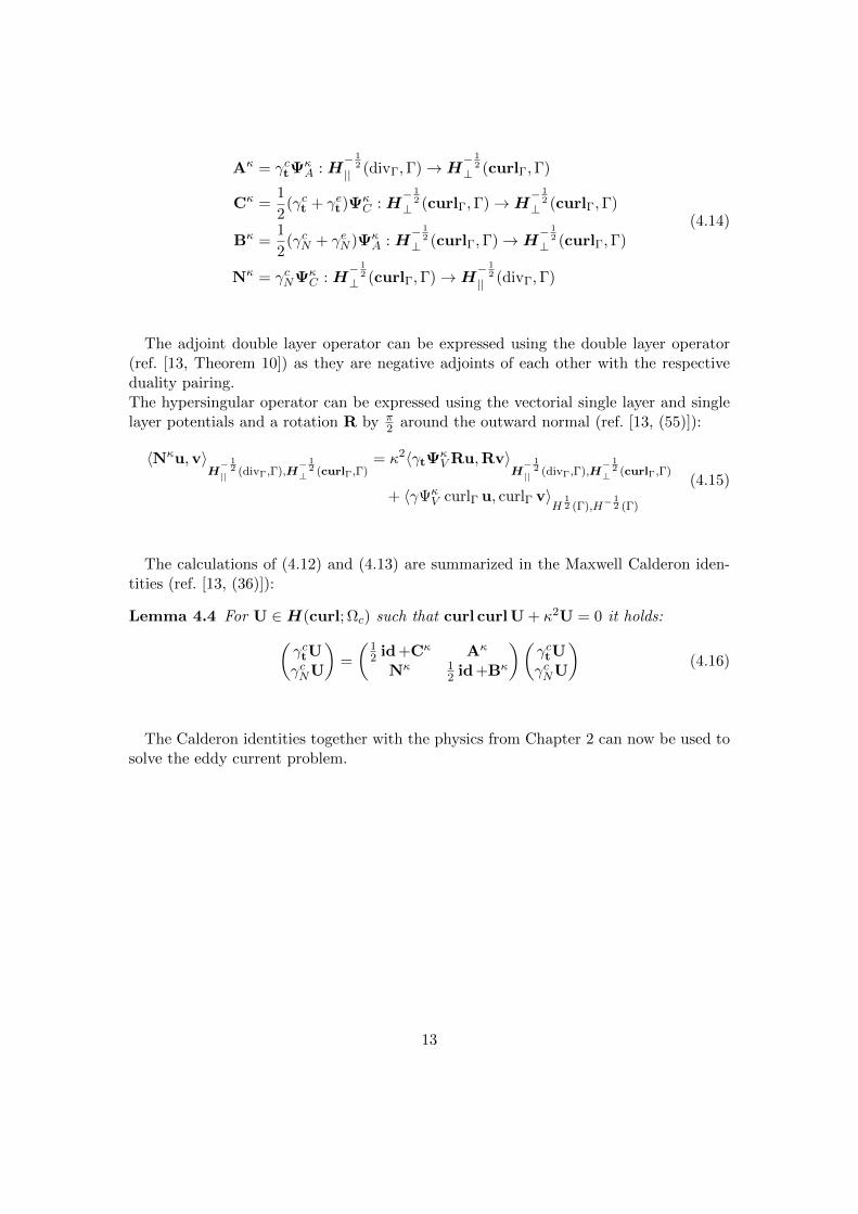
The adjoint double layer operator can be expressed using the double layer operator(ref. [13, Theorem 10]) as they are negative adjoints of each other with the respectiveduality pairing.The hypersingular operator can be expressed using the vectorial single layer and singlelayer potentials and a rotation R by π

2 around the outward normal (ref. [13, (55)]):

〈Nκu,v〉H− 1

2|| (divΓ,Γ),H

− 12⊥ (curlΓ,Γ)

= κ2〈γtΨκV Ru,Rv〉

H− 1

2|| (divΓ,Γ),H

− 12⊥ (curlΓ,Γ)

+ 〈γΨκV curlΓ u, curlΓ v〉

H12 (Γ),H−

12 (Γ)

(4.15)

The calculations of (4.12) and (4.13) are summarized in the Maxwell Calderon iden-tities (ref. [13, (36)]):

Lemma 4.4 For U ∈H(curl; Ωc) such that curl curl U + κ2U = 0 it holds:(γctUγcNU

)=

(12 id +Cκ Aκ

Nκ 12 id +Bκ

)(γctUγcNU

)(4.16)

The Calderon identities together with the physics from Chapter 2 can now be used tosolve the eddy current problem.

13

5 The method for simple geometries

The Calderon identities from Chapter 4 for the Laplace equation (outside) and theMaxwell equation (inside) can now be combined to form a boundary element method tosolve the eddy current problem.

For this chapter it will be assumed that the geometry of Γ is simple, that means Ωe

has trivial first cohomology group. This will allow easy construction of scalar potentialsin the outside region Ωe.

5.1 Inside the conductor

Inside Ωc, (2.4) states:

curl E = −iωµcHcurl H = σE

(5.1)

This gives:

curl curl H = σ curl E = −iωσµcHcurl curl H + κ2H = 0

(5.2)

with κ =√iωσµc. As the physical constants ω, σ, µc are all positive, Reκ > 0.

This allows the application of the Calderon identity (4.16) to the interior total fieldH to obtain: (

γctHγcNH

)=

(12 id +Cκ Aκ

Nκ 12 id +Bκ

)(γctHγcNH

)(5.3)

By (5.2), H = − 1κ2 curl curl H. Testing this with some Φ ∈ H(curl; Ω) gives (with

〈·, ·〉l the duality pairing between the div and curl spaces on the boundary):

〈H,Φ〉L2(Ωc) = − 1

κ2〈curl curl H,Φ〉L2(Ωc)

= − 1

κ2

(〈n× curl H,Φ〉l + 〈curl H, curl Φ〉L2(Ωc)

)= − 1

κ2

(〈γcNH, γctΦ〉l + 〈curl H, curl Φ〉L2(Ωc)

) (5.4)

by integration by parts (integration by parts for curl follows from Gauss’s divergencetheorem as seen in [22, Chapter 12] and basic vector calculus identities as seen in [11,Back matter]).

14

5.2 Outside the conductor

In Ωe, (2.4), (2.7) and the fact that div js = 0 give:

div Hr = 0

curl Hr = 0(5.5)

Now the assumption of trivial first cohomology group will be used:

Lemma 5.1 Let U ∈ H(curl;M) where M is a smooth manifold with trivial firstcohomology group. Then there is a potential function u ∈ H1(4,M) such that gradu =U as long as curl U = 0.The potential is not unique (ref. [13, Chapter 4]).

Proof If the first de Rham cohomology group of M is trivial, for every differential 1-form ω that is a cocycle (i.e. dω = 0) there is a function (a 0-form) u such that du = ω.1

The de Rham theorem (ref. [3, p.287]) states that de Rham and singular cohomologyare isomorphic for smooth manifolds. This means the assumption of trivial first coho-mology group suffices to have this property.

The curl in a differential geometric setting is associated with the exterior derivativeof the corresponding covector 1-form (ref. [3, p.269]), so if ω is the covector field corre-sponding to U, it is a cocycle. The gradient in a differential geometric setting gives thevector field corresponding to the covector 1-form generated by the exterior derivative [3,p.80]. This means gradu = U.

The potential is clearly not unique as any constant function can be added to it withoutchanging its important properties.

This carries over into the non-smooth setting.This means it is possible to introduce a potential function hr such that:

gradhr = Hr

4hr = div Hr = 0(5.6)

This is the Laplace equation. This means the Calderon identity (4.6) applies:(γehr∂enhr

)=

(12 id +K0 −V 0

−D0 12 id−K0,∗

)(γehr∂enhr

)(5.7)

1Terminology in this section is from [3] but should be standard.

15

By the discussion in Chapter 3 and Lemma 5.1, hr should be in H1(4,Ωe). It ispossible to test this with the Dirichlet trace of some ϕ ∈ H1(Ωe) and apply integrationby parts to obtain:

〈gradhr,gradϕ〉L2(Ωe) = 〈n · gradhr, ϕ〉d − 〈4hr, ϕ〉L2(Ωc)

= 〈∂enhr, γeϕ〉d(5.8)

where 〈·, ·〉d denotes the duality pairing between the respective −12 and +1

2 Sobolev-Hilbert spaces on the boundary.

5.3 Combining inside and outside

At this point a decay condition is added that assumes that the magnetic field decayswhen going to infinity fast enough. This makes sense, as H should have finite energy.The two test functions Φ in Ωc and ϕ in Ωe can be combined into a test function for allof R3, V ∈H(curl;R3), curl V

∣∣Ωe

= 0 by piecewise definition:

V := Φ in Ωc

V := gradϕ in Ωe

γctΦ = γet gradϕ

(5.9)

where the usual jump relations (2.8) must hold, but this time with no excitation field.With the decay conditions, (2.4) and more integration by parts (ref. [13, (19)]):2

−iωµ〈H,V〉L2(R3) = 〈curl E,V〉L2(R3) = 〈E, curl V〉L2(R3)

= 〈E, curl Φ〉L2(Ωc) =1

σ〈curl H, curl Φ〉L2(Ωc)

(5.10)

To simplify notation, let µr = µc/µ0 and τ = 1iωµ0σ

= µrκ2 . Split into contributions of

Ωc and Ωe this gives:

−µr〈H,Φ〉L2(Ωc) − 〈gradhr + Hs,gradϕ〉L2(Ωe) = τ〈curl H, curl Φ〉L2(Ωc)

−µr〈H,Φ〉L2(Ωc) − 〈gradhr,gradϕ〉L2(Ωe) − 〈γenHs, ϕ〉d = τ〈curl H, curl Φ〉L2(Ωc)

(5.11)

where in the last step integration by parts and div Hs = 0 are used.

Inserting (5.4) and (5.8) into above equation gives (ref. [13, (51)]):

τ〈γcNH, γctΦ〉l − 〈∂enhr, γeϕ〉d = 〈γenHs, γeϕ〉d (5.12)

2this derivation is also inspired by [2, Chapter 8]

16

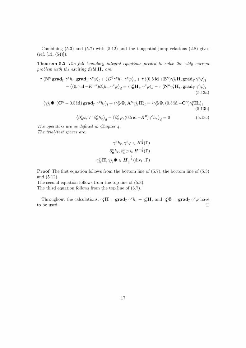
Combining (5.3) and (5.7) with (5.12) and the tangential jump relations (2.8) gives(ref. [13, (54)]):

Theorem 5.2 The full boundary integral equations needed to solve the eddy currentproblem with the exciting field Hs are:

τ 〈Nκ gradΓ γehr,gradΓ γ

eϕ〉l +⟨D0γehr, γ

eϕ⟩d

+ τ 〈(0.5 id +Bκ)γcNH,gradΓ γeϕ〉l

−⟨(0.5 id−K0,∗)∂enhr, γ

eϕ⟩d

= 〈γenHs, γeϕ〉d − τ 〈N

κγetHs,gradΓ γeϕ〉l

(5.13a)

〈γcNΦ, (Cκ − 0.5 id) gradΓ γehr〉l + 〈γcNΦ,AκγcNH〉l = 〈γcNΦ, (0.5 id−Cκ)γetHs〉l

(5.13b)⟨∂enϕ, V

0∂enhr⟩d

+⟨∂enϕ, (0.5 id−K0)γehr

⟩d

= 0 (5.13c)

The operators are as defined in Chapter 4.The trial/test spaces are:

γehr, γeϕ ∈ H

12 (Γ)

∂enhr, ∂enϕ ∈ H−

12 (Γ)

γcNH, γcNΦ ∈H− 1

2

|| (divΓ,Γ)

Proof The first equation follows from the bottom line of (5.7), the bottom line of (5.3)and (5.12).The second equation follows from the top line of (5.3).The third equation follows from the top line of (5.7).

Throughout the calculations, γctH = gradΓ γehr + γetHs and γctΦ = gradΓ γ

eϕ haveto be used.

17

6 Implementation of the method for simplegeometries

This chapter is about the implementation of the boundary element method for simplegeometries (i.e. the ones where the first cohomology group of Ωe is trivial). First the dis-cretization of the functional spaces is discussed, then the discretization of the boundaryelement operators and the boundary element equations. Subsequently the results are pre-sented for the case where Γ is the 2-sphere and are compared with an analytical solution.

The framework used for the implementation that does all the discretization and setupof operators is BETL2 [20]. The actual construction of meshes is done with Gmsh [10]and the visualization is done with Paraview [21].

6.1 Discretization of spaces and operators in BETL2

BETL2 offers tools for the discretization of the boundary functional spaces with functionsof order i with usually i = 0, 1, 2. The following is how the discretized BETL2-spaceswill be called in this thesis:

Definition 6.1 H(0) is the discretization of H−12 (Γ) with piecewise continuous func-

tions of order 0. It has dimension n0.H(1) is the discretization of H

12 (Γ) with continuous piecewise linear functions of order

1. It has dimension n1.

H(div) is the discretization of H− 1

2

|| (divΓ,Γ) with edge functions of order 1. It has di-mension nedge.

H(curl) is the discretization of H− 1

2⊥ (curlΓ,Γ) with edge functions of order 1. It has

dimension nedge.

These are all finite-dimensional vector spaces and the functions mapping between themare always understood as matrices. The way the spaces are actually implemented inBETL2 (using code) can be seen in the appendix in Section 11.1.

For all these spaces, BETL2 has the corresponding single and double layer operatorson a trial space tested with a test space. These will be denoted by ΛκSL(test, trial) andΛκDL(test, trial). The actual implementation of the operators in C++ code is discussedin the appendix in Section 11.5.

18

For gradΓ, curlΓ and divΓ, BETL2 offers the following discretizations respectively:

Gg : H(1)→ H(curl), Gg ∈ Cnedge×n1

Gc : H(1)→ H(div), Gc ∈ Cnedge×n1

Gd : H(div)→ H(0), Gd ∈ Cn0×nedge

(6.1)

These are matrices, their sizes correspond to the respective degrees of freedom of theelement spaces’ discretizations (where Cn×m is the space of complex n ×m matrices).The implementation of these operators in C++ code is discussed in the appendix inSection 11.2.

For purely notational purposes the rotation operator, which rotates around the out-ward unit normal by π

2 is introduced as R. In the implementation with BETL2 this isnot actually needed, as BETL2 rotates automatically depending on which test and trialspaces are used so that the space H(curl) is always matched with its dual H(div).1

The scalar boundary integral operators from Chapter 4 are implemented as follows:

V 0 = Λ0SL(H(0), H(0)), V 0 ∈ Cn0×n0

K0 = Λ0DL(H(0), H(1)), K0 ∈ Cn0×n1

K0,∗ = (K0)T K0,∗ ∈ Cn1×n0

D0 = GTc Λ0SL(H(div), H(div))Gc, D0 ∈ Cn1×n1

(6.2)

As before, these are matrices, their sizes correspond to the respective degrees of freedomof the element spaces’ discretizations. The superscript T denotes the transpose of ma-trices.

The vectorial boundary integral operators are implemented as follows:

Aκ = ΛκSL(H(div), H(div)) +1

κ2GTd ΛκSL(H(0), H(0))Gd

Cκ = ΛκDL(H(div), H(curl))

Bκ = −(Cκ)T

Nκ = κ2RTΛκSL(H(div), H(div))R

Aκ, Cκ, Bκ, Nκ ∈ Cnedge×nedge

(6.3)

As before, these are matrices, their sizes correspond to the respective degrees of freedomof the element spaces’ discretizations. The implementation of Nκ lacks the curlΓ partsfrom (4.15). This is irrelevant however: wherever Nκ will be used in the actual methodit will always be composed with at least one Gg and curlΓ gradΓ = 0.

1In Section 11.2 it is mentioned that the gradient into the curl space is currently implemented incorrectly.This holds for the rotation as well: it happens in the wrong direction. This has to be fixed in codeby simply adding a minus sign.

19

6.2 The discretized boundary integral equation

With all the discretized boundary integral operators defined as matrices, the discretizedversion of Theorem 5.2 is: Seek u ∈ H(1), η ∈ H(div) and ψ ∈ H(0) such that, forδ ∈ H(curl) and ν ∈ H(0):τGTg NκGg + D0 τGTg (0.5M + Bκ) K0,∗ − 0.5M

(Cκ − 0.5M)Gg Aκ 0

0.5M − K0 0 V 0

uηψ

=

Mν − τGTg Nκδ

(0.5M − Cκ)δ0

(6.4)

where M is the respective mass matrix here with the appropriate test and trial space.The implementation of the mass matrices in C++ code is discussed in the appendix inSection 11.3.In the notation of Chapter 5, u corresponds to γehr, η corresponds to γcNH and ψ cor-responds to ∂enhr. The exciting field data δ corresponds to γetHs, the exciting field dataν corresponds to γenHs. The C++ code used for the incorporation of the boundaryconditions is explained in the appendix in Section 11.6.

Using properties of the particular operator allows the simplification of the system to:N −CT −KT

C τAκ 0

K 0 V 0

uηψ

=

fg0

(6.5)

where some notations have been simplified:

N := τGTg NκGg + D0

C := τ(Cκ − 0.5M)Gg

K := 0.5M − K0

f = Mν − τGTg Nκδ

g = τ(0.5M − Cκ)δ

(6.6)

Because of the gauging freedom of scalar potentials there is no unique solution u tothis system. For this to happen the additional constraint that γehr integrates to 0 over Γhas to be incorporated. The way this is done is discussed in the appendix in Section 11.4.

6.3 Results

The equation (6.5) has been solved for a sphere with radius a = 0.05 sitting inside asimple wire coil of radius b = 0.065 on which a constant current j0 = 106 is the exciting

20

number of bdryelements rel. error u rel. error η rel. error ψ

128 0.335 0.232 0.234

512 0.163 0.111 0.0785

2048 0.080 0.052 0.022

8192 0.040 0.025 0.007

Table 6.1: L2 errors of the method described in this chapter. u is compared to the exactsolution, ψ is compared to an interpolation of the exact solution in H(0) andη is not compared to the exact Neumann trace of the interior magnetic field,but to minus its conjugate.

current. The calculation of the corresponding magnetic field given this current can befound in [17, pp.181]. The analytical solution to compare with is taken from [25].Further parameters are ω = 2π · 104, σ = 2 · 106, µr = 10. The linear system was solvedwith Eigen’s partialPivLu [8].

A picture of the method’s results can be seen in Figure 6.1, a table with error analysiscan be seen in Table 6.1. The C++ code that is used to produce the visualization isexplained in the appendix in Section 11.7.

21

Figure 6.1: A visualization of the real parts of u and the real part of the magnitudeof gradΓ u, approximations of γehr and γet gradhr on a sphere with 512triangular elements

22

7 Derivation of the method for complicatedgeometries

In Chapter 5 it was assumed that Ωe has trivial first cohomology group in order to finda scalar potential for the outside Laplace problem. As this restriction excludes manyinteresting geometries it is necessary to find a method that also works if Ωe has nontrivialfirst cohomology. This chapter discusses the reformulation of the method for such cases.

The chapter takes its inspiration from [13] but reformulates many equations.

7.1 Inside the conductor

Inside Ωc the model remains the same as in Chapter 5 as the model does not change witha more complicated geometry. The standard vectorial Calderon identity (5.3) holds:(

γctHγcNH

)=

(12 id +Cκ Aκ

Nκ 12 id +Bκ

)(γctHγcNH

)(7.1)

Weakly tested with µ ∈H− 1

2

|| (divΓ,Γ), the first line of (7.1) gives:

〈µ, γctH〉Γ = 〈µ, (Cκ + 0.5 id) γctH〉Γ + 〈µ,AκγcNH〉Γ (7.2)

By the argumentation from Chapter 5 it makes sense to test the second line of (7.1)

with V ∈H− 1

2⊥ (curlΓ,Γ), curlΓV = 0:

〈V, γcNH〉 = 〈V, (Bκ + 0.5 id) γcNH〉Γ + 〈V,NκγctH〉Γ (7.3)

7.2 Outside the conductor

Outside the conductor, in Ωe, the model is more complicated. The calculation fromChapter 5 used the assumption that Ωe had trivial first cohomology. This assumptionis now dropped.

23

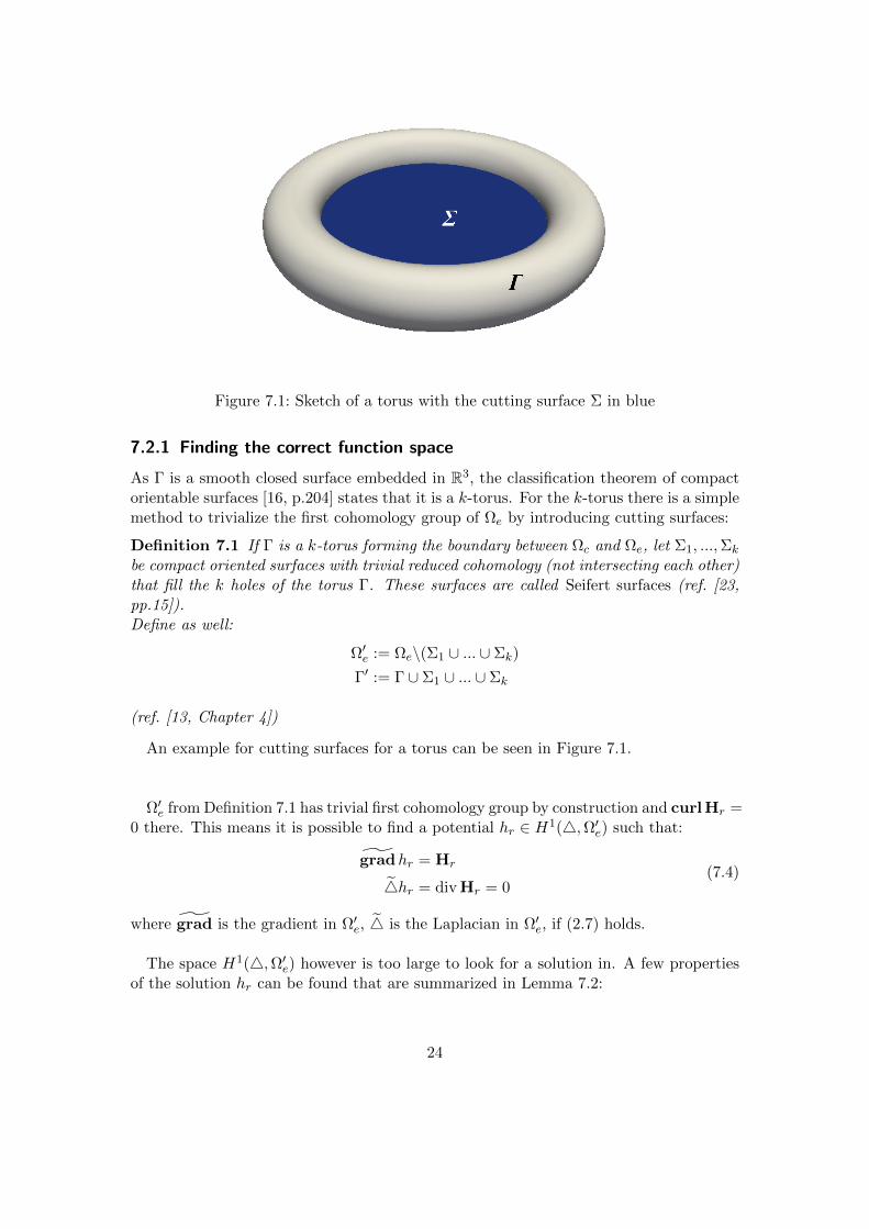
Figure 7.1: Sketch of a torus with the cutting surface Σ in blue

7.2.1 Finding the correct function space

As Γ is a smooth closed surface embedded in R3, the classification theorem of compactorientable surfaces [16, p.204] states that it is a k-torus. For the k-torus there is a simplemethod to trivialize the first cohomology group of Ωe by introducing cutting surfaces:

Definition 7.1 If Γ is a k-torus forming the boundary between Ωc and Ωe, let Σ1, ...,Σk

be compact oriented surfaces with trivial reduced cohomology (not intersecting each other)that fill the k holes of the torus Γ. These surfaces are called Seifert surfaces (ref. [23,pp.15]).Define as well:

Ω′e := Ωe\(Σ1 ∪ ... ∪ Σk)

Γ′ := Γ ∪ Σ1 ∪ ... ∪ Σk

(ref. [13, Chapter 4])

An example for cutting surfaces for a torus can be seen in Figure 7.1.

Ω′e from Definition 7.1 has trivial first cohomology group by construction and curl Hr =0 there. This means it is possible to find a potential hr ∈ H1(4,Ω′e) such that:

gradhr = Hr

4hr = div Hr = 0(7.4)

where grad is the gradient in Ω′e, 4 is the Laplacian in Ω′e, if (2.7) holds.

The space H1(4,Ω′e) however is too large to look for a solution in. A few propertiesof the solution hr can be found that are summarized in Lemma 7.2:

24

Lemma 7.2 The solution hr to (7.4) fulfills the following properties:

(i) The gradient gradhr is continuous along all the cutting surfaces.(ii) The function hr has a constant jump across each cutting surface.

Proof (i) The continuity of gradhr along cutting surfaces follows from the fact that

gradhr = Hr. The discussion in Chapter 2 of Hr as a physical quantity gives the con-tinuity of Hr in all of Ωe (not just Ω′e).

This also means that although hr ∈ H1(4,Ω′e) it holds that gradhr can be easily ex-

tended to H(curl; Ωe). From now on gradhr will always mean the extended, continuousversion in Ωe.

(ii) The constant jump of hr follows from Ampere’s law of magnetic fields. As of (2.7)it holds in all of Ωe:

curl gradhr = curl Hr = 0 (7.5)

This means by Stokes that for a closed curve C not passing through a cutting surface:∫C

gradhr(x) · t(x) dl(x) = 0 (7.6)

where t(x) is an appropriate tangent field. This is evident, as by the fundamentaltheorem of line integrals [22, Chapter 5.3] it should hold that:

hr(x2)− hr(x1) =

∫G

gradhr(x) · t(x) dl(x) (7.7)

where G is a curve from x1 to x2; thus at any point x where hr is continuous it musthold hr(x)− hr(x) = 0.

Consider now the points x+ε and x−ε which are at a distance of ε from the same point

x0 of the cutting surface, just above and just below. In the limit ε→ 0 the curve C fromx−ε to x+

ε (inside Ω′e, not along the cutting surface) is a closed curve in Ωe.Because C passes a cutting surface, Stokes and (7.5) do not hold, so the integral will besome quantity depending on the point of discontinuity:∫

Cgradhr(x) · t(x) dl(x) = I(x0) (7.8)

This function I signifies the jump of hr across the cutting surface, as (7.7) gives hr(x+ε )−

hr(x−ε ) = I(x0). In the electromagnetic context this is the current flowing inside the

torus.However I(x0) is independent of the chosen x0 on the cutting surface. Consider a secondpoint x′0 somewhere on the cutting surface. Then it holds:

I(x′0) = I(x0) +

∫G+

gradhr(x) · t(x) dl(x) +

∫G−

gradhr(x) · t(x) dl(x) (7.9)

25

where G+ is a path from x+ε′

to x+ε and G− is a path from x−ε to x−ε

′. As gradhr is

continuous across the cutting surface, the two additional integrals must cancel in thelimit ε→ 0.This means I(x′0) = I(x0). Thus the jump of hr across any cutting surface is constant.

This is consistent with [13, Chapter 4].

Lemma 7.2 motivates Definition 7.3:

Definition 7.3

H1Σ(Ω′e) := ϕ ∈ H1(4,Ω′e) | [γϕ]Σi = const, (∂nϕ)Σ+

i= −(∂nϕ)Σ−i

∀i

[f ]Σi is the jump of f across Σi.Σ+i is the “above part” of Σi oriented upwards and Σ−i is the “below part” of Σi oriented

downwards.The corresponding Dirichlet and Neumann trace spaces are:

H12Σ (Γ′) := v ∈ H

12 (Γ\ ∪i ∂Σi) | v ∈ H

12 (Σ+

i ), v ∈ H12 (Σ−i ), [v]Σi = const ∀i

H− 1

2Σ (Γ′) := v ∈ H−

12 (Γ\ ∪i ∂Σi) | v ∈ H−

12 (Σ+

i ), v ∈ H−12 (Σ−i ), v|Σ+

i= −v|Σ−i ∀i

Lemma 7.2 shows that hr must be in H1Σ(Ω′e): the constant jump in Dirichlet trace as

well as the continuity in the gradient (which leads to opposite Neumann traces due to theopposite orientation of normal vectors) come from Lemma 7.2. It is enough to test withthe appropriate test functions from this space in a weak formulation. This is beyondthe scope of this thesis; theory on this can be found in e.g. [1, Section 4], [13, Theorem 2].

7.2.2 Calderon identities

As discussed in Section 7.2, inside the conductor the normal Calderon identities hold.Outside the conductor however they do not hold; a modified version has to be used whichis derived from Green’s third identity (the representation formula).The calculations in this subsection are done just for the case of the torus (where thereis one cutting surface, Σ), but they easily extend to the general case.

Consider the cross-section of the torus with infinitesimally thin cutting surface dis-played in Figure 7.2. This model provides a closed, oriented surface Γ′ = Γ ∪ Σ+ ∪ Σ−

on which integral equations can be formulated.

The first Calderon identity in this model takes the form of Lemma 7.4:

26

Figure 7.2: Cross-section of a torus where the cutting surface Σ has been expanded to beinfinitesimally thick. Its above part is Σ+, its below part is Σ−. The wholesurface is Γ′ = Γ ∪ Σ+ ∪ Σ−.

Lemma 7.4 Let hr be the solution to (7.4).Let VS be the single layer operator over the surface S and KS the double layer operatorover the surface S. Then it holds:

γehr = −VΓ∂enhr +

(KΓ +

1

2

)γehr + [h]ΣKΣ+1 on Γ (7.10a)

γ+hr = −VΓ∂enhr +KΓγ

ehr + [h]Σ

(KΣ+1 +

1

2

)on Σ+ (7.10b)

γ−hr = −VΓ∂enhr +KΓγ

ehr + [h]Σ

(KΣ+1− 1

2

)on Σ− (7.10c)

Proof With G(x, y) being the Green’s kernel for the Laplace equation, Green’s thirdidentity is [9, p.712] (notice the changed signs, as in this formulation the normal vectorspoint outwards):

−hr(x) =

∫Γ′G(x, y)

∂

∂nyhr(y)dS(y)−

∫Γ′hr(y)

∂

∂nyG(x, y)dS(y), x /∈ Γ′ (7.11)

When taking the Dirichlet trace in the limit x→ x0 ∈ Γ, the equation becomes:

γehr(x0) = −∫

ΓG(x0, y)∂enhr(y)dS(y) +

∫Γγehr(y)∂enyG(x0, y)dS(y) +

1

2γehr(x0)

−∫

Σ+

G(x0, y)∂+n hr(y)dS(y)−

∫Σ−

G(x0, y)∂−n hr(y)dS(y) (these cancel)

+

∫Σ+

γ+hr(y)∂+n yG(x0, y)dS(y) +

∫Σ−

γ−hr(y)∂−n yG(x0, y)dS(y)

(7.12)

27

where the limit properties of the single and double layer potential [28, Chapter 6], [28,Lemma 6.7], [28, Lemma 6.11] have been used.The superscripts + and − to the trace operators mean the trace is taken from above orbelow the cutting surface (as notions of internal and external trace do not make senseon the cutting surface).Due to the constant jump property, γ−hr = γ+hr − [h]Σ. This gives:

γehr(x0) = −∫

ΓG(x0, y)∂enhr(y)dS(y) +

∫Γγehr(y)∂enyG(x0, y)dS(y) +

1

2γehr(x0)

+

∫Σ+

γ+hr(y)∂+n yG(x0, y)dS(y) +

∫Σ−

(γ+hr(y)− [h]Σ)∂−n yG(x0, y)dS(y)

= −∫

ΓG(x0, y)∂enhr(y)dS(y) +

∫Γγehr(y)∂enyG(x0, y)dS(y) +

1

2γehr(y)

+ [h]Σ

∫Σ+

∂+n yG(x0, y)dS(y)

(7.13)

In the operator notation this becomes:

γehr = −VΓ∂enhr +

(KΓ +

1

2

)γehr + [h]ΣKΣ+1 on Γ (7.14)

When taking the Dirichlet trace in the limit x→ x0 ∈ Σ+, the equation becomes:

γ+hr(x0) = −∫

ΓG(x0, y)∂enhr(y)dS(y) +

∫Γγehr(y)∂enyG(x0, y)dS(y)

−∫

Σ+

G(x0, y)∂+n hr(y)dS(y)−

∫Σ−

G(x0, y)∂−n hr(y)dS(y) (these cancel)

+

∫Σ+

γ+hr(y)∂+n yG(x0, y)dS(y) +

∫Σ−

γ−hr(y)∂−n yG(x0, y)dS(y)

+1

2γ+hr(x0)− 1

2γ−hr(x0)

= −∫

ΓG(x0, y)∂enhr(y)dS(y) +

∫Γγehr(y)∂enyG(x0, y)dS(y)

[h]Σ

∫Σ+

∂+n yG(x0, y)dS(y) +

1

2[h]Σ

(7.15)

Here the limit properties have to be used for the Σ+ and the Σ− part of the integral, asthey are infinitesimally close.With the operator notation from above:

γ+hr = −VΓ∂enhr +KΓγ

ehr + [h]Σ

(KΣ+1 +

1

2

)on Σ+ (7.16)

28

With a similar calculation for Σ− it holds:

γ−hr = −VΓ∂enhr +KΓγ

ehr − [h]Σ

(KΣ−1 +

1

2

)= −VΓ∂

enhr +KΓγ

ehr + [h]Σ

(KΣ+1− 1

2

)on Σ−

(7.17)

This proves the first Calderon identity.

The second Calderon identity in this model takes the form of Lemma 7.5

Lemma 7.5 Let hr be the solution to (7.4).Let DS be the hypersingular operator over the surface S and K∗S the adjoint double layeroperator over the surface S. Then it holds:

∂enhr =

(−K∗Γ +

1

2

)∂enhr −DΓγ

ehr − [hr]ΣDΣ+1 on Γ (7.18a)

∂+n hr = −K∗Γ∂enhr −DΓγ

ehr − [hr]ΣDΣ+1 + ∂+n hr on Σ+ (7.18b)

∂−n hr = −K∗Γ∂enhr −DΓγehr − [hr]ΣDΣ+1− ∂+

n hr on Σ− (7.18c)

Proof Again, start with Green’s third identity for the Green’s kernel G(x, y):

hr(x) = −∫

Γ′G(x, y)

∂

∂nyhr(y)dS(y) +

∫Γ′hr(y)

∂

∂nyG(x, y)dS(y), x /∈ Γ′ (7.19)

This time the Neumann trace is taken. In the limit x→ x0 ∈ Γ this yields:

∂enhr(x0) = −∫

Γ∂enxG(x0, y)∂enhr(y)dS(y) +

1

2∂enhr(x0) + ∂enx

∫Γγehr(y)∂enyG(x0, y)dS(y)

−∫

Σ+

∂enxG(x0, y)∂+n hr(y)dS(y)−

∫Σ−

∂enxG(x0, y)∂−n hr(y)dS(y)

+ ∂enx

∫Σ+

γ+hr(y)∂+n yG(x0, y)dS(y) + ∂enx

∫Σ−

γ−hr(y)∂−n yG(x0, y)dS(y)

= −∫

Γ∂enxG(x0, y)∂enhr(y)dS(y) +

1

2∂enhr(x0) + ∂enx

∫Γγehr(y)∂enyG(x0, y)dS(y)

+ [hr]Σ∂enx

∫Σ+

∂+n yG(x0, y)dS(y)

(7.20)

where again a limit property from [28, Chapter 6], namely [28, Lemma 6.8] was used.

29

In the operator notation this becomes:

∂enhr =

(−K∗Γ +

1

2

)∂enhr −DΓγ

ehr − [hr]ΣDΣ+1 on Γ (7.21)

When taking the Neumann trace in the limit x→ x0 ∈ Σ+ this is:

∂enhr(x0) = −∫

Γ∂+n xG(x0, y)∂enhr(y)dS(y) + ∂+

n x

∫Γγehr(y)∂enyG(x0, y)dS(y)

−∫

Σ+

∂+n xG(x0, y)∂+

n hr(y)dS(y)−∫

Σ−∂+n xG(x0, y)∂−n hr(y)dS(y)

+ ∂+n x

∫Σ+

γ+hr(y)∂+n yG(x0, y)dS(y) + ∂+

n x

∫Σ−

γ−hr(y)∂−n yG(x0, y)dS(y)

+1

2∂+n hr(x0)− 1

2∂−n hr(x0)

= −∫

Γ∂+n xG(x0, y)∂enhr(y)dS(y) + ∂+

n x

∫Γγehr(y)∂enyG(x0, y)dS(y)

+ [hr]Σ∂+n x

∫Σ+

∂+n yG(x0, y)dS(y) + ∂+

n hr(x0)

(7.22)

In the operator notation this becomes

∂+n hr = −K∗Γ∂enhr −DΓγ

ehr − [hr]ΣDΣ+1 + ∂+n hr on Σ+ (7.23)

By a similar calculation on Σ− it holds:

∂−n hr = −K∗Γ∂enhr −DΓγehr + [hr]ΣDΣ−1 + ∂−n hr on Σ−

= −K∗Γ∂enhr −DΓγehr − [hr]ΣDΣ+1− ∂+

n hr on Σ−(7.24)

7.2.3 Weak formulation

It remains to find a weak formulation for the Calderon identities described in the lastsubsection. As the spaces are dual to each other, the first Calderon identity from Lemma

30

7.4 is tested with a function ϕ from H− 1

2Σ (Γ′):

〈ϕ, γehr〉Γ′ = 〈ϕ, γehr〉Γ +⟨ϕ, γ+hr

⟩Σ+ +

⟨ϕ, γ−hr

⟩Σ−

=

⟨ϕ,−VΓ∂

enhr +

(KΓ +

1

2

)γehr + [h]ΣKΣ+1

⟩Γ

+

⟨ϕ,−VΓ∂

enhr +KΓγ

ehr + [h]Σ

(KΣ+1 +

1

2

)⟩Σ+

+

⟨ϕ,−VΓ∂

enhr +KΓγ

ehr + [h]Σ

(KΣ+1− 1

2

)⟩Σ−

=

⟨ϕ,−VΓ∂

enhr +

(KΓ +

1

2

)γehr + [h]ΣKΣ+1

⟩Γ

+ [h]Σ+ 〈ϕ, 1〉Σ+

〈ϕ, γehr〉Γ = −〈ϕ, VΓ∂enhr〉Γ +

⟨ϕ,

(KΓ +

1

2

)γehr

⟩Γ

+ [h]Σ 〈ϕ,KΣ+1〉Γ

〈ϕ, VΓ∂enhr〉Γ =

⟨ϕ,

(KΓ −

1

2

)γehr

⟩Γ

+ [h]Σ 〈ϕ,KΣ+1〉Γ

(7.25)

By the same duality reasoning, the second Calderon identity from Lemma 7.5 is tested

with a function v from H12Σ (Γ′):

〈v, ∂enhr〉Γ′ = 〈v, ∂enhr〉Γ +⟨v, ∂+

n hr⟩

Σ+ +⟨v, ∂−n hr

⟩Σ−

=

⟨v,

(−K∗Γ +

1

2

)∂enhr −DΓγ

ehr − [hr]ΣDΣ+1

⟩Γ

+⟨v,−K∗Γ∂enhr −DΓγ

ehr − [hr]ΣDΣ+1 + ∂+n hr

⟩Σ+

+⟨v,−K∗Γ∂enhr −DΓγ

ehr − [hr]ΣDΣ+1− ∂+n hr

⟩Σ−

〈v, ∂enhr〉Γ = −〈v,DΓγehr + [hr]ΣDΣ+1〉Γ +

⟨v,

(−K∗Γ +

1

2

)∂enhr

⟩Γ

− [v]Σ 〈1,K∗Γ∂enhr〉Σ+ − [v]Σ 〈1, DΓγehr + [hr]ΣDΣ+1〉Σ+

〈v,DΓγehr + [hr]ΣDΣ+1〉Γ + [v]Σ 〈1, DΓγ

ehr + [hr]ΣDΣ+1〉Σ+ =

−⟨v,

(K∗Γ +

1

2

)∂enhr

⟩Γ

− [v]Σ 〈1,K∗Γ∂enhr〉Σ+

(7.26)

7.2.4 Partial integration of the hypersingular operator

A minor issue which has to be addressed here is the formulation of the hypersingular op-erator. As the hypersingular operator involves two derivatives it can not be implementedthe way it is defined numerically. For the case of the method with simple geometriesthe hypersingular operator has been reduced to the single layer operator for vectors in

31

the bilinear setting (ref. (4.3) where it was assumed that the surface is closed and thefunctions continuous) using [28, Lemma 6.16] and [28, Theorem 6.17].However these do not hold for the case of discontinuous functions and non-closed sur-faces. In order to be able to implement the hypersingular operator these issues have tobe addressed.

The suitable modification for [28, Lemma 6.16] is Lemma 7.6:

Lemma 7.6 Γ′, Γ, Σ± as used in this chapter before. u ∈ H12Σ (Γ′) and v ∈H

− 12⊥ (curlΓ,Γ).

Then it holds:∫Γ

curlΓu(x) · v(x)dS(x) = −∫

Γu(x) curlΓ v(x)dS(x)− [u]Σ

∫Σ+

curlΣ+ v(x)dS(x)

Proof For reasonable extensions u and v to Ωe, by the reasoning of [28, Lemma 6.16]it holds∫

ΓcurlΓu(x) · v(x)dS(x) =

∫Γ

(curl(u(x)v(x))− u(x) curl v(x)) · n(x)dS(x)∫Γu(x) curlΓ v(x)dS(x) =

∫Γ

curl(u(x)v(x)) · n(x)dS(x)−∫

ΓcurlΓu(x) · v(x)dS(x)

(7.27)

Because of the discontinuity at the boundary of the cutting surface, applying Stokesgives:∫

Γcurl(u(x)v(x)) · n(x)dS(x) = −

∫∂Σ+

u(x)v(x) · t∂Σ+(x)dS(x)−∫∂Σ−

u(x)v(x) · t∂Σ−(x)dS(x)

= −[u]Σ

∫∂Σ+

v(x) · t∂Σ+(x)dS(x)

= −[u]Σ

∫Σ+

curlΣ+ v(x)dS(x)

(7.28)

where t is an appropriate tangent field. The change in sign comes from the fact that thecutting surfaces’ boundaries are oriented opposite to the “discontinuity boundaries” onΓ.This fact combined with (7.27) gives the statement of the lemma.

The following version of the Lemma is also necessary:

Lemma 7.7 Γ′, Γ, Σ± as used in this chapter before. u ∈ H12 (Γ′), f ∈ H

12Σ (Γ′) and

v ∈H− 1

2⊥ (curlΓ,Γ).

Then it holds:∫Γ

curlΓu(x)·(f(x)v(x))dS(x) = −∫

Γu(x) curlΓ(f(x)v(x))dS(x)−[f ]Σ

∫Σ+

curlΣ+(u(x)v(x))dS(x)

32

Proof Following the proof of Lemma 7.7 it is possible to arrive at the following identity:∫Γu(x) curlΓ(f(x)v(x))dS(x) =

∫Γ

curl(u(x)f(x)v(x)

)· n(x)dS(x)

−∫

ΓcurlΓu(x) · (f(x)v(x))dS(x)

(7.29)

Because of the discontinuity, this time of f , at the boundary (as in Lemma 7.6) itholds:∫

Γcurl

(u(x)f(x)v(x)

)· n(x)dS(x) = −[f ]Σ

∫Σ+

curlΣ+(u(x)v(x))dS(x) (7.30)

which gives the statement of the lemma.

The suitable modification for [28, Theorem 6.17] is Theorem 7.8:

Theorem 7.8 Γ′, Γ, Σ± as used in this chapter before. u ∈ H12Σ (Γ′).

Then it holds:

〈v,DΓu+ [u]ΣDΣ+1〉Γ + [v]Σ 〈1, DΓγeu+ [u]ΣDΣ+1〉Σ+

=

∫Γ

∫Γ

curlΓv(x) · curlΓu(y)G(x, y)dS(x)dS(y)

= 〈curlΓv,AΓcurlΓu〉Γ

where DS is the scalar hypersingular operator and AS is the vectorial single layer operator(for the Laplace equation) on the surface S.

Proof Let w(x) :=∫

Γ u(y)∂enG(x, y)dS(y) + [u]Σ∫

Σ+ ∂+nG(x, y)dS(y) where x ∈ Ωe,

x /∈ Γ.By the reasoning of [28, Theorem 6.17] it holds:

∂

∂xiw(x) =

∫Γu(y)curlΓy

(ei × grady G(x, y)

)dS(y)

+ [u]Σ

∫Σ+

curlΣ+y

(ei × grady G(x, y)

)dS(y)

(7.31)

where the ei are the unit vectors in R3.

Using Lemma 7.6 it then holds:

∂

∂xiw(x) = −

∫Γ

curlΓu(y) ·(ei × grady G(x, y)

)dS(y) (7.32)

33

Now it is again possible to follow the proof from [28, Theorem 6.17] to get the followinglimit x→ x ∈ Γ:

(DΓu+ [u]ΣDΣ+1) (x) = − limε→0

∫y∈Γ|x−y|≥ε

curlΓu(y) · curlΓxG(x, y)dS(y)(7.33)

When weakly testing with some v ∈ H12Σ (Γ), the following holds:

〈v,DΓu+ [u]ΣDΣ+1〉Γ = −∫

Γv(x) lim

ε→0

∫y∈Γ|x−y|≥ε

curlΓu(y) · curlΓxG(x, y)dS(y)dS(x)

= −∫

Γlimε→0

∫x∈Γ|x−y|≥ε

(v(x)curlΓu(y)) · curlΓxG(x, y)dS(x)dS(y)

(7.34)

Using Lemma 7.7 gives:

〈v,DΓu+ [u]ΣDΣ+1〉Γ =

∫Γ

limε→0

( ∫x∈Γ|x−y|≥ε

curlΓx (v(x)curlΓu(y))G(x, y)dS(x)

+ [v]Σ

∫x∈Σ+

|x−y|≥ε

curlΣ+x(G(x, y)curlΓu(y))dS(x)

)dS(y)

(7.35)

At the same time it holds:

〈1, DΓγeu+ [u]ΣDΣ+1〉Σ+ = −

∫Γ

limε→0

∫x∈Σ+

|x−y|≥ε

curlΓu(y) · curlΣ+xG(x, y)dS(x)dS(y)

= −∫

Γlimε→0

∫x∈Σ+

|x−y|≥ε

curlx (G(x, y)curlΓu(y)) · n(x)dS(x)dS(y)

(7.36)

by the same reasoning as in the proofs of Lemmas 7.6 and 7.7. This time however, thereis no sign flip when integrating over ∂Σ+ as the boundary is approached from inside Σ+

itself and not from Γ.

Combining the last two equations gives:

〈v,DΓu+ [u]ΣDΣ+1〉Γ + [v]Σ 〈1, DΓγeu+ [u]ΣDΣ+1〉Σ+

=

∫Γ

limε→0

∫x∈Γ|x−y|≥ε

curlΓx (v(x)curlΓu(y))G(x, y)dS(x)dS(y) (7.37)

34

Together with the identity curlΓx(v(x)curlΓyu(y)

)= curlΓxv(x) · curlΓyu(y) from

[28, p.136] this proves the theorem.

Theorem 7.8 can now be used to get a simpler statement of (7.26):

〈curlΓv,AΓcurlΓγehr〉Γ = −

⟨v,

(K∗Γ +

1

2

)∂enhr

⟩Γ

− [v]Σ 〈1,K∗Γ∂enhr〉Σ+ (7.38)

7.3 Combining inside and outside

As in Chapter 5, the equations for inside the conductor, (7.2) and (7.3), and the equa-tions for outside the conductor, (7.25) and (7.38), are now combined using the couplingproperty (5.12). This can be accomplished in two ways: using only the first Calderonidentity (the non-symmetric way) or using both Calderon identities (the symmetric way,as it is done in Chapter 5). Both ways will be investigated here.

7.3.1 The non-symmetric way

Inserting γctH = gradΓγehr + γetHs into (7.3) using the coupling property (5.12) gives

(where v ∈ H12Σ (Γ)):

1

τ〈∂enhr, v〉d +

1

τ〈γenHs, v〉d = 〈V, (Bκ + 0.5 id) γcNH〉l + 〈V,NκγctH〉l

〈∂enhr, v〉d + 〈γenHs, v〉d = τ 〈V, (Bκ + 0.5 id) γcNH〉l+ τ

⟨V,Nκ

(gradΓγ

ehr + γetHs

)⟩l

〈γenHs, v〉d − τ 〈V,NκγetHs〉l = τ

⟨V,NκgradΓγ

ehr

⟩l

+ τ 〈V, (Bκ + 0.5 id) γcNH〉l − 〈∂enhr, v〉d

〈v, γenHs〉d − τ⟨gradΓv,N

κγetHs

⟩l

= τ⟨gradΓv,N

κgradΓγehr

⟩l

+ τ⟨gradΓv, (B

κ + 0.5 id) γcNH⟩l− 〈v, ∂enhr〉d

(7.39)

where in the last line it was used that V = gradΓv, v ∈ H12Σ (Γ).

35

Inserting γctH = gradΓγehr + γetHs into (7.2) gives:

0 =⟨µ, (Cκ − 0.5 id)

(gradΓγ

ehr + γetHs

)⟩l+ 〈µ,AκγcNH〉l

〈µ, (0.5 id−Cκ) γetHs〉l =⟨µ, (Cκ − 0.5 id) gradΓγ

ehr

⟩l+ 〈µ,AκγcNH〉l

(7.40)

with µ ∈H− 1

2

|| (divΓ,Γ) as in (7.2).

Finally, (7.25) gives:

0 =

⟨ϕ,

(KΓ −

1

2

)γehr

⟩d

+ [h]Σ 〈ϕ,KΣ+1〉d − 〈ϕ, VΓ∂enhr〉d (7.41)

where ϕ ∈ H−12 (Γ).

7.3.2 The symmetric way

The symmetric version is obtained by using the second scalar Calderon identity (7.26)on the scalar Neumann trace in (7.39). The result is summed up in Theorem 7.9:

Theorem 7.9 The weak formulation of the symmetric boundary integral equations forthe eddy current problem are:

〈v, γenHs〉d − τ⟨gradΓv,N

κγetHs

⟩l

= τ⟨gradΓv,N

κgradΓγehr

⟩l

+ τ⟨gradΓv, (B

κ + 0.5 id) γcNH⟩l

+

⟨v,

(K∗Γ −

1

2

)∂enhr

⟩d

+ [v]Σ 〈KΣ+1, ∂enhr〉d+ 〈curlΓv,AΓcurlΓγ

ehr〉l

(7.42a)

〈µ, (0.5 id−Cκ) γetHs〉l =⟨µ, (Cκ − 0.5 id) gradΓγ

ehr

⟩l+ 〈µ,AκγcNH〉l (7.42b)

0 =

⟨ϕ,

(1

2−KΓ

)γehr

⟩Γ

− [h]Σ 〈ϕ,KΣ+1〉Γ + 〈ϕ, VΓ∂enhr〉Γ (7.42c)

where the unknowns are γehr ∈ H12Σ (Γ), ∂enhr ∈ H−

12 (Γ) and γcNH ∈H

− 12

|| (divΓ,Γ). and

the test functions are v ∈ H12Σ (Γ), µ ∈H

− 12

|| (divΓ,Γ) and ϕ ∈ H−12 (Γ).

36

Proof Inserting (7.26) into (7.39) gives the first equation:

〈v, γenHs〉d − τ⟨gradΓv,N

κγetHs

⟩l

= τ⟨gradΓv,N

κgradΓγehr

⟩l

+ τ⟨gradΓv, (B

κ + 0.5 id) γcNH⟩l

+

⟨v,

(K∗Γ −

1

2

)∂enhr

⟩d

+ [v]Σ 〈1,K∗Γ∂enhr〉d(Σ+)

+ 〈curlΓv,AΓcurlΓγehr〉l

〈v, γenHs〉d − τ⟨gradΓv,N

κγetHs

⟩l

= τ⟨gradΓv,N

κgradΓγehr

⟩l

+ τ⟨gradΓv, (B

κ + 0.5 id) γcNH⟩l

+

⟨v,

(K∗Γ −

1

2

)∂enhr

⟩d

+ [v]Σ 〈KΣ+1, ∂enhr〉d+ 〈curlΓv,AΓcurlΓγ

ehr〉l

(7.43)

The last two equations are just (7.40) and (7.41).

7.3.3 Dependence on the choice of cutting surface

It should be noted here that both formulations are completely independent of the choiceof the cutting surface Σ. The only relevant choice is the boundary of the cutting surface.This is because both formulations contain Σ only in integrals of the following type:

〈ϕ,KΣ+1〉Γ =

∫Γϕ(x)

∫Σ+

∂enyG(x, y)dS(y)dS(x) (7.44)

As the divergence of grady G(x, y) is 0 (except on a null set where Γ intersects Σ+)

for any other cutting surface Σ+′ with the same boundary oriented in the same way itholds by Gauss’s divergence theorem (ref. e.g. [22, Chapter 12]):

∫Σ+

∂enyG(x, y)dS(y)−∫

Σ+′∂enyG(x, y)dS(y) = 0∫

Σ+

∂enyG(x, y)dS(y) =

∫Σ+′

∂enyG(x, y)dS(y)

(7.45)

37

where the minus in the formulation comes from the fact that Σ+′ has to be oriented inthe context of Gauss’s theorem: the two surfaces have to form the closed boundary of avolume.

Thus the formulation is not dependent on how the cutting surface is chosen, only itsboundary matters. This is consistent with [13, pp.242].

38

8 Implementation of the method forcomplicated geometries

This chapter describes the implementation of the boundary element method for compli-cated geometries outlined in Chapter 7. First the discretization of the spaces is discussed,then the Calderon identities from Lemmas 7.4 and 7.5 are tested with a real-world ex-ample on a torus. At last the full eddy current problem on the torus is implemented.

As in Chapter 6 the actual implementations are done with BETL2 [20], meshing isdone with Gmsh [10] and visualization is done with Paraview [21].

In this section the domain in question will always be one where the conductor is atorus Γ with just one cutting surface Σ.

8.1 Discretization of the jump spaces

The discretization of the normal trace spaces H12 (Γ) and H−

12 (Γ) are discussed in Chap-

ter 6. However if the boundary integral equations from Lemmas 7.4 and 7.5 are to be

implemented it is necessary to discretize H12Σ (Γ′) restricted to Γ. The space H

− 12

Σ (Γ′)does not have to be implemented as it is discontinuous by nature and all parts on theactual cutting surface Σ vanish in the formulation of the Calderon identities.

Consider Definition 8.1:

Definition 8.1 Let ρ be a function in H12Σ (Γ′) with jump of 1 over the cutting surface

that integrates to 0.This function is called the ansatz function.

An example of such a function can be seen in Figure 8.1. The value of ρ on Σ is notrelevant, as this only enters the formulation via the jump of ρ over Σ. The value ofρ on Γ is important in the sense that the solution will depend on it; but the physicalquantities do not depend on the choice of ρ as will be apparent by construction.

These facts motivate the following ansatz (hence the name ansatz function for ρ):

γehr = u+ αρ u ∈ H12 (Γ), α ∈ C (8.1)

With this formulation u can be used with BETL2’s usual discretization of boundaryspaces and an additional degree of freedom, the jump α over the cutting surface, isintroduced (ρ is not an unknown).

39

Figure 8.1: An example for a possible choice of the ansatz function ρ. As the chosenvisualization method has some difficulties representing discontinuities, thepicture of the bottom shows artifacts that stem from this discontinuity. Thecalculation itself in BETL2 is not affected by this.

40

8.2 Testing the Calderon identities

The weak formulations of the Calderon identities applied to the ansatz (8.1) produce alinear system of equations for both identities.

8.2.1 Testing the first Calderon identity

(7.25) becomes:

〈ϕ, VΓψ〉d =

⟨ϕ,

(KΓ −

1

2

)(u+ αρ)

⟩d

+ α 〈ϕ,KΣ+1〉d

=

⟨ϕ,

(KΓ −

1

2

)u

⟩d

+ α

(⟨ϕ,

(KΓ −

1

2

)ρ

⟩d

+ 〈ϕ,KΣ+1〉d) (8.2)

where u ∈ H12 (Γ) is discussed above and ψ ∈ H−

12 (Γ) represents the Neumann trace of

hr on Γ. The test function is ϕ ∈ H−12 (Γ).

As BETL2 also offers integrals over discontinuous, piecewise linear spaces, (8.2) canbe implemented in the same framework as before. Using the notation from Chapter 6,the following matrices are formulated:

V 0 = Λ0SL(H(0Γ), H(0Γ)), V 0 ∈ Cn0×n0

K0 = Λ0DL(H(0Γ), H(1Γ)), K0 ∈ Cn0×n1

K0d = Λ0

DL(H(0Γ), H(1discΓ )), K0d ∈ Cn0×ndisc

K0s = Λ0

DL(H(0Γ), H(1Σ+)), K0d ∈ Cn0×n1,s

(8.3)

where a subscript denotes the surface on which the operator is formulated and a su-perscript 1disc means the space does not consist of continuous piecewise linears butdiscontinuous piecewise linears. All the discontinuous discretizations have ndisc degreesof freedom. n1,s is the dimension of the space H(1Σ+).

This gives the following matrix equation for (8.3):

V 0ψ =(K0 − 0.5M

)u+ α

((K0d − 0.5M

)ρ+ K0

s1)

(8.4)

where M is the respective mass matrix and 1 is a constant vector.

Consider now the physical setup of a constant current j0 along a wire loop on the in-side of the torus (such that the loop has constant distance to Γ) with constant minimaldistance from the torus surface Γ. This will produce a magnetic field in Ωe which willhave a potential hr in Ω′e obeying the Calderon identities.

The formula for such a magnetic field is known from [17, pp.181] which gives the Neu-mann trace. The potential hr along Γ is found using numerical quadrature. This means

41

Figure 8.2: A visualization of the calculated Neumann trace of the potential, ψ, on atorus with 2766 boundary elements.

number of bdryelements rel. error ψ

232 0.359274

784 0.226869

2766 0.0845532

10106 0.0538717

Table 8.1: L2 Errors of the method described in this chapter. ψ is compared to the exactNeumann trace known from [17, pp.181].

there is an exact solution to try (8.4) on.The method produces the correct solution and converges for an implementation of (8.4)with α = −j0 = −106, where the torus has a large radius of r1 = 0.5 and a small radiusof r2 = 0.1. A picture of the solution can be seen in 8.2, a convergence table can beseen in 8.1. The linear system was solved with Eigen’s partialPivLu [8]. The C++code that is used to produce the visualization is explained in the appendix in Section 11.7.

8.2.2 Testing the second Calderon identity

For the second identity that is tested with H12Σ (Γ) the setup is more intricate. In line

with the ansatz above it is sufficient to test with functions from H12 (Γ) as well as the

ansatz function ρ.

42

(7.38) tested with v ∈ H12 (Γ), becomes:

〈curlΓv,AΓcurlΓ(u+ αρ)〉l = −⟨v,

(K∗Γ +

1

2

)ψ

⟩d

〈curlΓv,AΓcurlΓu〉l + α 〈curlΓv,AΓcurlΓρ〉l = −⟨(

KΓ +1

2

)v, ψ

⟩d

(8.5)

(7.38) tested with ρ, becomes:

〈curlΓρ,AlcurlΓ(u+ αρ)〉Γ = −⟨ρ,

(K∗Γ +

1

2

)ψ

⟩d

− 〈1,K∗Γψ〉d(Σ+)

〈curlΓρ,AΓcurlΓu〉l + α 〈curlΓρ,AΓcurlΓρ〉l = −⟨(

KΓ +1

2

)ρ, ψ

⟩d

− 〈KΣ+1, ψ〉d(8.6)

The double layer operator is implemented as usual. The hypersingular operator isreplaced by the vectorial single layer operator (ref. Theorem 7.8) and implemented asfollowing:

D0 = GTc Λ0SL(H(divΓ), H(divΓ))Gc, D0 ∈ Cn1×n1

D0d = GTc Λ0

SL(H(divΓ), H(divdiscΓ ))Gdiscc D0d ∈ Cn1×ndisc

D0dd = Gdiscc

TΛ0SL(H(divdiscΓ ), H(divdiscΓ ))Gdiscc D0

dd ∈ Cndisc×ndisc

(8.7)

where Gc is the combinatorial curl as used in Chapter 6 and Gdiscc its version on dis-continuous spaces. Those are also matrices and their sizes correspond to the respectivedegrees of freedom of the element spaces.

Written as a matrix equation, (8.6) becomes:(D0 D0

dρ

ρT D0dT ρT D0

ddρ

)(uα

)=

(−(K0T + 0.5M)ψ

−ρT (K0dT + 0.5M)ψ − ψT K0

s1

)(8.8)

as the hypersingular operator is self-adjoint (this can be seen from its definition in [28,Chapter 6.5]).

The solution on Γ is reclaimed as u+ αρ.

The same test as in the last subsection can be performed here. As before, a stabi-lization condition is needed so that u integrates to 0. This has not been successfullyimplemented so far. It is however important and should be addressed in future work.

8.3 The eddy current problem

No convenient exact solution is available for the full eddy current problem. However,the correctness of the Calderon identities checked in the last section instills confidencein the correctness of the method for eddy current problems as well.

43

8.3.1 The non-symmetric way

This subsection investigates the implementation of the non-symmetric equations (7.39),(7.40) and (7.41).

Consider the usual ansatz (the C++ code used for the implementation of the ansatzfunction is explained in the appendix in Section 11.6):

γehr = u+ αρ, u ∈ H12 (Γ)

∂enhr = ψ, ψ ∈ H−12 (Γ)

γcNH = η, η ∈H− 1

2

|| (divΓ,Γ)

Denote the boundary conditions from the exciting field by (the C++ code used for theincorporation of the boundary conditions also is explained in the appendix in Section11.6):

δ = γetHs

ν = γenHs

(7.39) becomes, tested with v ∈ H12 (Γ):

〈v, ν〉d − τ 〈gradΓ v,Nκδ〉l =

τ 〈gradΓ v,Nκ gradΓ u〉l + ατ

⟨gradΓ v,N

κgradΓρ⟩l

+ τ 〈gradΓ v, (Bκ + 0.5 id) η〉l − 〈v, ψ〉d

(8.9)

Tested with ρ it becomes:

〈ρ, ν〉d − τ⟨gradΓρ,N

κδ⟩l

=

τ⟨gradΓρ,N

κ gradΓ u⟩l+ ατ

⟨gradΓρ,N

κgradΓρ⟩l

+ τ⟨gradΓρ, (B

κ + 0.5 id) η⟩l− 〈ρ, ψ〉d

(8.10)

(7.40) becomes, tested with µ ∈H− 1

2

|| (divΓ,Γ):

〈µ, (0.5 id−Cκ) δ〉l = 〈µ, (Cκ − 0.5 id) gradΓ u〉l + α⟨µ, (Cκ − 0.5 id) gradΓρ

⟩l

+ 〈µ,Aκη〉l(8.11)

44

(7.41) becomes, tested with ϕ ∈ H−12 (Γ):

0 =

⟨ϕ,

(KΓ −

1

2

)u

⟩d

+ α

⟨ϕ,

(KΓ −

1

2

)ρ

⟩d

+ α 〈ϕ,KΣ+1〉d − 〈ϕ, VΓψ〉d (8.12)

As a matrix equation this becomes:N −τCT −M N

C Aκ 0 C

−K 0 −V 0 −K

NT −τCT −ρTM N′

uηψα

fg0

f

(8.13)

with M the appropriate mass matrix and the bold letters defined as following:

N := τGTg NκGg

N := τGTg Nκ(gradΓρ)

N′ := τ(gradΓρ)T Nκ(gradΓρ)

C := (Cκ − 0.5M)Gg

C := (Cκ − 0.5M)(gradΓρ)

K := 0.5M − K0

K := (0.5M − K0d)ρ− K0

s1

f = Mν − τGTg Nκδ

f = ρTMν − τ(gradΓρ)T Nκδ

g = (0.5M − Cκ)δ

(8.14)

where the BETL2 operators have either been defined in Chapter 6 or in this chapter.

The results can be seen in Figure 8.3. The linear system was solved with Eigen’spartialPivLu [8]. The C++ code that is used to produce the visualization is explainedin the appendix in Section 11.7. The parameters are wire coil radius b = 0.07, currentalong wire coil j0 = 106, torus large radius r1 = 0.05, torus small radius r2 = 0.01.

Note that the result is independent of the choice of cutting surface, as the two differentcutting surfaces of Figure 8.3 demonstrate. This is consistent with the physics of theproblem, as the cutting surface has no physical significance but is just a mathematicaltool to solve the problem. This mathematical fact is shown in Subsection 7.3.3.

8.3.2 The symmetric way

This subsection describes the implementation of the symmetric equations from Theorem7.9.

45

Figure 8.3: The top picture shows the real part of the scalar potential on the torus withtwo different cutting surfaces, the bottom picture shows the real part of thereaction field Hr on the torus with two different cutting surfaces. The resultsare independent of the choice of cutting surface.

46

The first equation, tested with v ∈ H12 (Γ), becomes:

〈v, ν〉d − τ 〈gradΓ v,Nκδ〉l = τ 〈gradΓ v,N

κ gradΓ u〉l + ατ⟨gradΓ v,N

κgradΓρ⟩l

+ τ 〈gradΓ v, (Bκ + 0.5 id) η〉l +

⟨v,

(K∗Γ −

1

2

)ψ

⟩d

+ 〈curlΓv,AΓcurlΓu〉l + α⟨curlΓv,AΓcurlΓρ

⟩l

(8.15)

The first equation, tested with ρ, becomes:

〈ρ, ν〉d − τ⟨gradΓρ,N

κδ⟩l

= τ⟨gradΓρ,N

κ gradΓ u⟩l+ ατ

⟨gradΓρ,N

κgradΓρ⟩l

+ τ⟨gradΓρ, (B

κ + 0.5 id) η⟩l+

⟨ρ,

(K∗Γ −

1

2

)ψ

⟩d

+⟨curlΓρ,AΓcurlΓu

⟩l+ α

⟨curlΓρ,AΓcurlΓρ

⟩l

+ 〈KΣ+1, ψ〉d(8.16)

The second equation, tested with µ ∈H− 1

2

|| (divΓ,Γ), becomes:

〈µ, (0.5 id−Cκ) δ〉l = 〈µ, (Cκ − 0.5 id) gradΓ u〉l + α⟨µ, (Cκ − 0.5 id) gradΓρ

⟩l

+ 〈µ,Aκη〉l(8.17)

The third equation, tested with ϕ ∈ H−12 (Γ), becomes:

0 =

⟨ϕ,

(1

2−KΓ

)u

⟩Γ

+ α

⟨ϕ,

(1

2−KΓ

)ρ

⟩Γ

− α 〈ϕ,KΣ+1〉Γ + 〈ϕ, VΓψ〉Γ (8.18)

As a matrix equation this becomes:N −CT −KT N

C τAκ 0 C

K 0 V 0 K

NT −CT −KT N′

uηψα

fg0

f

(8.19)

47

with M the appropriate mass matrix and the bold letters defined as following:

N := τGTg NκGg + D0

N := τGTg Nκ(gradΓρ) + D0

dρ

N′ := τ(gradΓρ)T Nκ(gradΓρ) + ρT D0ddρ

C := τ(Cκ − 0.5M)Gg

C := τ(Cκ − 0.5M)(gradΓρ)

K := 0.5M − K0

K := (0.5M − K0d)ρ− K0

s1

f = Mν − τGTg Nκδ

f = ρTMν − τ(gradΓρ)T Nκδ

g = τ(0.5M − Cκ)δ

(8.20)

As the second Calderon identity from Subsection 8.2.2 has not been implementedsuccessfully it is not reasonable implement the symmetric formulation at this point.This is, however, a goal for future work.

48

9 Removing the cutting surfaces

In Chapters 7 and 8 a method for general geometries was formulated. However, forthe case with nontrivial first cohomology group of Ωe the cutting surface Σ has to beintroduced. It serves no physical purpose and there is a lot of freedom in choosing it –it is arbitrary to a certain degree as shown in Subsection 7.3.3.This suggests that they can somehow be avoided completely in the formulation of themethod. This chapter deals with removing integrals over Σ from the formulation inChapters 7 and 8 entirely.

9.1 Theory

The integral that has to be simplified is:⟨u,K0

Σ+1⟩d

=

∫Γ

∫Σ+

∂+nyG0(x, y)u(x)dS(y)dS(x) (9.1)

As they will be frequently used in this chapter, boundary cycles are defined here:

Definition 9.1 Let Σ+ be the cutting surface oriented upwards as used in previous chap-ters. Define:

c := ∂Σ+ (9.2)

Those are the boundaries of the cutting surfaces. They are boundary cycles in the firsthomology group of Γ of which the cohomology group is the dual. As the cutting surfacescan be varied, the cycles can also be replaced by any other homologous cycle.

The double layer potential can not be reduced to c using Stokes’s theorem, as grady G0(x, y)has no vector potential but only a scalar potential. Let it be at first assumed that x /∈ Σ.This holds almost everywhere, except for the points where Σ is connected to Γ.

The gradient of the kernel grady G0(x, y) is just the electric field at y generated by apoint charge of −1 at x. This allows the following theorem to be used:

Theorem 9.2 Let e be an electrostatic point charge and E(x) the electric field it gener-ates.Let S be a surface separated from the charge e by a hyperplane.1

1This is not a harsh restriction. In most cases it should be possible to choose the surface like that.

49

e

S

C∂B

Cw

Cw

Br

Figure 9.1: A sketch of the cone construction used in the proof of Theorem 9.2

Let Ψ be the solid angle of the boundary of S over the point of the charge. The solidangle is a generalization of the 2D angle to R3. It is the area on the unit sphere coveredby the projection of a surface onto the unit sphere (ref. [29]), or as in this case, the areacircumscribed by the projection of a curve onto the unit sphere.Then it holds: ∫

Sn(x) ·E(x) dsx =

Ψ

4πe

Proof Assume the charge and the surface are separated by some hyperplane H ∈ R3.Consider a ball Br with radius r > 0 centered around the charge e fully contained

in the charge’s half-space. There is a cone C of ∂S over the position of the charge e.Without loss of generality, the cone does not intersect S except at ∂S (the same argumentholds even with intersections, but is more cumbersome). Where the cone intersects theball Br it forms a surface C∂B with area Ψr2. The side of the cone up to the intersectionwith Br is called Cw. A sketch of the situation can be seen in Figure 9.1.

For notational convenience, the volume contained by C∂B, Cw and S is called V .

Now, Gauss’s electric field law (ref. [11, pp.67] which uses different scaling) states thatthe electric flux surface over a closed surface is just the sum of all charges enclosed by

50

the surface. This gives: ∫∂Br

n(x) ·E(x) dS(x) = e (9.3)

Thus, because of symmetry:∫C∂B

n(x) ·E(x) dS(x) =Ψr2

4πr2e =

Ψ

4πe (9.4)

Because V contains no charges, clearly the flux integral over ∂V is 0. Also, because ofhow the cone was constructed, all field lines of E are parallel to Cw. This leads to theflux integral of the field over the surface Cw being 0. This gives:

0 =

∫∂V

n(x) ·E(x) dsx =

(−∫C∂B

+

∫Cw

+

∫S

)n(x) ·E(x) dS(x)∫

Sn(x) ·E(x) dS(x) =

∫C∂B

n(x) ·E(x) dS(x) =Ψ

4πe

(9.5)

(note: the first minus sign is due to different orientation of C∂B depending on whichvolume it bounds)

This proves the theorem.2

This reduces the integral in (9.1) to the following integral:⟨u,K0

Σ+1⟩d

= − 1

4π

∫Γ

Ψc(x)u(x)dS(x) (9.6)

where ΨL(x) is the solid angle created by the loop L over the point x.

It remains to handle the cases where x = y can not be disregarded. This will onlyoccur on the intersection of Σ+ and Γ. This is a null set, so it will not matter in thesecond integration.

With these simplifications, the whole method has been reduced to just evaluationson Γ and the boundary of the cutting surface, c, whose dual cocycles generate the firstcohomology group of Ωe. This is highly relevant; there are efficient algorithms for thecomputation of these cycles, (as can be seen e.g. in [15]). Those algorithms are lessexpensive than constructing the whole cutting surface.

The same properties as in Chapter 8 still hold, as all the operators are still the samemathematically. There might be numerical issues which depend on how the solid angleis implemented.

2Some ideas for this proof come from a conversation with Nicolaus Heuer [12].

51

9.2 Algorithm

The only part of last section’s method of removing cutting surfaces that requires analgorithm that is not already used in this thesis is the calculation of the solid angle ofa point over a cutting surface. To that end, a simple algorithm will be proposed in thissection.

It is assumed that the input corresponding to the boundary cycle c is a polygon c

approximating c given in the form of a list of vertices. It is also assumed that thepoint over which the solid angle is formed is 0 (otherwise a simple translation has tobe made). Then the polygon can be projected onto the sphere with the algorithm fromCode Snippet 9.1.

1 f o r each ver tex v in c do :2 v := v/norm( v )3 end f o r

Code Snippet 9.1: Projecting the boundary of the cutting surface to the unit sphere

It remains to calculate the area enclosed by the projected polygon. This is the solidangle. Multiple approaches exist for this. If the polygon is convex there is a simplealgorithm depending only on the enclosed angles (where the formula is taken from [30]).It can be seen in Code Snippet 9.2.

1 ang l e s := 02 nVer t i c e s := 03 f o r each ver tex v in c do :4 ang l e s += enclosedAngleAt ( v )5 nVer t i c e s += 16 end f o r7 area := ( ang l e s − ( nVert ices −2)∗Pi )

Code Snippet 9.2: Calculating the area of the projected cutting surface

If the resulting polygon is non-convex, [6] has appropriate algorithms to calculate thearea enclosed by a polygon on a sphere in the general case.

52

10 Conclusion

This chapter will wrap up the master’s thesis, repeating its most important points andproduce an outlook on what further work can be done.

This master’s thesis introduced the magnetic field scalar potential approach for solvingquasi-stationary eddy current problems outlined in [13]. The approach solves the internalproblem using the normal vectorial Maxwell equations and vectorial boundary elementmethods. The external problem is solved as a scalar Laplace equation using scalarboundary element methods.

The theory was formulated for objects with simple geometries using standard scalarpotentials and then for more intricate geometries using discontinuous scalar potentials.The scalar potentials depend on cutting surfaces for more intricate geometries which areused to trivialize the first cohomology group of the nonconductive region Ωe.

Then boundary integral equations were formulated and simulated using BETL2 [20]for the sphere as well as for the torus. For the sphere a symmetric coupling was used,for the torus a symmetric and a non-symmetric coupling were derived but only the non-symmetric one was implemented.The results conform to the correct exact solutions where available.

Additionally, it was shown that the method is not only independent of the chosen cut-ting surfaces for complicated geometries, but that the method can be formulated to notneed any calculation on the cutting surfaces whatsoever. Chapter 9 reduces the wholemethod to boundaries of cutting surfaces only. These boundaries can be calculated inreasonable time using established algorithms.

Further work should mainly focus on the symmetric coupling for complicated geome-tries. The implementation of the second Calderon identity for complicated geometries(8.8) has not been successfully completed yet. A correct implementation of (8.8) inBETL2 is needed. This would also allow a realization of the full symmetric couplingmethod for the eddy current problem on the torus as it is formulated in (8.19).

53

11 Appendix

The appendix consists mostly of code snippets that illustrate the way the operators usedin this thesis are actually implemented in BETL2 using C++ code. The appendix itselfprovides only little context, but the different code snippets are referenced throughoutthe main body of the thesis.

The BETL2 revision used for the code is 73355M.1

All codes in this section are heavily influenced by the examples included in BETL2[20] and often directly taken from included applications. The examples are written eitherby Dr. Lars Kielhorn [19] or Elke Spindler [27]. Calculus and vector calculus identitiesneeded are common knowledge from [22] or [11, Back matter].

11.1 Implementation of finite element spaces

BETL2 offers four basic finite element space types that are used in this thesis. Linear andconstant Lagrangian elements (scalar) and curl- and div-type edge elements (vectorial).All the piecewise linear finite element spaces can be implemented as continuous (whichassigns only one degree of freedom for each edge or vertex) or discontinuous (whichassigns each edge or vertex multiple degrees of freedom, one for each adjacent triangle).

The finite element spaces are set up by first defining a finite element basis type,then defining a type for the DofHandler (where Dof stands for degrees of freedom),instantiating the DofHandler and then distribute the dofs for some grid structure. Acode example for this is provided in Code Snippet 11.1.

1 // s e t up element spaces2 typede f f e : : FEBasis< f e : : Linear , f e : : FEBasisType : : Lagrange >

f e b a s i s l a g r a n g e 1 t ;3 typede f f e : : FEBasis< f e : : Constant , f e : : FEBasisType : : Lagrange >

f e b a s i s l a g r a n g e 0 t ;4 typede f f e : : FEBasis< f e : : Linear , f e : : FEBasisType : : Div >

f e b a s i s d i v t ;5 typede f f e : : FEBasis< f e : : Linear , f e : : FEBasisType : : Curl >

f e b a s i s c u r l t ;6

1In the kernel integration routine, the scalar multiplication function of vectors has to be set to do anormal scalar multiplication, not a complex one.

54

7 // s e t up do fhand l e r s8 typede f f e : : DofHandler< f e b a s i s l a g r a n g e 1 t ,

f e : : FESContinuity : : Continuous , g r i d f a c t o r y t >d o f h a n d l e r l a g ra n g e 1 t ;

9 typede f f e : : DofHandler< f e b a s i s l a g r a n g e 1 t ,f e : : FESContinuity : : Discont inuous , g r i d f a c t o r y t >d o f h a n d l e r l a g r a n g e 1 d i s c o n t i n t ;

10 typede f f e : : DofHandler< f e b a s i s l a g r a n g e 0 t ,f e : : FESContinuity : : Discont inuous , g r i d f a c t o r y t >d o f h a n d l e r l a g ra n g e 0 t ;

11 typede f f e : : DofHandler< f e b a s i s d i v t ,f e : : FESContinuity : : Continuous , g r i d f a c t o r y t > d o f h a n d l e r d i v t ;

12 typede f f e : : DofHandler< f e b a s i s d i v t ,f e : : FESContinuity : : Discont inuous , g r i d f a c t o r y t >d o f h a n d l e r d i v d i s c o n t i n t ;

13 typede f f e : : DofHandler< f e b a s i s c u r l t ,f e : : FESContinuity : : Continuous , g r i d f a c t o r y t > d o f h a n d l e r c u r l t ;

14 typede f f e : : DofHandler< f e b a s i s c u r l t ,f e : : FESContinuity : : Discont inuous , g r i d f a c t o r y t >d o f h a n d l e r c u r l d i s c o n t i n t ;

15

16 // i n s t a n t i a t e do fhand l e r s17 d o f h a n d l e r l a g ra n g e 1 t do fhand l e r l ag range1 ;18 d o f h a n d l e r l a g r a n g e 1 d i s c o n t i n t d o f h a n d l e r l a g r a n g e 1 d i s c o n t i n ;19 d o f h a n d l e r l a g ra n g e 0 t do fhand l e r l ag range0 ;20 d o f h a n d l e r d i v t do fhand l e r d iv ;21 d o f h a n d l e r d i v d i s c o n t i n t d o f h a n d l e r d i v d i s c o n t i n ;22 d o f h a n d l e r c u r l t d o f h a n d l e r c u r l ;23 d o f h a n d l e r c u r l d i s c o n t i n t d o f h a n d l e r c u r l d i s c o n t i n ;24

25 // d i s t r i b u t e do f s26 do fhand l e r l ag range1 . d i s t r i b u t e D o f s ( g r i d f a c t o r y ) ;27 d o f h a n d l e r l a g r a n g e 1 d i s c o n t i n . d i s t r i b u t e D o f s ( g r i d f a c t o r y ) ;28 do fhand l e r l ag range0 . d i s t r i b u t e D o f s ( g r i d f a c t o r y ) ;29 do fhand l e r d iv . d i s t r i b u t e D o f s ( g r i d f a c t o r y ) ;30 d o f h a n d l e r d i v d i s c o n t i n . d i s t r i b u t e D o f s ( g r i d f a c t o r y ) ;31 d o f h a n d l e r c u r l . d i s t r i b u t e D o f s ( g r i d f a c t o r y ) ;32 d o f h a n d l e r c u r l d i s c o n t i n . d i s t r i b u t e D o f s ( g r i d f a c t o r y ) ;

Code Snippet 11.1: The process needed to set up finite element spaces and distributethe degrees of freedom in BETL2 for a grid with structure saved ingrid factory

To formulate certain operators only on parts of the grid (as it is done when usingcutting surfaces in Chapter 8), those surfaces have to be marked in the mesh file usingGmsh physical surfaces. The class MultiInterface handles the reading of the Gmshmarkings, and the extracting of the actual FE subspaces is shown in Code Snippet 11.2.

55

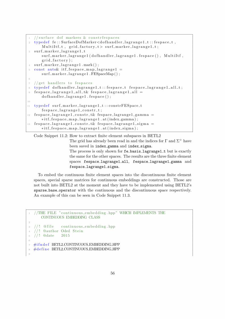
1 // s u r f a c e dof markers & c o n s t r f e s p a c e s2 typede f f e : : SurfaceDofMarker<d o f h a nd l e r l a g ra n g e 1 t : : f e s pac e t ,

M u l t i I t f t , g r i d f a c t o r y t> su r f marke r l ag range1 t ;3 su r f marke r l ag rang e1 t

sur f marke r l ag range1 ( do fhand l e r l ag range1 . f e s pa c e ( ) , Mu l t i I t f ,g r i d f a c t o r y ) ;

4 su r f marke r l ag range1 . mark ( ) ;5 const auto& i t f f e s p a c e m a p l a g r a n g e 1 =

sur f marke r l ag range1 . FESpaceMap ( ) ;6

7 // get hand le r s to f e s p a c e s8 typede f do f h a n d l e r l a g ra n g e 1 t : : f e s p a c e t f e s p a c e l a g r a n g e 1 a l l t ;9 f e s p a c e l a g r a n g e 1 a l l t& f e s p a c e l a g r a n g e 1 a l l =

do fhand l e r l ag range1 . f e s pa c e ( ) ;10

11 typede f su r f marke r l ag rang e1 t : : constrFESpace tf e s p a c e l a g r a n g e 1 c o n s t r t ;

12 f e s p a c e l a g r a n g e 1 c o n s t r t& fespace lagrange1 gamma =∗ i t f f e s p a c e m a p l a g r a n g e 1 . at ( index gamma ) ;

13 f e s p a c e l a g r a n g e 1 c o n s t r t& f e space l ag range1 s i gma =∗ i t f f e s p a c e m a p l a g r a n g e 1 . at ( index s igma ) ;

Code Snippet 11.2: How to extract finite element subspaces in BETL2The grid has already been read in and the indices for Γ and Σ+ havebeen saved in index gamma and index sigma.The process is only shown for fe basis lagrange1 t but is exactlythe same for the other spaces. The results are the three finite elementspaces fespace lagrange1 all, fespace lagrange1 gamma andfespace lagrange1 sigma.

To embed the continuous finite element spaces into the discontinuous finite elementspaces, special sparse matrices for continuous embeddings are constructed. Those arenot built into BETL2 at the moment and they have to be implemented using BETL2’ssparse base operator with the continuous and the discontinuous space respectively.An example of this can be seen in Code Snippet 11.3.

1 //THE FILE ”continuous embedding . hpp ” WHICH IMPLEMENTS THECONTINUOUS EMBEDDING CLASS

2

3 // ! @ f i l e continuous embedding . hpp4 // ! @author Oded Ste in5 // ! @date 20156

7 #i f n d e f BETL2 CONTINUOUS EMBEDDING HPP8 #d e f i n e BETL2 CONTINUOUS EMBEDDING HPP9

56

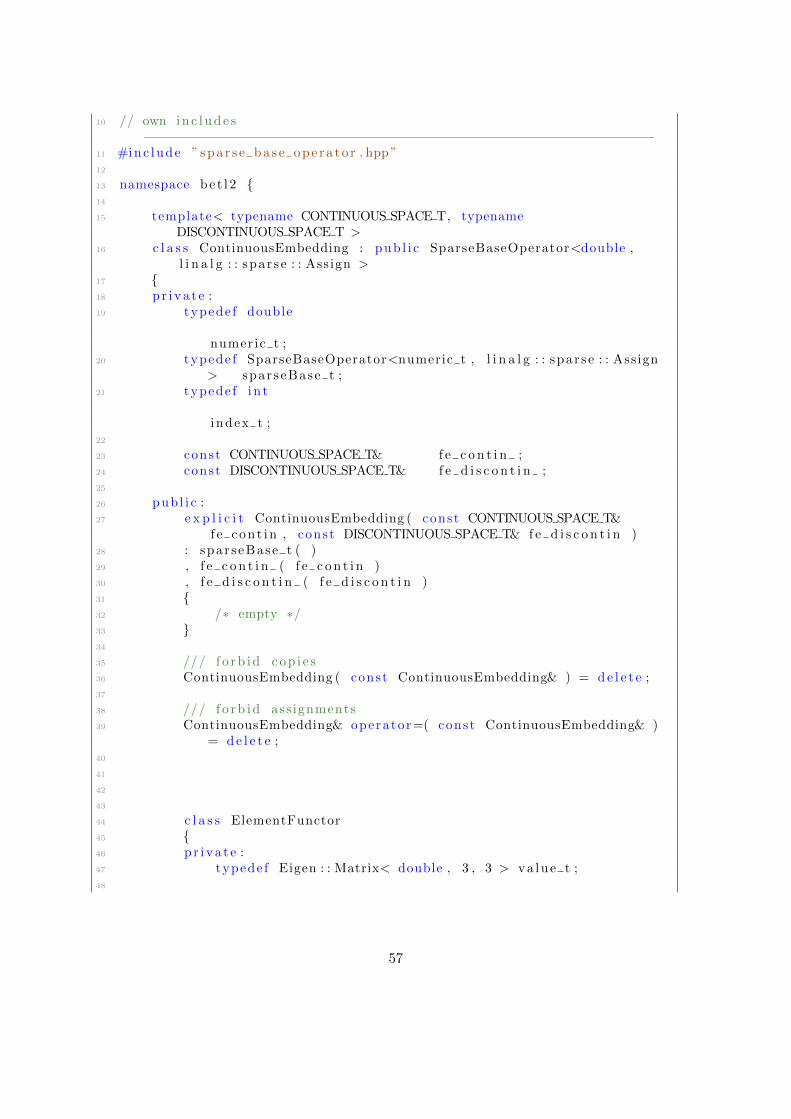
10 // own i n c l u d e s−−−−−−−−−−−−−−−−−−−−−−−−−−−−−−−−−−−−−−−−−−−−−−−−−−−−−−−−−−−−−−−−

11 #inc lude ”s p a r s e b a s e o p e r a t o r . hpp ”12

13 namespace b e t l 2 14

15 template< typename CONTINUOUS SPACE T, typenameDISCONTINUOUS SPACE T >

16 c l a s s ContinuousEmbedding : pub l i c SparseBaseOperator<double ,l i n a l g : : spa r s e : : Assign >

17 18 p r i v a t e :19 typede f double

numeric t ;20 typede f SparseBaseOperator<numeric t , l i n a l g : : spa r s e : : Assign

> spar seBase t ;21 typede f i n t

index t ;22

23 const CONTINUOUS SPACE T& f e c o n t i n ;24 const DISCONTINUOUS SPACE T& f e d i s c o n t i n ;25

26 pub l i c :27 e x p l i c i t ContinuousEmbedding ( const CONTINUOUS SPACE T&

f e c o n t i n , const DISCONTINUOUS SPACE T& f e d i s c o n t i n )28 : spa r s eBase t ( )29 , f e c o n t i n ( f e c o n t i n )30 , f e d i s c o n t i n ( f e d i s c o n t i n )31 32 /∗ empty ∗/33 34

35 /// f o r b i d c o p i e s36 ContinuousEmbedding ( const ContinuousEmbedding& ) = d e l e t e ;37

38 /// f o r b i d ass ignments39 ContinuousEmbedding& operator=( const ContinuousEmbedding& )

= d e l e t e ;40

41

42

43

44 c l a s s ElementFunctor45 46 p r i v a t e :47 typede f Eigen : : Matrix< double , 3 , 3 > va lue t ;48

57

49 pub l i c :50 ElementFunctor ( )51 /∗ empty ∗/ 52

53

54 template< typename ELEMENT ENTITY T >55 va lue t operator ( ) ( const ELEMENT ENTITY T& E ) const56 57 va lue t r e s u l t ;58 r e s u l t . s e t I d e n t i t y ( ) ;59

60 re turn r e s u l t ;61 62

63 ;64

65 pub l i c :66 template< typename RUNTIME CACHE T >67 void compute ( const RUNTIME CACHE T& runtime cache )68 69 const ElementFunctor e f ;70 t h i s −> a s s e m b l e T r i p l e t s ( f e c o n t i n , f e d i s c o n t i n , e f

) ;71 t h i s −> make sparse ( ) ;72 73 ; // end c l a s s ContinuousEmbedding74

75 // end namespace b e t l 276

77

78

79

80 //IMPLEMENTATION OF THE CONTINUOUS EMBEDDING81 typede f ContinuousEmbedding< f e s p a c e l a g r a n g e 1 c o n s t r t ,

f e s p a c e l a g r a n g e 1 d i s c o n t i n c o n s t r t >lagrange1 continuous embedding gamma op t ;

82 lagrange1 continuous embedding gamma op tlagrange1 continuous embedding gamma op ( fespace lagrange1 gamma ,f e space lagrange1 d i scont in gamma ) ;

83 lagrange1 continuous embedding gamma op . compute ( cache ) ;84 const auto& lag1 contin emb gamma =

lagrange1 continuous embedding gamma op . matrix ( ) ;

58

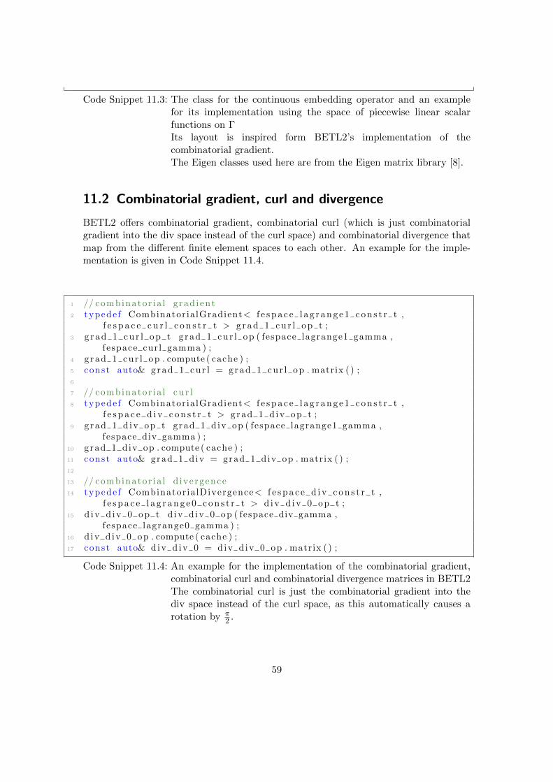
Code Snippet 11.3: The class for the continuous embedding operator and an examplefor its implementation using the space of piecewise linear scalarfunctions on ΓIts layout is inspired form BETL2’s implementation of thecombinatorial gradient.The Eigen classes used here are from the Eigen matrix library [8].

11.2 Combinatorial gradient, curl and divergence

BETL2 offers combinatorial gradient, combinatorial curl (which is just combinatorialgradient into the div space instead of the curl space) and combinatorial divergence thatmap from the different finite element spaces to each other. An example for the imple-mentation is given in Code Snippet 11.4.

1 // combinator ia l g rad i ent2 typede f CombinatorialGradient< f e s p a c e l a g r a n g e 1 c o n s t r t ,

f e s p a c e c u r l c o n s t r t > g r a d 1 c u r l o p t ;3 g r a d 1 c u r l o p t g rad 1 cur l op ( fespace lagrange1 gamma ,

fespace cur l gamma ) ;4 g rad 1 cur l op . compute ( cache ) ;5 const auto& g r a d 1 c u r l = grad 1 cur l op . matrix ( ) ;6

7 // combinator ia l c u r l8 typede f CombinatorialGradient< f e s p a c e l a g r a n g e 1 c o n s t r t ,

f e s p a c e d i v c o n s t r t > g rad 1 d iv op t ;9 g rad 1 d iv op t grad 1 d iv op ( fespace lagrange1 gamma ,

fespace div gamma ) ;10 grad 1 d iv op . compute ( cache ) ;11 const auto& grad 1 d iv = grad 1 d iv op . matrix ( ) ;12

13 // combinator ia l d ive rgence14 typede f Combinator ia lDivergence< f e s p a c e d i v c o n s t r t ,

f e s p a c e l a g r a n g e 0 c o n s t r t > d i v d i v 0 o p t ;15 d i v d i v 0 o p t d iv d iv 0 op ( fespace div gamma ,

fespace lagrange0 gamma ) ;16 d iv d iv 0 op . compute ( cache ) ;17 const auto& d iv d iv 0 = d iv d iv 0 op . matrix ( ) ;

Code Snippet 11.4: An example for the implementation of the combinatorial gradient,combinatorial curl and combinatorial divergence matrices in BETL2The combinatorial curl is just the combinatorial gradient into thediv space instead of the curl space, as this automatically causes arotation by π

2 .

59

The BETL2 version used at the moment constructs the negative gradient instead ofthe gradient in the case of grad 1 curl. This has to be corrected in the code.

11.3 Mass matrices

Mass matrices are very simple to implement in BETL2. They can be set up for any twodual finite element spaces. An example for the setup of a mass matrix in BETL2 can beseen in Code Snippet 11.5.

1 typede f Ident i tyOperator< f e s p a c e l a g r a n g e 0 c o n s t r t ,f e s p a c e l a g r a n g e 1 c o n s t r t > i d e n t i t y o p e r a t o r l a g 0 l a g 1 t ;

2 i d e n t i t y o p e r a t o r l a g 0 l a g 1 ti d e n t i t y o p e r a t o r l a g 0 l a g 1 ( fespace lagrange0 gamma ,fespace lagrange1 gamma ) ;

3 i d e n t i t y o p e r a t o r l a g 0 l a g 1 . compute ( ) ;4 const auto& i d e n t i t y o p e r a t o r l a g 0 l a g 1 m a t =

i d e n t i t y o p e r a t o r l a g 0 l a g 1 . matrix ( ) ;5

6 matr ix t M lag0 lag1 = i d e n t i t y o p e r a t o r l a g 0 l a g 1 m a t ;

Code Snippet 11.5: An example for the implementation of a mass matrix in BETL2The mass matrix shown is for the two spaces H−

12 (Γ) and H

12 (Γ).

11.4 Adding constraints to functions

At one point in the method it is necessary to add a constraint that a certain function inH(1) integrates to 0. This is done with the help of the mass matrices from Section 11.2.An example is shown in Code Snippet 11.6. The approach described there is taken fromother BETL2 implementations by Lars Kielhorn [19].

1 matr ix t s t a b i l i z e r = matr ix t : : Ones (1 ,M lag0 lag1 . rows ( ) ) ∗M lag0 lag1 ;

2 d += s t a b i l i z e r . t ranspose ( ) ∗ s t a b i l i z e r ;

Code Snippet 11.6: An example of ensuring that the solution of a matrix equationintegrates to zero. The stabilizer matrix evaluates to zero whenmultiplied with a trial vector for a function integrating to zero. Thecondition is then added to the actual matrix.

60

11.5 BEM operators

More work is needed to implement the BEM operators in BETL2. First a fundamentalsolution object has to be constructed (which can be a Laplace or a Helmholtz funda-mental solution). Then the appropriate Galerkin kernel object has to be set up, whichcan be single layer (SL) or double layer (DL). The Galerkin kernel object is then usedto construct a Galerkin integrator object (which can be constructed to use the Gramdeterminant during integration or not; it should not be used for operations on the edgespaces) which is used to construct a BEM operator object operating on the correct spaces.The matrix of the operator can then be extracted from the BEM operator object. Anexample of this is shown in Code Snippet 11.7.

1 // quadrature scheme2 const i n t numQuadPoints = 12 ;3 typede f bem : : GalerkinQuadratureRule< numQuadPoints , numQuadPoints ,

numQuadPoints > quad ru l e t ;4

5 // cache6 typede f bem : : Cache< g r i d f a c t o r y t , numQuadPoints , numQuadPoints >

cache t ;7 cache t cache ( g r i d f a c t o r y ) ;8

9 // s i n g u l a r i t y de t e c t o r10 typede f bem : : Ga l e rk inS ingu la r i tyDetec to r< g r i d f a c t o r y t >

s i n g u l a r i t y d e t e c t o r t ;11 s i n g u l a r i t y d e t e c t o r t s i n g u l a r i t y d e t e c t o r ( g r i d f a c t o r y ) ;12

13 // i n t e g r a t i o n t r a i t s14 const bool withGram = true ;15 typede f bem : : I n t e g r a t i o n T r a i t s< quad ru le t , g r i d f a c t o r y t ,

s i n g u l a r i t y d e t e c t o r t , cache t , withGram , withGram >i n t e g r a t i o n t r a i t s ;

16

17 // fundamental s o l u t i o n18 typede f bem : : FundSol< bem : : FSType : : LAPLACE, 3 > l a p l a c e f u n d s o l t ;19 l a p l a c e f u n d s o l t l a p l a c e f u n d s o l ;20

21

22 // l a p l a c e l a g s l on gamma23 typede f bem : : GalerkinKernel< l a p l a c e f u n d s o l t , bem : : FSLayer : : SL ,

f e s p a c e l a g r a n g e 0 c o n s t r t : : f e b a s i s t ,f e s p a c e l a g r a n g e 0 c o n s t r t : : f e b a s i s t > l a p l a c e l a g s l k e r n e l t ;

24 l a p l a c e l a g s l k e r n e l t l a p l a c e l a g s l k e r n e l ( l a p l a c e f u n d s o l ) ;25

26 typede f bem : : Ga l e rk in In teg ra to r< l a p l a c e l a g s l k e r n e l t ,i n t e g r a t i o n t r a i t s > l a p l a c e l a g s l i n t e g r a t o r t ;

61

27 l a p l a c e l a g s l i n t e g r a t o r tl a p l a c e l a g s l i n t e g r a t o r ( l a p l a c e l a g s l k e r n e l ,s i n g u l a r i t y d e t e c t o r , cache ) ;

28

29 typede f BemOperator< l a p l a c e l a g s l i n t e g r a t o r t ,f e s p a c e l a g r a n g e 0 c o n s t r t , f e s p a c e l a g r a n g e 0 c o n s t r t >l a p l a c e l a g s l b e m o p t ;

30 l a p l a c e l a g s l b e m o p tl a p l a c e l a g s l b e m o p ( l a p l a c e l a g s l i n t e g r a t o r ,fespace lagrange0 gamma , fespace lagrange0 gamma ) ;

31 l a p l a c e l a g s l b e m o p . compute ( ) ;32

33 matr ix t l a p l a c e l a g s l = ( l a p l a c e l a g s l b e m o p . matrix ( ) ) . templatecast<std : : complex<double>>() ;

Code Snippet 11.7: An example for the implementation of BEM operators in BETL2The example shown is for the Laplace single layer operator on thespace H−

12 (Γ). The parts before the definition of the fundamental

solution define properties used by the integration objects.

11.6 Incorporating boundary conditions and the ansatzfunction

Given analytical functions are implemented in BETL2 using a specific class for project-ing analytical functions onto the finite element spaces. An object of this class has toreturn the function value (or its gradient, or its curl, depending on the type of boundaryconditions that are constructed) at every point on the grid. Then the DofCreator()function is used to construct a vector out of the analytical function object on a specificfespace. An example of this can be seen in Code Snippet 11.8.

1 typede f a n a l y t i c a l : : C i r cu la rCurrentLoopExc i ta t i onHf i e ldc o i l f u n c t o r t ;

2 typede f bem : : Analyt ica lGr idFunct ion< g r i d f a c t o r y t , c o i l f u n c t o r t ,Trace : : D i r i c h l e t > c o i l d i r i c h l e t t ;

3

4 const c o i l f u n c t o r t c o i l f u n c t o r ( j0 , c o i l r a d i u s , r e l d e l t a ) ;5 const c o i l d i r i c h l e t t c o i l d i r i c h l e t ( g r i d f a c t o r y , c o i l f u n c t o r ) ;6

7 matr ix t c o e f f d i r i c h l e t ( DofCreator ( ) ( c o i l d i r i c h l e t ,fespace cur l gamma ) ) ;

62

Code Snippet 11.8: An example for the incorporation of boundary conditions in BETL2In this example, the Dirichlet trace of the excitation fieldprojected onto the curl fespaye is obtained. The classanalytical :: CircularCurrentLoopExcitationHfield is used toconstruct an object returning Hs at each point of the grid. Thevector coeff dirichlet is Hs projected onto fespace curl gamma.

The ansatz function ρ used in Chapter 8 is also implemented in that way. Is isconstructed as the Dirichlet trace of a scalar function as described in Definition 8.1.

11.7 Visualization

The visualization is done using Paraview [21]. BETL2 offers classes that visualize ele-ments of the finite element spaces from Section 11.1 in Paraview. An example of thiscan be seen in Code Snippet 11.9.

1 // i n t e r p o l a t e2 typede f Interpo la t ionGr idFunct ion< g r i d f a c t o r y t ,

f e s p a c e l a g r a n g e 1 a l l t , s td : : complex<double> >i n t e r p o l a t i o n f u n c t i o n l a g r a n g e 1 a l l t ;

3 i n t e r p o l a t i o n f u n c t i o n l a g r a n g e 1 a l l t i n t e rp u ( g r i d f a c t o r y ,f e s p a c e l a g r a n g e 1 a l l , fespace lagrange1 gamma . mapLocToGrid (u) ) ;

4

5 // export6 const std : : s t r i n g export name = basename +

” r e s u l t s / h method resu l t ” ;7 vtu : : Exporter<g r i d f a c t o r y t> expor te r ( g r i d f a c t o r y , export name ) ;8 expor te r ( ” c a l c u l a t e d s c a l a r p o t e n t i a l ” , inte rp u ,

vtu : : Ent ity : : Point ) ;

Code Snippet 11.9: An example of visualization using BETL2’s Paraview classesThe example is about visualizing the solution u to the eddy currentproblem. As the solution u is only defined on the subsurface Γ,but the Paraview classes need data on the whole mesh, u on Γ hasto be embedded into the larger fespace using mapLocToGrid. Theargument vtu :: Entity :: Point in the exporter function means thatthe degrees of freedom of u live on the vertices of the triangles. Thismakes sense for piecewise linear functions. Another option that canbe used instead is vtu :: Entity :: Cell which is needed for piecewiseconstant functions.

63

12 Bibliography

[1] C. Amrouche et al. “Vector potentials in three-dimensional non-smooth domains”.In: Mathematical Methods in the Applied Sciences 21.9 (1998), pp. 823–864.

[2] Alain Bossavit. Computational Electromagnetism. Academic Press, 1998.

[3] Glen Bredon. Topology and Geometry. Springer New York, 1993.

[4] A. Buffa and P. Jr. Ciarlet. “On traces for functional spaces related to Maxwell’sEquations”. In: Math. Meth. Appl. Sci 24 (2001).

[5] A. Buffa and R. Hiptmair.“Computational Methods in Wave Propagation: GalerkinBoundary Element Methods for Electromagnetic Scattering”. In: ed. by M. Ainsworth.Vol. 31. Lecture Notes in Computational Science and Engineering. Springer BerlinHeidelberg, 2003, pp. 85–126.

[6] Robert G. Chamberlain and William H. Duquette. “Some algorithms for polygonson a sphere”. In: JPL Publication (2007). url: http://hdl.handle.net/2014/40409.

[7] H. K. Dirks.“Quasi-stationary fields for microelectronic applications”. In: Electricalengineering 79.2 (1996), pp. 145–155.

[8] Eigen, a C++ template library for linear algebra. url: http://eigen.tuxfamily.org/ (visited on 03/24/2015).

[9] Lawrence C. Evans. Partial Differential Equations. Second Edition. American Math-ematical Society, 2010.

[10] Christophe Geuzaine and Jean-Francois Remacle. Gmsh: a three-dimensional finiteelement mesh generator with built-in pre- and post-processing facilities. url: http://geuz.org/gmsh/ (visited on 01/07/2015).

[11] David J. Griffiths. Introduction to Electrodynamics. Third edition. Prentice Hall,1999.

[12] Nicolaus Heuer. Personal conversation at ETH Zurich.

[13] Ralf Hiptmair. “Boundary Element Methods for Eddy Current Computation”. In:Boundary Element Analysis. Ed. by Martin Schanz and Olaf Steinbach. Vol. 29.Springer Berlin Heidelberg, 2007, pp. 213–248.

[14] Ralf Hiptmair and Jorg Ostrowski. “Coupled boundary-element scheme for eddy-current computation”. In: Journal of Engineering Mathematics 51.3 (2005), pp. 231–250.

64

[15] Ralf Hiptmair and Jorg Ostrowski. “Generators of H1(H; Z) for triangulated sur-faces: Construction And Classification”. In: SIAM J. Comput. 21.5 (2002), pp. 1405–1423.

[16] Morris W. Hirsch. Differential Topology. 4th ed. Springer, 1991.

[17] John D. Jackson. Classical electrodynamics. Third edition. Wiley New York, 1999.

[18] John D. Jackson and Lew B. Okun. “Historical roots of gauge invariance”. In: Rev.Mod. Phys. 73.3 (2001), pp. 663–680.

[19] Dr. Lars Kielhorn. Personal conversation at ETH Zurich.

[20] Lars Kielhorn. BETL2: Boundary Element Template Library. url: http://www.sam.math.ethz.ch/betl/ (visited on 01/07/2015).

[21] Kitware, ASC, and others (see http://www.paraview.org/participants/).ParaView. url: http://www.paraview.org/ (visited on 01/07/2015).

[22] Konrad Konigsberger. Analysis 2. Springer Berlin Heidelberg, 2004.

[23] W.B. Raymond Lickorish. An Introduction to Knot Theory. Springer Science+BusinessMedia New York, 1997.

[24] Salim Meddahi and Virginia Selgas.“A mixed–FEM and BEM coupling for a three-dimensional eddy current problem”. In: ESAIM: M2AN 37.2 (2003), pp. 291–318.

[25] Jorg Ostrowski. “Boundary Element Methods for Inductive Hardening”. PhD the-sis. Universitat Tubingen, 2002.

[26] Stefan A. Sauter and Christoph Schwab. Boundary Element Methods. SpringerBerlin Heidelberg, 2011.

[27] Elke Spindler. Personal conversation at ETH Zurich.

[28] Olaf Steinbach. Numerical Approximation Methods for Elliptic Boundary ValueProblems. Springer Science+Business Media, LLC, 2008.

[29] Eric W. Weisstein. ”Solid Angle.” From MathWorld–A Wolfram Web Resource.url: http://mathworld.wolfram.com/SolidAngle.html (visited on 04/08/2015).

[30] Eric W Weisstein. ”Spherical Polygon.” From MathWorld–A Wolfram Web Re-source. url: http://mathworld.wolfram.com/SphericalPolygon.html (visitedon 04/07/2015).

65