A Blueprint for Physically-Based Modeling of Uncertain ... · 36 Given that traditionally...

A Blueprint for Physically-Based Modeling of1

Uncertain Hydrological Systems2

Alberto Montanari1

and Demetris Koutsoyiannis2

A. Montanari, Department DICAM, University of Bologna, via del Risorgimento 2, Bologna,

I-40136, Italy. ([email protected])

D. Koutsoyiannis, Department of Water Resources and Environmental Engineering, National

Technical University of Athens, Heroon Polytechneiou 5, Zographou, GR-157 80, Greece.

1Department DICAM, University of

Bologna, Bologna, Italy.

2Department of Water Resources and

Environmental Engineering National

Technical University of Athens, Zographou,

Greece.

D R A F T September 16, 2011, 2:02pm D R A F T

X - 2 MONTANARI AND KOUTSOYIANNIS: PHYSICALLY-BASED MODELING OF UNCERTAIN SYSTEMS

Abstract. We present a new methodological scheme for building physically-3

based models of uncertain hydrological systems, thereby unifying hydrolog-4

ical modeling and uncertainty assessment. This scheme accounts for uncer-5

tainty by shifting from one to many applications of the selected hydrolog-6

ical model, thus formalizing what is done by several procedures for uncer-7

tainty estimation. We introduce a probability based theory to support the8

new blueprint and to ensure that uncertainty is efficiently and objectively9

represented. We discuss the related assumptions in detail, as well as the open10

research questions. We also show that the new blueprint includes as special11

cases the uncertainty assessment methods that are more frequently used in12

hydrology. The theoretical framework is illustrated by presenting a real-world13

application. In our opinion, the new blueprint could contribute to setting up14

the basis for a unified theory of uncertainty assessment in hydrology.15


MONTANARI AND KOUTSOYIANNIS: PHYSICALLY-BASED MODELING OF UNCERTAIN SYSTEMS X - 3

1. Introduction

Physically-based modeling has been a major focus for hydrologists for four decades al-16

ready. In fact, more than forty years passed since Freeze and Harlan [1969] proposed their17

“physically-based digitally simulated hydrologic response model”. An excellent review of18

the related research activity during the following thirty years was presented by Beven19

[2002]. Perhaps the most known physically-based model in hydrology is the Systeme Hy-20

drologique Europeen (SHE, see Abbot et al. [1986]), which has been the subject of many21

contributions. In the past ten years, physically-based modeling has been one of the targets22

of the well known “Prediction in Ungauged Basins” (PUB; see Kundzewicz [2007]) ini-23

tiative of the International Association of Hydrological Sciences (IAHS). However, during24

the last four decades it became increasingly clear that uncertainty inherent to hydrologi-25

cal processes may make the use of a deterministic model inappropriate (see, for instance,26

Grayson et al. [1992]; Beven [1989, 2001]).27

In fact, parallel research activity has shown the prominent role of uncertainty in hy-28

drological modeling. Some authors expressed their belief that uncertainty in hydrology is29

epistemic and therefore can be in principle eliminated through a more accurate physical30

representation of the related processes [Sivapalan et al., 2003]. However, recent contri-31

butions suggested that uncertainty is unavoidable in hydrology, originating from natural32

variability and inherent randomness (see, for instance, Montanari et al. [2009]; Kout-33

soyiannis [2010]). As a matter of fact, the presence of uncertainty makes the use of34

deterministic models impossible.35



Given that traditionally physically-based models are built through deterministic equa-36

tions, the above emerging limitations of deterministic models may induce one to conclude37

that fully physically-based models are not a feasible target in hydrology, because of their38

incapability to deal with uncertainty [Beven, 2002]). Therefore two relevant questions39

can be raised: is it possible to cope with uncertainty while retaining a physically-based40

approach? And, is it possible to perform physically-based hydrological modeling and41

uncertainty assessment within a unified theoretical framework?42

We argue that the reply to both questions above is “Yes”. In agreement with Beven43

[2002], we believe that a new blueprint should be established to overcome the incapability44

of traditional physically-based models to cope with uncertainty. We propose that the45

new blueprint is built on a key concept that is actually well known: it is stochastic46

physically-based modeling, which needs to be brought to a new light in hydrology. Here47

the term “stochastic” is used to collectively represent probability, statistics and stochastic48

processes.49

In the next Section of the paper we take some notes on terminology which also provide50

the rationale for stochastic physically-based modeling. The third section of the paper is51

dedicated to the theory underlying the new blueprint that we are proposing. The fourth52

section describes the practical application of the proposed blueprint. The fifth section53

reviews the underlying assumptions and their limitations. Open research questions are54

discussed in the sixth section while the seventh is dedicated to placing existing approaches55

to uncertainty assessment in hydrology within the new blueprint. Finally we present an56

example of application and draw some conclusions.57



2. Some notes on Terminology

First, let us note that traditionally, the term “physically-based model” is at the same58

time indicating a “spatially-distributed model” and a “deterministic model”. We believe59

that this is not correct and therefore provide the following clarifications for these terms.60

A physically-based model builds on the application of the laws of physics. In view of61

the extreme complexity, diversity and heterogeneity of meteorologic and hydrological pro-62

cesses (rainfall, soil properties...) physically-based equations are typically (but not neces-63

sarily) applied at local (small spatial) scale, therefore implementing a spatially-distributed64

representation. Spatial discretization is obtained by subdividing the catchment in sub-65

units (subcatchments, regular grids, or other discretization methods). On the other hand,66

we may note that a full “reductionist” approach, in which all heterogeneous details of a67

catchment would be modelled explicitly and the modeling of details would provide the68

behaviour of the entire system, is a hopeless task [Savenije, 2009]. Indeed, some degree69

of approximation is unavoidable [Beven, 1989].70

In hydrology, the most used physical laws are the gravitation law of Newton and the71

laws of conservation of mass, energy and momentum. However, it may be useful to make72

two clarifications, here:73

1. While these laws give simple and meaningful descriptions of problems in simple74

systems, their application in hydrological systems demands simplification, lumping and75

statistical parameterization, and sometimes even replacing by conceptual or statistical76

laws (e.g. the Manning formula. See Beven [1989] for an extended discussion).77



2. Hydrometeorological processes are governed by the laws of thermodynamics, which78

are, au fond, statistical physical laws. In this respect, complex systems cannot be modelled79

without enrolling statistics, as an inextricable part of physics.80

These above arguments are usually forgotten and thus physically-based models typically81

refer to models reducible to Newton’s and conservation laws. However, in this case one82

could conclude that a physically-based model is a delusion: even the simplest hydrological83

system is not reducible to such simple elements that these laws could be applied in their84

original form. For these reasons, here we use the term “physically-based model” with a85

wider content, so as to include some conceptualizations and statistical parameterizations.86

Furthermore, one may note that a hydrological model should, in addition to be physically-87

based, also consider chemistry, ecology, and so on (see, for instance, Laio [2006], Hopp et88

al. [2009]). We will focus here on physically-based models only, but the framework that89

we propose is generally applicable with any type of approach.90

Many models in hydrology, including the physically-based ones, are often presented in91

deterministic form. Actually, a deterministic model is one where outcomes are precisely92

determined through known relationships among states and events, without any room for93

random variation. In such model, a given input will always produce the same output and94

therefore uncertainty is not taken into account. This is a relevant limitation, given that95

uncertainty is always present in hydrological processes, which is not just related to limited96

knowledge (epistemic uncertainty). It is rather induced, at least in part, by the above97

mentioned inherent variability and therefore it is unavoidable (see Koutsoyiannis et al.98

[2009]). It follows that deterministic representation, strictly speaking, is not possible in99



catchment hydrology. However, this conclusion does not apply to physically-based models100

which, in view of our reasoning above, are not necessarily deterministic.101

There are many possible alternatives to deal with uncertainty thereby overcoming the102

limitations of deterministic approaches, including subjective approaches like fuzzy logic,103

possibility theory, and others [Montanari , 2007]. We believe that one of the most com-104

prehensive ways of dealing with uncertainty is provided by the theory of probability.105

In fact, probabilistic descriptions allow predictability (supported by deterministic laws)106

and unpredictability (given by randomness) to coexist in a unified theoretical framework,107

therefore giving one the means to efficiently exploit and improve the available physical108

understanding of uncertain systems [Koutsoyiannis et al., 2009]. The theory of stochastic109

processes also allows the incorporation into our descriptions of (possibly man induced)110

changes affecting hydrological processes [Koutsoyiannis , 2011], by modifying their physi-111

cal representation and/or their statistical properties (see, for instance, Merz and Bloschl112

[2008a, b]). Finally, subjectivity and expert knowledge can be taken into account in prior113

distribution functions through Bayesian theory [Box and Tiao, 1973].114

Therefore, a stochastic representation is a valuable opportunity in catchment hydrology,115

implying that a possible solution to model uncertain systems with a physically-based116

approach is the above mentioned stochastic physically-based modeling. We formalize the117

theoretical framework for the application of this type of approach here below.118

3. Formulating a Physically-Based Model Within a Stochastic Framework

In this section we show how a deterministic model can be converted into an essen-119

tial part of a wider stochastic approach through an analytical transformation, by simply120

introducing a deviation (an error term) from a single-valued relationship. The above121



mentioned analytical transformation is rather technical and is expressed by equations (1)122

to (6) below. We would like to introduce the new blueprint with a fully comprehensible123

treatment for those who are not acquainted with (or do not like) statistics. Therefore, the124

presentation is structured to allow the reader who is interested in the application only to125

directly jump to equations (7) and (8) without any loss of practical meaning.126

Hydrological models are often expressed through a deterministic formulation, namely,127

a single valued transformation. In general, it can be written as128

Qp = S (ε, I) (1)129

where Qp is the model prediction which, in a deterministic framework, is implicitly as-130

sumed to equal the true value of the variable to be predicted. The mathematical rela-131

tionship S represents the model structure, I is the input data vector and ε the parameter132

vector. In the stochastic framework, the hydrological model is expressed in stochastic133

terms, namely [Koutsoyiannis , 2010],134

fQp (Qp) = Kfε,I (ε, I) (2)135

where f indicates a probability density function, and K is a transfer operator that depends136

on deterministic model S. Within this context, Qp indicates the true variable to be137

predicted, which is unknown at the prediction time and therefore is treated as a random138

variable.139

Given that a single-valued transformation S (ε, I) as in eq. (1) represents the determin-140

istic part of the hydrological model, the operator K will be similar to the Frobenius-Perron141

operator (e.g. Koutsoyiannis [2010]). However, K can be generalized to represent a so-142



called stochastic operator, which implements a shift from one to many transformations143

S.144

A stochastic operator can be defined by using a stochastic kernel k (e, ε, I), with e145

reflecting a deviation from a single valued transformation. Let e be a stochastic process,146

with marginal probability density fe(e), representing the global model error according to147

the additive relationship148

Qp = S (ε, I) + e . (3)149

Note that alternative error structures can be defined, for instance by introducing multi-150

plicative terms. Here the global model error e is defined as the difference between the151

true value and the simulation provided by a given model with fixed parameters and input152

data.153

The stochastic kernel introduced above must satisfy the following conditions:154

k (e, ε, I) ≥ 0 and∫ek (e, ε, I) de = 1 , (4)155

which are met if k (e, ε, I) is a probability density function with respect to e.156

Specifically, the operator K applying on fε,I (ε, I) is then defined as [Lasota and Mackey ,157

1985, p. 101]158

Kfε,I (ε, I) =∫ε

∫Ik (e, ε, I) fε,I (ε, I) dεdI . (5)159

If the vectors of random variables ε and I are independent to each other (although de-160

pendence may be present among the components of each one), the joint probability dis-161

tribution fε,I (ε, I) can be substituted by the product of the two marginal distributions162

fε (ε) fI (I). In view of this latter result, by combining eq. (2) and eq. (5), in which the163



model error can be written as e = Qp − S(ε, I) according to eq. (3), one obtains164

fQp (Qp) =∫ε

∫Ik [Qp − S (ε, I) , ε, I] fε (ε) fI (I) dεdI . (6)165

At this stage one needs to identify a suitable expression for k [Qp − S (ε, I) , ε, I]. Upon166

substituting eq. (3) in eq. (6) and remembering that k is a probability density function167

with respect to the global model error e, we recognize that the kernel is none other than168

the conditional density function of e for the given ε and I, i.e., fe|ε,I [Qp − S (ε, I) |ε, I].169

To summarise the whole set of analytical derivations expressed by equations (1) to (6)170

one may conclude that we passed from the deterministic formulation of the hydrological171

model expressed by eq. (1), which we replicate for clarity here below,172

Qp = S (ε, I) (7)173

to the stochastic formulation expressed by174

fQp (Qp) =∫ε

∫Ife|ε,I [Qp − S (ε, I) |ε, I] fε (ε) fI (I) dεdI (8)175

with the following meaning of the symbols:176

- fQp (Qp): probability density function of the true value of the hydrological variable to177

be predicted;178

- S (ε, I): deterministic part of the hydrological model;179

- fe|ε,I [Qp − S (ε, I) |ε, I]: conditional probability density function of the global model180

error. According to eq. 2 it can also be written as fe|ε,I(e|ε, I);181

- ε: model parameter vector;182

- fε (ε): probability density function of model parameter vector;183

- I: input data vector;184

- fI (I): probability density function of input data vector.185



In eq. (8) the conditional probability distribution of the global model error186

fe|ε,I [Qp − S (ε, I) |ε, I] is conditioned on the input data vector I and the parameter vec-187

tor ε. Such formulation would be useful if one needed to account for changes in time188

of the conditional statistics of the model error (like, for instance, those originated by189

heteroscedasticity). On the other hand, if one assumed that the global model error is190

independent of I and ε, then eq. (8) can be written in the simplified form191

fQp (Qp) =∫ε

∫Ife [Qp − S (ε, I)] fε (ε) fI (I) dεdI . (9)192

We anticipate that one of the key issues is to efficiently represent the statistical prop-193

erties of the global model error, as many contributions proposed by the hydrological194

literature already pointed out (see, for instance, Refsgaard et al. [2006]; Kuczera et al.195

[2006]; Beven [2006]).196

The presence of a double integral in eq. (8) and eq. (9) may induce the feeling in the197

reader that the practical application of the proposed framework is cumbersome. Actually,198

the double integral can be easily computed through numerical integration, namely, by199

applying a Monte Carlo simulation procedure that is well known and already used in200

hydrology (see Koutsoyiannis [2010]). We explain the numerical integration in the next201

section of the paper.202

4. Application of the Proposed Framework: Joining Hydrological Model

Implementation and Uncertainty Assessment

Estimating the probability distribution of the true value of the variable to predicted by203

a hydrological model is equivalent to simultaneously carry out model implementation and204

uncertainty assessment. The framework for estimating the probability density function of205



model prediction, fQp (Qp), was proposed in Section 3. Here we show how eq. (8) can be206

applied in practice.207

Let us admit that the hydrological model is fully generic and possibly physically-based.208

Also, let us admit that the probability density functions of model parameters, input data209

and model error are known, for instance because they were already estimated by using210

procedures that were proposed by the hydrological literature (see, for instance, Di Baldas-211

sarre and Montanari [2009] for input data uncertainty, Vrugt et al. [2007] for parameter212

uncertainty and Montanari and Brath [2004] for global model error). A practical demon-213

stration showing how this can be determined is contained in Section 8 below.214

Under the above circumstances the double integral in eq. (8) can be easily computed215

through a Monte Carlo simulation procedure, which can be carried out in practice by216

performing many implementations of the deterministic hydrological model S (ε, I).217

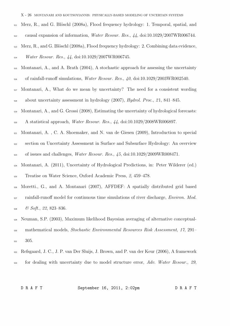
In detail the simulation procedure is carried out through the following steps:218

1. A parameter vector for the hydrological model is picked up at random from the219

model parameter space according to the probability distribution fε(ε).220

2. An input data vector for the hydrological model is picked up at random from the221

input data space according to the probability distribution fI(I).222

3. The hydrological model is run and a model prediction (or a vector of individual223

predictions) S(ε, I) is computed.224

4. A number n of realizations of the global model error (or vectors of individual errors)225

is picked up at random from the model error space according to the probability distribution226

fe|ε,I(e) and added to the model prediction S(ε, I).227



5. The simulation described by items from 1 to 4 is repeated j times. Therefore one228

obtains n · j (vectors of) realizations of the true variable to be predicted Qp.229

6. Finally the probability distribution fQp (Qp) is inferred through the realizations men-230

tioned in item 5.231

It is important to note that j needs to be sufficiently large, in order to accurately232

estimate the probability density fQp(Qp). It is also clarified that in a typical Monte Carlo233

procedure one would use n = 1 (where, to each simulation a different realisation of model234

error e would be generated). However, a larger n value multiplies the number of simulated235

points by a factor n with negligible increase of computer time (as the same hydrological236

simulation run is used for all n). We believe that a modest value of n (see application in237

Section 8) results in a good compromise of accuracy and computational efficiency. Figure238

1 shows a flowchart of the whole simulation procedure.239

Once the probability distribution of the true value to be predicted Qp is known the240

problems of hydrological modeling and uncertainty assessment are both solved.241

5. Discussion of the Underlying Assumptions

Like any scientific method, the blueprint proposed in Section 3 and 4 is based on as-242

sumptions in order to ensure applicability. When dealing with uncertainty assessment in243

hydrology, assumptions are often treated with suspect, because it is felt that they un-244

dermine the effectiveness of the method and therefore its efficiency and credibility with245

respect to users. We must admit, though, that assumptions are unavoidably needed to set246

up models, calibrate their parameters and estimate their reliability, whatever approach is247

used. Evidently, flawed assumptions may falsify statistical inference as well as any alterna-248

tive model of uncertain and deterministic systems. Therefore the target of the researcher249



should not be to avoid assumptions, but rather discuss them transparently, evaluate their250

effects and, when possible, check them, for instance through statistical testing.251

In order to discuss the assumptions conditioning the blueprint we introduced above,252

first note that the theoretical scheme is very general. In fact, we only assumed that model253

input data and parameters are random vectors which are independent to each other. Such254

assumption implies that parameter uncertainty is independent of data uncertainty and its255

influence on the results depends on data uncertainty itself. Unless this latter is very sig-256

nificant, we believe the assumption is reasonable. In principle the above assumption could257

be removed by estimating the joint probability distribution of input data and parameters258

and then picking up from this distribution the random outcomes at steps 1 and 2 of the259

simulation procedure described in Section 4. Actually, statistical inference of joint prob-260

ability distributions of model input data and parameters is likely to be affected by much261

uncertainty and therefore it may be more difficult to implement. We plan to study this262

solution in future research.263

One may note that further assumptions might be needed to estimate the probability264

distribution fe of model error, which might be non-Gaussian and affected by heteroscedas-265

ticity. For instance, in the application presented in Section 8 the meta-Gaussian approach266

by Montanari and Brath [2004] is applied. Actually, this method assumes that the joint267

probability distribution of model error and model simulation is stationary and independent268

of input uncertainty and parameter uncertainty, but the marginal probability distribution269

of the model error can eventually result heteroscedastic (see Section 8 and Montanari and270

Brath [2004]). If one used the Generalised Likelihood Uncertainty Estimation (GLUE;271

see Beven and Binley [1992]) different assumptions would be introduced depending on272



the (possibly informal) likelihood measure that is used to characterise the reliability of273

model output. No matter which method is used, any additional assumption introduced274

for inferring fe should be appropriately checked.275

A relevant issue has been pointed out by some authors (see, for instance, Beven et al.276

[2011]) who are convinced that epistemic errors arising from hydrological models might277

be affected by non-stationarity and therefore difficult (or impossible) to model by using278

statistical approaches. In our opinion epistemic uncertainty in itself, which is not chang-279

ing in time, cannot induce non-stationarity, which might instead be necessary to enrol280

when environmental changes are present. However, independently from its origin, non-281

stationarity can be efficiently dealt with by using non-stationary stochastic processes, by282

introducing and checking suitable assumptions.283

The conclusion of the above discussion can be summarised by saying that (a) the only284

relevant assumption conditioning the proposed blueprint is justified as long as data un-285

certainty is not very significant (see also additional discussion about this in Section 8.3).286

Within this respect, we would like to emphasise our opinion that in the presence of signifi-287

cant input data errors (also called “observation uncertainty”) any uncertainty assessment288

method is ill-posed and likely to end up with underestimation. Moreover, (b) the above289

assumption can in principle be removed although it is likely that this option turns out290

to be more difficult to handle in practice. And finally, (c) further assumptions might be291

needed for ensuring the practical application of the approach, which should be appropri-292

ately checked.293



6. Open Research Questions

The above discourse shows that to include a deterministic model within a stochastic294

framework is in principle possible. Although we explicitly focused on physically-based295

approaches, the blueprint that we are proposing is applicable to any deterministic scheme,296

therefore including conceptual and black-box models. We believe that incorporation of297

physically-based deterministic models bears a greater added value of the blueprint we are298

proposing. In fact, analyzing the randomness of physically-based systems is an invaluable299

opportunity to improve their understanding therefore increasing predictability, according300

to the “models of everywhere” concept [Beven, 2007].301

However, relevant research challenges and practical problems may prevent a successful302

application of the blueprint. First of all, numerical integration (e.g. the Monte Carlo303

simulation outlined in Section 4) is computationally intensive and may result prohibitive304

for spatially-distributed models. Therefore efficient simulation schemes are necessary,305

while too detailed spatial representations may not make any difference except in wasting306

computer time.307

Second, a relevant issue is the estimation of global model uncertainty, namely, the308

estimation of the probability distribution fe (e) of the model error. The literature has309

proposed a variety of different approaches, like the above mentioned GLUE method [Beven310

and Binley , 1992], the meta-Gaussian model [Montanari and Brath, 2004; Montanari and311

Grossi , 2008], Bayesian Model Averaging (BMA, Neuman [2003]) and BATEA [Kuczera312

et al., 2006]. However, the above methods rely on limiting assumptions and some of313

them are too computer intensive. We believe that estimating global model uncertainty in314

hydrology [Montanari , 2011] is still an open problem for which more focused research is315



needed. The proposed framework may facilitate streamlining of this research and linking316

it with other components within an holistic modeling approach.317

Finally, estimation of parameter uncertainty is a relevant challenge as well. Possibilities318

are the GLUE method [Beven and Binley , 1992] and the DREAM algorithm [Vrugt et al.,319

2007], which nevertheless are computer intensive as well and may turn out to be inpractical320

with spatially-distributed models applied to fine time scale at large catchments.321

7. Placing Uncertainty Assessment Techniques Within the Proposed

Blueprint

The blueprint proposed in Section 3 and 4 aims to provide a general theoretical frame-322

work for uncertainty assessment in hydrology. Indeed, the most frequently used techniques323

can be easily placed within it. For instance, the well known GLUE method [Beven and324

Binley , 1992] anticipated many of the concepts we are highlighting here, and in particular325

the idea of estimating uncertainty by turning from one to many applications of the hydro-326

logical model. In detail, the simulation procedure used within the classical applications327

of GLUE is much similar to what is presented in Section 4. The only relevant differ-328

ence is related to the estimation of global model error, which is resolved within GLUE329

by estimating the model likelihood, and therefore the probability distribution of the true330

variable to be predicted, through an integral performance measure or by fixing limits of331

acceptability [Liu et al., 2009; Winsemius et al., 2009]. In fact, likelihood is estimated332

within classical GLUE by adopting an informal approach, basing on a dummy likelihood333

measure (like the Nash-Sutcliffe efficiency in many GLUE applications). Basing on the334

blueprint proposed here, GLUE can then be defined as a statistical approach where model335

likelihood is estimated informally.336



Moreover, the proposed blueprint reduces to the meta-Gaussian approach by Montanari337

and Brath [2004], once that parameter uncertainty and input uncertainty are neglected.338

A similar reasoning applies to the Bayesian Forecasting System by Krzysztofowicz [2002],339

where parameter uncertainty is neglected and the probability distribution of the true340

variable to be predicted is estimated by inferring the joint probability distribution of true341

value and corresponding model output.342

8. An Example of Application

In order to illustrate the proposed blueprint with a practical example, an application is343

presented here below that refers to a rainfall-runoff model applied to a catchment located344

in Italy.345

8.1. The study catchment

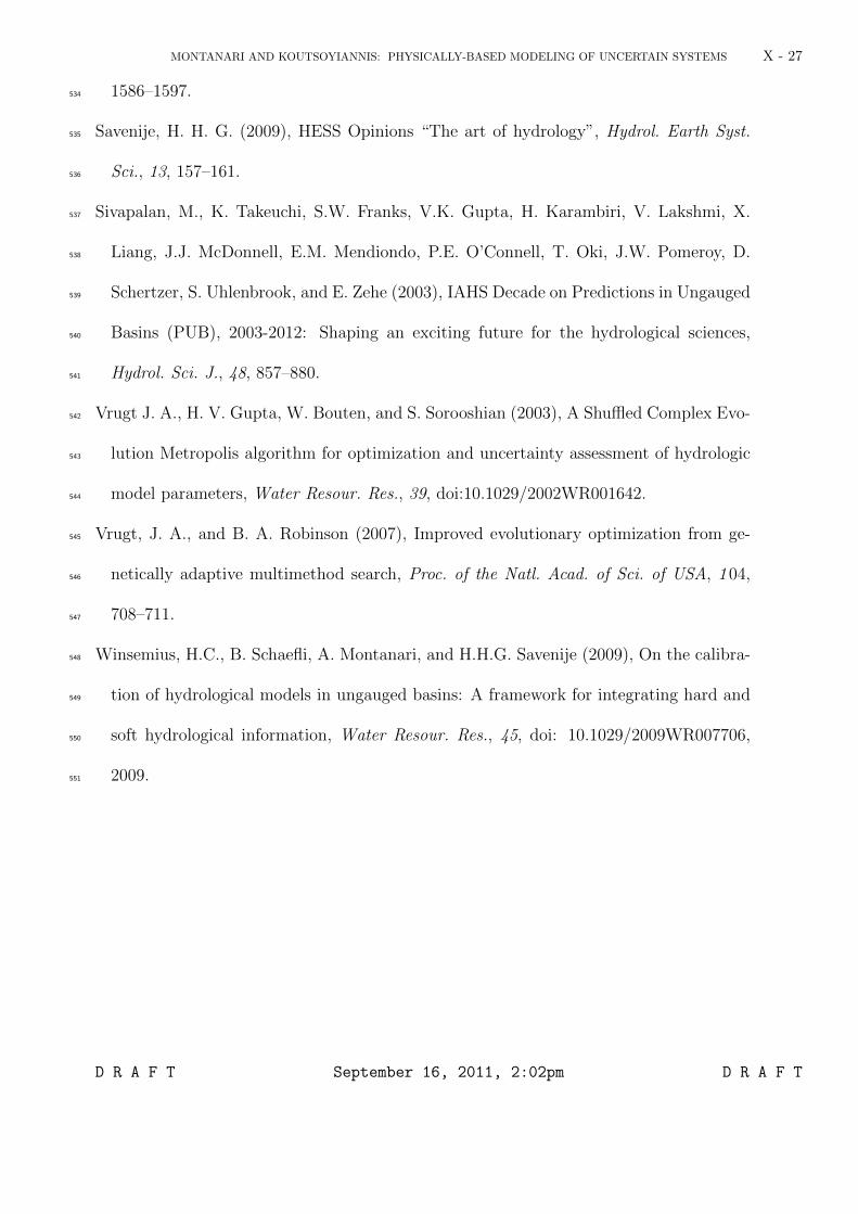
The application refers to the Leo River at Fanano, in the Emilia-Romagna region, in346

Northern Italy. Figure 2 shows the location of the catchment. The catchment area is347

64.4 km2 and the main stream length is about 10 km. The maximum elevation in the348

catchment is the Mount Cimone (2165 m a.s.l.), which is the highest peak in the northern349

part of the Apennine Mountains. The climate over the region is continental.350

Daily river flow data at Fanano are available for the period January 1st, 2003 - October351

26th, 2008, for a total of 2126 observations. For the same period, daily mean areal352

rainfall and temperature data over the catchment are available, as estimated by the Italian353

National Hydrographic Service basing on observation collected in nearby gauging stations.354

The observations collected from January 1st 2003 to December 31st 2007 were used355

for calibrating the rainfall-runoff model, while the period September 1st 2007 - October356



26th 2008 was reserved for its validation. We estimated the probability distribution of357

the model error by referring to the first year of the validation period (2007), in order358

to obtain a reliable assessment of fe|ε,I (e|ε, I) in a real world application. Note that the359

general formulation of eq. (8) is used, thereby accounting for heteroscedasticity in the360

model error itself. Finally, the period January 1st 2008 - October 26th 2008 was reserved361

for testing, in full validation mode, the proposed blueprint (rainfall-runoff modeling and362

uncertainty assessment).363

8.2. The rainfall-runoff model

The rainfall-runoff model is AFFDEF [Moretti and Montanari , 2007], a spatially-364

distributed grid-based approach where hydrological processes are described with365

physically-based and conceptual equations. In order to limit the computational require-366

ments, and in view of the limited catchment area, the Leo river basin was described367

by using only one grid cell, therefore applying a lumped representation. AFFDEF was368

calibrated by using DREAM [Vrugt et al., 2007], that is, a modified SCEM-UA global369

optimisation algorithm [Vrugt et al., 2003]. The DREAM method makes use of popula-370

tion evolution like a genetic algorithm together with a selection rule to assess whether a371

candidate parameter set is to be retained. The sample of retained sets after convergence372

can be used to infer the probability distribution of model parameters. Herein, a number373

of 1000 parameter sets were retained, which indirectly determine the density function374

fε (ε) of the parameter vector in a non-parametric empirical manner, fully respecting the375

dependencies between different parameters.376

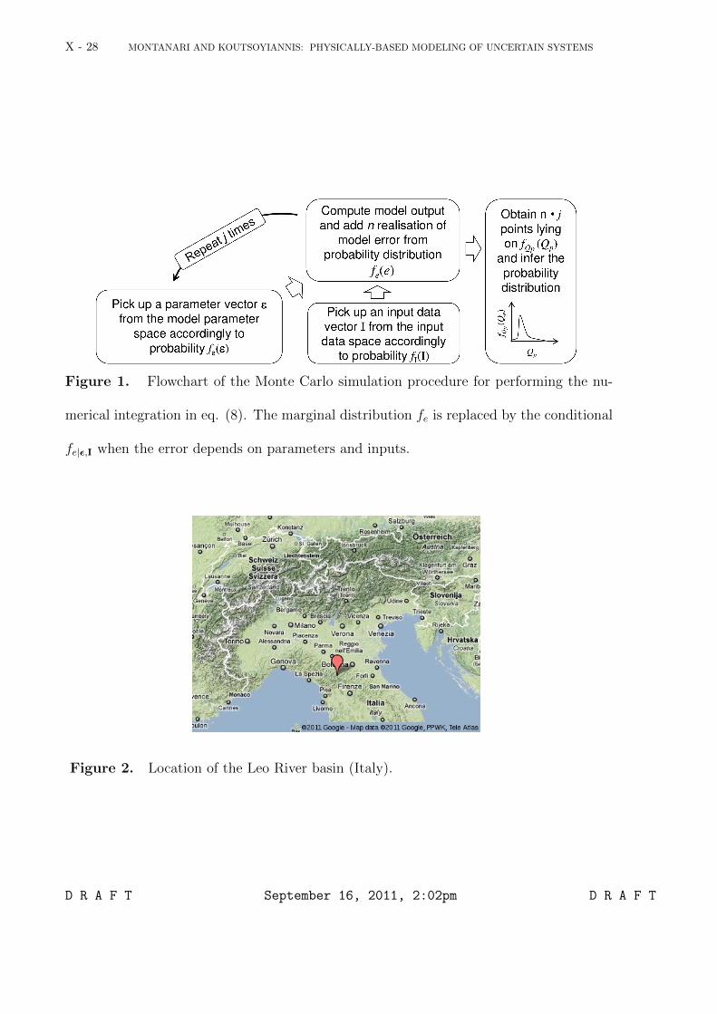
AFFDEF explained about 57% and 50% of the river flow variance in calibration and377

validation, respectively. Figure 3 reports a comparison during the validation period (2007378



and 2008) between observed and simulated hydrographs. This latter was obtained by using379

the best parameter set according to explained variance during the calibration period. One380

can see that a significant uncertainty affects the model performances, which is unlikely381

merely due to lumping the model at catchment scale. We are interested in checking382

whether the proposed blueprint provides a consistent assessment of such uncertainty.383

Finally, the probability distribution of the model error was inferred by using the meta-384

Gaussian approach by Montanari and Brath [2004]. In brief, the method recognizes that385

the error is affected by heteroscedasticiticy by accounting for the dependence of its condi-386

tional probability distribution on model prediction. In this way change of the statistical387

properties during time is efficiently modeled. The estimation of the joint probability dis-388

tribution of model simulation (provided by AFFDEF by using the best parameter set389

in terms of explained variance during the calibration period) and error is carried out390

by preliminarily transforming the data to the Gaussian probability distribution. In the391

Gaussian domain a bivariate Gaussian distribution is finally estimated. The goodness-392

of-fit provided by the meta-Gaussian approach was checked by using the statistical tests393

described in Montanari and Brath [2004], where more details on the procedure can be394

found.395

8.3. The simulation procedure

We assumed to neglect input data uncertainty because no information was available396

to infer the probability distribution of the available observations. This is an important397

limitation in many practical applications. In particular, input uncertainty is usually398

dominant in real time flash-flood forecasting, where input rainfall to a rainfall-runoff399

model is usually predicted to increase the lead time of the river flow forecasting. If a400



probabilistic prediction for rainfall is available then input uncertainty can be efficiently401

taken into account in the blueprint proposed above. In alternative, input uncertainty can402

be estimated by using expert knowledge or Bayesian procedures like BATEA [Kuczera et403

al., 2006]. Given that the present application refers to a past period and excludes future404

forecast inputs, and since data series have been tested, it is reasonable to assume data405

certainty, with the awareness that we may slightly underestimate prediction uncertainty406

in this case.407

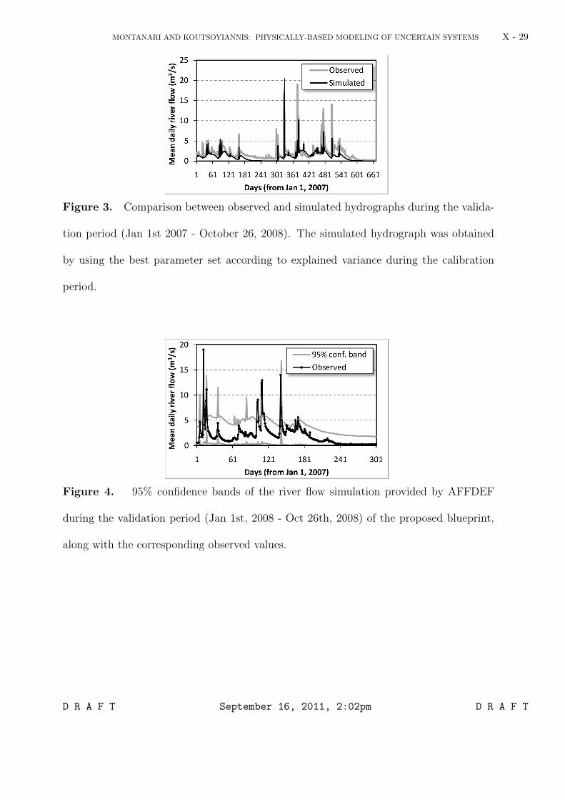
The simulation procedure was performed by running AFFDEF during the 300-day val-408

idation period January 1st 2008 - October 26, 2008, for each of the j = 1000 parameter409

sets retained by DREAM. Then, n = 100 random outcomes from the probability distribu-410

tion of the model error were added to each observation of the 1000 simulated data series,411

therefore obtaining 1000 · 100 simulations of the data value referred to each of the above412

300 days, which allowed us to estimate the related probability distribution. The above413

j and n values were selected by estimating the number of sampling points to efficiently414

infer the shape of the related probability distributions.415

Figure 4 shows the 95% confidence band of the model simulation, along with the corre-416

sponding observations. It can be seen that the results are physically meaningful and, in417

our opinion, confirm the efficiency of the proposed blueprint. In fact, the confidence bands418

are quite large as one would expect by looking at the performances of the model, which419

underline the presence of significant uncertainty. A number of data points are located420

outside the confidence bands as one would expect by considering that the band itself is421

drawn at the 95% confidence level.422



9. Conclusions

A new blueprint is presented for formulating physically-based models of uncertain hy-423

drological systems, which in effect means all hydrological systems. The main advantages424

of the proposed methodological scheme are that (a) hydrological modeling and uncertainty425

assessment are jointly carried out and (b) a general theoretical framework is elaborated426

for uncertainty estimation in hydrology, which includes as special cases the existing and427

most frequently used methods.428

Basically, the blueprint proposes to incorporate deterministic hydrological models within429

a stochastic framework. This solution is suggested by our convincement that probability430

is the most efficient and objective technique for uncertainty assessment. Shifting from the431

deterministic to the stochastic formulation requires passing from one to many applications432

of the hydrological model. What we suggest is not new in practical applications and con-433

stitutes also the rationale underlying some of the existing uncertainty assessment methods434

like GLUE [Beven and Binley , 1992]. However, a comprehensive theoretical framework435

is proposed, along with a detailed discussion of the underlying assumptions, therefore436

allowing one to structure in a objective setting the application of hydrological models in437

order for uncertainty to be taken into account and estimated.438

An application to an Italian river basin is presented for illustrating the introduced439

blueprint. Although a simplifying assumption was introduced to neglect data uncertainty440

and a lumped rainfall-runoff model was used, the case study shows that the proposed441

approach is efficient and physically meaningful.442

We believe the theoretical framework introduced here may open new perspectives re-443

garding modeling of uncertain hydrological systems. In fact, statistical analysis of un-444



certainty and predictability offers valuable indications to improve our understanding of445

real systems and better understand their (possibly) changing or shifting behaviors and446

their reaction to (human induced) changes. Last but not least, we believe that the pro-447

posed procedure is very useful for educational purposes, putting the basis for developing448

a unified theoretical basis for uncertainty assessment in hydrology.449

Relevant research questions are still open. The proposed procedure is based on run-450

ning multiple simulations and therefore it is computationally intensive. For this reason,451

application to very detailed spatial representation implemented on complex systems may452

require significant computational resources. Finally, estimation of parameter uncertainty,453

global model uncertainty and data uncertainty may represent relevant problems for some454

real world applications, for which additional and focused research is needed.455

Acknowledgments. To authors are grateful to Francesco Laio, Keith Beven and Elena456

Montosi for providing very useful comments and help. A.M. was partially supported by457

the Italian government through the grant “Uncertainty estimation for precipitation and458

river discharge data. Effects on water resources planning and flood risk management”.459

References

Abbot, M. B., J. C. Bathurst, J. A. Cunge, P. E. O’Connell, and J. Rasmussen (1986),460

An introduction to the European Hydrological System - Systme Hydrologique Europen,461

SHE. 2. Structure of a physically-based, distributed modeling system., J. Hydrol., 102,462

87–77.463

Beven, K. J. (1989), Changing ideas in hydrology The case of physically-based models,464

J. Hydrol., 105, 157–172.465



Beven, K. J., and A. M. and Binley (1992), The future of distributed models: Model466

calibration and uncertainty prediction, Hydrol. Proc., 6, 279–298.467

Beven, K. J. (2001), How far can we go in distributed hydrological modeling, Hydrol. and468

Earth System Sci., 5, 1–12.469

Beven, K. J. (2002), Towards an alternative blueprint for a physically based digitally470

simulated hydrologic response modeling system, Hydrol. Proc., 16, 189–206.471

Beven, K. J. (2006), A manifesto for the equifinality thesis, J. Hydrol., 320, 18–36.472

Beven, K. J. (2007), Towards integrated environmental models of everywhere: uncertainty,473

data and modelling as a learning process, Hydrol. and Earth System Sci., 11, 460–467.474

Beven, K. J., P. J. Smith, and A. Wood (2011), On the colour and spin of epistemic error475

(and what we might do about it), Hydrol. Earth Syst. Sci. Discuss., 8, 5355–5386.476

Box, G. E. P., and G. C. Tiao (1973), Bayesian Inference in Statistical Analysis, Addis-477

onWesley, Boston, Massachusetts.478

Di Baldassarre, G, and A. Montanari (2009), Uncertainty in river discharge observations:479

A quantitative analysis. Hydrol. and Earth Sys. Sci., 13, 913–921.480

Freeze, R. A., and R. L. Harlan (2008), Blueprint for a physically-based, digitally- simu-481

lated hydrologic response model, J. Hydrol., 9, 237–258.482

Grayson, R. B., I. D. Moore, and T. A. McMahon, (1992), Physically-based hydrologic483

modeling. 2. Is the concept realistic?, Water Resour. Res., 28, 2659–2666.484

Hopp, L., C. Harman, S. L. E. Desilets, C. B. Graham, J. J. McDonnell, and P. A.485

Troch (2009), Hillslope hydrology under glass: confronting fundamental questions of486

soil-water-biota co-evolution at Biosphere 2, Hydrol. Earth Syst. Sci., 13, 2105-2118.487



Kundzewicz, Z. W. (2007), Predictions in Ungauged Basins: PUB Kick-off, Proceedings488

of the PUB Kick-off meeting held in Brasilia, 2022 November 2002, IAHS Publ. 309,489

38–44.490

Koutsoyiannis, D., C. Makropoulos, A. Langousis, S. Baki, A. Efstratiadis, A.491

Christofides, G. Karavokiros, and N. Mamassis (2009), HESS Opinions: “Climate, hy-492

drology, energy, water: recognizing uncertainty and seeking sustainability”, Hydrol.493

Earth Syst. Sci., 13, 247–257.494

Koutsoyiannis, D. (2010), HESS Opinions “A random walk on water”, Hydrol. Earth Syst.495

Sci., 14, 585–601.496

Koutsoyiannis, D. (2011), Hurst-Kolmogorov dynamics and uncertainty, Journal of the497

American Water Resources Association, 47, 481–495.498

Krzysztofowicz, R. (2002), Bayesian system for probabilistic river stage forecasting, J. of499

Hydrol., 268, 16–40.500

Kuczera, G., D. Kavetski, S. Franks, and M. Thyer (2006), Towards a Bayesian total501

error analysis of conceptual rainfall-runoff models: Characterising model error using502

storm-dependent parameters, J. Hydrol., 331, 161–177.503

Laio, F. (2006), A vertically extended stochastic model of soil moisture in the root zone,504

Water Resour. Res., 42, doi:10.1029/2005WR004502.505

Lasota, D. A., and M. C. Mackey (1985), Probabilistic properties of deterministic systems,506

Cambridge University Press.507

Liu Y, J. Freer, K. J. Beven, and P. Matgen (2009), Towards a limits of acceptability508

approach to the calibration of hydrological models: Extending observation error, J. of509

Hydrol., 367, 93–103.510



Merz, R., and G. Bloschl (2008a), Flood frequency hydrology: 1. Temporal, spatial, and511

causal expansion of information, Water Resour. Res., 44, doi:10.1029/2007WR006744.512

Merz, R., and G. Bloschl (2008a), Flood frequency hydrology: 2. Combining data evidence,513

Water Resour. Res., 44, doi:10.1029/2007WR006745.514

Montanari, A., and A. Brath (2004), A stochastic approach for assessing the uncertainty515

of rainfall-runoff simulations, Water Resour. Res., 40, doi:10.1029/2003WR002540.516

Montanari, A., What do we mean by uncertainty? The need for a consistent wording517

about uncertainty assessment in hydrology (2007), Hydrol. Proc., 21, 841–845.518

Montanari, A., and G. Grossi (2008), Estimating the uncertainty of hydrological forecasts:519

A statistical approach, Water Resour. Res., 44, doi:10.1029/2008WR006897.520

Montanari, A. , C. A. Shoemaker, and N. van de Giesen (2009), Introduction to special521

section on Uncertainty Assessment in Surface and Subsurface Hydrology: An overview522

of issues and challenges, Water Resour. Res., 45, doi:10.1029/2009WR008471.523

Montanari, A. (2011), Uncertainty of Hydrological Predictions, in: Peter Wilderer (ed.)524

Treatise on Water Science, Oxford Academic Press, 2, 459–478.525

Moretti., G., and A. Montanari (2007), AFFDEF: A spatially distributed grid based526

rainfall-runoff model for continuous time simulations of river discharge, Environ. Mod.527

& Soft., 22, 823–836.528

Neuman, S.P. (2003), Maximum likelihood Bayesian averaging of alternative conceptual-529

mathematical models, Stochastic Environmental Resources Risk Assessment, 17, 291–530

305.531

Refsgaard, J. C., J. P. van Der Sluijs, J. Brown, and P. van der Keur (2006), A framework532

for dealing with uncertainty due to model structure error, Adv. Water Resour., 29,533



1586–1597.534

Savenije, H. H. G. (2009), HESS Opinions “The art of hydrology”, Hydrol. Earth Syst.535

Sci., 13, 157–161.536

Sivapalan, M., K. Takeuchi, S.W. Franks, V.K. Gupta, H. Karambiri, V. Lakshmi, X.537

Liang, J.J. McDonnell, E.M. Mendiondo, P.E. O’Connell, T. Oki, J.W. Pomeroy, D.538

Schertzer, S. Uhlenbrook, and E. Zehe (2003), IAHS Decade on Predictions in Ungauged539

Basins (PUB), 2003-2012: Shaping an exciting future for the hydrological sciences,540

Hydrol. Sci. J., 48, 857–880.541

Vrugt J. A., H. V. Gupta, W. Bouten, and S. Sorooshian (2003), A Shuffled Complex Evo-542

lution Metropolis algorithm for optimization and uncertainty assessment of hydrologic543

model parameters, Water Resour. Res., 39, doi:10.1029/2002WR001642.544

Vrugt, J. A., and B. A. Robinson (2007), Improved evolutionary optimization from ge-545

netically adaptive multimethod search, Proc. of the Natl. Acad. of Sci. of USA, 104,546

708–711.547

Winsemius, H.C., B. Schaefli, A. Montanari, and H.H.G. Savenije (2009), On the calibra-548

tion of hydrological models in ungauged basins: A framework for integrating hard and549

soft hydrological information, Water Resour. Res., 45, doi: 10.1029/2009WR007706,550

2009.551



Figure 1. Flowchart of the Monte Carlo simulation procedure for performing the nu-

merical integration in eq. (8). The marginal distribution fe is replaced by the conditional

fe|ε,I when the error depends on parameters and inputs.

Figure 2. Location of the Leo River basin (Italy).



Figure 3. Comparison between observed and simulated hydrographs during the valida-

tion period (Jan 1st 2007 - October 26, 2008). The simulated hydrograph was obtained

by using the best parameter set according to explained variance during the calibration

period.

Figure 4. 95% confidence bands of the river flow simulation provided by AFFDEF

during the validation period (Jan 1st, 2008 - Oct 26th, 2008) of the proposed blueprint,

along with the corresponding observed values.


A Blueprint for Physically-Based Modeling of Uncertain ... · 36 Given that traditionally...

Documents

Transcript of A Blueprint for Physically-Based Modeling of Uncertain ... · 36 Given that traditionally...