A Blocking Gibbs Sampling Method to Detect Major

Genes with Phenotypic Data from A Diallel Mating

Wen Zeng1, Sujit Ghosh1 and Bailian Li2

1Department of Statistics, 2Department of Forestry, Box 8002, North Carolina State

University, Raleigh, NC 27695-8002, USA.

Institute of Statistics Mimeo Series# 2560

1

SUMMARY: Diallel mating is a frequently used design for estimating the additive and

dominance genetic (polygenic) effects involved in quantitative traits observed in the half- and

full-sib progenies generated in plant breeding programs. Gibbs sampling has been used for

making statistical inferences for a mixed inheritance model (MIM) that includes both major

genes and polygenes. However, using this approach, it has not been possible to incorporate

the genetic properties of major genes with the additive and dominance polygenic effects in a

diallel mating population. A parent block Gibbs sampling method was developed in this study

to make statistical inferences about the major gene and polygenic effects on quantitative traits

for progenies derived from a half-diallel mating design. Using simulated data sets with

different major and polygenic effects, the proposed method accurately estimated the major

and polygenic effects of quantitative traits, and possible genotypes of parents and progenies.

The impact of specifying different prior distributions was examined and was found to have

little effect on inference on the posterior distribution. This approach was applied to one

experimental data of Loblolly pine (Pinus taeda L.) derived from a 6-parent half-diallel

mating. The result suggested that there might be a recessive major gene affecting height

growth in this diallel population.

Key words: Bayesian method; Polygenic effects, Diallel mating design; Markov Chain

Monte Carlo (MCMC); Mixed inheritance model (MIM); Quantitative trait.

2

1. Introduction

Quantitative genetics has contributed significantly to the improvement of productivity and

quality in animal and plant breeding programs. In the classic quantitative method, traits are

assumed to be controlled by polygenes, i.e., many genes, with each gene having a small effect

on a quantitative trait. With advances in molecular technology and computational statistics,

there is strong evidence that some quantitative traits may be controlled by a number of genes

that have relatively large effects on phenotype. For example, major genes or quantitative trait

loci (QTL) have been found in Drosophilae (Long et al., 1995), domestic animals (Piper and

Shrimpton, 1989), rice (Jiang et al., 1994) and tree species (Wilcox et al., 1996; Kaya et al.,

1999, Remington and O’Malley, 2000). A mixed-inheritance model (MIM) that includes a

major gene together with polygenes, instead of strictly polygenes, has been developed

recently for analyzing some quantitative traits (Elston and Stewart, 1971; Kinghorn et al.,

1994; Janss et al., 1997; Zeng and Li, 2003).

Several statistical approaches have been developed for the detection of major genes

for quantitative traits, based on phenotypic data. Methods based on analysis of variance have

been used to infer the number of major loci contributing to growth variation of interspecific

aspen hybrids (Li and Wu, 1996; Wu and Li, 1999; Wu and Li, 2000). Several statistical

methods using simple non-parametric tests for departure from normality have been used for

detecting major gene segregation, but not for estimating major gene effects (Mérat, 1968;

Fain, 1978; Karlin and Williams, 1981; Lynch and Walsh, 1998; Zeng and Li, 2003). Other

approaches based on maximum likelihood and Bayesian inference have been developed for

the MIM to detect major genes affecting quantitative traits in animal (Hoeschele, 1988; Knott

et al., 1991; Janss et al., 1997; Lund and Jensen, 1999), crop (Wang et al., 2001) and tree

3

species (Wu et al., 2001). Most of these methods are based on either a multiple-generation

pedigree, or else a progeny population derived from either a nested mating design (in the case

of animal breeding) or a factorial mating design (in the case of tree hybrids). To our

knowledge, however, no statistical methods have been developed for a progeny population

derived from a diallel mating design.

Diallel mating is one of the most commonly used designs in plant and tree breeding

programs (Hallauer and Miranda, 1981; Zobel and Talbert, 1984). Unlike factorial mating,

where male parents from one group are crossed with females from a second group, parents in

a diallel design are crossed either as male or female with other parents in a single group

(Griffing, 1956). A half-diallel mating is the diallel mating without self and reciprocal

crosses where both half-sib and full-sib progenies are produced for each of six parents. Diallel

mating yields two levels of polygenic effects, i.e., the general combining ability (GCA) of

parents due to additive polygenic effects, and the specific combining ability (SCA) of crosses

due to dominant polygenic effects. The unique feature of diallel mating, the model for an

observation having two main effects, has made it difficult to analyze with standard statistical

programs for even polygenetic effects (Xiang and Li, 2001). Thus, it has been difficult to

incorporate genetic properties of major genes with the two levels of polygenic effects in a

MIM model for analyzing diallel data. Because of high-dimensional marginalization of the

joint density over the unknown single genotype and polygenic effects, it is practically

impossible to maximize the likelihood function associated with such a model using analytical

and/or numerical techniques (Le Roy et al., 1989; Knott et al., 1991). For animal breeding,

the Gibbs sampling algorithm has been found to be reasonably effective in making inference

for a mixed inheritance model in a nested mating design, in which parents can be either male

4

or female, but not both (Janss et al., 1997). Such analyses were primarily based on the half-

sib relationships of parents (male or female) and their progenies. In the case of tree-breeding

programs, diallel progenies are usually planted at several locations or site types to determine

their growth potential under different environments. The potentially large environmental

variation, as well as genotype by environmental interaction, relative to animal breeding, may

affect the statistical power for major gene detection (McKeand et al., 1997). Although the

Bayesian approach may have potential for major gene detection, its usefulness for MIM

analysis of diallel data is unknown, because of the two types of polygenic effects and the

heterogeneous environmental variance. It is important to evaluate the ability of the Bayesian

approach for detecting the segregation of major genes with a diallel progeny population

across environments.

In this study, we developed a Bayesian approach, using a parent blocking Gibbs

sampling, to make inferences about major genes and polygenic effects (GCA and SCA) that

control quantitative traits for a progeny population derived from a half-diallel mating design

without self and reciprocal crossings. Computer simulations were done to examine the effects

of different prior distributions and design matrix, either full-ranked or non-full-ranked, on the

proposed statistical method. A case study with one half-diallel progeny population of Loblolly

pine (Pinus taeda L.) was used to detect a major gene for height growth and to illustrate the

application of the method.

2. The Mixed Inheritance Model

A mixed inheritance model (MIM) is adopted in this study for the diallel analysis, in which

phenotypes are assumed to be influenced by a single major gene and the polygenic effects. A

5

half-diallel mating design, with parents selected from a base population under Hardy-

Weinberg and linkage equilibrium (Falconer and Mackay, 1996), and full-

sib families, is used to study the MIM. Each full-sib family is tested at several sites,

following a randomized complete block design with several trees per full-sib family within

each block, and several blocks within each site. The statistical model for a MIM can be

written as a mixed linear model:

pn

spp nnn =− 2/)1(

eWLmZuXµY +++= (1)

The notation definitions are listed in Table 1. Unlike MIM for an animal population,

there is no incidence matrix in the major gene effect term, because data are only the

phenotypic observations of progenies in a tree population, rather than progenies plus parents

(sires and dams) as in an animal population. By assuming for e and giving

location and scale parameters, the vector of data is also normally distributed as:

Z Y

),( 2I0N eσ

Y

),~, 22 IWLmZuN(XµmW,u,µ,|Y ee σσ ++

The single major gene under the traditional genetic model of one gene with two alleles

(Falconer and Mackay, 1996) is assumed to be a bi-allelic ( and ), autosomal locus with

Mendelian transmission probabilities, such that each progeny has one of the three possible

genotypes: , and with genetic effects and

1A 2A

11 AA 21A A 22 AA ,, da a− respectively. For progeny

, the genotype is represented as a random vector , with values (1,0,0), (0,1,0),

or (0,0,1) corresponding to the three possible genotypes of , , and

respectively. Given the two parent genotypes and , the genotype distribution of

progeny is denoted as . This distribution describes the probability of

),...,1( nkk = kw

11 AA 21 AA 22 AA

)(1 kpw )(2 kpw

k ),|( )(2)(1 kpkpkp www

6

alleles constituting genotype being transmitted from parents with genotypes and

when segregation of allele follows Mendelian transmission probabilities. Because of

the conditionally independent structure of the genotypes, the joint genotype distribution of

progenies can be written as:

kw )(1 kpw

)(2 kpw

(2) ),|(p)( )(2)(11

kpkpk

n

kpp wwww|W ∏

=

=

where are the genotypes of parents. The parent genotypes are sampled from a base

population with genotypes in Hardy-Weinberg equilibrium (Falconer and Mackay, 1996).

This is a reasonable assumption for tree breeding populations because individual trees serving

as parents are usually selected randomly from natural populations. Given the favorable allele

frequency in the base population

pw pn

)( 1Apf = , the probability distribution of the genotype of

parent i is assumed to be which follows Hardy-Weinberg proportions. Because of

the independence among parents, the joint genotype distribution of parents can be written as:

)|( fp piw

(3) )|()|(1

fpfp pi

n

ip

p

ww ∏=

=

In order to fully specify the Bayesian model, normal priors are assigned to the overall

mean µ=µ , and major gene effects ),( da=′m , i.e. , and

, where , =1, 2 and 3 are the hyper-parameters of the prior distribution. In

the simulation and real data analysis we used k

),,0(~ Nµ 21k

3v

),0(~ 22kNa

),0(~ 23kNd 2

ik i

i =4, i=1,2,3. Variance components, , and

are assumed to arise independently from conjugate inverted gamma distributions (IG), i.e.

and where

2gσ 2

sσ

2eσ

),,(~ 112 vIGg γσ ),(~ 22

2 vIGs γσ ),,(~ 32 IGe γσ iγ and are hyper-parameters.

For our application, we used

iv

iγ =2, and iiiv σγ ˆ*)1( −= , =i 1, 2 and 3 for ,ˆˆ,ˆˆ 21 sg σσσσ ==

7

and , where eσσ ˆˆ 3 = iσ̂ are obtained from a preliminary study using frequency distribution

method. The conjugate Beta prior is used for the allele frequency, i.e., ),(~)( ffBetafp βα ,

where fα and fβ are prior distribution parameters. We have chosen 1== ff βα to express

prior ignorance.

The joint posterior density of all unknowns, given the data , is proportional to the

product of the likelihood function and the prior densities:

Y

)()|()|()()()()()()|()|()(),(

)|,,,,(222222

222

fpfppdpapppppppp

fp

ppsgsgee

esgp

wwWµsgWu,m,µ,|Y

YwW,u,m,µ,

σσσσσσ

σσσ ∝

∏∏

∑

∑

=

−−

=

+−

=

−

+−

=

−+−

−

−==×

⎭⎬⎫

⎩⎨⎧−

⎭⎬⎫

⎩⎨⎧−

⎭⎬⎫

⎩⎨⎧−×

⎭⎬⎫

⎩⎨⎧−

⎭⎬⎫

⎩⎨⎧−×

⎪⎭

⎪⎬⎫

⎪⎩

⎪⎨⎧−

⎪⎭

⎪⎬⎫

⎪⎩

⎪⎨⎧−

⎭⎬⎫

⎩⎨⎧−×

⎭⎬⎫

⎩⎨⎧

−−−′−−−−∝

gff

ss

gg

n

igpi

n

kkpkpgk

ss

n

jj

s

n

s

gg

n

ii

g

n

ge

e

e

n

e

fffpp

dk

akk

vs

vg

v

1

11

1)(2)(1

223

222

22

1

22)1(2

1

22

22

21)1(2

1

22

2223)1(2

222

)1()|(),|(

21exp

21exp

21exp

exp)(2

1exp)(

exp)(2

1exp)(exp)(

)()(2

1exp)(

2

13

βα

γ

γγ

µ

σσ

σσ

σσ

σσ

σσ

σσ

wwwwww

WLmZuXµyWLmZuXµy

(4)

In order to study the effects of the prior on the method’s behavior with this data

structure, improper flat priors are used for the overall meanµ , and major gene effect a

and , i.e., d ∝)(µp constant, ∝)(ap constant, and ∝)(dp constant, besides normal priors.

The prior for any is always inverted Gamma. 2σ

3. Gibbs sampling

3.1 Parent blocking

8

In order to make statistical inferences about unknowns, the marginal posterior distributions

for the model parameters are of interest. However, it appears to be almost impossible to

obtain such marginals for our model. In analytical approaches, the study of marginal

densities would require integration and/or summation. Often such marginalizations are not

feasible to compute or even express in closed form for a high-dimensional model like MIM,

as presented in equation (4). But this difficulty can be circumvented by means of simulation-

based methods. The Gibbs sampler is based on sampling random varieties from a Markov

chain (MC) with its stationary distribution as the posterior distribution, and the sampling from

the MC used to perform the high dimensional Monte Carlo integration (Gelfand and Smith,

1990; Brooks, 1998). Samples are obtained from the full conditional distributions, which form

the transition probabilities of the Markov chain. Each time a full conditional distribution is

visited, it is used to sample the corresponding parameter, while other parameters are

considered to be fixed, and then the realized value is substituted into the full conditional

distribution of all other parameters.

To improve the mixing and hence the speed of convergence, it is possible to sample

several parameters simultaneously, called a ‘block,’ from their joint conditional distribution

instead of updating all parameters univariately. As long as all parameters are updated, the new

Markov chain will still have equation (4) as the density of stationary distribution. Unlike an

animal population where data include parents and their offspring, and usually span several

generations, in a tree population we consider only the progeny observations in the data Y with

just two generations. The sire block strategy (Janss et al., 1997) has worked well for animal

populations. Since in a diallel mating design, one tree served as a male as well as a female, we

modified ‘a sire blocking’ into ‘a parent blocking’. In a parent blocking, the genotypes of a

Y

9

parent and its half-sib offspring are treated as a block and updated simultaneously.

Consequently, in each cycle, the genotype of every offspring is updated twice instead of once

a cycle as each offspring has two parents. Given the work of Liu et al. (1994), and Robert and

Sahu (1997), it seemed to us that the block Gibbs sampler would mix faster than the ordinary

one-at-a-time version that updates each component sequentially. Blocking is generally

effective when the elements within the block are highly correlated compared to the correlation

between blocks.

3.2 Full conditional distributions

Full conditional distributions are derived from the joint posterior distribution (4). For

notational convenience, the MIM can be rewritten as: eHθY += , where

is a ( ) matrix, and is a (

Z]:WL:[XH =

nxp ),,,(),( '' '''' s,gu,mµθ daµ== ),...,,( 21 pθθθ= p x1) parameter

vector.

In order to implement the ‘parent blocking,’ an exact calculation of the joint conditional

distribution of a parent and its all offspring is required. The joint conditional distribution for

parent is: , where denotes the

number of offspring of parent i , and the offspring are indexed by , or simply

, where . By definition, this distribution is proportional to

.

i ),,,,,,,|,...,,( 222)()()1( YθwWwww esgpiliniipi fp

iσσσ−− in

)(),...,2(),1( iniii

)(li inl ,...,1=

),,,,,,,|,...,(*),,2s,,,,,|( 222

)()()1(22

)( YθwWwwYθwWw esgpliniiegpilipi fpfpi

σσσσσσ −−−

The first term is the genotypic distribution of the parent i , marginalized with respect to the

genotypes of its offspring. The second term is the joint distribution of offspring genotypes

conditional on the parents’ genotypes. To calculate the genotype distribution of parent , the

three possible genotypes of all offspring must be summed after weighting each genotype by

i

10

its relative probability. The final marginalized full conditional distribution for the major

genotype of the parent is: i

∏∑∈ =

−−

====

∝=

)(

3

121

222)(

)|~(),|(*)|(

),,,,,,,|(

lik bbkkpTpbkTpi

esgpiliTpi

yppfp

fp

wwwwwwwww

YθwWww σσσ (5-1)

where uZ kkk yy −−= µ~ is called the adjusted record, are the kkZ th rows of the matrices

, and has the same notation as . The penetrance function (or weight) is: Z bw Tw

⎭⎬⎫

⎩⎨⎧

−−∝)= 22 )~(

21exp| Lmwww kk

ebk yp

σ~( ky . The probabilities here are given up to a

constant of proportionality and st be normalized to ensure that . ∑=

==3

11)(

TTpip ww

For the genotypes of offspring, the marginalized full conditional distributions are the

same as the usual full conditional distributions found by extracting from equation (4) the term

in which , is present. i.e. )(, likk ∈w

)|~(*),|(),,,,,,,|( )(2)(1222

TkkkpkpTkesgpkTk yppfp wwwwwwYθwWww ==∝= −− σσσ (5-2)

The full conditionals for allele frequency, location parameters and variance components

are obtained by just extracting the relevant terms from the joint posterior density in equation

(4) (for details see Zeng, 2000).

3.3 Updating scheme

The algorithm based on parent block updating is summarized as the following:

I. initiate , , and with some reasonable starting values; θwW ,, p2gσ 2

sσ 2eσ

11

II. sample major genotypes nkni kppi ,...,1,,,...,1, == ww from full conditional distributions,

(5-1) and (5-2), by parent blocking. The updating scheme is to

1) update parent 1 and its offspring, plus , in one block, with 1pw )(1 lpw [ ] [ ]tpn

tp p

ww ,...,2

known;

2) update parent 2 and its offspring, plus , in one block, with

known;

2pw )(2 lpw

[ ] [ ] [ ]tpn

tp

tp p

www ,...,, 31

1+

… …

) update parent and its offspring, plus , in one block with

known; each offspring updates twice in each cycle;

pn pnppnw )(lpnp

w

[ ] [ ]1)1(

11 ,..., +

−+ t

nptp p

ww

The parents may be updated in any order. In fact, it is possible to update in random order in

each iteration.

III. sample allele frequency , location parameters f θ , and variance components , and 2gσ 2

sσ

2eσ from the full conditional distribution;

IV. repeat II-III, these steps constituting one iteration.

4. Simulation

4.1 Data generation process

To evaluate the procedure with this data structure, simulated data with both major gene and

polygenic components were generated for this study. A 6-parent half-diallel mating design

with 4 test sites and 6 blocks per site is used to simulate phenotypic observations, although

the site effects and block within site effects are both set to zero. Six parents are chosen

randomly from a base population in which the major gene and polygenic parameters are

12

defined. There are 15 full-sib families, 6 progenies per family per block per test site, and a

total of 2160 progenies across 4 test sites.

For all progenies, phenotypic observations are simulated according to the model (1). The

polygenic effect ( ) include Zu SGG ++ 21 , where 1G and are GCA effects for 2 parents

with prior distribution , and is SCA effects with prior distribution . Two

genetic parameters, the narrow sense heritability of polygenic inheritance

(where is the total phenotypic variance), and the ratio of dominance to additive genetic

variance of polygenic inheritance, , are used to calibrate these polygenic

quantities (Huber et al., 1992).

2G

),0( 2gN σ S ),0( 2

sN σ

222 /4 pgh σσ=

2pσ

22 / gsr σσ=

The major genotypes of parents and progenies are simulated according to equation (3)

and (2). The major gene variance component is calculated as following:

[ ] [ ]22222 )1(2)21()1(2 dffadfffdam −++−−=+= σσσ . The total phenotypic variance is

. The relationship between polygenic effects and major gene

effects is assumed to be additive. For our simulation, the parameters are set to =0.2,

0.12 22222 =+++= esgmp σσσσσ

2h r =0.5,

=1.0, =0.0, and =0.2. The realized favorable allele frequency ( ) is 0.167. The major

genotypes of six parents are , , , , and . The effect of the

single gene in this case is to be detected and estimated.

a d f f

22 AA 22 AA 22 AA 21 AA 21 AA 22 AA

4.2 Effects of prior distribution, initial value, and design matrix

For the overall mean (µ ), the additive major gene effect ( a ) and the dominance major gene

effect ( ), the priors are chosen as a flat distribution, i.e., d )(),( app µ and , and are )(dp

13

proportional to a constant, or chosen as a normal distribution, i.e. )(),( app µ and , and

have , where

)(dp

),0( 2KN 4=K is used in the analysis. Both uniform and normal priors are used

in the model, respectively, to see the effect of priors on posterior inference.

The design matrix for the random polygenic effects (GCAs and SCAs) can be either full

rank by putting constraints , or singular. Both design matrices are used to

test its effect on the MCMC method, especially on the convergence of MCMC.

∑∑==

==sg n

jj

n

ii sg

11

0,0

Initial values of GCA, SCA and variance components, are obtained from the

traditional genetic model analysis (without major gene effect). These estimates are used as

initial values for the Markov chain. For the major gene, the ranges for , and are [0.0,

1.0], [0.0, 0.5], and [0.1, 0.5] respectively (Table 2). The genotypes of parents are generated

by , assuming that parents are all from a base population with Hardy-Weinberg and linkage

equilibrium. Given the parents’ genotypes, major genotypes of progenies are generated by

following the Mendelian transmission probabilities of allele segregation. These multiple

independent parallel runs of Gibbs sampler can be used as a diagnostic tool to examine the

mixing property of MCMC. For each case, two independent chains, with 40,000 iterations

each, are run.

,,, 222esg σσσ

da, f

f

4.3 Convergence diagnostics

Bayesian Output Analysis (BOA version 0.5.0) (Smith, 2000) is used to analyze these

outputs. The Gelman and Rubin Shrink Factors (Gelman and Rubin, 1992) plot is used to

determine the burn-in time as well as the convergence. The autocorrelation plot is then used

to determine the length of thinning lag in order to get a relatively independent sample for the

14

final analysis. Brooks, Gelman and Rubin’s corrected scale reduction factors (for multiple

chains) and Raftery and Lewis’s dependence factors (for a single chain) are also used to

diagnose the convergence of MCMC chains (Brooks and Roberts, 1998). As a rule of thumb,

if the 0.975 quantile of Corrected Scale Reduction Factors is less than 1.2, the sample may be

considered to have arisen from the stationary distribution. For a single chain, Dependence

Factors greater than 5.0 often indicates convergence failure and a need to reparameterize the

model. Trace plots are used as indicators of mixing and convergence of chains.

In the Gibbs chain, the additive major gene effect ( a) may be positive as well as negative.

The sign of is relevant, i.e. the favorable allele is when a is positive, and when is

negative. From the Gibbs samples, we are interested in the absolute value of . For

consistency, we change the frequency of the favorable allele ( ) to 1- when is changed

from a negative value to a positive value.

a 1A 2A a

a

f f a

4.4 Results

When the design matrix was singular, both uniform prior and normal prior provided good

frequentist coverage estimates, except for the fact that estimates were lower than expected

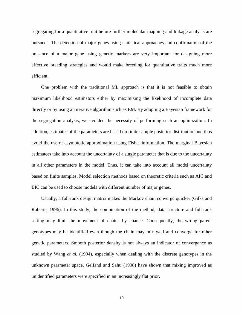
from simulations (Table 3). The Gelman and Rubin plot for a set of initial values (as in N1)

indicated that the burn-in iteration was about 25,000 iterations (see Figure 1). The corrected

scale reduction factors were approximately 1.0, and Raftery dependence factors were found to

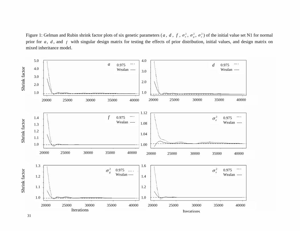
be much less than 5.0. Posterior densities of six genetic parameters, and ,

for a different set of initial values (as in N2) are listed in Figure 2. These numerical

diagnostic summaries (Table 4 and Figure 1) indicated that the chains mix well and there was

2gσ

22 ,,,, gefda σσ 2sσ

15

no severe problem with MCMC convergence. We also found that the prior and initial values

did not have any effects on the Gibbs sampler under the singular design matrix.

When the design matrix was chosen to be of full rank, each individual chain converged

with the Raftery dependence factors less than 5.0. The parameter estimates from the five

different initial value sets N0, N1, N2, N4, and N5 were very good in term of precision. For

the set of initial values N3, however, the estimates of major gene genotype for the 6th parent,

as well as the corresponding genetic parameters, were not correct (see Table 3). As a result,

the 0.975 quantile of corrected scale reduction factors for parameter and were 1.28,

1.29, and 2.87 respectively (see Table 4). This may indicate a possible mixing problem for the

N3 set due to the combination of full-rank design matrix with this data structure. To avoid this

possibility, a normal prior with a singular design matrix was chosen as a model for the further

analysis of our case study.

,, fd 2gσ

5. A case study

The blocking Gibbs sampling method was applied to a progeny data set derived from a 6

parents, half-diallel mating of loblolly pine by the North Carolina State University Tree

Improvement program (Li et al., 1999). Similar to the simulated data, 15 full-sib families

from the diallel mating were planted at 4 different sites with 6 blocks each. Tree heights of

progenies at age 6 were measured as the quantitative trait for this analysis. First, a mixed

linear model was fitted to adjust the site effect t , and block within site effect

. The residuals were used as the phenotypic observation vector . Initial values for GCA,

SCA and variance components were all taken from the estimates from a traditional polygenic

model without the major gene. The prior distribution for

b(t)t +=Y

b(t) Y

a,µ and were normal d ),0(~ 2KN

16

with 4=K . The hyper-parameters for allele frequency were f fα =1 and fβ =1. A singular

design matrix was chosen for the analysis.

The results for two independent chains, with different sets of initial values for

and , were very close to each other using 240,000 iterations (Table 5). The 0.975 quantile

of corrected scale reduction factors for parameters was less than 1.2. The percentage of major

gene effects was estimated as 17% of the total phenotypic variance. The estimated major

genotype of parent 2 was , while that of the others was . The additive effect of the

major gene was 2.3 and the dominance effect was

da,

f

21 AA 22 AA

≈a ≈d -2.3. That is, had 11 AA ≈a 2.3,

had -2.3 and had 21 AA ≈d 22 AA ≈a -2.3. The results indicated that there might be a

detectable recessive major gene controlling the height growth of loblolly pine in this diallel

population, although the effect of the major gene is small compared with the polygenic

effects, which explains about 17% of total phenotypic variance. High estimated GCA values

also indicated that the polygenic component was more important for height growth of loblolly

pine at age 6. Given the limitations of the experimental design and relatively small effect of

the major gene, the major genotypes may not be accurate in this case study. Furthermore, the

validity of the model assumptions and possible interaction of polygenic and major gene

effects may make this genotype interpretation difficult.

6. Discussion

The Bayesian approach with parent-blocking Gibbs sampling has been shown to be effective

in this study for analyzing data from a half-diallel mating design using a mixed inheritance

model. The method can be used successfully to detect major gene segregation, estimate major

17

gene effects and putative genotypes of a major gene for parents and progenies, as well as

polygenic parameters of a quantitative trait. To our knowledge, this is the first statistical

approach that incorporates the polygenic effects of GCA and SCA with a major gene in the

MIM for a diallel mating design. The results from this model have provided a better

understanding of mixed inheritance of quantitative traits in diallel populations, particularly for

tree-breeding.

Although major-gene genotypes detected are putative, based on the statistical

inference, this information of segregation could be valuable for identifying parents with major

genes affecting quantitative traits. The proposed method is based on the existing half-diallel

mating design, and hence it can be used to analyze actual progeny test data for breeding

purposes. By systematically screening progeny test data with this method, putative major

genes, genotypes of parents and progenies, and their probabilities can be estimated. This is in

addition to the polygenic effects of GCA and SCA, and other variance component estimates

from the traditional analysis. The detectable major gene and putative genotypes would be

valuable for selecting materials in an active breeding program. By combining the GCA and

SCA estimates and possible major genotypes, suitable combinations of parents or progenies

can be chosen to provide maximum genetic gains for a breeding program.

The putative genotypes of major genes identified with this method could also be

valuable for molecular mapping experiments by providing a mapping population with a high

probability of segregation for the quantitative traits. This should improve the effectiveness of

searches for QTL in the laboratory and reduce the experimental costs of such a search. Often

no QTLs can be detected due to inadequate segregation in the experimental population. Our

analytical approach can thus be first used to identify parents or families that are most likely

18

segregating for a quantitative trait before further molecular mapping and linkage analysis are

pursued. The detection of major genes using statistical approaches and confirmation of the

presence of a major gene using genetic markers are very important for designing more

effective breeding strategies and would make breeding for quantitative traits much more

efficient.

One problem with the traditional ML approach is that it is not feasible to obtain

maximum likelihood estimators either by maximizing the likelihood of incomplete data

directly or by using an iterative algorithm such as EM. By adopting a Bayesian framework for

the segregation analysis, we avoided the necessity of performing such an optimization. In

addition, estimates of the parameters are based on finite sample posterior distribution and thus

avoid the use of asymptotic approximation using Fisher information. The marginal Bayesian

estimators take into account the uncertainty of a single parameter that is due to the uncertainty

in all other parameters in the model. Thus, it can take into account all model uncertainty

based on finite samples. Model selection methods based on theoretic criteria such as AIC and

BIC can be used to choose models with different number of major genes.

Usually, a full-rank design matrix makes the Markov chain converge quicker (Gilks and

Roberts, 1996). In this study, the combination of the method, data structure and full-rank

setting may limit the movement of chains by chance. Consequently, the wrong parent

genotypes may be identified even though the chain may mix well and converge for other

genetic parameters. Smooth posterior density is not always an indicator of convergence as

studied by Wang et al. (1994), especially when dealing with the discrete genotypes in the

unknown parameter space. Gelfand and Sahu (1998) have shown that mixing improved as

unidentified parameters were specified in an increasingly flat prior.

19

Efficiency of Gibbs sampling depends on the mixing property of the Markov chain,

which in turn is determined by the parameterization used in the model and the sampling

scheme applied. From the consistent results of multiple chains and convergence tests, we

conclude that the chains have mixed well for parent block sampling of genotypes. However, if

the size of progeny population is small and/or the major gene effect is small, mixing may

become a problem even with the parent block sampling. If additional molecular marker

information is included in the model or the overall mean µ in the model is extended to a

vector by including other non-genetic parameters, such as site effects and block within site

effects, the mixing problem may be worse. One possible way to avoid this is to use the hybrid

Markov chain embedding a Hasting or Metropolis updating step in the basic Gibbs sampling

scheme, as used in pedigree analysis (Tierney, 1994). Another way would be to use

Metropolis jumping kernel to make transition between communicating classes (Lin, 1995). A

Bayesian network is also an alternative solution (Lund and Jensen, 1999).

Although only one major gene with two alleles was considered in this study, this

method can be extended to more general situations by considering 2 alleles and/or two or

more major genes. When multiple alleles and genes are involved in the model, many

important issues such as Hardy-Weinberg disequilibrium (among alleles for one gene),

linkage disequilibrium (association among genes), and epistasis (non-allelic interaction)

should be examined. In these cases, model selection can be adopted by means of the Bayes

Factor (Kass and Raftery, 1998), or by means of a predictive loss approach (Gelfand and

Ghosh, 1998).

pn

ACKNOWLEDGEMENTS

20

This research was supported by a grant from the Department of Energy and several industry

members of the North Carolina State University-Industry Cooperative Tree Improvement

Program. The support of the Department of Forestry at the North Carolina State University is

gratefully acknowledged. We thank the North Carolina Supercomputer Center for allowing us

to use its facilities for some computations. We appreciate Drs. Zhao-Bang Zeng, Trudy

Mackay, Rongling Wu, Ben-Hui Liu, and Arthur Johnson for their inputs and helpful

discussions at various stages of this work. We thank the editor and two anonymous reviewers

for their useful comments on this manuscript.

REFERENCES

Brooks, S.P. (1998). Markov chain Monte Carlo method and its application. The Statistician 47, 69-100. Brooks, S.P. and Roberts, G.O. (1998). Convergence assessment techniques for Markov chain

Monte Carlo. Statistics and Computing 8, 319-335. Elston, R.C. and Stewart, J. (1971). A general model for the genetic analysis of pedigree data.

Human Heredity 21,523-542.

Fain, P.R. (1978). Characteristics of simple sib-ship variance tests for the detection of major

loci and application to height, weight and spatial performance. Annuals of Human

Genetics 42,109-120.

Falconer, D.S. and Mackay, T.F.C. (1996). Introduction to Quantitative Genetics. Ed.4, New York: Longman. Gelfand, A.E. and Ghosh, S.K. (1998). Model choice: A minimum posterior predictive loss approach. Biometrika 85(1), 1-11. Gelfand, A.E. and Smith, A.F.M. (1990). Sampling based approaches to calculating marginal densities. Journal of the American Statistical Association 85, 398-409.

21

Gelfand, A.E. and Sahu, S.K. (1998). Identifiability, improper priors and Gibbs sampling for generalized linear models. Journal of the American Statistical Association 94, 247-253. Gelman, A. and Rubin, D.B. (1992). Inference from iterative simulation using multiple sequences. Statistical Science 7, 457-511. Gilks, W.R. and Roberts, G.O. (1996). Strategies for improving MCMC. In Markov Chain

Monte Carlo in Practice (eds. W.R. Gilks, S. Richardson, and D.J. Spiegelhalter), pp. 89-114. London: Chapman & Hall.

Griffing, G. (1956). Concept of general and specific combining ability in relation to diallel

crossing systems. Australian Journal of Biological Science 9, 463-493.

Hallauer, A.R. and Miranda, J.B. (1981). Quantitative genetics in maize breeding. Iowa State Universitypress, Ames, Iowa. P468.

Hoeschele, I. (1988). Genetic evaluation with data presenting evidence of mixed major gene and polygenic inheritance. Theoretical and Applied Genetics 76, 81-92. Huber, D.A., White, T.L. and Hodge, G.R. (1992). The efficiency of half-sib, half-diallel and circular mating designs in the estimation of genetic parameters in forestry: a simulation. Forest Science 38, 757-776. Janss, L.L.G., Van Arendonk, J.A.M. and Brascamp, E.W. (1997). Bayesian statistical

analysis for presence of single gene affecting meat quality traits in a crossed pig population. Genetics 145, 395-408.

Jiang, C.J., Pan, X.B. and Gu, M.H. (1994). The use of mixture models to detect effects of major genes on quantitative characters in a plant breeding experiment. Genetics 136,383- 394. Karlin, S. and Williams, P.T. (1981). Structured exploratory data analysis (SEDA) for determining mode of inheritance of quantitative traits. II. Simulation studies on the effect of ascertaining families through high-valued probands. The American Journal of Human Genetics, 33, 282-292. Kass, R.E., and Raftery, A.E. (1995). Bayes Factors. Journal of the American Statistical Association 90(430), 773-795. Kaya, Z., Sewell, M.M. and Neale, D.B. (1999). Identification of quantitative trait loci influencing annual height- and diameter increment growth in loblolly pine (Pinus taeda L.). Theoretical and Applied Genetics 98,586-592. Kinghorn, B.P., Van Arendonk, J. and Hetzel, J. (1994). Detection and use of major genes in animal breeding. AgBiotech Bews and Information 6(12), 297-302.

22

Knott, S.A., Haley, C.S., and Thompson, R. (1991). Methods of segregation analysis for

animal breeding data: a comparison of power. Heredity 68, 299-311. Le Roy, P., Elsen, J.M. and Knott, S.A. (1989). Comparison of four statistical methods for detection of a major gene in a progeny test design. Genetics, Selection, Evolution 21, 341-357. Li, B. and Wu, R. (1996). Genetic causes of heterosis in juvenile aspen: a quantitative

comparison across intra-and interspecific hybrids. Theoretical and Applied Genetics 93, 380-391

Li, B., McKeand, S.E. and Weir, R.J. (1999). Tree improvement and sustainable forestry – impact of two cycles of loblolly pine breeding in the U.S.A.. Forest Genetics, 6(4), 229- 234. Lin, S., (1995). A scheme for constructing an irreducible Markov Chain for pedigree data. Biometrics 51, 318-322. Liu, J.S., Wong, W.H. and Kong, A. (1994). Covariance structure of the Gibbs sampler with

applications to the comparisons of estimators and augmentation schemes. Biometrika 81 (1), 27-40.

Long, A.D., Mullaney, S.L., Reid, L.A., Fry, J.D., Langley, CH., and Mackay, T.F.C. (1995).

High resolution mapping of genetic factors affecting abdominal bristle number in Drosophilae melanogaster. Genetics 139:1273-1291.

Lund, M.S. and Jensen, C.S. (1999). Blocking Gibbs sampling in the mixed inheritance model

using graph theory. Genetics, Selection, Evolution 31, 3-24. Lynch, M. and Walsh, B. (1998). Genetics and analysis of quantitative traits. Sinauer Association Inc. 321-378. McKeand, S.E., Eriksson, G. and Roberds, J.H. (1997). Genotype by environment interaction

for index traits that combine growth and wood density in Loblolly pine. Theoretical and Applied Genetics 94, 1015-1022.

Mérat, P. (1968). Distributions de fréquences, interprétration du déterminisme génétique

des caracteres quantitatifs et recherche de “géens majeurs.” Biometrics 24, 277-293.

Piper, L.R. and Shrimpton, A.E.. (1989). The quantitative effects of genes which influence metrics traits. in Hill, W.G., Mackay, T.F.C. (eds) Evolution and animal breeding. Reviews on molecular and quantitative approaches in honor of Alan Robertson. Wallingford, CBA Int, 147-151.

23

Remington, D.L. and O’Malley, D.M. (2000) “Evaluation of major genetic loci contributing to inbreeding depression for survival and early growth in a selfed family of Pinus taeda”, Evolution 54,1580-1589

Roberts, G.O., and Sahu, S.K. (1997). Updating schemes, correlation structure, blocking and parameterization for the Gibbs sampler. Journal of Royal Statistical Society Series B 59, 291-317. Smith, B. (2000). Bayesian output analysis program (BOA) Version 0.5.0 Programmer Manual. Tierney, L. (1994). Markov chains for exploring posterior distributions (with discussion). Annual Statistics. 22, 1701-1762. Wang, C.S, Rutledge, J.J., and Gianola, D. (1994). Bayesian analysis of mixed linear models

via Gibbs sampling with an application to litter size in Iberian pigs. Genetics, Selection, Evolution 26, 91-115.

Wang, J., Podlich, D.W., Cooper, M. and Delacy, I.H. (2001). Power of the joint segregation analysis method for testing mixed major-gene and polygene inheritance models of quantitative traits. Theoretical and Applied Genetics 103, 804-816. Wilcox, P.L., Amerson, H.V., Kulman, E.G., Liu, B.H., O’Malley, D.M. and Sederoff, R.R.

(1996). Detection of a major gene for resistance to fusiform rust disease in loblolly pine by genomic mapping. Proceedings of National Academy of Science of the United States of America 93, 3859-3864.

Wu, R. and Li, B. (1999). A multiplicative epistatic model for analyzing interspecific

differences in outcrossing species. Biometrics 55, 355-365. Wu, R. and Li, B. (2000). A quantitative genetic model for analyzing species differences in outcrossing species. Biometrics 56, 1098-1104. Wu, R., Li, B., Wu, S.S. and Casella, G. (2001). A maximum likelihood-based method for mining major genes affecting a quantitative character. Biometrics 57, 764-768. Xiang, B. and B. Li. (2001). A new mixed analytical method for genetic analysis of diallel

data. Canadian Journal of Forest Research 31, 1-8. Zeng, W. (2000). Statistical methods for detecting major genes of quantitative traits using phenotypic data of a diallel mating. Ph.D. dissertation, North Carolina State University, Raleigh, USA. 145p. Zeng, W. and Li, B. (2003). Simple tests for detecting segregation of major genes with

phenotypic data from a diallel mating. Forest Science 49(2), 268-278.

24

Zobel, B.J. and Talbert, J.T. (1984). Applied forest tree improvement. John Wiley and Sons. New York. NY.

25

Table 1: The definitions of the notations used in the mixed inheritance model.

Notation Definition Y a ( x1) vector of progeny observations. n nµ the overall mean, is equal to µ . It can be extended to a ( x1) vector of

fixed non-genetic effects, e.g. site effect and block within site effect. c c

X a ( ) vector with value 1 of overall mean for all progenies. 1nxu a ( x1) vector of random polygenic effects, q q )s,g(u ′′=′ , including

GCAs ( g ) and SCAs ( s ). pn

sng { }pi nig ,...,1, ==′g , GCAs, are assumed to be mutually independent

normal distributions, i.e. .pn

),(~| 22 I0Ng gg σσ 1

2gσ the GCA polygenic variance due to additive polygenic effects.

s { }sj njs ,...,1,' ==s , SCAs, are assumed to be mutually independent

normal distributions, i.e. , sn

),(~| 22 I0Ns ss σσ2sσ the SCA polygenic variance due to dominance polygenic effects.

Z a ( ) incidence matrix of GCA and SCA for all progenies nxqm a (2x1) vector of major gene effects, ),( da=′m . a the additive major genotypic effect.

d the dominance major genotypic effect.

L

⎟⎟⎟

⎠

⎞

⎜⎜⎜

⎝

⎛

−=

0,11,00,1

L , a (3x2) indicator matrix of the major gene effects for major

genotypes. W an unknown ( x3) random incidence matrix of major genotypes at the

single locus for n progenies. n

Tw a (1x3) row vector to form the rows of . =(1,0,0), =(0,1,0), and =(0,0,1),

W 1w 2w

3w T taking values 1, 2, and 3 respectively to represent the major genotype A1A1, A1A2, and A2A2.

e a ( x1) vector of iid errors. e is assumed to be , n ),( 2I0N eσ2eσ the residual variance.

1. N represents the multivariate normal distribution.

26

27

a d

Table 2: The six combinations of initial values (N0-N5) for each of three combinations

of prior and design matrix: Uniform priors for , and µ with singular design matrix,

normal priors for a , , and d µ with singular design matrix, and normal priors for , ,

and

a d

µ with full-rank design matrix to test the effect of prior, initial value, and design

matrix on the mixed inheritance model (MIM) using a blocking Gibbs sampling. In the

MIM model, the polygene background setup was narrow sense heritability of polygenic

inheritance =0.2, the ratio of dominance to additive genetic variance of polygenic

inheritance

2h

r =0.5, and the major gene effect was simulated by 2 , , and .

a d f

Initial value Case \ Parameter a d f N0 (true values) 1.0 0.0 0.2 N1 0.0 0.0 0.1 N2 0.25 0.25 0.2 N3 0.5 0.0 0.3 N4 0.75 0.5 0.4 N5 1.0 0.0 0.5

Parameters a d f 2eσ 2

gσ 2sσ P1 P2 P3 P4 P5 P6

True values 1.0 0.0 0.167 0.595 0.034 0.017 A2A2 A2A2 A2A2 A1A2 A1A2 A2A2

N0 1.03±0.121 -0.07±0.12 0.212±0.102 0.613±0.027 0.017±0.012 0.013±0.008 A2A2 A2A2 A2A2 A1A2 A1A2 A2A2

N1 1.04±0.12 -.008±0.12 0.215±0.103 0.613±0.027 0.017±0.011 0.013±0.007 A2A2 A2A2 A2A2 A1A2 A1A2 A2A2

N2 1.03±0.12 -0.07±0.13 0.215±0.106 0.612±0.028 0.018±0.014 0.013±0.007 A2A2 A2A2 A2A2 A1A2 A1A2 A2A2

N3 1.02±0.13 -0.06±0.13 0.212±0.104 0.614±0.028 0.017±0.010 0.013±0.008 A2A2 A2A2 A2A2 A1A2 A1A2 A2A2

N4 1.03±0.11 -0.07±0.12 0.215±0.107 0.612±0.027 0.016±0.011 0.013±0.008 A2A2 A2A2 A2A2 A1A2 A1A2 A2A2

Uniform prior

N5 1.02±0.12 -0.07±0.12 0.212±0.106 0.614±0.028 0.017±0.011 0.013±0.008 A2A2 A2A2 A2A2 A1A2 A1A2 A2A2

N0 1.04±0.12 -0.08±0.12 0.217±0.108 0.613±0.028 0.017±0.011 0.013±0.007 A2A2 A2A2 A2A2 A1A2 A1A2 A2A2

N1 1.03±0.13 -0.07±0.13 0.215±0.105 0.613±0.028 0.017±0.012 0.013±0.007 A2A2 A2A2 A2A2 A1A2 A1A2 A2A2

N2 1.04±0.12 -0.08±0.13 0.212±0.104 0.612±0.028 0.017±0.010 0.013±0.008 A2A2 A2A2 A2A2 A1A2 A1A2 A2A2

N3 1.01±0.13 -0.05±0.13 0.216±0.107 0.614±0.027 0.017±0.011 0.013±0.007 A2A2 A2A2 A2A2 A1A2 A1A2 A2A2

N4 1.03±0.12 -0.07±0.12 0.215±0.105 0.613±0.026 0.017±0.011 0.013±0.008 A2A2 A2A2 A2A2 A1A2 A1A2 A2A2

Normal prior

N5 1.04±0.11 -0.08±0.11 0.214±0.107 0.611±0.028 0.017±0.028 0.013±0.008 A2A2 A2A2 A2A2 A1A2 A1A2 A2A2

N0 1.02±0.11 -0.07±0.12 0.212±0.106 0.615±0.028 0.015±0.010 0.012±0.006 A2A2 A2A2 A2A2 A1A2 A1A2 A2A2

N1 1.02±0.13 -0.07±0.13 0.215±0.106 0.616±0.027 0.016±0.011 0.012±0.007 A2A2 A2A2 A2A2 A1A2 A1A2 A2A2

N2 1.03±0.11 -0.08±0.12 0.214±0.108 0.614±0.028 0.015±0.010 0.012±0.007 A2A2 A2A2 A2A2 A1A2 A1A2 A2A2

N3 0.95±0.10 -0.20±0.07 0.354±0.123 0.634±0.033 0.100±0.067 0.009±0.006 A2A2 A2A2 A2A2 A1A2 A1A2 A1A1

N4 1.02±0.14 -0.06±0.14 0.216±0.141 0.615±0.105 0.015±0.010 0.012±0.007 A2A2 A2A2 A2A2 A1A2 A1A2 A2A2

Normal prior with full-rank design matrices N5 1.01±0.12 -0.05±0.13 0.216±0.106 0.614±0.106 0.015±0.009 0.012±0.006 A2A2 A2A2 A2A2 A1A2 A1A2 A2A2

MC error 2 0.006 0.006 0.002 0.0006 0.0003 0.0002

Table 3: Estimated means, and standard deviations of posterior densities for six genetic parameters (a, d, f, , , ), and genotype

estimates of six parents (P

2eσ 2

gσ 2sσ

1-P6) for testing the effects of prior distribution, initial value, and design matrix on the mixed inheritance

model. In the MIM model, the polygene background setup was =0.2, 2h r =0.5, and the major gene effect was simulated by 2 =2.0,

=0.0 and =0.2 (actual value is 0.167). There were six runs, N0 to N5, for each of three cases.

a

d f

1: mean ± standard deviation of the parameter estimate from the Gibbs sample with lag=5; 2: There is one MC error for each Chain. Because the values for each parameter are so close, only an average value is listed here.

28

29

2eσ 2

gσ 2sσ

2

Table 4: Convergence diagnostics of the six parameters, a, d, f, , , , for testing

the effects of prior distribution, initial value, and design matrix on the mixed inheritance

model. In the MIM model, the polygene background setup was h =0.2, r =0.5, and the

major gene effect was simulated by 2 =2.0, =0.0 and =0.2 (actual value is 0.167).

There were six runs, N0 to N5, for each of three cases.

a d f

2eσ 2

gσ 2sσParameters a d f

Est 1.00 1.00 1.00 1.00 1.00 1.00 CS Reduction

Factor1 .975 1.01 1.01 1.00 1.00 1.00 1.00 N0 12.2(1.7)3 3.0(1.5) 1.0 1.1 1.1 1.0 N1 9.8(2.0) 5.4(1.7) 1.0 1.3 1.1 1.1 N2 10.4(1.7) 4.9(1.3) 1.0 1.3 1.0 1.2 N3 5.0(1.7) 5.5(1.5) 1.0 1.2 1.0 1.0 N4 8.2(3.3) 6.3(2.6) 1.0 1.2 1.2 1.0

Uniform prior

Raftery Dependent Factor2

N5 6.2(1.5) 5.8(1.1) 1.0 1.2 1.0 1.2 Est 1.00 1.00 1.00 1.00 1.00 1.00 CS Reduction

Factor .975 1.01 1.01 1.00 1.00 1.00 1.00 N0 13.0(3.1) 8.7(2.0) 1.1 1.3 1.0 1.2 N1 13.6(2.2) 7.6(1.5) 1.1 1.3 1.1 1.2 N2 19.9(4.3) 7.1(1.5) 1.0 1.0 1.2 1.0 N3 4.4(1.3) 4.6(1.5) 1.2 1.2 1.0 1.1 N4 4.9(1.2) 8.2(1.8) 1.1 1.1 1.1 1.2

Normal prior

Raftery Dependent Factor

N5 5.4(1.3) 4.6(1.5) 1.0 1.3 1.3 1.1 Est 1.04 1.11 1.12 1.04 1.98 1.03 CS Reduction

Factor .975 1.09 1.28 1.29 1.11 2.87 1.08 N0 5.2(1.5) 5.7(1.3) 1.0 1.1 1.0 1.0 N1 6.4(1.7) 4.9(1.3) 1.0 2.0 1.2 1.2 N2 5.9(1.5) 4.7(1.3) 1.1 1.2 1.2 1.2 N3 9.1(2.2) 3.2(1.3) 1.0 1.3 2.6 1.0 N4 31.1(5.9) 6.2(1.3) 1.0 1.3 1.2 1.1

Normal prior with full-rank design matrices

Raftery Dependent Factor

N5 8.0(1.7) 7.4(3.3) 1.1 1.2 1.2 1.2

lag=5 in the regular base because of strong autocorrelation;

and Probability = 0.9.

3: The dependent factor in the parenthesis was calculated by using lag=30, instead of

2: Raftery Dependent Factor is calculated under Quantile = 0.025, Accuracy = ± 0.05,

1: CS Reduction Factor: corrected score reduction factor;

Table 5: Estimated means and standard deviations of posterior densities for seven genetic parameters ( , , , , , , ), and

general combining ability (GCA) (

a d f 2eσ 2

gσ 2sσ 2

mσ

61 gg − ) and major gene genotypes of six parents ( 61 PP − ) for the diallel from Bayesian based

segregation analysis. There were two independent runs, chain 1 and chain 2.

Genotype P1 P2 P3 P4 P5 P6

Chain 1 22 AA (.95)1

21AA (.90) 22 AA (.86) 22 AA (.84) 22 AA (.97) 22 AA (.91)

Chain 2 22 AA (.97) 21AA (.86) 22 AA (.82) 22 AA (.80) 22 AA (1.0) 22 AA (.93)

GCA g1 g2 g3 g4 g5 g6

Chain 1 1.30±0.812 -0.88±0.64 0.03±0.69 -0.45±0.67 0.66±0.67 -0.27±0.75

Chain 2 1.53±0.92 -0.91±0.62 -0.05±0.71 -0.48±0.68 0.84±0.76 -0.26±0.76

Parameter a d f 2eσ 2

gσ 2sσ 2

mσ 2pσ

22 / pm σσ

Chain 1 2.29±0.65 -2.31±1.05 0.33±0.16 6.96±0.25 0.96±0.92 1.41±0.90 2.18±1.50 12.47 0.175

Chain 2 2.17±0.65 -2.25±0.78 0.37±0.17 6.91±0.27 1.12±1.09 1.29±092 2.16±1.41 12.60 0.171

1: Probability of this genotype

2: the estimated mean ± standard deviation from the Gibbs samples with lag=5

30

31

Shrin

k fa

ctor

Shrin

k fa

ctor

Figure 1: Gelman and Rubin shrink factor plots of six genetic parameters a d f 2e

2g

2s ) of the initial value set N1 for norma

prior for a d , and f with singular design matrix for testing the effects of prior distribution, initial values, and design matrix onmixed inheritance model.

( , , , , , l ,

σ σ σ

Iterations

20000 25000 30000 35000 40000

20000 25000 30000 35000 40000 20000 25000 30000 35000 40000

1.3

2

1. 1.1 1.0

1.4

1.3

1.2

1.1

1.0

f 0.975 … .

Wealan ---- 2eσ 0.975 … .

Wealan ----

1.12 1.08 1.04 1.00

20000 25000 30000 35000 40000 20000 25000 30000 35000 40000

2sσ 0.975 … .

Wealan ---- 2gσ 0.975 … .

Wealan ----

1.6 1.4 1.2 1.0

Iterations

20000 25000 30000 35000 40000

a 0.975 … .

Wealan ---- 0.975 … .

Wealan ---- d

Shrin

k fa

ctor

4.0 3.0 2.0 1.0

5.0 4.0 3.0 2.0 1.0

Figure 1: Gelman and Rubin shrink factor plots of six genetic parameters ( , , , , , ) of the initial value set N1 for normal prior for , , and with singular design matrix for testing the effects of prior distribution, initial values, and design matrix on mixed inheritance model.

a da d f

2eσ 2

gσ 2sσf

32

f

Figure 2: Posterior densities of six genetic parameters ( , , , , , ) of the initial value set N1 for normal prior for ,

, and

a d f 2eσ 2

gσ 2sσ a

d µ with singular design matrix were used for the mixed inheritance model. The horizontal dots are the Gibbs sample

values for the parameter.

3 2 1 0

0.4 0.6 0.8 1.0 1.2 1.4 - 0.6 - 0.4 -0.2 0.0 0.2 0.4 0.6

0.0 0.2 0.4 0.6

Parameter value

0.00 0.05 0.10 0.15 0.20

Parameter value0.00 0.02 0.04 0.06 0.08 0.10 0.12 0.14

3 2 1 0

60 40 20 0

12 8 4 0

f

0.50 0.55 0.60 0.65 0.70 0.75

2gσ 2

sσ

a d

2eσ

Den

sity

4 3 2 1 0

Dty

ensi

50

30

10 0

De

tyns

i