A BIOLOGICAL NEEDS ASSESSMENT FOR

ANADROMOUS FISH IN THE SHASTA RIVER

SISKIYOU COUNTY, CALIFORNIA

Prepared by the

California Department of Fish and GameNorthern California-North Coast Region (Region 1)

Northern Management Area (Area 2)601 Locust Street

Redding,, California 96001

July 1997

Table of Contents

I.

II.

III

IV.

V.

BACKGROUND . . . . . . . . . . . . . . . . . . . . . . .Physical Setting ....................Water Development ...................

SALMON AND STEELHEAD IN THE SHASTA RIVER ........Chinook Salmon .Coho and Steelhead : : : : : : : : : : : : : : : : : : :Life History. ......... 1 ...........

Fall Chinook ...................Coho Salmon ....................Steelhead .....................

. HABITAT NEEDS .....................Habitat Criteria ....................

Water velocity ..................Depth . . . . . . . . . . . . . . . . . . . . . . .Substrate .....................Temperature ....................

CURRENT HABITAT DEFICIENCIES AND THREATS ........Flows . . . . . . . . . . . . . . . . . . . . . . . . .Water Temperature ...................Dissolved Oxygen ....................Dam and diversion structures ..............Grazing . . . . . . . . . . . . . . . . . . . . . . . .Wells . . . . . . . . . . . . . . . . . . . . . . . . .Harvest ........................

RECOMMENDATIONS .....................Research Needs .....................Habitat Improvement ..................

VI. LITERATURE CITATIONS . . . . . . . . . . . . . . . . . . . .

. 1

. 1

. 1

. 3

. 44

'10101212

131414141515

1515191920212223

252526

27

I. BACKGROUND

Physical SettingThe Shasta River originates within the higher elevations of theEddy Mountains lying southwest of

California.the town of Weed in Siskiyou

County, It flows for approximately 50 miles in anortherly direction, passing through the Shasta Valley. Afterleaving the valley, i t enters a steep-sided canyon where it flowsfor a distance of 7 rive r miles before emptying into the KlamathRiver 176.6(Figure 1).

river miles (RM) upstream from the Pacific Ocean

Numerous springs and a number of small tributary streams enter theShasta River as it passes through the Shasta Valley. Majortributaries include Parks Creek, Big Springs Creek, Little ShastaRiver, and Yreka Creek. Water diversions for agricultural andstock water needs exist on these and several other smallertributary streams, reducing or eliminating their flow contributionto the Shasta River, particularly during the main irrigation seasonwhich runs April 1 to October 1. The Shasta River was dammed at RM37 to form Dwinnell Reservoir (Lake Shastina) in 1928.

The Shasta River subbasin consists of approximately 507,000 acres.About 28 percent of this acreage (141,000 acres) is irrigable andexists primarily below Dwinnell Dam (DWR, 1964). The climate ofthe Shasta Valley is characterized by warm, dry summers and coolwet winters. Precipitation averages 12 to 18 inches annually with75 to 80 percent of it occurring between October and March. Thelength of the average growing season is about 180 days (DWR, 1964).

Water DevelopmentWater development within the Shasta subbasin began in earnest withthe arrival of the gold miners in the late 1800s. After the goldrush, agricultural development resulted in additional and moreextensive use of water from the Shasta River. Dwinnell Dam wasconstructed in 1928 to capture winter and early spring run-off.Originally, the dam measured 1,265 feet in length, was 98 feet highand had an effective storage capacity of approximately 34,000 acrefeet. In 1955, the height of the dam was raised which increasedthe total storage capacity to 50,000 acre-feet. When full, thereservoir has an average depth of 22 feet with a-maximum depth of65 feet and a surface area of 1,824 acres (2.85 mi2). Wales (1951)estimated that construction of Dwinnell dam eliminated access toabout 22 percent of the total spawning habitat formerly availableto salmon and steelhead and approximately 17 percent of thedrainage area.

Seven major diversion dams and several smaller dams or weirs existon the Shasta River below Dwinnell Dam. Numerous diversions and‘associated dams exist on other major tributaries as well, including

AA R.5W. R.4W. 1

Location Map

T.45N

Diversion Dams

T.44N

T.431

T.42N

~xilometers0 .5 1 2

Figure 1 . Shasta Valley showing location of major water diversion structures and the ShastaRiver Fish Counting Facility.

2

Big Springs Creek, Little Shasta River and Parks Creek (Figure 1).When all diversions are operating,and in the case of

flows are substantially reducedthe Little Shasta River, stream flows cease

entirely in the lower several miles of stream during the summer andfall period.

Prior to the construction of Dwinnell Dam, four water serviceagencies had been formed in the Shasta Valley. The Shasta RiverWater Association (SRWA) was formed in 1912 and obtained a 1932water appropriation notice that same year for 42 cubic feet persecond (cfs) for the period April 1 through October 1 each year.The SRWA serves the west side of the Shasta Valley near the town ofMontague. The Grenada Irrigation District (GID) (formerly known asthe Lucerne Water District) was formed in 1921 and has a right to40 cfs for the period April 1 through October 1. Prior downstreamwater rights have limited the ability of GID to take its fullentitlement in some years. The GID serves about 1,800 acreslocated west of the town of Grenada.District (BSID), formed in 1927,

The Big Springs Irrigationhas a 30 cfs right for water from

Big Springs lake and serves about 3,600 acres north of the lake.Since the late 1980s, BSID has used ground water in lieu of waterdiverted from Big Springs Lake.

The Montague Water Conservation District (MWCD), also known as theMontague Irrigation District, was formed in 1925. As a result ofa 1932 adjudication, MWCD obtained appropriative rights for winterstorage of the Shasta River and Parks Creek in Lake Shastina tomeet irrigation needs in the Little Shasta Valley and the northeastportion of the Shasta Valley during the April 1 through October 1irrigation season. Except during above normal water years, whenLake Shastina is full, the only flow release made to the ShastaRiver below the dam are those intended to satisfy the needs ofseveral small users immediately downstream of the dam.

Since 1934, available water resources in the Shasta River have beenapportioned by the California Department of Water Resources (DWR)Watermaster Service in accordance to a 1932 statutory adjudication(Decree No. 7035). However, riparian water users along the ShastaRiver below Dwinnell Dam were not included in this adjudication andare not regulated by the watermaster.

II. SALMON AND STEELHEAD IN THE SHASTA RIVER

The Klamath River system ranks first in California in the number ofcoho salmon (Oncorhynchus kisutch) and steelhead (0. mykiss)produced and second after the Sacramento River system in the numberof chinook salmon (0. tschawytscha) produced annually (Leidy &Leidjj, 1984). Historically, spring-run chinook salmon comprised the major portion of the chinook salmon run entering the Klamathuntil habitat destruction led to near extirpation of that raceduring the early part of this century (Snyder 1931). Fall chinook

3

salmon have since predominated in the Klamath River basin and isthe only chinook race believed to currently exist in the ShastaRiver basin. Coho salmon and fall and winter-run steelhead stilloccur in the Shasta River although little is known regarding theirpresent abundance.

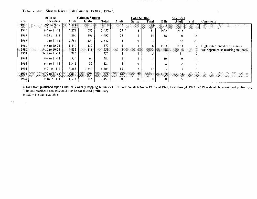
Chinook SalmonThe California Department of Fish and Game (DFG) has monitored theShasta River fall chinook salmon runs since 1930. The Shasta RiverFish Counting Facility (SRFCF) was originallyoperated near the mouth at approximately 0.5 RM).

installed and

and 1957,Between 1938

the SRFCF was moved 6.5 miles upstream from the KlamathRiver to an existing steelhead egg taking station. Sinceconsiderable Salmonid spawning is known to occur in the lower 6.5river miles, actual spawner escapement was probably higher duringthis period than reported. Starting in 1958, the weir was movedback to its original, and current location.

Chinook salmon counts have ranged from nearly 82,000 fish in 1931to just 533 (415 adults) in 1990 (Table 1). Between 1960 and 1992,the overall decline in returns of chinook to the Shasta Rivercontinued (Figure 3). However, during the years 1993 and 1995, thereturns of fall chinook salmon increased coincident with thecessation of drought conditions and a total ban on ocean commercialharvest within the Klamath Management Zone. Ocean and in-riversport harvest as well as tribal net harvest allocations were alsoseverely restricted between 1990 and 1995.

In 1995, over 13,500 fall chinook salmon returned to the ShastaRiver. Of this number, an estimated 5.8 percent (791 salmon) wereIron Gate Hatchery (IGH) strays (based on coded-wire tag expansionsand observed hatchery marks). Although the 1995 run wasconsiderably larger than the runs observed during the early 1990'sand was 1.5 times larger than the previous 35-year average, it wasonly about a third of 1963 and 1964 run totals (Figure 3). Thepreliminary fall chinook salmon run size estimate for the 1996season is 1,450; less than 11 percent of the previous years run.

Coho and SteelheadInformation for coho salmon and steelhead observed at the SRFCF hasbeen reported since 1932. In all but a few cases, the numbersreported do not represent the entire run since field activitieswere normally terminated before complete counts could be made.Available information for coho salmon and steelhead as well as thelength of the trapping season is presented in Table 1. Coho salmonand steelhead observed at SRFCF since 1957 are shown in Figures 4and 5.

Spawning LocationsChinook salmon spawning takes place in the Shasta River between theKlamath River confluence and Yreka-Ager Road (RM 10.5). Spawningalso occurs in a reach extending from about one miie below the Big

7

1961

i I I

1971

/ /1976 1981 1986 1991 nrg

Figure 2. Shasta River fall chinook salmon escapement, 196 1 - 1995. Second column from far right column is the35-year average. Far right cohmm is preliminary 1996 run size.

rI !

0 No. of grilse

No. of adults

I

i /

1958 1963 1968 1973 1978 1983 1988 1993

Figure 3. Number of coho salmon observed at the Shasta River Fish Counting Facility, 1957 to 1996. Years 1978through 1982 were years of extended weir operations.

8

2000

1500 t

500

0

1958 1963 1968 1973 1978 1983 1988 1993

-

-

-

-

Figure 4. Number of steelhead observed at the Shasta River Fish Counting Facility, 1957 to 1996. Years 1978through 1982 were years of extended weir operations_

Springs confluence (RM 30) to Louie Road (RM 31.3) and in the lowermile of Big Springs Creek. Very little spawning occurs in theShasta Valley due to the paucity of gravel (DWR 1981, DFG files).During years of adequate streamflow, salmon are able to spawn inthe Shasta River above Louie Road in the vicinity of Parks Creekand in Parks Creek (DWR, 1981, DFG files).

In 1937, the DFG fish counting station was moved from the mouth toapproximately RM 6.5. Between 1937 and 1957, the DFG estimatedthat approximately one third of the chinook salmon spawning runoccurred below the relocated counting station and two-thirdsspawned above. In 1981, the DFG (DWR, 1981) estimated that two-thirds of the spawning now occurs in the lower 8 river miles. In1995, chinook salmon were observed in Little Shasta creek andspawning in Yreka Creek.

Very little information is available regarding the spawningdistribution of coho salmon and steelhead in the Shasta subbasin.Skinner (1959) reporrted that adult steelhead spawn in the lowerseven miles of the Shasta River, in Big Springs Creek, in the mainShasta River above Big Springs Creek and in Parks Creek when flows-were adequate. Steelhead are also known to spawn in the lowerthree miles of Yreka Creek. Skinner suggested that since coho

9

salmon have similar spawning requirements as do steelhead, cohosalmon probably spawn in the same areas. Additional andcomprehensive monitoring of the timing and distribution of spawningis needed to understand spawning patterns in the Shasta subbasin.

Fall ChinookLife History

Adult fall chinook salmon begin entering the Klamath River in lateJuly, ascending the Klamath River and its tributaries betweenAugust and December, depending on the tributary and its location inthe drainage. Chinook salmon begin entering the Shasta River inSeptember with adult immigration continuing into November (Figure5) . The majority of spawning occurs during October and November.The period of egg incubation begins as soon as spawning occurs andis usually completed before March (Leidy & Leidy, 1984).Emergence, the period in which developing fish swim up through thegravel and enter the stream, takes place late January throughMarch.

Three chinook salmon early life history phases involving riveroutmigration have been identified within the Klamath River basin(KRBFTF, 1991). The three phases or life history "types" areoutlined below.

Type I Outmigration occurs in spring within several months offry emergence.

Type I I Juveniles spend their first spring and summer in streamand outmigrate in the fall.

Type III Juveniles spend an entire year in the stream and out-migrate in the spring of the following year.

Juvenile salmon ready to descend their natal streams and enter theestuary and ocean are called "smolts". Smoltification is a processinvolving chemical/hormonal changes in the body that prepare thefish for a saltwater environment. Young-of-the-year (YOY) smoltsfrom the Shasta River system generally outmigrate between Februaryand mid-June (Type 1 life history phase) (Leidy and Leidy, 1984).Through the use of fyke traps, Jong, (1994) found YOY chinookleaving the Shasta River as early as January through and as late aslate-June.

In recent years -we have observed juvenile chinook residing in theShasta River beyond June. This indicates that not all juvenilechinook are following the "Type I" outmigration pattern. Arelatively smaller outmigration of juvenile chinook salmon smoltshas been noted in the fall. It is unclear whether this means that"Type II" or "Type III" outmigration tendencies exist among ShastaRiver chinook or if environmental conditions and irrigationdiversion structures cause fish to remain in the upper

10

-Figure 5-

Spawning, egg incubation, and migration periods of anadromous fish for the Shasta River.

UPSTREAM MIGRATION ADULTS

SPAWNING PERIOD

EGG INCUBATION PERIOD

DOWNSTREAM MIGRATION JUVENILES

UPSTREAM MIGRATION ADULTS

SPAWNING PERIOD

EGG INCUBATION PERIOD

DOWNSTREAM MIGRATION JUVENILES

UPSTREAM MIGRATION ADULTS

SPAWNING PERIOD

EGG INCUBATION PERIOD

1 I

1 I I

1 I1

I I(Fall) CHINOOK SALMON

COHO SALMON

DOWNSTREAM MIGRATION JUVENILES I I I I

am.1 Feb IMar.IApr.[ May IJunelJulyl Aug.1 Sep.lOct.lNov.[ Dec.

STEELHEAD

portion of the river beyond their normal tendency to do so.Additional studies are needed to evaluate Shasta River chinooksalmon rearing and outmigration patterns.

After descending the Shasta River, fall chinook salmon enter theKlamath River en route to the estuary and ultimately the PacificOcean. In the ocean, chinook salmon normally mature at three tofive years of age, although a small portion of each year's broodreturn are sexually mature two-year old males known as “jack“ or"grilse" salmon.

Coho SalmonLittle is known regarding the number of spawners, migrationpatterns and behavior of coho salmon produced in the Shasta River.We believe, however, these fish follow the migration patterns andemulate the behavior of coho salmon studied in other areas of theKlamath River basin and elsewhere.

Nearly all adult coho enter the Klamath River from mid-Septemberthrough January as three-year old fish (USFS, 1972). A very smallnumber of coho return to spawn at age four. Coho residing in theocean for less than one year before returning to the Klamath Riverbasin come back at age two as grilse. Coho generally selectsmaller tributaries for spawning with spawning occurring fromNovember through January. Egg incubation begins in November withthe initiation of spawning activity and continues through March.Hatching occurs in one to three months, depending on watertemperature, with fry emergence occurring from February throughmid-May (Figure 5).

Juvenile coho salmon remain in freshwater for approximately oneyear prior to outmigrating as yearling smolts between February andmid-June. Within the Klamath River basin, peak outmigrationactivity occurs during April and May (Leidy & Leidy, 1984).

SteelheadRuns of steelhead identified in the Klamath River basin are spring-run (better known as summer steelhead), fall-run and winter-run.The runs are classified based on the season of the year they enterthe Klamath River as adults. Spring-run, or summer steelhead, donot presently occur in the Shasta River.similar lif

Because of their verye histories both fall- and winter-run steelhead will be

discussed together.

The initial stages of the fall-run begin with the movement of smallmigrants called "half-pounders" during the months of August throughOctober. Half-pounders spend one to three years in a freshwaterenvironment and less than a year in the ocean. These small,immature fish spend several months in the Klamath River and its major tributaries tending to remain primarily in the lower portionof the Klamath River basin below the confluence of the Scott River.

12

The half-pounder run is unique in that it occurs in large numbersin only two river systemss in California (Klamath and Eel rivers)and in Oregon's Rogue River (Rankel, 1978).

The arrival of greater numbers of larger, sexually mature steelheadin October and November marks the start of the fall-run. Thewinter-run steelhead migration overlaps the fall-run, with winter-run fish beginning to enter the Klamath River in December. Themajority of the winter-run steelhead enter their natal streams tospawn from December through April. Steelhead spawning takes placein the Shasta River basin beginning around mid-December andcontinues through April (Leidy and Leidy, 1984) (Figure 5). It isuncertain whether fall-run and winter-run steelhead spawn atdifferent times or select different locations for spawning withinthe Shasta subbasin. Steelhead may spawn more than once duringtheir life, generally returning to t h e ocean after spawning.

Steelhead egg incubation occurs in the Shasta River from mid-December through mid-June (Leidy and Leidy, 1984). The actualincubation period is dependent on water temperature. Coldwatertemperatures impede egg development and delay hatching. Emergenceof Shasta River steelhead alevins generally occurs between Marchand June (Leidy and Leidy, 1984) . Based on DFG trapping results inthe Shasta River during the winter and springs of 1986-1989 and1992 (Jong, 1994 and DFG files, Yreka), steelhead emergence canoccur as early as the first week of February.

Juvenile steelhead usually spend one to three years (most twoyears) in their nursery stream environment before outmigrating tothe ocean. Size appears to be a determining factor forsmoltification and outmigration. Smoltification generally occurswhen fish reach approximately six inches in length (USFS 1972 asreported in Leidy and Leidy). Outmigration of steelhead smolts isknown to occur between February and June. After one to four yearsin the ocean, steelhead will enter the Klamath River system fortheir first spawning with the possibility of additional runs insubsequent years (Leiciy and Leidy, 1984).

III. HABITAT NEEDS (Physical/Biological)

Anadromous salmonids change their habitat requirements during theirresidency within the Shasta River subbasin. Anadromous fish needholding, spawning, incubation and juvenile rearing habitat. Theterm habitat refers to the physical attributes of the stream (i.e.,pools, runs, riffles, instream structures, etc.) and streambed type(i.e., sand, gravel, cobble, rubble and boulder dominated).Habitat also refers to food availability, water quality (i.e.,temperature, dissolved oxygen, macronutrients, etc.) and quantity(i.e., habitat space availability).

13

Habitat variables are generally discussed separately in terms oftheir impacts on fish. In reality, fish respond to the combinedeffects of physical, chemical, and biological variables in theirsurroundings. It is a mix of these environmental factors whichsets the carrying capacity of a particular stream. As one or moreof these habitat variables are altered, the carrying capacity ofthe stream is changed. A single sublethal environmental conditionmay illicit only a minor stress response, however, when combinedwith other sublethal conditions may lead to more serious problemsor even death. This synergistic effect may be far more damagingthan the effects of each sublethal factor acting separately.

Habitat CriteriaGenerally, salmon and steelhead require stream habitats that meeta narrow range of water velocity, depth, temperature and substratecriteria.

Water velocitySuitable water velocity is important for migration, spawning,incubation, and rearing of salmonids. It is usually considered amore important parameter than depth for determining the hydraulicsuitability of a spawning area. Velocity also helps determine theamount of water which will pass over incubating eggs. Optimalspawning velocity for chinook salmon in the Central Valley streamsof California is 1.5 feet per second (fps) with a range of 1.0 fpsto 3.5 fps (Reynolds et al., 1990). Steelhead prefer slightlyfaster water (2.0 fps, range 1.0 to 3.6 fps) (Bovee, 1978 asreported in McEwan and Jackson, 1996).

Velocity is also an important factor in determining where youngsalmonids rear. The ability of fish to maintain position in thecurrent is related to their size and swimming ability. Largerjuveniles are more capable of maintaining their position in fasterwater than newly emergedrelatively slower waterUSFWS, 1983).

fry which tend to stay-near the shore inChapman and Bjornn, 1968 as reported in

Salmon usually spawn at a depth ranging from 0.5 to 3 .O feet(Reynolds et al., 1990), although they can spawn at much greaterdepths. Steelhead prefer depths ranging from 0.5 to 2.0 feet forspawning (Bovee, 1978 as reported in McEwan and Jackson, 1996).Chinook salmon juveniles generally prefer deeper water thansteelhead in the same stream (Chapman and Bjornn, 1968 as reportedin USFWS, 1983).

Depth directly affects the amount of rearing space available. Inshallow streams, space may limit rearing capacity causing fish toredistribute downstream or outmigrate before they are ready..Literature reviewed by Pauley et al. (1986) indicates water depthrequired by rearing salmonids may be closely tied to aquatic insect

14

(food) production. In stream environments, areas of highestinvertebrate production are those associated with riffles whenflows and substrate are adequate.

Adult upstream migration is triggered by increases in river levelsand changes in water temperature (USFWS, 1983) and insufficientwater depth can become a barrier to that migration. Deep pools arerequired by returning spawners for holding and resting.

SubstrateTo allow excavation of the redd (area of gravel in which the femalesalmon or steelhead lays her eggs) and to permit water and itsdissolved oxygen to percolate through to incubating eggs, substratecomposition must be low in fines and sand. Generally, 85 percentof incubating Salmonid eggs will suffer mortality when 15 to 20percent of the voids (interstitial gravel spaces) become filledwith sediment (Bell 1990). Chinook salmon prefer substrate whichconsists mostly of gravel from 0.75 to 4.0 inches in diameter withless than 20 percent fines (by volume) (Reynolds et al., 1990).Steelhead prefer a similar sized substrate with less than 5 percentfines (McEwan and Jackson, 1996).

Water temperature influences the development and survival ofsalmonids by affecting different physiological processes such asgrowth and smoltification. Water temperature also affects thefishes' migration timing, ability to cope with predation, diseaseand exposure to contaminants. The preferred spawning temperaturefor chinook salmon is 52°F with acceptable upstream migrationtemperatures ranging between 57o and 67°F (Reynolds et al., 1990).Water temperatures above 70°F can delay adult migration (Bell1990). Temperatures at which 100 percent mortality of Shasta RiverSalmonid stocks occurs have not been determined although Reisnerand Bjomn (1979) report upper and lower lethal temperature levelsfor chinook aretemperatures forand lower lethal(Bell, 1990).

Preferred water temperatures for steelhead vary depending on lifestage and stock characteristics. Generally, for adult migration,egg incubation and juvenile rearing, temperatures between 45o and52oF are desired. Optimal temperatures for spawning range between39o and 52°F (McEwan and Jackson, 1996).upper lethal limit is 75°F.

Bell (1990) reports the

79.6oF and 33.5oF, respectively. Preferred watercoho salmon range between 38°F and 69°F while uppertemperature levels are 78oF and 32oF, respectively

15

IV. CURRENT HABITAT DEFICIENCIES AND THREATS

FlowsStreamflow, a function of water velocity and depth, is an importantconsideration when dealing with anadromous fish. The United StatesGeological Survey (USGS) has collected streamflow records for theShasta River since 1912. Initially, the stream gauge was locatednear the town of Montague and flow information was collected foryears 1912-1913, 1917-1921 and 1924-1933. Since 1933 theCalifornia Department of Water Resources (DWR) water-masteroperates this gauge only during the irrigation season. In October1933, the USGS began operating a new gauge located near the town ofYreka approximately 0.5 miles above the Klamath River confluence.The USGS located this new gauge approximately 14.5 miles downstreamof the old gauge. With the exception of the period December 1941through December 1944, this new gauge has been in continuousoperation.

Construction of Dwinnell Dam and increased water diversions foragricultural, stockwater, recreational and domestic uses haveresulted in changes to the annual flow regime of the Shasta River.In general, higher base flows existed in the river prior to theconstruction of Dwinnell Dam than exist currently for the spring,summer and early fall periods. Prior to Dwinnell Dam, mean dailyflows in the Shasta during the spring (April through June) averaged132 cfs. During the years 1985 through 1994, April through Juneflows averaged 87 cfs; a 34 percent reduction during the smoltsalmon outmigration period. Average summer flows (July and August)for predam years is 42 cfs while during recent years it hasaveraged 28 cfs. Mean daily flows for the month of September forpre and postdam conditions are 79 and 61 cfs, respectively (Figure6).

Under current conditions, flow reductions caused by the start ofthe irrigation season are more dramatic than the gradual flowdeclines observed for predam years. During the drought year of1992, flows dropped from 105 cfs on March 31 to 21 cfs on April 5due to the start of the irrigation season. Documented fish killsresulted.

It is likely that greater flow differences exist than thosedescribed above because of the location of the two gauges used forthis comparison. Flows measured near the mouth account for nearlyall of the accretions to the river while those measured 14.5 milesupstream at the old site would not. The reader is also remindedthat considerable water development had already occurred in theShasta Valley prior to the initiation of flow measurements by theUSGS and the construction of Dwinnell Dam.

In dammed and diverted streams like the Shasta River, flows andresultant water velocity changes may be important factors affectingjuvenile salmon outmigration and survival. Studies in the SanJoaquin system of California have shown that survival of chinooksalmon smolts is positively correlated with increases in flow

16

450

400

350

300

Pre Dwinnell- - - Post Dwinnell

I

.

Figure 6. Mean daily flows for the Shasta River averaged for a ten year period pre and post Dwinneil Dam construction (smoothed by a runningaverageof 3). Years used for pre Dam average: 1912-1 3, 19 17-2 1 1924-26. Post dam construction years used were 1985 through 1 994

inclus i ve.

(Kjelson and Brandes, 1989). DFG studies showed decreaseddensities of rearing salmon in the Stanislaus and Tuolumne riversand increases in their catch in the Sacramento/San Joaquin Deltanear Mossdale following increased releases from Goodwin and DonPedro dams (Pisano et al., 1992). Monitoring juvenile salmonmovement in the lower Shasta River during the spring of 1993 showedincreases in their catch coincident with increased flow (andvelocity) resulting from a planned and organized cessation of waterdiversions by local irrigators.

In some years, the onset of the chinook salmon run into the ShastaRiver appears to be tied closely to the end of the main irrigationseason (October 1) and resultant increases in flow (Figure 7).coots (1957, 1958) observed a similar relationship between flowchanges in the Shasta River and adult fall chinook salmon runtiming in the late 1950's. Between i933 and 1934, Brown (1938)reported that chinook salmon began their migrationRiver during the first two weeks of September.conditions, the start of the run has shifted to(Figure 7).

into the ShastaUnder presentlate September

Flows can affect the distribution of spawning in the Shastasubbasin. Low flow conditions limit the ability of fish to accessand utilize the Shasta River above Louie Road. Skinner (1959)noted that, with few exceptions, flows between Dwinnell Dam andLouie Road (Big Springs) have been inadequate in providing suitable

O 140 iII

1t 120 ,

,- 100 z

c

!80 ;

I 2,60 IL

Figure 7. Number of chinook salmon counted by day and mean daily flows for the Shasta River averaged for theyears 1992 through 1994.

18

spawning habitat. Salmon carcass surveys conducted by the DFG in1980, 1993 and 1994 did not include the Shasta River above theLouie Road because of low flows. A check of the Shasta Riverbetween Parks Creek (RM 32) and the Hole in the Ground Ranch (RM34) in 1994 revealed that no salmon utilized this area despite anapparent abundance of gravel. During the 1995 and 1996 seasons,years in which observed flows were higher than the previous fewyears, numerous redds were counted in this same area and in thelower half-mile of Parks Creek. In 1995 and 1996, the DFG alsoobserved salmon spawning in Yreka Creek, near the town of Yreka.

Salmon and steelhead produced in the Big Springs area (RM 30) andabove have much greater rearing opportunity (ie, >20 river miles)than fish produced in the lower section. Because of this, chinookand, particularly coho and steelhead originating from the BigSprings area, would likely be larger at outmigration than salmonidsoriginating from the canyon section. Based on coded-wire tag (CWT)recovery information from IGH releases, chinook salmon out-migrating at a larger size generally exhibit higher survival ratesthan salmon released at smaller sizes. Assuming flow and watertemperatures were adequate during their rearing and outmigration,salmon and steelhead produced in the vicinity of Big Springs andParks Creek may contribute to future runs at a higher rateparticularly following years when scouring flows occur in thecanyon section during the incubation period. Although rearinghabitat in the Shasta River has not been thoroughly quantified, webelieve rearing space is very limited in the lower 8 river milesdue to the physical nature (canyon) of the stream channel.

Water TemperatureWater temperatures in streams will increase when flows are smallerdue to decreased depth and reduced volume of water subject towarming by the sun and ambient air. Water temperature has been anoted problem in the Shasta River since at least 1961 with levelsreaching as high as 85°F between 1961 and 1970 (USDI 1985). Highriver temperatures generally exceeding 80°F primarily during June,July and August continue to plague the lower Shasta River. Lowflows and high summer stream temperatures have been identified asthe two primary constraints(USDI 1985 and KRBFTF 1991).

to salmon and steelhead production

RiverA water quality study of the Shasta

conducted by Ouzel Enterprises in 1990 documentedtemperatures in the Shasta River as high as 89.6oF at the mouth and82.4oF at the Highway 3 Bridge crossing (RM 12.5) (SVRCD 1991).

Extensive monitoring of water quality in the Shasta River between1985 and 1995 revealed river conditions during this time oftenexceeded numeric and narrative criteria contained in the State'sNorth Coast Regional Water Quality Control Board (NCRWQCB) BasinPlan (Plan) for the protection of salmon and steelhead (NCRWQCB, 1989).

19

Dissolved OxygenThe Plan's objective for dissolved oxygen (DO) is 7.0 mg/L with amedian of 9.0 mg/L. DO levels of less than 5.0 mg/L (5ppm) havebeen found to occur in the Shasta River in recent years primarilyin the morning hours. Levels under 5 mg/L are considered to bedetrimental to salmon and steelhead. DO levels of less than 3.0mg/L are considered lethal (Leitritz and Lewis, 1976). Of the 296DO measurements recorded from July 1986 through June of 1992 byNCRWQCB personnel, 15.2 percent were less than the Plan objectivelevel (7 mg/L and 3.4 percent were under 5 mg/L indicating seriousDO problems.

Dam and Diversion StructuresDwinnell Dam blocks access to prime spawning and rearing habitatfor anadromous salmonids and prevents the replenishment of newspawning grave,l to the river downstream'of the dam. Further, waterheld back in Lake Shastina each winter reduces the frequency andmagnitude of runoff events in the Shasta River below the damallowing fine sediment to accumulate on existing spawning gravel.Winter flows are also reduced in Parks Creek as water is divertedto the Shasta River above Lake Shastina to help fill the reservoir.

Excessive amounts of fine sediments resulting from increased bankor upslope erosion findtheir way into spawning gravel therebyarmoring the substrate and creating survival problems for eggsdeposited by salmon and steelhead. Fines fill the small spacesbetween the gravel reducing interstitial water flow and depressingDO concentrations for incubating eggs. Additionally, emerging frycan become trapped in the gravel by sedimentation and may be unableto escape the stream substrate (Koski, 1966; Meehan and Swanston,1977).

In a 1994 study of Shasta River gravel quality, Jong (1995) foundthat small sediment particles and fines (<4.75quantities associated with excessive salmonmortality (Figure 6). He also concluded thatdeteriorated since 1980 when the DWR performedShasta basin.

mm) were present inand steelhead egggravel quality hadsimilar work in the

Recent evidence shows that water quality problems are associatedwith many of she smaller diversion structures on the Shasta Riverbelow Dwinnell Dam. These structures. serve as temperature andnutrient traps leading to conditions favorable for aquatic plantgrowth, areas of increased organic decay and elevated aerobicbacteria activity. Consequently, this creates localized DO andthermal problems which can kill salmonids trapped behind thediversion structures. The extensive water use and associated

tailwater return may be exacerbating high stream temperatures andnutrient loading during the late spring and early summer months.(KRBFTF 1991).

20

Other problems associated with these diversion structures includethe lack of suitable fish passage facilities in some places andpredation on juvenile salmonids by resident trout and-warmwaterfish species.

:90

= 80Lb0 70s

20

10

l-l

Range (15-21%) above which dclctcrious impacts to salmonidegg and alevin survival begins to occur.

-.

’ , . : .0.5 0.5 0.5 2.7 5.6 5.6 5.8 5.8 8.5 8.7 9.3 35.4 36.9

River Mile

Figure 8. Percent composition of fine materials (e.g., sand. silt. clay < 4.75 mm) in the Shasta River. 1994.

GrazingLivestock grazing can affect nearly all components of the aquaticsystem. It does this by affecting the streamside environment bychanging, reducing, or eliminating vegetation bordering the stream.This can lead to changes in channel morphology by accrual ofsediment, alteration of channel substrate, disruption of pool toriffle ratios, and widening of the channel. Water quality andquantity in turn is affected by increased water temperatures,nutrient loading, increased levels of suspended sediment and bychanges in the timing and volume of streamflow. Trampled streambanks coupled with the loss of vegetative armoring lead tosloughing of stream banks creating unstable vertical cut banks andincreased erosion. Surveys conducted from 1991 to 1993 on theShasta River identified 23,880 feet of unstable vertical cut banksbetween Grenada Irrigation District's Dam and State Highway 263north of Yreka (DFG file data). In nearly every case whereunstable banks were noted, riparian trees and other woodyvegetation were lacking. We believe most, if not all, of thoseunstable sections could be improved by establishing and maintaininga healthy riparian corridor through grazing management or cattle.exclusion.

21

WellsDrilling of wells for agricultural, stock water or domestic usebegan to increase dramatically in the early 1960's and peakedduring the late 1970's (Figure 8). Although the actual number ofwells currently operating is unknown, their potential cumulativeimpact may be substantial. The effect water withdrawals from wellshas had on Shasta River and its tributaries' flow has not beenadequately determined.

1950 1955 1960 1965 1970 1975 1980 1985 1990

Figure 9. Reported number of new wells drilled in the Shasta Valley, 1950 - 1993 (data from DWR).

Habitat ComplexityA healthy riparian corridorproductive

is a key element in maintaining astream environment suitable for fish, particularly

salmon and steelhead. Besides maintaining stable stream banks,riparian vegetation (including large woody debris originating fromriparian timber) creates cover beneficial to anadromous salmonids,especially coho. For example, coho salmon production declined whenwoody debris was removed from second-order streams in southeasternAlaska (Dolloff 1983).West et al. (1988/89)

During extensive habitat typing surveys,found that juvenile anadromous salmonids had

a strong affinity for both large and small woody debris coverstructures in a number of Klamath River basin tributary streams

which they evaluated.

Woody debris deposited and redistributed during high stream flowsand debris torrents are common and important channel features withboth physical and biological consequences for fish habitat. Debris

22

accumulations provide cover for resident and anadromous fish(Narver 1971; Hall and Baker 1975) and retain organic detritusentering the stream system.

A habitat study of the lower 7 miles of the Shasta River conducted, by the US Forest Service (Klamath National Forest) concluded that

riparian conditions were poor and that river temperatures duringthe summer were limiting juvenile Salmonid rearing and was, intheir estimation, severe enough to cause die offs of salmonids(West et al. 1988/89). Similar findings resulted from cursorysurveys of riparian and river conditions in and along the ShastaRiver between Grenada Irrigation District's diversion dam and theInterstate 5 crossing by DFG personnel over the past few years. Anestimated 75 percent or more of the Shasta River lying upstream ofInterstate 5 lacks suitable instream cover structure includingwoody debris structure.

Harves tMuch concern has been expressed regarding the harvest of ShastaRiver origin salmon in a mixed stock fishery. Currently, it is notpossible to distinguish Shasta River fish from fish originatingfrom other streams within the Klamath system or from other riversystems. Consequently, salmon produced from the Shasta River arecombined with salmon originating from all other Klamath Rivertributaries and managed collectively.

Salmon management zones have been established by the PacificFishery Management Council (PFMC) to help protect fish stocksoriginating from various river systems such as the Klamath River.PFMC management objectives for the Klamath Management Zone (KMZ),which extends from Horse Mountain near Shelter Cove in northernCalifornia to Humbug Mountain in southern Oregon, are based onharvest rate goals. Goals for salmon originating from the KlamathBasin call for a 33 to 34 percent escapement rate with a minimumspawning floor of 35,000 naturally spawning adult chinook. Sinceadoption of these management goals in 1987, the minimum spawningfloor has not been met five years out of ten (Table 2).

Harvest allocation of Klamath Basin origin salmon is theresponsibility of the Klamath Fishery Management Council (KFMC).Because the KFMC has eleven members and operates by consensus, ithas rarely made harvest recommendations to the PFMC (PFMC 1994).In the absence of KFMC harvest recommendations, the PFMC recommendsharvest levels for the various fisheries to the Departments ofCommerce and Interior and to the states of Oregon and California.

The Department of Commerce sets harvest regulations for the oceanbetween 3 and 200 miles off-shore. The states of California andOregon set harvest levels for inriver sport anglers as well asharvest in the ocean occurring less than 3 miles off-shore. TheDepartment of the Interior sets harvest levels for the inriver gillnet (Indian) fishery.

23

Table 2. Natural fall chinook adult spawners in the Klamath Basin,1987 through 1996.

Yea Number of natural spawners1987 101,7171988 79,3861989 43,8681990 15,5961991 11,6491992 12,0281993 21,8581994 32,3331995 161,7941996 101,046

1996 estimate preliminary.

Currently, equal sharing of harvestt is required between non-Indian(ocean sport and commercial and in river sport) and inriver Indianfishers (Hoopa and Yurok tribes). Between 1990 and 1995, the PFMCprohibited commercial harvest of chinook salmon in the KMZ andseverely restricted take by ocean sport anglers and Indian netfishers. Harvest by inriver sport anglers was also restricted.Harvest quotas for the 1996 season were liberalized based on pre-season ocean abundance projections and included ocean and inriver(Indian) commercial fisheries.

Concern that the timing of harvest in the lower Klamath River maybe having an impact on the number of fall chinook salmon returningto the Shasta River and other upper Klamath River tributaries hasbeen expressed by the SRCRMP. During the 1996 season, the actualnumber of CWT's collected in the Yurok net fishery indicated thatcatches of fall chinook salmon released from IGH peaked in lateAugust and early September (preliminary data, Troy Fletcher, YurokTribe). IGH origin CWT's collected during sport angler creelsurveys also peaked during the same time period (preliminary DFGdata). Preliminary harvest data for the 1996 season showed thecatch of fall chinook in the net and sport fisheries also peaked inlate August and early September. Only two of the twenty-nineTrinity River Hatchery (TRH) CWT's recovered during the 1996 sportharvest season had been collected prior to the second week inSeptember. This suggests, at least in some years, that harvest inthe lower Klamath River may be targeting Klamath River bound (IGHfish) salmon more severely than TRH origin chinook salmon.

Between 1984 and 1989, the DFG applied CWT's to naturally producedemigrating YOY fall chinook salmon from the Shasta River. Similarwork was performed on Bogus Creek during the years 1984 through1990. Totals of 243,749 and 288,579 tagged fish were released from

24

the Shasta River and Bogus Creek, respectively. This work wasinitiated to develop information on ocean distribution, adultinriver run timing, survival and contribution rates, age at harvestand straying for naturally produced fall chinook.

In a DFG memo, Jong (Bill Jong 1995 memo to Ralph Carpenter)identified seven Shasta River and Bogus Creek origin CWT'd fishrecovered in the lower Klamath estuary. Specific data arepresented in Table 3.

Table 3. List of Shasta River and Bogus Creek origin CWT'srecovered in the Klamath River estuary. Preliminarydata.

Brood No. of RecoveryBicode Year fish Location Date

Shasta RiverB6-08-03 1984 1 Klamath River mouth 08/13/87B6-08-03 1984 1 Klamath River lower 10/08/87B6-08-05 1985 1 Boat ramp near Requa 08/18/87B6-08-06 1985 1 Highway 101 Bridge 08/26/87B6-08-06 1985 1 Boat ramp near Requa 09/06/87

Bogus CreekB6-09-02 1984 1 Highway 101 Bridge 09/06/87B6-08-08 1985 1 Highway 101 Bridge 09/06/87

Total 7

A more thorough review and analysis of all available CWT data isneeded to begin assessing the relationship between harvest andadult spawner returns to the Shasta River.

V. RECOMMENDATIONS:

Research Needs1) Develop a computer based predictive water quality model to

help prioritize actions necessary to achieve water qualityobjectives in the most cost effective manner. Implement waterquality monitoring designed to identify problem areas andtrends.

2) Determine flow requirements of the various inriver life phasesof anadromous fish in the Shasta subbasin. Work with DWR,

irrigation districts and others to develop ways to provide the necessary flows.

3)

4)

5)

6)

7)

8)

9)

10)

11)

12)

13)

Conduct a comprehensive sedimentation study in the river belowDwinnell Dam to identify sources of sedimentation, developbaseline sediment levels, measure effects of sedimentation onaquatic invertebrate production and Salmonid spawning andrearing habitat quality.

Determine temporal and spatial distribution of anadromous fishspawning in the Shasta subbasin and determine outmigrationtiming of their progeny.

Assess habitat conditions throughout the known anadromousSalmonid range within the Shasta River subbasin. This shouldinclude habitat typing to assess riparian and streamconditions.

Continue routine data collection of fall-run chinook enteringthe Shasta River including total number (count) and age classstructure. Determine fork lengths, hatchery straying ratesand sex ratios as well.

Continue to assess juvenile and adult migration problemsassociated with diversion structures. Implement improvementswhere appropriate.

Continue monitoring and evaluating fish screens. Implementimprovements where appropriate.

Continue to improve working relationships with the SRCRMP andlocal landowners to facilitate implementation of necessarystudies and action items.

Assess genetic composition of fall chinook salmon from theShasta River and determine their relationship to chinook fromother tributaries, IGH and other basins.

Evaluate the effects of increased ground water pumping fromthe Shasta subbasin on anadromous Eish.

Develop run-size information forusing the counting weir and video

steelhead and coho salmonequipment.

Habitat ImprovementWork with the SRCRMP to develop and implement a comprehensivehabitat restoration plan for the Shasta River subbasin.

26

Bell, M.C. 1990. Fisheries handbook of engineering requirements andbiological criteria. US Army Corps of Engineers, North PacificDivision, Fish Passage Development and Evaluation Program,Portland, Oregon.

Brown, M.W. 1938. The Salmon Migration in the Shasta River (1930-1934). California Fish and Game Vol 24. pp 61 - 65.

California Department of Water Resources. 1964. Shasta valleyinvestigations, Bulletin No. 87.

California Department of Water Resources. 1981. Klamath and ShastaRivers Spawning Gravel Enhancement Study. 178 pp.

California Department of Water Resources. 1990. Shasta valley waterquality literature review. 25 pp.

California Regional Water Quality Control Board, North CoastRegion. Water Quality Control Plan for the North Coast Region.1989.

Coots, M. 1957. Shasta River, Siskiyou County, 1955 King SalmonCount, and Some Notes on the 1956 Run. DFG Inland FisheriesAdministrative Report Number 57-5.

Coots,, M. 1958. Shasta River King Salmon Count, 1957. DFG InlandFisheries Administrative Report Number 58-4.

Dlloff, C.A. 1983. The relationship of wood debris to juvenilesalmonid production and microhabitat selection in smallsoutheastern Alaska streams. Doctoral dissertation. MontanaState University, Bozeman, MT.

Duff, D.A. 1983. Livestock grazing impacts on aquatic habitat inBig Creek, Utah. pages 129-142 in Menke (1983).

Hall, J.D., and R.L. Lantz. 1969. Effects of logging on the habitatof coho salmon and cutthroat trout in coastal streams. pp 355-375 in Northcote (1969b).

Jong, B. 1994. Juvenile Anadromous Salmonid Outmigration Studies,Bogus Creek and Shasta River (Klamath River basin), 1986through 1990. Calif. Dept. Fish Game, In. Fish. Div., Arcata.Unpublished Rept.

Jong, B. 1995. Results of McNeil Sediment Sampling, Shasta River, 1994. Calif. Dept. Fish Game, In. Fish. Div., Arcata Memo.Rept. 21 PP.

27

Kjelson, M.A., and P.L. Brandes. 1989. The use of smolt survivalestimates to quantify the effects of habitat changes onSalmonid stocks in the Sacramento-San Joaquin Rivers,California. pp 100-115. IN: C.D. Levings, L.B. Holtby, andM.A. Henderson [ed.] Proceedings of the National Workshop onEffects of Habitat Alteration on Salmonid Stocks. CanadianSpecial Publication in Fisheries and Aquatic Sciences 105.

Klamath River Basin Fisheries Task Force. 1991. The long range planfor the Klamath River basin conservation arearestoration program.

fisheryUS Fish and Wildlife Service, Klamath

River Fishery Resource Office, Yreka, California.

Koski, K.V. 1966. The survival of coho salmon (Oncorhynchusisutch) from egg deposition to emergence in three Oregon

coastal streams. Master's thesis:Corvallis.

Oregon State University,

Leidy, R.A., and G.R. Leidy. 1984. Life stage periodicities ofanadromous salmonids in the Klamath River Basin, NorthwesternCalifornia. US Fish and Wildlife Service, Division ofEcological Services, Sacramento, California.

Leitritz, Earl, and R.C. Lewis. 1976. Trout and salmon culture(Hatchery methods). California Department of Fish and Game,Fish Bulletin 164, 197pp.

McEwan, D., and T. Jackson. 1996. Steelhead Restoration andManagement Plan for California. California Department of Fishand Game, Inland Fisheries Division, Sacramento, California.

Meechan, W.R., and D.N. Swanston. 1977. Effects of gravelmorphology on fine sediment accumulation and survival ofincubating salmon eggs. US Forest Service Research Paper PNW-220.

Narver, D.W. 1971. Effects of logging debris on fish production.pp 100-111 in Krygier and Hall (1971).

Pacific Fishery Management Council. 1994. Klamath River FallChinook Review Team Report: An Assessment of the Status of theKlamath River Fall Chinook Stock as Required Under the SalmonFishery Management Plan. Draft report presented to the PFMC.

Pauley, G.B., B.M. Bortz, and M.F. Shepard. 1986. Species Profiles:Life histories and environmental requirements of coastalfishes and invertebrates_ US Fish and Wildlife Service. Biol.Rep. 82(11).. US Army Corps of Engineers, TR EL-82-4.

28

Pisano, M.S., S.N. Shiba, and S.J. Baumgartner. 1992. San JoaquinRiver Chinook Salmon Enhancement Project Annual Report FiscalYear 1990 - 1991. Federal Aid in Sportfish Restoration Act.Proj. No. F-51-R-4; Sub project No. IX; Study No. 5; Jobs 3and 4. 34pp.

Rankel, G. 1978. Anadromous fishery resources and resource problemsof the Klamath River basin and Hoopa Valley Indian Reservationwith a recommended remedial action program. US Fish andWildlife Service, Fisheries Assistance Office, Arcata, CA. 99pp.

Reiser, D.W., and T.C. Bjornn. 1979. Habitat requirements ofanadromous salmonids. 54 pp. in W.R. Meehan, ed. Influence offorest and range Management on Anadromous Fish Habitat inWestern America. Pacific NW Forest and Range Exp. Sta. USDAFor. Serv., Portland. Gen. Tech. Rep. PNW-96.

Reynolds, Forrest L., Robert L. Reavis, and Jim Schuler. 1990.Central Valley Salmon and Steelhead Restoration andEnhancement Plan. California Department of Fish and Game.115pp.

Skinner, J.E. 1959. Preliminary Report of the Fish and Wildlife inRelation to Plans for Water Development in Shasta Valley.California Department of Water Resources; Shasta valleyinvestigations, Bulletin No. 87.

Snyder, J.O. 1931. Salmon of the Klamath River, California. Calif.Div. Fish & Game. Fish Bull. No. 34. 130pp.

US Fish and Wildlife Service. 1983. Species Profiles: Lifehistories and environmental requirements of coastal fishes andinvertebrates. US Fish and Wildlife Service, Division ofBiological Services, FWS/OBS-82/11. US Army corps ofEngineers, TR EL-82-4. 15pp.

US Forest Service. ‘1972. Klamath National Forest fish habitatmanagement plan. US Dept. of Agriculture, California Region.82pp .

Wales, J.H. 1951. The Decline of the Shasta River King Salmon Run.Unpublished manuscript, Bureau of Fish Conservation,California Department of Fish and Game. 79pp.

West, J.R., 0. J. Dix, A.D. Olson, M.V. Anderson, S.A. Fox and J.H.Power. 1989. Evaluation of Fish Habitat condition andutilization in Salmon, Scott, Shasta, and Mid-Klamath Sub-

basin Tributaries 1988/1989. Annual Report for InteragencyAgreement 14-16-0001-89508. Klamath National Forest, Yreka,Ca. 90 pp.

29