A bi-objective production-distribution problem in a supply ...

RAIRO-Oper. Res. 55 (2021) S1287–S1316 RAIRO Operations Researchhttps://doi.org/10.1051/ro/2020111 www.rairo-ro.org

A BI-OBJECTIVE PRODUCTION-DISTRIBUTION PROBLEM IN A SUPPLYCHAIN NETWORK UNDER GREY FLEXIBLE CONDITIONS

Fariba Goodarzian1, Davood Shishebori1,∗, Hadi Nasseri2,3 andFaridreza Dadvar4

Abstract. One of the main topics discussed in a supply chain is the production-distribution problem.Producing and distributing the products plays a key role in reducing the costs of the chain. To designa supply chain, a network of efficient management and production-distribution decisions is essential.Accordingly, providing an appropriate mathematical model for such problems can be helpful in designingand managing supply chain networks. Mathematical formulations must be drawn close to the real worlddue to the importance of supply chain networks. This makes those formulations more complicated. Inthis study, a novel multi-objective formulation is devised for the production-distribution problem ofa supply chain that consists of several suppliers, manufacturers, distributors, and different customers.Also, a Mixed Integer Linear Programming (MILP) mathematical model is proposed for designing amulti-objective and multi-period supply chain network. In addition, grey flexible linear programming(GFLP) is done for a multi-objective production-distribution problem in a supply chain network. Thenetwork is designed for the first time to cope with the uncertain nature of costs, demands, and capacityparameters. In this regard, due to the NP-hardness and complexity of problems and the necessity ofusing meta-heuristic algorithms, NSGA-II and Fast PGA algorithm are applied and compared in termsof several criteria that emphasize the quality and diversity of the solutions.

Mathematics Subject Classification. 90B06.

Received May 7, 2020. Accepted September 28, 2020.

1. Introduction

A supply chain includes a set of suppliers, manufacturers, distribution centers, and transfer channels. Eachmember plays a distinct role in manufacturing final products from raw materials according to the needs of theconsumer [16,28,36]. In recent years, the globalization of trade, competition, and the integration of supply chains(SCs) have made organizations pay more attention to their production plans and the other related members inthe SC [10,14,16,28]. Also, providing a production plan for the SC of an organization is one of the most significantdecisions to make in the SC management. Therefore, supply chain management (SCM) should be able to planall the activities involved in the chain from the suppliers to the final consumers; inappropriate management of

Keywords. Supply chain network design, production-distribution problem, grey flexible programming, meta-heuristic algorithms.

1 Department of Industrial Engineering, Yazd University, Yazd, Iran.2 Department of Mathematics and Big Data, Foshan University, Foshan, P.R. China.3 Department of Mathematics, Faculty of Mathematical Sciences, University of Mazandaran, Babolsar, Iran.4 Department of Industrial Engineering, K.N. Toosi University of Technology, Tehran, Iran.∗Corresponding author: [email protected]

Article published by EDP Sciences c© EDP Sciences, ROADEF, SMAI 2021

https://doi.org/10.1051/ro/2020111

https://www.rairo-ro.org

mailto:[email protected]

https://www.edpsciences.org

S1288 F. GOODARZIAN ET AL.

SC can lead to the bankruptcy of the members and failure in global competition [15,21,22,28,53]. SCM is a keyprocess through which competitive ability in the market is increased. Besides, managers can reduce the costsimposed on their organizations by practicing SCM. It provides a balance among the supplier, the manufacturingor service organization and the consumer(s) and ultimately guarantees the survival of the organization in themarket [10,22,27,37,40,49].

Therefore, SCM is a set of methods used to coordinate suppliers, manufacturers, warehouses, and retailerseffectively so as to deliver products to customers at a specified time and place, minimize the costs of the wholeSC, and keep customer requirements at high service levels [11, 22, 33, 37, 40]. The basic goal of supply chainnetwork (SCN) problems is to plan a production and distribution model. The production planning area is thedecisions which a producer should make in the case of the ordered product and its time and number to meetthe customer’s need [1]. The distribution planning area includes decisions to find a channel for delivering goodsfrom a manufacturer to a distributor/customer [4, 11, 23]. These problems are interdependent, so they shouldbe integrated to minimize the cost and to maximize the profit in the chain [25,54].

Furthermore, in an SCN, the production and distribution problem is an optimization problem, and solving itby identifying the best model can be very cost-effective but time-consuming. To solve large-scale complex SCNmodels, meta-heuristic algorithms have been developed to offer approximated (generally good) solutions. Thesesolutions apply to SC and logistics problems. Many researchers have studied the design and modeling of variouscomponents for a production-distribution problem.

Liu and Papageorgiou [32] presented a two-level production-distribution planning problem by paying simulta-neous attention to the cost, response, and customer service levels. They used the ε-constraint and lexicographyto solve the model. Cardona-Valdes et al. [8] designed a two-level production-distribution network with produc-tion factories, distribution zones and several warehouses. Their significant innovation is a solution provided toa two-tier random problem using the banned search algorithm along with the multi-objective adaptive mem-ory programming framework. To solve the problem in small dimensions, the ε-constraint and the branch andleaf technique are used. Nazim et al. [44] proposed a multi-objective production-distribution under randomizedfuzzy conditions. A formula was developed based on the purpose of the problem. To solve a multi-objectiveproblem, a total weighting method was designed based on the genetic algorithm. Khalifehzadeh et al. [26] stud-ied a multi-dimensional production-distribution problem. Their objectives included minimizing the total costand maximizing the reliability of each transport system. To solve a large-scale problem, a new heuristic algo-rithm was developed. Rafiei et al. [47] developed an integrated production-distribution planning problem in afour-echelon SC with two main objectives including maximizing the service level and minimizing the total cost.Alavidoost et al. [3] developed a multi-objective MINLP model for multi-commodity tri-echelon SCNs. Then,some meta-heuristic algorithms were applied to solve the model. Nourifar et al. [45] proposed a production-distribution planning problem in a multi-period SCN with stochastic and fuzzy parameters. Then, a bi-levelMILP model was formulated. Fakhrzad et al. [13] proposed a new production-distribution problem for SCNunder uncertainty. Then, a multi-objective MILP model was formulated. Also, a NSGA-II algorithm was usedto solve the model. Sakalli and Atabas [51] proposed a new multi-site integrated production-distribution planin a fuzzy multi-objective optimization SC. In this regard, a multi-period and multi-product MILP model wasformulated. The objective functions included the minimization of delivery time, total cost. Backorder levelswere also taken into consideration. Rafie-Majd et al. [48] proposed a genetic algorithm (GA) and ant colonyoptimization for fuzzy stochastic production and distribution planning problems. Zhao and Dou [63] proposeda multi-objective integrated SC design for a single-product and four-echelon problem. Also, a MILP model wasformulated. Then, a novel meta-heuristic algorithm called Multi-Objective Modified Particle Swarm Optimiza-tion (MOMPSO) was developed. Mohamadi et al. [38] developed a new distribution network by an adaptivemulti-objective optimization method. Additionally, a new Heat Transfer Search (HTS) algorithm was used.Badhotiya et al. [6] developed a three-echelon SCN for an integrated inventory-location-routing problem. Also,the Lagrangian relaxation approach was used to solve the proposed problem. Then, a heuristic algorithm wasdeveloped to improve the feasibility of more solutions obtained from the Lagrangian relaxation algorithm. Billaland Hossain [7] offered a new multi-objective optimization plan for multi-period multi-product four-echelon SC

A BI-OBJECTIVE PRODUCTION-DISTRIBUTION PROBLEM S1289

problems under uncertainty. The multi-objective GA, NSGA-II, and ε-constraint methods were applied in thiscase. Goodarzian and Hosseini-Nasab [19] devised a new fuzzy bi-objective mathematical formula for a four-echelon production and distribution problem in an SCN under uncertain conditions. Then, a novel self-adoptiveevolutionary algorithm was worked out to solve the formula. Ghahremani-Nahr et al. [18] conducted robustfuzzy formulation for an SCN. They used a new Whale Optimization Algorithm (WOA) to solve the model ona large scale with the objective of minimizing the total cost. Goodarzian and Fakhrzad [19] proposed a newfuzzy multi-objective SCN in an uncertain environment. Then, they used a new Modification of ImperialistCompetitive Algorithm (MICA) to solve the model in a large-size pattern. Zaidan et al. [61] applied a novelhybrid algorithm of simplex downhill and simulated annealing to solve a multi-objective linear programmingaggregate production problem under fuzzy conditions.

There are several methods for solving multidisciplinary problems. They are categorized into numerical meth-ods and Pareto methods. Using single-objective problems, numerical methods transform multi-objective prob-lems via mathematical transformations. Pareto approaches use the concept of dominant sets to find Pareto’ssolutions. In practical situations, one may face large-scale problems which are difficult to resolve with exactand time-consuming methods. An important optimal solution to large-scale production-distribution problemsin chain networks is the use of heuristic and meta-heuristic algorithms. Accordingly, in this paper, the NSGA-IIand Fast-PGA algorithms have been utilized to solve large-scale problems whose results are then compared interms of a series of indicators that emphasize the quality and development of the solutions. Thus, the importantcontributions of the current study can be summarized as follows:

– Formulating a new multi-product, multi-period, and multi-echelon production-distribution SCN problem asa MILP model.

– Achieving an applicable and effective Grey flexible modeling method for the developed SCN problem, con-sidering various parameters of uncertainty as flexible constraints, Grey coefficients, and Grey purposes ofthe decision-maker(s).

– Considering cost and reliability objective functions as problem assessment criteria.– Using multi-objective meta-heuristic algorithms to solve the model in large-scale problems.

The rest of the present paper is organized as follows. In Section 2, the programming model of the problemand the grey model are described. In Section 3, the proposed solution algorithms as well as the criteria forevaluating and comparing the methods are discussed. In Section 4, the computational results are analyzed.Finally, in Section 5, the conclusion and the suggestions for future research are presented.

2. Definition and formulation of the problem

An SCN includes four levels of suppliers, manufacturers, distributors, and customers. Decisions are madefor different products over several periods. The consumers are at the first level, while the second level is givento the distributors who transship a number of products to the customers. At the third level, there are themanufacturers which offer the products to the distributors. At the fourth level, the suppliers provide materialsfor the producers. The met demand of each customer for each product is assumed for each time period byre-ordering. However, the total customer’s demand should be met in the last period. In this formulation, manysorts of fixed reliability rates are taken into account. The reliability value of every transport system in everyroute is achieved from the multiplication of the rate of every transport system by the rate of every route. On thisbasis, additional assumptions about the problem are given below. A quantity of each product can be generatedby a producer over a time period. Every transport system can move many times in a given route at any time.Every transport system also has a limited capacity. The structure of this SCN is shown in Figure 1 and thegeneral assumptions are as follows:

– There are several suppliers, manufacturers, distributors, customers, products, periods, and transport systems.– The costs of raw materials purchasing, products manufacturing, transport, maintenance, the shortage of

each product, setup, and time of processing are taken into consideration.


Producer

Supplier

Distributer

Customer

Figure 1. The structure of a four-level SCN.

– There are the capacity of raw materials and the rate of using them for product manufacturing, the availablestorage capacity of each manufacturer, distribution center and transport system, and the capacity of eachproducer.

– The amount of the customer demand in each time period, the available time for each manufacturer in eachtime period, and the reliability of each transport system are also taken into consideration.

Set of indices

s Supplier (s = 1, 2, 3, . . . , S).p Producer (p = 1, 2, 3, . . . , P ).k Distributor (k = 1, 2, 3, . . . ,K).i Customer (i = 1, 2, 3, . . . , I).r Products (r = 1, 2, 3, . . . , R).t Time period (t = 1, 2, 3, . . . , T ).v Transport system (v = 1, 2, 3, . . . , V ).

Parametersrpst Raw material cost which is prepared by supplier s at the t.pcrpt Producing cost of products r from producer p at the t.pcrst Producing cost of raw materials by supplier s at the t.strp Setup time for product r in producer p.krp The processing time of product r in producer p.maxrpt Maximum available time of product r in producer p at the t.ftsvsp The fixed sending cost of transport system v from supplier s to producer p.vtsvsp Transport cost of raw materials from supplier s to producer p by using transport system v.ftpvpk The fixed sending cost of transport system v from producer p to distributor k.vtpvrpk Transport cost of product r from producer p to distributor k by using transport system v.ftdvki The fixed cost of transporting transport system v from distributor k to customer i.vtdvrki Sending cost of product r from distributor k to customer i by using transport system v.vpr The amount of each product r.vr The amount of raw material.urr The rate of using raw materials for producing product r.hpGp Holding cost of raw materials in producer p.


hpGrk Holding cost of product r in distributor k.demG

irt Customer demand i for product r at the t.scGrp Setup cost for a set of products r in producer p.scsGs Setup cost for a set of raw materials by supplier s.shcri Cost of shortage of product r for customer i.capdGp Capacity of warehouse for producer p.capdGk Capacity of warehouse for distributor k.capdGv Capacity of each transport system v.rasvsp Reliability ratio of transport system v from route s to p.rajvpk Reliability ratio of transport system v from route p to k.radvki Reliability ratio of transport system v from route k to i.G A big positive number.

Decision variablesLrpt The amount of product r produced in producer p at the t.LNst The amount of raw materials produced by supplier s at the t.TRSvspt The amount of raw materials sent by using transport system v from supplier s to producer p at the t.TPPvrpkt The amount of product r sent by using transport system v from producer p to distributor k at the t.TPDv

rkit The amount of product r sent by using transport system v from distributor k to customer i at the t.Zpt The raw material inventory in producer p at the end of the t.Wrkt The inventory of product r in distributor k at the end of the t.Mirt The quality of the re-order of customer i of product r at the end of the t.NSvspt The quality of the re-order of supplier s of producer p by transport system v at the end of the t.NPvpkt The quality of the movement of transport systems v from producer p to distributor k at the t.NPvkit The quality of the movement of transport systems v from distributor k to customer i at the t.Qrpt If producer p produces products r during the t, it is equal to 1, otherwise 0.Yst If supplier s of the raw materials is provided at the t, it is equal to 1, otherwise 0.

Objective 1 : min∑s

∑t

(pcrst ·Nst + scsGs · Yst

)+∑v

∑s

∑p

∑t

(ftsvsp ·NSvspt

)(2.1)

+∑v

∑s

∑p

∑t

(vtsvsp · TRSvspt

)+∑v

∑s

∑p

∑t

(rpvsp · TRSvspt

)+∑r

∑p

∑t

(pcrpt · Lrpt + SCGrp ·Qrpt

)+∑v

∑p

∑k

∑t

(ftpvpk ·NPvpks

)+∑v

∑r

∑p

∑k

∑t

(vtpvpk · TPPvrpkt

)+∑p

∑t

(hpGp · Zpt

)+∑v

∑k

∑i

∑t

(ftdvki ·NDvkit) +

∑v

∑r

∑k

∑i

∑t

(vtdvrkit · TPDvrkit) +

∑r

∑k

∑t

(hcGrk ·Wrkt

)+∑r

∑i

∑t

(shcri ·Mrit)

Objective 2 : Max∑v

∑r

∑s

∑p

∑t

(rasvsp · TRSvspt

)+∑v

∑r

∑p

∑k

∑t

(rajvpk · TPPvrpkt

)+∑v

∑r

∑k

∑i

∑t

(radvki · TPDvrkit) (2.2)

s.t.∑r

(strp + krp · Lrpt) ·Qrpt ≤ maxrpt ∀p · t (2.3)

S1292 F. GOODARZIAN ET AL.∑v

∑p

TPSvspt = Nst ∀s · t (2.4)

∑v

∑k

TPPvrpkt = Lrpt ∀r · p · t (2.5)

Zp(t−1) +∑v

∑s

TRSvspt − Zpt −∑r

urr · Lrpt = 0 ∀p · t (2.6)

Wrk(t−1) +∑v

∑p

TPPvrpkt −Wrkt −∑v

∑i

TPDvrkit = 0 ∀r · k · t (2.7)

Zpt · vr ≤ cappGp ∀p · t (2.8)∑r

Wrkt · vpr ≤ capdGr ∀k · t (2.9)

Nst ≤ G · Ypt ∀s · p · t (2.10)

Lrpt ≤ G ·Qrpt ∀r · p · t (2.11)

vr · TRSvspt ≤ capdGv ·NSvspt ∀v · s · p · t (2.12)∑r

(vpr · TPPvrpkt

)≤ capdGv ·NPvrkt ∀v · p · k · t (2.13)

∑r

(vpr · TPDv

rpit

)≤ capdGv ·NDv

kit ∀v · p, k · i · t (2.14)

Mrit −Mri(t−1) − demGrit +

∑v

∑k

(TPDvrkit) = 0 ∀r · i · t (2.15)

∑v

∑k

(TPDvrkit)−Mri(t−1) = demG

rit ∀r · i · t (2.16)

Lrpt ·Nst · TRSvspt · TPPvrpkt · TPDvrkit · Zpt ·Wrkt ·Mrit ≥ 0

NSvspt ·NPvpkt ·NDvkit ∈ N ·Qrpt · Yst ∈ 0.1 . (2.17)

Objective (2.1) refers to the minimization of the total operating costs from suppliers, including deliverycosts from suppliers to manufacturers, product costs including the purchase of primary materials, productionof products, sales costs of products to distributors and maintenance costs from primary materials as well astotal distributor and customer costs including costs from distribution to customers, inventory shortage costsand maintenance costs in customer locations. Objective (2.2) refers to the maximization of the reliability ofsupplying primary materials from suppliers to producers and the reliability of supplying products from suppliersto distributors and then to customers.

Constraint (2.3) indicates the total set-up and processing times to produce products, which are less than themaximum accessible time. Constraint (2.4) represents all the primary materials produced by each supplier whichmust be shipped to the producer within a similar time. Constraint (2.5) indicates all the products produced permanufacturer which must be sent from the distributor within the same time. Constraints (2.6) and (2.7) presentthe equilibrium equations of the inventory in manufacturers and distributors. Constraints (2.8) and (2.9) specifythe remaining inventory control at every producer and distributor at the end of every period. Constraint (2.10)shows the supplier of raw materials at any given time. Constraint (2.11) emphasizes the producer of productsmanufactured at any given time. Constraints (2.12) to (A.13) indicate the capacity of the transport system.Constraint (2.15) shows the equilibrium equation of the shortage in every customer’s location. Constraint (2.16)emphasizes the equilibrium equation of the shortage before the time period. Constraint (2.17) represents thestate of decision variables.


2.1. Description of gray problem

This section presents some definitions and comments which are very useful for the further study of the GStheory and, in particular, for the calculation of grey numbers as a tool to solve GFLP problems.

2.1.1. Grey numbers and grey system

The Grey theory is a convenient tool, as the fuzzy sets theory is, with which to interpret the uncertainty ofparameters. It can improve the mathematical analysis of systems in an uncertain environment. The rest of thedetails are represented in the Appendix A.

2.2. Grey flexible model

A grey linear optimization model in the form of GFLP is given to solve.

Objective 1 : min∑s

∑t

(pcrst · SRst + scsGs · Yst) +∑m

∑s

∑j

∑t

(ftsmsj ·NSmsjt) (2.18)

+∑m

∑s

∑j

∑t

(vtsmsj · TRSmsjt) +∑m

∑s

∑j

∑t

(rpst · TRSmsjt) +∑p

∑j

∑t

(pcpjt · SPpjt + scG

pj·Xpjt

)+∑m

∑j

∑d

∑t

(ftpmjd ·NPmjds) +∑m

∑p

∑j

∑d

∑t

(vtpmjd · TPPmpjdt) +∑j

∑t

(hpGj· IPjt)

+∑m

∑d

∑c

∑t

(ftdmdc ·NDmdct) +

∑m

∑p

∑d

∑c

∑t

(vtdmpdc · TPDmpdct) +

∑p

∑d

∑t

(hcG

pd· IDpdt

)+∑p

∑c

∑t

(shcpc · SHpct)

Objective 2 : Max∑∀m

∑∀p

∑∀s

∑∀j

∑∀t

(rasmsj · TRSmsjt

)+∑∀m

∑∀p

∑∀j

∑∀d

∑∀t

(rajmjd · TPPmpjdt

)+∑∀m

∑∀p

∑∀d

∑∀c

∑∀t

(radmdc · TPDm

pdct

)(2.19)

s.t.Constraints (2.3) to (2.7).

IPjt · vr ≤ cappGj + pi (1− αi) ∀j · t (2.20)∑p

IDpdt · vp ≤ capdGd + pi (1− αi) ∀d · t (2.21)

Constraints (2.10) and (2.11).

vr · TRSmsjt ≤(captGm + pi (1− αi)

)·NSmsjt ∀m · i · j · s · t (2.22)∑

p

(vp · TPPmpjdt

)≤ (captGm + pi (1− αi)) ·NPmjdt ∀m · j · d · t (2.23)

∑p

(vp · TPDm

pdct

)≤ (captGm + pi (1− αi)) ·NDm

dct ∀m · d · c · t (2.24)

SHpct − SHpc(t−1) − (demGpct + pi (1− αi)) +

∑m

∑d

(TPDm

pdct

)= 0 ∀p · c · t (2.25)∑

m

∑d

(TPDm

pdcT

)− SHpc(t−1) = demG

pct + pi (1− αi) ∀p · c · t (2.26)

Constraint (2.17).


3. Solution methods

It has been proven that supply chain network models are NP-hard. Hence, the literature has seen severalmeta-heuristics that were ordered to solve these NP-hard problems [21,55]. Besides, No Free Lunch theory saysthat there is no meta-heuristic to show a good performance for all optimization problems [56]. Accordingly, therecent decade has seen a rapid development of meta-heuristic methods [21]. Multi-objective problem solutions aredivided into classical and evolutionary types. Classical methods are weak in that they provide only one optimalsolution in each step and do not find all the optimal solutions in a multi-objective optimization process. Toovercome this weak point, researchers have used evolutionary techniques that can find several optimal solutionsin one run. Genetic algorithms make up a family of meta-heuristic algorithms based on random searches andserve as a powerful tool for solving large-scale optimization problems. Among the genetic algorithms in use,NSGA-II has high efficiency due to low computational complexity and the use of the congestion distanceoperator in solving multi-objective problems. Also, studies have shown that, for large-scale problems, the FastPGA method performs better than the NSGA-II algorithm to solve the supply chain network model [13].

3.1. NSGA-II algorithm

Intelligent and evolutionary methods, unlike numerical processing methods, make it possible for the one-timesolving of multi-objective optimization problems. In the case of multi-objective problems, since there is nopossibility of optimizing a single solution for all the purposes simultaneously, the algorithm that offers somesolutions on Pareto or near Pareto has a high practical value. In fact, sorting the solutions through multi-objective optimization is problematic. This problem can be solved with the NSGA algorithm. The algorithmconverts a multi-objective optimization space, which is not an irreplaceable space, into a sortable space. Thesecond version of the NSGA algorithm (NSGA-II) is also presented. In addition to considering the quality ofsolutions, NSGA-II addresses the diversity and variety of Pareto’s optimal solutions too [46,50].

The NSGA-II algorithm has two known phases. The first phase is related to the quality of solutions, and thesecond considers their order. In the first phase, the ranking of solutions is done, which is the common feature ofdifferent fronts. To this end, two parameters are determined, including (a) the number of times that a solutionis dominated and (b) the set of solutions that the current solution overcomes. In this regard, the two parametersshould be compared for all the solutions. If the number of times that the solutions are dominated is zero, theyare non-dominated solutions approximate to the Pareto’s front. Accordingly, they are called first front (F1). Inorder to identify the solutions of the second front, at first, the number of times that all the solutions are lost isreduced, and then the number of times that the solutions have fallen to zero as the second front is taken intoaccount. This process is repeated until all the fronts are identified (Fig. 2).

In the second phase, the distance of swarming criterion is used to represents the distance among all thesolutions at the same level. If the swarming distance among the selective points (in under-populated areas) islarge, these points contribute to the diversity. When comparing two different solutions, one may face two modes;(a) of two solutions with different ranks, the superior one has the lower rank and (b) if two solutions belong tothe same front, the solution with a greater distance is chosen.

If Pt is the population of the current generation and Qt is the population of the children created by crossoverand mutation operators, for the next generation or Pt+1, the Pt and Qt solutions are first merged together.Then, this aggregate population undergoes ranking by means of the ranking operator. It is followed by thesorting of the distance from the crowd. Finally, the population size of the first-order solutions is transmitteddirectly to the next generation, and the remaining solutions are eliminated. In fact, the algorithm makes abalance between quality and order with respect to the high importance which it gives to solutions and the lessrelative importance assigned to distance [46,62]. Figure 3 presents the general diagram for the next generationproduction in the NSGA-II algorithm.


F1

F2

Minimization

Figure 2. Different ranks of non-dominated solutions.

Pt

Qt

F1

F2

F F3

F1

F2

F3

Pt+1

Disapproved

Figure 3. The overall mechanism of the NSGA-II performance in the next generation.

3.2. Fast PGA algorithm

This algorithm is presented to simultaneously optimize several goals. It is cost-effective in terms of com-putational and financial considerations. The algorithm makes use of new genetic operators to improve theperformance in terms of ranking, convergence and computation. It is to be noted that quick convergence isimportant in solving multi-objective optimization problems that have a large solution space. The purpose ofthis algorithm is to find an optimum Pareto solution that provides suitable distribution and breadth in thesolution space and is reasonably computational and cost-effective [33].

3.2.1. Rating of solutions and allocation of merits to them

The new ranking strategy introduced in this algorithm assigns two different ranks to the candidate’s solutionsbased on the overcoming approach. First, all non-dominated solutions are viewed as the first-rank solutions, butdominated ones are recognized as the second-rank solutions. Then, merit values are allocated to the first-ranksolutions through the comparison of those solutions using the swarm distance of coupling. In addition, everydominated solution in the second category is compared to all the other solutions (including non-dominated anddominated ones) in the population. The corresponding merit values are based on the number of the dominated


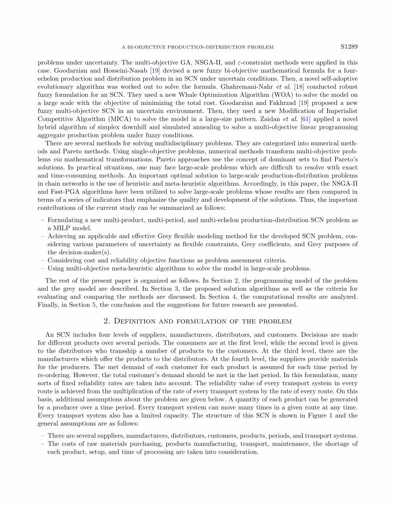
solutions. Here, for each solution xi in the population, a weak power value S(xi) is allocated, which indicatesthe number of the dominated solutions.

S (Xi) = |xj∀xj ∈ CPt ∧ xi > xj ∧ j 6= i| . (3.1)

The cardinal of a set is shown by |, |. CPt is the set of solutions for generation t, and the expression xi > xjmeans that the solution xi dominates solution xj . The merit value of each dominated solution is calculated bythe following equation:

F (xi) =∑xi>xj

S (xj)−∑xk>xi

S (xk) ∀xj · xk ∈ CPt ∧ j 6= i 6= k. (3.2)

In other words, the merit value of every dominated solution xi is equal to the difference between the sum ofthe power values of all the solutions that make up the dominated xi and the sum of the power values of all thesolutions that dominate xi. Practicing this approach involves only a few computations, because no mechanismis used; maintaining other varieties among non-dominated solutions needs few computations.

Once the merit values of all the population solutions are calculated and compared, three scenarios should benoted as follows:

(a) Two solutions are compared with different ranks. The solution to choose is the one with a better rank.(b) There are two equal-rank solutions, but there is a difference between the amounts of merit. In this case, the

solution to choose is the one with a higher merit value.(c) There are two solutions with the same rank and merit. In this case, one of them is chosen randomly.

3.2.2. Elitism and population adjustment

In this section, the population of the previous generation and that of the offspring are combined. This providesthe opportunity to maintain the superior solutions in the next generations and to ignore the weak ones. If thepopulation is too large and is constant over different generations, it leads to a reduction in elitism in theearly generations. Also, the existence of fluctuation in the number of non-dominated solutions over differentgenerations requires an adaptive population size strategy to emphasize the intensity of elitism in non-dominatedsolutions. If the intensity of elitism is very low, convergence may be too late. This imposes a high computationalcost. On the other hand, if the intensity of elitism is very high, early convergence may occur. Therefore, thisalgorithm dynamically uses a modifier operator to set the population size until it reaches a predetermined value.The modifier operator uses the following equation:

|Pt| = minat + [bt ∗ |xi|xi ∈ CPt ∧ xi is nondominated ·maxpopsize (3.3)

where |Pt| is the population size in generation t, αt and bt are the positive and the integer positive valuesrespectively, which may vary over different generations, xi is the smallest integer greater than or equal to thereal value of x, and maxpopsize represents the largest preset population size.

The Fast PGA algorithm, unlike many other evolutionary optimization methods, has the advantage of usingthe size of the offspring generated by crossover and mutation operators dynamically. The size of the offspringin each generation is calculated as follows:

|Ot| = minct + [dt ∗ |xi |xi ∈ CPt ∧ xi is nondominated ·maxsolved | (3.4)

where |Ot| is the size of the population of the offspring generated in generation t, ct and dt are the integerpositive and the true positive values respectively, and maxsolved represents the maximum number of theevaluated solutions in each generation. This dynamic Fast PGA algorithm allows the saving of a significantnumber of solutions at the beginning of the search and exploits extractions efficiently in later generations [33].


85762134

Figure 4. An example of how to represent the string of a chromosome.

85762134

86752314

86752134

85762314

Pc

Figure 5. An example of a uniform crossover process.

3.3. The used operators in the algorithm

3.3.1. How to display the solution?

This section presents several execution modes for each activity in the problem. Of these modes, only one isto be run. So, there is a need to display how a mode can be run for an activity. The most appropriate typeof display for the category of integer problems involves a chromosome as a set of integer values (genes) thatrepresent the selected execution mode for a given activity of a problem. Figure 4 displays a feasible solution (asa string of a chromosome) for a problem with eight activities.

3.3.2. Calculation of objective functions

This section is dedicated to the comparison of different solutions with one another and ranking of themaccording to the calculated values for the objective functions. In fact, as the dominance rule suggests, if noneof the cost functions is worse than the others and at least one of the objectives is better than the others, onesolution can be considered superior to another one.

3.3.3. Crossover operator

The crossover operator depends on the type of display, and, for different displays, different operators must bedefined. Here, according to the type of display, the uniform crossover is used. It is the crossover operator relatedto integer representations [33,33,46,50,62]. In a uniform crossover, sequences of random variables are generatedfrom the uniform distribution in [0, 1] multiplied by the number of chromosome genes. In each position, if thevalue is less than parameter Pc, the gene will be generated from the first parent; otherwise, it will be inheritedfrom the second parent. The second offspring is generated in an opposite process (Fig. 5).

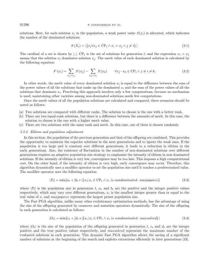
3.3.4. Mutation operator

Basically, the type of operator used for mutation depends on the type of presentation. In this case, we usethe random replacement operator, which is one of the common methods for numeric representations [33,50]. Inthis operator, first, a string of random numbers with the length of the number of genes in the interval [0, 1] isgenerated. In each position of the string, if the corresponding random number is lower than the mutation rate,a new value is randomly assigned to a set of allowable values in each position which serve to select and replacethe number of the genes in that position. Otherwise, the number of the genes remains unchanged. For moreexplanation, see Figure 6.


85762134

85213476

Pm

Figure 6. An example of a random replacement mutation.

3.3.5. Parent choice mechanism

In the general structure of the algorithm, there is a two-stage evolutionary cycle based on competition. Thestages include (a) selection of individuals to participate in reproduction (parent selection) and (b) selection ofindividuals for survival in the next generation (choice of survivors).

In the genetic algorithm, the individuals with higher levels of fitness are more likely to be parental than thosewith lower fitness. Here, a binary variable is applied for parent’s selection. In this type of choice, at each stage2, choices are given, and the best individual is selected among them as a parent in terms of fitness. This isrepeated until the intended number of parents is selected [50].

3.3.6. Primary population generation

In this section, each gene is formed by the assignment of a mode of execution to every activity. This modeis selected randomly from a set of possible execution modes. It is done to reach the primary population. Thepossible execution modes for an activity actually refer to a set of modes that have the necessary quality toperform that activity. Accordingly, before the production of the initial population, a preprocessor functionshould be used to identify the inefficient operating modes whose total weight of quality indices is lower thana certain limit. These modes should be avoided because they may disturb any stage of population generation.Therefore, all the generated solutions are always feasible solutions.

3.3.7. Computational analyses

In this section, the authors firstly generate the test problems for the presented model developed. Accordingto the two conflicting objectives, four evaluating metrics are presented to assess the quality of non-dominatedsolutions of the meta-heuristics. Finally, a set of sensitivity analyses is utilized to examine the validity of thepresented model developed. To the best of our knowledge and according to the novelty of the presented model,no existing study has treated a similar model in the literature. Then, the benchmarks existing in the literatureis not available for the model and an approach is needed to design the test problems. In order to evaluatethe efficiency of the presented algorithms, a number of standard examples are generated for the problem. Tentest problems including two classifications i.e. small: SP1–SP4, medium sizes: MP5–MP7, and large sizes: LP8–LP10 are presented. Table 1 introduces the sizes of problem instances. Table 2 presents the parameters of thegenerated examples.

3.4. Parameters setting

Meta-heuristic algorithms are very sensitive to their setting parameters, and a change in those parametershas a significant impact on the efficiency of the algorithms. The proposed algorithms are coded utilizing theMATLAB R2016b software. They are implemented in the computer system with the characteristics of the Corei5/6 GHz processor and the 6GB side-mounted memory. Table 3 shows the proposed values for each parameterrelated to the NSGA-II and Fast PGA algorithms. As it is noted in the table, n represents the activities relatedto each problem. Therefore, some experiments were conducted on problems 2 and 6 to survey parameter settingfor small-scale problems (i.e. problems 1–4), medium-scale (i.e. problems 5–7), and large-scale problems (i.e.problems 8–10). Tables 4 and 5 present the parameter setting values for two algorithms in which the value of


Table 1. The instances for test problem.

Classifications Instance s p k i r v t

Small SP1 1 1 2 2 2 2 1SP2 2 2 3 3 4 3 2SP3 3 4 4 5 6 4 4SP4 3 4 4 5 6 4 4

Medium LP5 6 8 8 8 10 8 9LP6 8 10 12 10 12 10 10LP7 10 12 14 12 14 12 12

Large LP8 12 14 16 14 16 12 12LP9 14 16 18 16 18 14 12LP10 18 20 22 20 24 16 12

Table 2. Parameters for generated examples.

Problem Number ofactivities

Numberof runmodes

Cost Reliability Number ofreliabilityindicators

Reliability ofeach indicatorin each runmode

The minimumtotal of reliabilityindicators in eachrun mode

1 7 [2,9] [15,70] [120,190] 2 [60,99] [60,75]2 9 [2,4] [10,50] [10,20] 5 [60,99] [60,75]3 15 [2,7] [10,200] [30,60] 2 [60,99] [60,75]4 21 [2,6] [50,400] [250,480] 3 [60,99] [60,75]5 31 [2,6] [150,450] [50,140] 4 [60,99] [60,75]6 40 [2,5] [100,160] [50,120] 4 [60,99] [60,75]7 50 [2,5] [30,120] [80,180] 3 [60,99] [60,75]8 60 [2,6] [150,450] [100,200] 5 [70,99] [60,75]9 80 [2,5] [200,550] [150,250] 6 [80,99] [60,75]10 100 [2,8] [300,650] [200,300] 8 [90,99] [60,75]

each parameter is fixed by keeping the other parameters in their lowest value. This is done based on the numberof the non-dominated points identified through a certain number of repetitions.

3.5. Algorithms validation

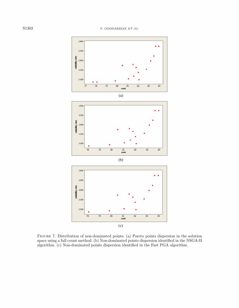
In order to prove that the results of the formulation fully reach the Pareto front side of the problem and thesolutions are necessary for dispersion, the efficiency of the methods used in the different parts of the algorithmsas well as the validity of the obtained solutions should be measured. Thus, three examples are generated on arelatively small scale. Then, through a search for all the possible spaces in these real-world problems, they areidentified and compared with the results of the algorithms. Table 6 presents the specifications of the examplegeneration, the results related to the full search of the solution space and their solutions through two algorithms.For instance, after a complete review of the solution space of an example, as in Table 7, it has been found thatthere are 15 non-dominated points for that example. As it can be seen, the obtained solutions have no superiorityto one another, and it is not possible to find a solution that is the best for all objects. The dispersion of thepoints in the solution space is indicated in Figure 7a. This problem has been obtained by NSGA-II and FastPGA algorithms in about four seconds to identify 14 and 13 non-dominated points respectively. Regarding theresults of the other two examples, it can be concluded that the validity and ability of the two algorithms to


Table 3. The initial value of proposed algorithms parameters.

Type of algorithm Parameter Proposed values

Mutation rate 0.1 0.2 0.3NSGA-II Intersection rate 0.4 0.5 0.6

Population numberof each generation

5n 7n 10n

a 2n 3n 4nb 0.5 1 1.5c 2n 3n 4nd 0 0.5 1Mutation rate 0.1 0.2 0.3

Fast PGA Intersection rate 0.4 0.5 0.6Maximum popula-tion

5n 7n 10n

Maximum numberof children

5n 7n 10n

Table 4. Parameter setting values for Fast PGA algorithm parameters.

The number of maximuma b c d Population of

offspringPopulation

Small-scale examples 4n 0.5 3n 0.5 5n 7nMedium-scale examples 3n 0.5 3n 1 5n 7nlarge-scale examples 5n 0.9 4n 1 6n 10n

Table 5. Parameter setting values for the parameters of the NSGA-II algorithm.

Mutation rate Intersection rate The population of each generation

Small-scale examples 0.2 0.4 6nMedium-scale examples 0.3 0.5 10nLarge-scale examples 0.8 0.6 12n

reach optimal solutions are acceptable. Figures 7b and 7c show the non-dominated points identified in the twoalgorithms.

3.6. The evaluating criteria and algorithms comparison

Through the comparison of two multi-objective algorithms in terms of efficiency, several useful indicators,or criteria, should be taken into account. These indicators are mainly divided into two categories. The firstemphasizes the convergence and the quality of the solutions, and the second emphasizes the dispersion and theexpansion of those solutions in the solution space. In this respect, there are four indicators for the comparisonof two algorithms [50]:

– Number of Pareto solutions (NPS),– Maximum spread or diversity (MS),– Mean ideal distance (MID),– Diversification metric (DM).


Table 6. Specifications and results related to the examples to validate algorithms.

Number of Number of Coefficient Total number of Total number of Total runtime The number of non- Runtime of two

activities modes complexity feasible points non-dominated points (second) dominated points which algorithms (seconds)

of solution space discovered by the algorithms

NSGA-II Fast PGA

8 [2,5] 1.43 4850 17 274 15 13 5

9 [2,5] 1.6 37 487 38 24 560 36 31 35

12 [2,4] 1.53 196 534 13 23 730 14 12 40

Table 7. The values of the objective functions related to non-dominated points of the firstexample.

Non-dominated points Reliability Cost

1 1275 83.962 1224 83.663 1163 83.484 1198 81.825 1137 83.186 1137 82.357 1179 81.588 1154 82.769 1118 81.5710 1104 81.0711 1174 80.5112 1099 82.0713 1093 79.8214 1087 78.0715 1087 77.71

4. Computational results

In this section, the examples generated in the previous section are solved with the NSGA-II and Fast PGAalgorithms. In order to assess and compare the two algorithms, the criteria mentioned in the previous sectionare used. Also, each example is run for 10 times by each algorithm, and the non-dominated solutions of these10 runs are used to compare the results. Therefore, the comparison of the algorithms is presented in small-scaleexamples (Examples 1–4), medium-scale examples (Examples 5–7), and large-scale examples (Examples 8–10).

4.1. Performance evaluation of proposed algorithms on small-scale problems

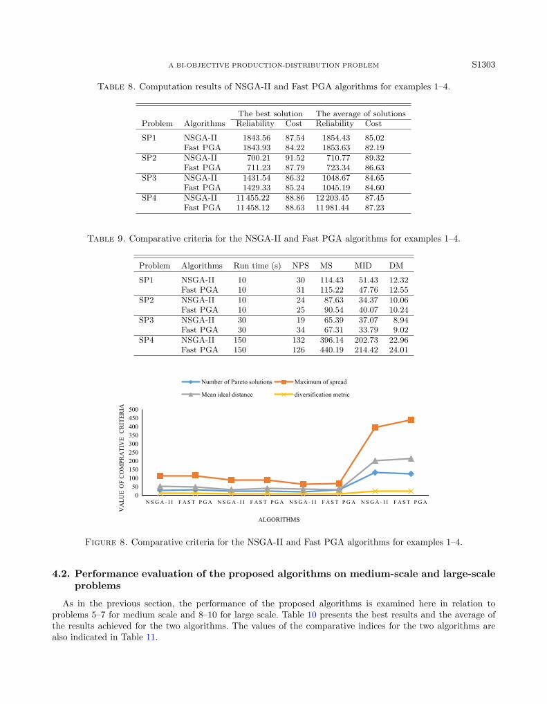
The performance and the efficiency of the NSGA-II and Fast PGA algorithms are compared in examples 1–4.In Table 8, the best results are executed in 10 times, and the average of the results obtained from this set ofruns is presented for the two algorithms. Also, Table 9 represents the values of the comparative indices for bothalgorithms. The run time is taken into consideration for two identical algorithms.

Table 9 and Figure 8 indicate that the Fast PGA algorithm is more successful than the NSGA-II algorithm infinding the number of Pareto’s points in all the problems, except problem 4. Regarding the mean distance fromthe ideal solution, there cannot be a decisive claim of superiority for one of the algorithms over the other. Formost of the expanding and diverse criteria that imply the dispersion and proper distribution of the solutions,the Fast PGA algorithm is significantly superior to NSGA-II.


(a)

(b)

(c)

Figure 7. Distribution of non-dominated points. (a) Pareto points dispersion in the solutionspace using a full count method. (b) Non-dominated points dispersion identified in the NSGA-IIalgorithm. (c) Non-dominated points dispersion identified in the Fast PGA algorithm.


Table 8. Computation results of NSGA-II and Fast PGA algorithms for examples 1–4.

The best solution The average of solutionsProblem Algorithms Reliability Cost Reliability Cost

SP1 NSGA-II 1843.56 87.54 1854.43 85.02Fast PGA 1843.93 84.22 1853.63 82.19



SP4 NSGA-II 11 455.22 88.86 12 203.45 87.45Fast PGA 11 458.12 88.63 11 981.44 87.23

Table 9. Comparative criteria for the NSGA-II and Fast PGA algorithms for examples 1–4.

Problem Algorithms Run time (s) NPS MS MID DM

SP1 NSGA-II 10 30 114.43 51.43 12.32Fast PGA 10 31 115.22 47.76 12.55




0

50

100

150

200

250

300

350

400

450

500

N S G A - I I F A S T P G A N S G A - I I F A S T P G A N S G A - I I F A S T P G A N S G A - I I F A S T P G A

VA

LU

E O

F C

OM

PR

AT

IVE

C

RIT

ER

IA

ALGORITHMS

Number of Pareto solutions Maximum of spread

Mean ideal distance diversification metric

Figure 8. Comparative criteria for the NSGA-II and Fast PGA algorithms for examples 1–4.

4.2. Performance evaluation of the proposed algorithms on medium-scale and large-scaleproblems

As in the previous section, the performance of the proposed algorithms is examined here in relation toproblems 5–7 for medium scale and 8–10 for large scale. Table 10 presents the best results and the average ofthe results achieved for the two algorithms. The values of the comparative indices for the two algorithms arealso indicated in Table 11.


Table 10. Computation results of NSGA-II and Fast PGA algorithms for examples 5–7 and 8–10.

The best solution The average of solutionsProblem Algorithms Reliability Cost Reliability Cost

MP5 NSGA-II 5349.71 87.54 5390.82 87.13Fast PGA 5408.52 87.33 5462.63 87.12

MP6 NSGA-II 8254.76 82.76 8342.46 82.65Fast PGA 8354.53 82.73 8403.28 82.66

MP7 NSGA-II 8434.62 85.94 11 477.33 85.32Fast PGA 9102.87 85.65 12 477.33 85.54

LP8 NSGA-II 9431.25 93.21 9567.12 92.76Fast PGA 9780.23 93.13 9877.38 92.53

LP9 NSGA-II 10 212.92 104.39 10 516.44 104.21Fast PGA 13 434.22 104.21 13 849.17 104.34

LP10 NSGA-II 14 555.67 156.83 16 772.12 155.67Fast PGA 18 939.26 156.67 19 566.59 155.29

Table 11. Comparative criteria for the NSGA-II and Fast PGA algorithms for examples 5–7and 8–10.

Problem Algorithms Run time (s) NPS MS MID DM

MP5 NSGA-II 600 52 354.51 158.09 20.05Fast PGA 600 49 566.84 183.76 23.49



LP8 NSGA-II 1000 128 788.55 201.21 28.45Fast PGA 1000 56 467.84 167.45 23.12



According to the results presented in Table 11 and Figures 9 and 10, it can be claimed that the NSGA-IIalgorithm yields better results with the number of non-dominated solutions, while the Fast PGA algorithmperforms better in terms of solution variety. As expected, if the size of the problem and the solution spaceof the NSGA-II algorithm are increased, compared with the Fast PGA, the number of Pareto’s points willbe found. This is due to the fast convergence of the Fast PGA algorithm to reach non-dominated points. Inthis algorithm, higher iterations lead to the generation of feasible optimal solutions. As it was observed, forsmall-scale examples, both algorithms have roughly equal performance, and the differences in their results canbe ignored. When the size of problems increases, however, the differences become more and more evident.

Of course, one cannot ignore the role of runtime in achieving the best solutions. Obviously, the higher theruntime, the better the NSGA-II algorithm functions than the other one. The shorter the runtime, however,the more favorable the Fast PGA algorithm is to the other one. Of course, as mentioned before, due to itshigh convergence, the Fast PGA algorithm is used in cases where the evaluation of the solutions is eithercomputational or financially cost-effective, or good solutions are to be found in a short time.


0

500

1000

1500

2000

2500

3000

N S G A - I I F A S T P G A N S G A - I I F A S T P G A N S G A - I I F A S T P G AVA

LU

E O

F C

OM

PR

AT

IVE

C

RIT

ER

IA

ALGORITHM




0

100

200

300

400

500

600

700

800

900

1000

N S G A - I I F A S T P G A N S G A - I I F A S T P G A N S G A - I I F A S T P G AVA

LU

E O

F C

OM

PR

AT

IVE

C

RIT

ER

IA

ALGORITHMS




Moreover, to find out the best meta-heuristic decisively, this study conducts a set of statistical comparisonsamong meta-heuristics based on Pareto optimal analyses taken by measurement metrics. Accordingly, the resultswhich were reported by Tables 8–11 are transformed into a well-known metric, namely, Relative Deviation Index(RDI) as the following formula [50]:

RDI =|Algsol − Bestsol|Maxsol −Minsol

× 100 (4.1)

where Algsol is the objective value obtained by a given measurement metric of algorithm, Maxsol and Minsolare respectively the maximum and the minimum values among all values outputted by algorithms. Bestsol isthe best solution among methods; in another word, it is one of the Maxsol and Minsol according to the natureof metrics [21]. It is evident that a lower value of RDI brings a higher quality of algorithms. Consequently, themeans plot and Least Significant Difference (LSD) for the proposed modified and hybrid algorithms and theirindividual ones have been resulted. The results run by Minitab 16 Statistical Software are shown in Figure 11.According to Figure 11, based on NPS, MID, MS, and DM metrics, the Fast PGA algorithm shows the bestperformance.


Figure 11. ANOVA plots for the assessment metrics in term of RDI FOR meta-heuristics(i.e. (a) for NPS, (b) for MID, (c) for MS and (d) for DM.)

4.3. Sensitivity analyses

This section contains the results of three tests applied to assess the sensitivity analysis of the impact of theparameters on the values of the decision variables and the objective function of the presented model. Sincethe Fast PGA algorithm proved to be the most effective one in the comparisons, we used it for this sensitivityanalysis, applied to the large-sized experimental problem LP6. The results of each test include the value of thetotal cost (TC) and the reliability (R).

The first experiment considers modifications in the parameter of the raw material cost (rpst). The secondexperiment focuses the parameter of the reliability ratio of transport system (rastssp, raj

tspk, radtski). We designed

four experiments for each parameter and analyzed the changes in the objective functions. The relevant resultsare presented in Tables 12 and 13, and the trade-off between objective functions of total cost and reliability arepresented as normalized values in Figures 12 and 13.

As indicated in Table 12 and Figure 11 with an increase in raw material cost, in the four experiments thevalue of the objective function increases slowly with TC and then R is fixed and without change. Additionally,by increasing reliability ratio of transport systems, the first objective function is remained fixed but the secondobjective function is raised according to the Table 13 and Figure 12.

4.4. Management insight

This study attempts to develop a new solution methodology in a supply chain network (SCN) design undergrey flexible condition. Hence, by optimizing the network configurations, managerial capabilities in elevating


Table 12. The results of the sensitivity analysis related to the first experiment.

The number of cases #rpst TC R

C1 10000 854.32 312.41C2 20000 945.34 312.41C3 30000 997.21 312.41C4 40000 1023.12 312.41

Table 13. The results of the sensitivity analysis related to the second experiment.

The number of cases #rastssp#rajts

pk#radtski TC R

C1 #10000#15000#20000 854.32 312.41C2 #15000#20000#25000 854.32 378.23C3 #25000#30000#35000 854.32 467.27C4 #35000#40000#45000 854.32 678.29

0

200

400

600

800

1000

1200

1 2 3 4

NO

RM

AL

IZE

D V

AL

UE

OF

OB

JE

CT

IVE

FU

NC

TIO

N

CASE NO.

TC R

Figure 12. The behavior of normalized objective functions for sensitivity analysis in the firstexperiment.

0

200

400

600

800

1000

1 2 3 4

NO

RM

AL

IZE

D V

AL

UE

OF

OB

JE

CT

IVE

FU

NC

TIO

NS

CASE NO.

TC R

Figure 13. The behavior of normalized objective functions for sensitivity analysis in the secondexperiment.

their SCN, and also solving real-world problems are improving. Such improvements can help many industries,e.g. the pharmaceutical and the car industries in applying theoretical developments for real cases. On the otherside, when managers decide to apply such models in their organization, problems result in most cases, whichgeneral exact solvers are unable to cope with. Additionally, the outcomes of the model have tremendous effectson management decisions for the production and distribution of the SCN. Therefore, elevating the capabilitiesof solving such vital problems and proposing new methodologies which can solve real cases inappropriate time


with reliable solutions, are important steps to the applicability of SCN problems in real situations for managersand industries. Therefore, the results of this paper present powerful and reliable methods for managers to copewith supply chain network design and planning issues. It also encourages managers to revise the production-distribution decisions of the SCN of their organizations.

5. Conclusion

In this paper, a novel multi-echelon, multi-objective, multi-product, and multi-period production-distributionmodel is developed in the SCN design problem. This model is based on two objective functions includingminimizing the operating costs of suppliers, manufacturers, distributors, and customers and maximizing thereliability of the system. The proposed model is formulated in the form of MILP. In the context of Grey flexiblelinear mathematical programming, the model deals with Grey/flexible constraints jointly; that is, the Greycoefficients for the lack of knowledge and the Grey purpose of the decision maker(s). Because the problembelongs to the category of NP-hard problems, and an increase in the problem size makes its solution timeincrease exponentially, the model makes use of the NSGA-II and Fast PGA algorithms, which are among thealgorithms used in multi-objective problems. After the corresponding parameters were set in this study, the twoalgorithms were compared in terms of several indices for several examples generated in different sizes. Finally,the computational results were analyzed for those examples.

In this study, all model parameters are considered as deterministic parameters. However, the proposed modelcould be extended to consider the uncertainty in demand, costs, and capacity for future work. Additionally, theperformance of the NSGA-II and Fast PGA can be compared with other meta-heuristic algorithms such as theTabu, particle swarm optimization, and social engineering optimization algorithms. In addition, other approachessuch as simulation-based optimization can be applied instead of a mathematical programming approach, whichcan lead to interesting findings. On the other hand, the bi-objective approach can be elevated to multi-objectiveapproaches, which let the network consider some essential objectives such as minimizing CO2 emissions andshortage of products and maximizing the number of customer respondents.

Appendix A. Related materials about grey system

A.1. Definitions, remarks, and theorems

Definition A.1. A grey system is defined as a system which includes uncertain information presented by greyvariables and grey numbers.

Definition A.2. Suppose X is a universal set. Here, X = R is considered as the set of all real numbers. Then,the grey system, G, of X is determined by the two maps µG and µG, where µG : X → [0, 1], µG : X →[0, 1]µG ≥ µG. The µG and µG are the lower and the upper membership functions in G respectively. The GreySystems (GS) theory introduces the concept of interval grey numbers. Grey numbers are considered as the basicunit of grey systems to apply in the formulation of a grey model. It can be a significant factor in the grey systemtheory [59]. Let X specify a bounded and closed set of real numbers.

Definition A.3. A grey number is a number with clear lower and upper boundaries, but it has an unknownposition within the boundaries. In the system, a grey number is represented mathematically as:

⊗x = [x¯, x] = t ∈ x|x

¯≤ t ≤ x (A.1)

where t is information,⊗x orxG is a grey number, x¯

and x are the lower and the upper limits of the characteristic [56].

Remark A.4. Note that the notations ⊗x and xG are the same grey number, and, for simplicity in modeling,the notation xG is sometimes applied for the mentioned grey number.

There are different kinds of grey numbers (see them in [2, 30–32, 39]). Among them, interval grey numbersare applied here as appropriate ones reported in the literature.


Definition A.5. An interval grey number is the one with both upper limit x and lower limit x¯

: ⊗ ∈ x[x¯, x].

Definition A.6 (White and black numbers). When ⊗ ∈ x(−∞,+∞), i.e., when ⊗x ∈ [x¯, x] and x

¯= x, ⊗x is

called a white number. When x has neither a lower limit nor an upper limit, the limits are all grey numbers; inthis case, ⊗x is called a black number.

The rest of the current study deals with interval grey numbers. For simplicity, they are briefly called greynumbers.

Remark A.7. For any real number a, if ⊗ = a[a, a], we say ⊗a is the corresponding grey number. In reality,any real number is a white number. Thus, without loss of generality, throughout the study, it can be ⊗ = 0[0, 0]as the zero grey number. For simplicity, it is shown with ⊗0 or 0.

Remark A.8. The set of all grey numbers is denoted by R(⊗) which can represent an element as ⊗x ∈ [x¯, x].

It belongs to (⊗) by ⊗x ∈ [x¯, x].

Definition A.9. Let L(⊗x) = |x− x¯| represent the length of the grey number ⊗x ∈ [x

¯, x]. It is clear that

L(⊗x) : R(⊗)→ R+ ∪ 0.Let two grey numbers be defined as ⊗x1 ∈ [x

¯1, x1] and ⊗x2 ∈ [x¯2, x2]. The arithmetic operations are defined

as follows:

⊗x1 +⊗x2 = [x¯1 + x

¯2, x1 + x2] (A.2)⊗x1 −⊗x2 = [x

¯1 − x¯2, x1 − x2]. (A.3)

The following theorems are quoted from Xie and Liu [59].

Theorem A.10. The result of the self-minus of a grey number is zero. That is, ⊗x−⊗x = 0.

Lemma A.11. If k ∈ R, ⊗x ∈ [x¯, x] is a grey number, we will have:

k · (⊗x) = ⊗(kx) ∈ [kx¯, kx] if k ≥ 0, (A.4)

k · (⊗x) = ⊗(kx) ∈ [kx, kx¯

] if k < 0. (A.5)

Definition A.12. The whitening number of a grey value, ⊗x, is determined as a deterministic number withits value lying between the lower and the upper bounds of ⊗x (see [58]):

x¯≤ ⊗x ≤ x

where ⊗x is the whitening value of ⊗x. This relationship can be represented as:

⊗x = x¯

+ α (x− x¯)

where the grey coefficient is specified by the α.

Theorem A.13. The set of all the grey numbers establishes a field.

Proof. It is straight forward as given in Shi et al. [52].

A.2. Ranking of grey numbers

There are several approaches to rank the grey numbers. Some of them are mentioned here.


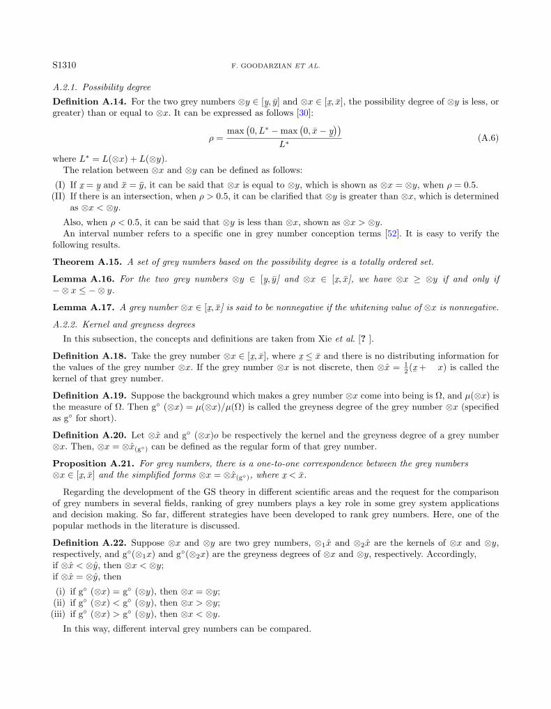
A.2.1. Possibility degree

Definition A.14. For the two grey numbers ⊗y ∈ [y¯, y] and ⊗x ∈ [x

¯, x], the possibility degree of ⊗y is less, or

greater) than or equal to ⊗x. It can be expressed as follows [30]:

ρ =max

(0, L∗ −max

(0, x− y

¯

))L∗

(A.6)

where L∗ = L(⊗x) + L(⊗y).The relation between ⊗x and ⊗y can be defined as follows:

(I) If x¯

= y¯

and x = y, it can be said that ⊗x is equal to ⊗y, which is shown as ⊗x = ⊗y, when ρ = 0.5.(II) If there is an intersection, when ρ > 0.5, it can be clarified that ⊗y is greater than ⊗x, which is determined

as ⊗x < ⊗y.

Also, when ρ < 0.5, it can be said that ⊗y is less than ⊗x, shown as ⊗x > ⊗y.An interval number refers to a specific one in grey number conception terms [52]. It is easy to verify the

following results.

Theorem A.15. A set of grey numbers based on the possibility degree is a totally ordered set.

Lemma A.16. For the two grey numbers ⊗y ∈ [y¯, y] and ⊗x ∈ [x

¯, x], we have ⊗x ≥ ⊗y if and only if

−⊗ x ≤ −⊗ y.

Lemma A.17. A grey number ⊗x ∈ [x¯, x] is said to be nonnegative if the whitening value of ⊗x is nonnegative.

A.2.2. Kernel and greyness degrees

In this subsection, the concepts and definitions are taken from Xie et al. [? ].

Definition A.18. Take the grey number ⊗x ∈ [x¯, x], where x

¯≤ x and there is no distributing information for

the values of the grey number ⊗x. If the grey number ⊗x is not discrete, then ⊗x = 12 (x

¯+ x) is called the

kernel of that grey number.

Definition A.19. Suppose the background which makes a grey number ⊗x come into being is Ω, and µ(⊗x) isthe measure of Ω. Then g (⊗x) = µ(⊗x)/µ(Ω) is called the greyness degree of the grey number ⊗x (specifiedas g for short).

Definition A.20. Let ⊗x and g (⊗x)o be respectively the kernel and the greyness degree of a grey number⊗x. Then, ⊗x = ⊗x(g) can be defined as the regular form of that grey number.

Proposition A.21. For grey numbers, there is a one-to-one correspondence between the grey numbers⊗x ∈ [x

¯, x] and the simplified forms ⊗x = ⊗x(g), where x

¯< x.

Regarding the development of the GS theory in different scientific areas and the request for the comparisonof grey numbers in several fields, ranking of grey numbers plays a key role in some grey system applicationsand decision making. So far, different strategies have been developed to rank grey numbers. Here, one of thepopular methods in the literature is discussed.

Definition A.22. Suppose ⊗x and ⊗y are two grey numbers, ⊗1x and ⊗2x are the kernels of ⊗x and ⊗y,respectively, and g(⊗1x) and g(⊗2x) are the greyness degrees of ⊗x and ⊗y, respectively. Accordingly,if ⊗x < ⊗y, then ⊗x < ⊗y;if ⊗x = ⊗y, then

(i) if g (⊗x) = g (⊗y), then ⊗x = ⊗y;(ii) if g (⊗x) < g (⊗y), then ⊗x > ⊗y;(iii) if g (⊗x) > g (⊗y), then ⊗x < ⊗y.

In this way, different interval grey numbers can be compared.


A.2.3. Ranking of grey numbers based on whitenization values

An appropriate method for solving GLP problems is to compare grey numbers in terms of the correspondingwhitenization values. An efficient method to order the elements of R(⊗) is to assign a whitenization value toevery grey number. The whitened function to xG : R(⊗)→ R maps each grey number in a genuine line, wherea natural order exists. In fact, for every ⊗x ∈ R(⊗), there is the relationship RG(⊗x) = ⊗x. Therefore, theorder of R(⊗) can be defined based on whitenizaion values as follows:

⊗x ≥ ⊗y if and only if ⊗x ≥ ⊗y;⊗x > ⊗y if and only if ⊗x > ⊗y;⊗x = ⊗y if and only if ⊗x = ⊗y;

where ⊗x and ⊗y belong to (⊗). Also, there is ⊗x ≤ ⊗y if and only if ⊗x ≥ ⊗y. By the above definition,⊗x > ⊗0 holds true when ⊗x ≥ 0. A corresponding lemma can be also described simply as follows.

Lemma A.23. Let xG be any whitened function. Then,

(i) ⊗x ≥ ⊗y if and only if ⊗x−⊗x ≥ ⊗0, and if and only if −⊗ y ≥ −⊗ x;(ii) If ⊗x ≥ ⊗y and ⊗u ≥ ⊗v, then ⊗x+⊗u ≥ ⊗y +⊗v;

where ⊗x, ⊗y, ⊗u, and ⊗v belong to (⊗) and ⊗0. The latter is a grey zero number which is defined inRemark A.8.

A.3. Grey flexible linear programming

An appropriate fuzzy linear programming model is the Grey Flexible Linear Programming (GFLP), whichpractically involves various formulations of flexible linear programming [5, 24]. In the following subsection, adefinition is given for this type of problems. Whatever discussion that follows is based on this definition.

A.3.1. GFLP problem with a linear membership function

Suppose a decision maker faces a linear programming problem in which s/he can endure violation in com-pleting the constraints; that is, s/he allows the constraints to be held as well as possible. When there is a setof constraints, the assumptions aix F bi and i = 1, . . . , n can be made for each constraint and formulated bythe use of a membership function as follows:

µi (x) =

1, aix ≤ bif (aix)i , bi ≤ aix ≤ bi + pi0, aix ≥ bi + pi

(A.7)

where fi(0) is continuous and strictly decreasing for aix, fi(bi) = 1 and fi(bi + pi) = 0.Equation (A.6) emphasizes that the decision maker can tolerate violation in the accomplishment of constraints

i up to the value bi + di. Considering the assumptions, the associated GFLP problem is represented as:

max zG(x) = cGx

s.t. Ax ≤F bx ≥ 0

or, (A.8)

max zG(x) = cGx

s.t. Hi(z, ai) =n∑j=1

aix− bi ≤F 0, i = 1, . . . ,m,

xj ≥ 0, j = 1, . . . , n,


where xT = (x1, x2, . . . , xn) is a n-dimensional real decision, and cG =(cG1 , c

G2 , . . . , c

Gn

)is a n-dimensional vector

of grey parameters involved in the grey objective Z. Also the notation “max” maximizes the objective functionin a fuzzy sense and “F” represents a fuzzy extension of “≤” on R which is applied to compare the left sideof fuzzy constraints with the right side.

In general, the main model is not well-defined due to the following reasons:

(i) The grey quantity z(cG, x) cannot be maximized based on the current method.(ii) The constraint Hi (x, ai) =

∑nj=1 aix− bi ≤F 0 does not result in a crisp feasible set.

An appropriate approach to state the crisp optimal solution preference of an alternative is comparing thegrey quantities using the whitenization function RG : R(⊗) → R that maps each grey quantity to a real linewhich exists a natural order (for more detail, refer to [9, 52]).

In addition, if a deterministic feasible set is to be specified, a confidence level αi should be provided sothat a desirable corresponding i-th fuzzy constraint can hold. Therefore, in order to remove those mentionedrestrictions, the following problem is introduced:

max z(x) = R(cG)x

s.t. µiHi (x, ai) ≤F 0 ≥

αi,

x ≥ 0, αi ≥D αDi, 0 ≤ αi ≤ 1, i = 1, . . . ,m, (A.9)

where z(x) = R(cG)x means the corresponding crisp value of grey function zG(x) based on linear rankingfunction. To choose a suitable membership function for each fuzzy constraint, it is argued that, if Hi(x, ai) ≤ 0,then the i-th constraint is fully met. However, if Hi(x, ai) ≥ pi, then the i-th constraint is perfectly violated.In the latter formula, pi is the predefined maximum tolerance from zero, as defined by the decision maker. ForHi(x, ai) ∈ (0, 1), it is recommended by Liu and Zhang [33] that the membership function of the i-th constraintbe applied as:

µ (Hi (x, ai) ≤ 0) =

1, Hi (x, ai) ≤ 01− Hi(x,ai)

pi, 0 ≤ Hi (x, ai) ≤ pi

0, Hi (x, ai) ≥ 0. (A.10)

And this is equal to:

µi(x) =

1, x, ai ≤ bibi+pi−aix

pi, bi ≤ aix ≤ bi + pi

0, aix ≥ bi + pi

. (A.11)

And the (3.1) gets:

max z(x) = R(cG)x

s.t. aix ≤ b+ pi (1− ai)x ≥ 0, αD

i≤ αi, 0 ≤ αi ≤ 1, i = 1, . . . ,m. (A.12)

The above problem is called Multi-Parametric Linear Programming problem (MPLP1).Now, a feasible solution is made to the grey linear programming problem as presented in (A.12).

Definition A.24. Let α = (α1, . . . , αm) ∈ (0, 1]m, then Xα = ∩mi=1 xiαi

, where

Xai =x ∈ <n

∣∣x ≥ 0, aix ≤ bi + pi (1− ai) , ai ≥ aDi, i = 1, . . . ,m. (A.13)

For i = 1, . . . ,m (namely, Xia is the α-cut of the i-th fuzzy constraint).

Proof. For any a = (a1, . . . , am) ∈ (0, 1]m , let x ∈ Xa. Therefore, ai ≥ aDi , aix ≤ bi+pi (1− ai). With regard toequation (3.4), we have x ∈ Xi

ai, i = 1, . . . ,m. Therefore, X ∈ ∩mi=1 x

iαi

. Also, If X ∈ ∩mi=1 xiαi

, we have x ∈ Xiai

,for all i = 1, . . . ,m. Therefore, ai ≥ aDi , aix ≤ bi + pi (1− ai) and hence x ∈ Xa. This completes the proof.


Proposition A.25. Let α′ = (α′1, . . . , α′m) and α′′ = (α′′1 , . . . , α

′′m), where α′i ≤ α′′i holds for all i, then α′′-

feasibility of x implies the α′-feasibility.

Proof. The proof is straightforward.

For a given α ∈ (0, 1], let x ∈ R be a usual α-feasible solution to (A.10). It is to be noted that this solutionprovides the same degree of satisfaction for all the constraints. It has the meaning of aix ≤ bi+pi (1− αi) , αi ≥ αDior equivalently x ∈ Xi

a, for all i =1,. . . ,m.If α = (α, . . . , α), then x ∈ Xα which implies that the α-feasibility of (A.10) can be understood as a special

case of the α-feasibility. Thus, the following result can be obtained.

Remark A.26. If the problem (A.10) is not infeasible, then Xα is not empty.

Proof. The proof is straightforward.

Definition A.27. Let “≺F ” be a fuzzy extension of binary relation “≤” and let x = (x1, . . . , xn)T ∈ <n bean α-feasibility solution to (A.10), where α = (α1, . . . , αm) ∈ (0, 1]m. Also, let cGx be a grey objective. Thevector nx ∈R is an α-efficient solution to (A.10) with maximization of the objective. In this case, if there is nox′ ∈ Xα, the relation cGx < cGx′ holds true.

Similarly, an α-efficient solution with the optimization of the objective can be defined.It is to be noted that any α-efficient solution to the GFLP problem is an α-feasible solution to that problem

with some extra properties. In the following theorem, a necessary and sufficient condition is postulated for aα-efficient solution to (3.3).

Theorem A.28. Let α = (α1, . . . , αm) ∈ (0, 1]m and x∗ = (x∗1, . . . , x∗n)T , x∗j ≥ 0, j = 1, . . . , n be a α-feasible

solution to (A.10). Then, the vector x∗ ∈ <n is an α-efficient solution to the problem (A.10) with the optimiza-tion of the objective if and only if x∗ is optimal in the following mathematical model:

max z (x) = R(cG)x

s.t. aix ≤ bi + pi (1− ai)x ≥ 0, αDi ≤ αi, 0 ≤ αi ≤ 1, i = 1, . . . ,m (A.14)

where pi is the predefined maximum tolerance.

Proof. Let α = (α1, . . . , αm) ∈ (0, 1]m and x∗ = (x∗1, . . . , x∗n) , x∗j ≥ 0, j = 1, . . . , n be an α-feasible

solution to (A.11) with optimization of the objective. By “Definition A.24” and equation (A.10), we haveaix∗ ≤ bi + pi (1− αi) , αi ≥ αD

ifor i =1,. . . , m. Therefore, x∗ is a feasible solution to (A.12). In this case, x∗

is obviously an α-feasible solution to problem (A.11). Thus, by “Definition A.27”, the optimality of x impliesthe α-efficiency of x∗.

In Theorem A.28, we have provided a computational method to solve fuzzy flexible linear programming prob-lem (A.11). Thus, when a specific α is assigned by a decision maker, the αj can be replaced in the correspondingconstraint of (A.12), and the resulted problem can be solved. An α-efficient solution is, thus, made to problem(A.11). Such a solution has two characteristics:

(i) It provides various satisfaction degrees depending on the constraints.(ii) It is an optimal solution.

This solution permits decision makers to achieve more flexibility and compatibility by assigning desiredpreferences, especially in online optimization for more desirable cases.

In Theorem A.28, a method is introduced to obtain an α-efficient solution to a GELP problem. If the resultingproblem (A.12) has only one optimal solution, the theorem is confirmed. This solution is, thus, an α-efficient


one for a given fuzzy problem. In this case, problem (A.12) has some multiple optimal solutions. In order tofind a maximum efficient solution, i.e., an α′-efficient solution with α′ ≥ α, i = 1, . . . ,m, a two-phase approachis applied as follows. In Phase (I), problem (A.12) is solved. In Phase (II), a solution is obtained with a highersatisfaction degree than the previous one. So by the use of a two-phase approach, the available resources canbe utilized better. Also, the solution resulting by this two-phase approach is always an α′-efficient solution.

Problem (A.12) is called a “Phase (I) problem”. Let α0 =(α0

1, . . . , α0m

)and

(x∗, z

(cG, x∗

))be the optimal

solution of Phase (I) with the α0 degree of efficiency. Set α∗i = µiHi (x∗, αi) ≺F 0

≥ α0

i . In Phase (II), thefollowing problem is solved as follows:

max Wα =m∑i=1

αi

R(cG)x ≥ R

(cG)x∗

aix ≤ bi + pi (1− ai)s.t. 0 ≤ αi ≤ 1, α∗

i≤ αi, i = 1, . . . ,m

x ≥ 0. (A.15)

The above problem is named a Multi-Parametric Linear Programming (MPLP) problem. Let(x∗∗, α∗∗1 , . . . , α∗∗m ) be an optimal solution to problem (A.15), i.e. (MPLP). Then, we have the following theorem.

Theorem A.29. In the optimal solution x∗∗ to the problem (A.15), or (MPLP), x∗∗ is a maximum α-efficientsolution to the problem (A.11).

Proof. In problem (A.15), there is the relationship α∗i ≥ α0i . Therefore, using Proposition A.25, x∗∗ is an

α-feasible solution to problem (A.12). This implies that it is feasible in problem [42]. Now, by the optimal-ity of x∗ in problem (A.9) and z(x∗) = cGx∗ ≤ z(x∗∗) = cGx∗∗, there is the optimality of x∗∗ in problem[43]; hence, z(x∗) = cGx∗ = z(x∗∗) = cGx∗∗. This means that x∗∗ is also an α0-efficient solution to prob-lem (A.14). Because (x∗∗, α∗∗1 , . . . , α∗∗m ) is optimal and the coefficients in the objective function of problem(A.15) are positive, we have α∗∗i = µi

Hi (x∗, αi) ≺F 0

, i = 1, . . . ,m. Now, if possible, let x∗∗ be not a max-

imum α0-efficient solution to problem (33). Then, there exists an α0-efficient x′ to problem (A.14) such thatα′i > α∗∗i , i = 1, . . . ,m and for some k, α′k > α∗∗k . In this case, α′i = µi

Hi (x, ai) ≺F 0

, i = 1, . . . ,m and

z (x′) = cGx′ ≥ z (x∗) = cGx∗. Therefore, (x′, α′1, . . . , α′m) serves as a feasible solution to problem (A.15) and∑m

i=1 α∗∗i =

∑mi=1,i6=k α

∗∗i + α∗∗k <

∑mi=1,i6=k α

′i + α′k =

∑mi=1 α

′i.

But this implies that (x∗∗, α∗∗1 , . . . , α∗∗m ) is not a solution to problem (A.15), which is a clear contradiction.

The following section of the study is dedicated to the main steps of a desired method to solve a GFLPproblem based on the above theoretical discussions.

References

[1] O. Abdolazimi, M.S. Esfandarani, M. Salehi and D. Shishebori, Robust design of a multi-objective closed-loop supply chainby integrating on-time delivery, cost, and environmental aspects, case study of a Tire Factory. J. Cleaner Prod. 264 (2020)121566.

[2] M. Al Hail, W. Elkassem, A. Hamad, P. Abdulrouf, B. Thomas and D. Stewart, Overview of pharmacovigilance practices atthe largest academic healthcare system in the State of Qatar. Int. J. Clin. Pharm. 40 (2018) 769–774.

[3] M.H. Alavidoost, M. Tarimoradi and M.F. Zarandi, Bi-objective mixed-integer nonlinear programming for multi-commoditytri-echelon supply chain networks. J. Intell. Manuf. 29 (2018) 809–826.

[4] Z. Asim, S.A. Jalil and S. Javaid, An uncertain model for integrated production-transportation closed-loop supply chainnetwork with cost reliability. Sustainable Prod. Consumption 17 (2019) 298–310.

[5] H. Attari and S.H. Nasseri, New concepts of feasibility and efficiency of solutions in fuzzy mathematical programming problems.Fuzzy Inf. Eng. 6 (2014) 203–221.

[6] G.K. Badhotiya, G. Soni and M.L. Mittal, Fuzzy multi-objective optimization for multi-site integrated production and distri-bution planning in two echelon supply chain. Int. J. Adv. Manuf. Technol. 102 (2019) 635–645.


[7] M.M. Billal and M. Hossain, Multi-Objective optimization for multi-product multi-period four Echelon supply chain problemsunder uncertainty. J. Optim. Ind. Eng. 13 (2020) 1–17.

[8] Y. Cardona-Valdes, A. Alvarez and J. Pacheco, Meta-heuristic procedure for a bi-objective supply chain design problem withuncertainty. Transp. Res. Part B: Method. 60 (2014) 66–84.

[9] D. Darvishi, S. Liu and S.H. Nasseri, A new approach in animal diet using grey system theory. Grey Syst.: Theory App. 8(2018) 167–180.

[10] A.K. Das and D.K. Pratihar, A novel approach for neuro-fuzzy system-based multi-objective optimization to capture inherentfuzziness in engineering processes. Knowl.-Based Syst. 175 (2019) 1–11.

[11] A. Diabat, A. Jabbarzadeh and A. Khosrojerdi, A perishable product supply chain network design problem with reliabilityand disruption considerations. Int. J. Prod. Econ. 212 (2019) 125–138.

[12] M.B. Fakhrzad and F. Goodarzian, A fuzzy multi-objective programming approach to develop a green closed-loop supply chainnetwork design problem under uncertainty: modifications of imperialist competitive algorithm. RAIRO:OR 53 (2019) 963–990.

[13] M.B. Fakhrzad, P. Talebzadeh and F. Goodarzian, Mathematical formulation and solving of green closed-loop supply chainplanning problem with production, distribution and transportation reliability. Int. J. Eng. 31 (2018) 2059–2067.

[14] M.B. Fakhrzad, F. Goodarzian and A.M. Golmohammadi, Addressing a fixed charge transportation problem with multi-routeand different capacities by novel hybrid meta-heuristics. J. Ind. Syst. Eng. 12 (2019) 167–184.

[15] A.M. Fathollahi-Fard, A. Ahmadi, F. Goodarzian and N. Cheikhrouhou, A bi-objective home healthcare routing and schedulingproblem considering patients’ satisfaction in a fuzzy environment. Appl. Soft Comput. (2020) 106385.

[16] C. Feng, Y. Ma, G. Zhou and T. Ni, Stackelberg game optimization for integrated production-distribution-construction systemin construction supply chain. Knowl.-Based Syst. 157 (2018) 52–67.

[17] T. Gal, Post Optimal Analysis: Parametric Programming and Related Topics. De Gruyter, New York, NY (1994).

[18] J. Ghahremani-Nahr, R. Kian and E. Sabet, A robust fuzzy mathematical programming model for the closed-loop supply chainnetwork design and a whale optimization solution algorithm. Expert Syst. App. 116 (2019) 454–471.

[19] F. Goodarzian and H. Hosseini-Nasab, Applying a fuzzy multi-objective model for a production-distribution network designproblem by using a novel self-adoptive evolutionary algorithm. To appear in: Int. J. Syst. Sci.: Oper. Logistics (2019)DOI: 10.1080/23302674.2019.1607621.

[20] F. Goodarzian, H. Hosseini Nasab and M.B. Fakhrzad, A multi-objective sustainable medicine supply chain network designusing a novel hybrid multi-objective metaheuristic algorithm. Int. J. Eng. 33 (2020) 1986–1995.

[21] F. Goodarzian, H. Hosseini-Nasab, J. Munuzuri and M.B. Fakhrzad, A multi-objective pharmaceutical supply chain networkbased on a robust fuzzy model: a comparison of meta-heuristics. Appl. Soft Comput. 92 (2020) 106331.

[22] S. Jalali, M. Seifbarghy, J. Sadeghi and S. Ahmadi, Optimizing a bi-objective reliable facility location problem with adaptedstochastic measures using tuned-parameter multi-objective algorithms. Knowl.-Based Syst. 95 (2016) 45–57.

[23] S.F. Ji, X.S. Peng and R.J. Luo, An integrated model for the production-inventory-distribution problem in the PhysicalInternet. Int. J. Prod. Res. 57 (2019) 1000–1017.

[24] S. Karmakar and P. Mujumdar, Grey fuzzy optimization model for water quality management of a river system. Adv. WaterResour. 29 (2006) 1088–1105.

[25] S. Khalifehzadeh and M.B. Fakhrzad, A modified firefly algorithm for optimizing a multi stage supply chain network withstochastic demand and fuzzy production capacity. Comput. Ind. Eng. 133 (2019) 42–56.

[26] S. Khalifehzadeh, M. Seifbarghy and B. Naderi, Solving a fuzzy multi objective model of a production–distribution systemusing meta-heuristic based approaches. J. Intell. Manuf. 28 (2017) 95–109.

[27] A. Khanna, A. Kishore, B. Sarkar and C.K. Jaggi, Inventory and pricing decisions for imperfect quality items with inspectionerrors, sales returns, and partial backorders under inflation. RAIRO:OR 54 (2020) 287–306.

[28] J. Li, X. Zeng, C. Liu and X. Zhou, A parallel Lagrange algorithm for order acceptance and scheduling in cluster supplychains. Knowl.-Based Syst. 143 (2018) 271–283.

[29] S. Liu and L.G. Papageorgiou, Multi objective optimization of production, distribution and capacity planning of global supplychains in the process industry. Omega 41 (2013) 369–382.

[30] S.F. Liu and Y. Lin, Grey Information, Theory and Practical Applications, 1st edition. Springer, London (2006).

[31] S.F. Liu and Y. Lin, Grey Systems: Theory and Applications. Springer-Verlag, Berlin- Heidelberg (2011).

[32] S.F. Liu and N. Xie, Grey Systems Theory and its Applications. The Science Press of China, Beijing (2013).

[33] X. Liu and D. Zhang, An Improved SPEA2 algorithm with local search for multi-objective investment decision-making. Appl.Sci. 9 (2019) 1675.

[34] Y. Liu, H. Qin, L. Mo, Y. Wang, D. Chen, S. Pang and X. Yin, Hierarchical flood operation rules optimization using multi-objective cultured evolutionary algorithm based on decomposition. Water Resour. Manage. 33 (2019) 337–354.

[35] Z. Liu, S. Qu, M. Goh, R. Huang and S. Wang, Optimization of fuzzy demand distribution supply chain using modifiedsequence quadratic programming approach. J. Intell. Fuzzy Syst. 36 (2019) 6167–6180.

[36] Q. Long, A multi-methodological collaborative simulation for inter-organizational supply chain networks. Knowl.-BasedSyst. 96 (2016) 84–95.

[37] A. Megahed and M. Goetschalckx, A modeling framework and local search solution methodology for a production-distributionproblem with supplier selection and time-aggregated quantity discounts. Appl. Math. Model. 68 (2019) 198–218.

[38] M.R. Mohamadi, M. Abedini and B. Rashidi, An adaptive multi-objective optimization method for optimum design of distri-bution networks. Eng. Optim. 52 (2020) 194–217.

https://doi.org/10.1080/23302674.2019.1607621


[39] R.E. Moore, R.B. Kearfott and M.J. Cloud, Introduction to Interval Analysis. SIAM Press, Philadelphia, PA (2009).

[40] B. Naderi, K. Govindan and H. Soleimani, A Benders decomposition approach for a real case supply chain network designwith capacity acquisition and transporter planning: wheat distribution network. Ann. Oper. Res. 291 (2020) 685-705.

[41] S.H. Nasseri and S. Bavandi, Amelioration of Verdegay’s approach for fuzzy linear programs with stochastic parameters, Iran.J. Manage. Stud. (IJMS) 11 (2018) 71–89.

[42] S.H. Nasseri and D. Darvishi, Diet modeling in uncertainty conditions using Grey Systems approach. J. Oper. Res. App. 12(2016) 29–45.

[43] S.H. Nasseri and D. Darvishi, Duality results on grey linear programming problems. J. Grey Syst. 30 (2018) 127–142.

[44] M. Nazim, M. Hashim and J. Xu, Multi objective optimization of production-distribution problem under fuzzy random envi-ronment. Global J. Technol. Optim. 5 (2014) 161.

[45] R. Nourifar, I. Mahdavi, N. Mahdavi-Amiri and M.M. Paydar, Optimizing decentralized production–distribution planningproblem in a multi-period supply chain network under uncertainty. J. Ind. Eng. Int. 14 (2018) 367–382.

[46] M. Rabbani, R. Heidari and R. Yazdanparast, A stochastic multi-period industrial hazardous waste location-routing problem:Integrating NSGA-II and Monte Carlo simulation. Eur. J. Oper. Res. 272 (2019) 945–961.

[47] H. Rafiei, F. Safaei and M. Rabbani, Integrated production-distribution planning problem in a competition-based four-echelonsupply chain. Comput. Ind. Eng. 119 (2018) 85–99.

[48] Z. Rafie-Majd, S.H.R. Pasandideh and B. Naderi, Modelling and solving the integrated inventory-location-routing problem ina multi-period and multi-perishable product supply chain with uncertainty: Lagrangian relaxation algorithm. Comput. Chem.Eng. 109 (2018) 9–22.

[49] S.J. Sadjadi and A. Alirezaee, Impact of pricing structure on supply chain coordination with cooperative advertis-ing. RAIRO:OR 54 (2020) 1613–1619.

[50] N. Sahebjamnia, F. Goodarzian and M. Hajiaghaei-Keshteli, Optimization of multi-period three-echelon citrussupply chainproblem. J. Optim. Ind. Eng. (2020) 41–50.

[51] U. Sakalli and I. Atabas, Ant colony optimization and genetic algorithm for fuzzy stochastic production-distribution plan-ning. Appl. Sci. 8 (2018) 2042.

[52] J.R. Shi, S.Y. Liu and W.T. Xiong, A new solution for interval number linear programming. J. Syst. Eng. Theory Pract. 2(2005) 101–106.

[53] D. Shishebori and A. Ghaderi, An integrated approach for reliable facility location/network design problem with link disrup-tion. Int. J. Supply Oper. Manage. 2 (2015) 640–661.

[54] D. Shishebori and M.S. Jabalameli, A new integrated mathematical model for optimizing facility location and network designpolicies with facility disruptions. Life Sci. J. 10 (2013) 1896–1906.

[55] D. Shishebori, A.Y. Babadi and Z. Noormohammadzadeh, A Lagrangian relaxation approach to fuzzy robust multi-objectivefacility location network design problem. Sci. Iran. Trans. E Ind. Eng. 25 (2018) 1750–1767.

[56] W. Wang, Study on grey linear programming. J. Grey Syst. 9 (1997) 41–46.

[57] Z.X. Wang, Correlation analysis of sequences with interval grey numbers based on the kernel and greyness degree. Kybernetes42 (2013) 309–317.

[58] N.M. Xie, On computational algorithms of grey numbers based on information background. Grey Syst.: Theory App. 3 (2013)177–190.

[59] N.M. Xie and S.F. Liu, A novel grey relational model based on grey number sequences. Grey Syst.: Theory App. 1 (2011)117–128.

[60] X. Yan and Z. Song, The portfolio models of contained grey profit under uncertainty. Grey Syst.: Theory App. 4 (2014)487–494.

[61] A.A. Zaidan, B. Atiya, M.A. Bakar and B.B. Zaidan, A new hybrid algorithm of simulated annealing and simplex downhill forsolving multiple-objective aggregate production planning on fuzzy environment. Neural Comput. App. 31 (2019) 1823–1834.

[62] K. Zhang, Y. Cai, S. Fu and H. Zhang, Multi objective memetic algorithm based on adaptive local search chains for vehiclerouting problem with time windows. To appear in: Evol. Intell. (2019) DOI: 10.1007/s12065-019-00224-7.

[63] X. Zhao and J. Dou, Bi-objective integrated supply chain design with transportation choices: a multi-objective particle swarmoptimization. J. Ind. Manage. Optim. 15 (2019) 1263–1288.

https://doi.org/10.1007/s12065-019-00224-7

A bi-objective production-distribution problem in a supply ...

Documents

Transcript of A bi-objective production-distribution problem in a supply ...