
A Better Steam Engine: Designing a Distributed Concentrating … · A Better Steam Engine:...
125
A Better Steam Engine: Designing a Distributed Concentrating Solar Combined Heat and Power System By Zachary Mills Norwood A dissertation submitted in partial satisfaction of the requirements for the degree of Doctor of Philosophy in Energy and Resources in the Graduate Division of the University of California, Berkeley Committee in charge: Professor Daniel Kammen, Chair Professor Robert Dibble Professor Duncan Callaway Spring 2011
Transcript of A Better Steam Engine: Designing a Distributed Concentrating … · A Better Steam Engine:...
A Better Steam Engine:Designing a Distributed Concentrating Solar Combined Heat and Power System
By
Zachary Mills Norwood
A dissertation submitted in partial satisfaction of the
requirements for the degree of
Doctor of Philosophy
in
Energy and Resources
in the
Graduate Division
of the
University of California, Berkeley
Committee in charge:
Professor Daniel Kammen, ChairProfessor Robert Dibble
Professor Duncan Callaway
Spring 2011

Abstract
A Better Steam Engine:Designing a Distributed Concentrating Solar Combined Heat and Power System
by
Zachary Mills Norwood
Doctor of Philosophy in the Energy and Resources Group
University of California, Berkeley
Professor Daniel Kammen, Chair
The result of several years of analysis of Distributed Concentrating Solar Combined Heat andPower (DCS-CHP) systems is a design that is predicted to convert sunlight to heat at 8-10%solar-electric efficiency while simultaneously capturing ~60% of that initial sunlight as usableheat (at 100ºC). In contrast to similarly sized photovoltaic systems in the U.S. that cost~$7.90/Watt (Wiser et al. [44]) of generator rated peak electrical output, in mass production theproposed collector and generator system sized at 1-10kW would cost ~$3.20/Watt electricity and~$0.40/Watt-thermal, allowing adjustment of heat and electrical output on demand. The proposedsystem would revolutionize distributed energy generation in several ways: 1) by enabling rapiddissemination via avoidance of production limitations of photovoltaics such as expensive andlimited materials, 2) by efficient local production of both heat and power to offset moregreenhouse gases at a lower cost than other renewable energy technologies, and 3) bydemocratizing the means of electricity production; putting the power in the hands of the consumerinstead of large utilities. With over 5.4 GW of photovoltaics added globally in 2008 and 20GW ofsolar thermal (REN21 [29]), there is a large proven market for solar energy. With widespreadmarket penetration, this system would reduce greenhouse gas and criteria pollutant emissionsfrom electricity generation and heating for a significant portion of the developed and developingworld, including those in remote locations with no connection to an electric grid.
Chapter 1 begins with analysis of the relative demand for electricity and heat in California,showing that, on average, demand matches production of a theoretical solar CHP system. Then,we explore the economic and technological impetus for a solar powered combined heat and powerRankine cycle, showing cost and performance modeling in comparison to photovoltaics across
1

varying conditions, and concluding that solar CHP generated electricity is comparable to PVelectricity in terms of cost “per peak watt”. Chapter 2 shows results of a life cycle analysis ofDCS-CHP in comparison to other renewable and non-renewable energy systems including itsglobal warming potential (80 gCO2eq/kWh electric and 10 gCO2eq/kWh thermal), levelizedelectric and thermal energy cost ($0.25/kWh electric and $0.03/kWh thermal), and cost of solarwater purification/desalination ($1.40/m3). Additionally the utilization of water for thistechnology is shown to be much less than fossil-fuel based thermal power plants. Chapter 3explores the expander as an enabling technology for small solar Rankine cycles and presentsresults of physical testing and characterization of a rotary lobe expander prototype developed by asmall Australian company, Katrix, Inc. Testing of this expander using compressed air yields animpressive isentropic efficiency of 80-95% at pressure ratios of 6-11 making the rotary lobeexpander a leading choice for DCS-CHP systems, if operation on steam is successful andreliability issues can be addressed.
Chapter 4 concludes with a description and analysis of a DCS-CHP system using simulationsoftware developed in Matlab for the purpose of system analysis and optimization. This chapterfocuses on the selection of an appropriate expander and collectors, the two key enablingtechnologies for DCS-CHP. In addition to discussion of the rotary lobe expander, we present anovel collector device appropriate for solar CHP systems that eliminates high pressure articulatejoints, a typical failure point of solar concentrating systems. Given the results of the rotary lobeexpander testing, comparison to previous expander modeling work, and comparison of thepredicted cost and efficiency of the collectors analyzed, an appropriate technology version of theDCS-CHP system is selected and overall system performance is predicted across 1020 sites in theUS.
Keywords: solar · CHP · Rankine · CSP · concentrating · distributed · LCA · desalination.
2

To my family and friends.
i
Contents
1 Preliminary Performance, Cost, and Demand Analysis of Solar Combined Heat andPower Systems 11.1 Background . . . . . . . . . . . . . . . . . . . . . . . . . . . . . . . . . . . . . . 2
1.2 Solar Rankine thermodynamics matches California demand . . . . . . . . . . . . . 6
1.3 Performance-Cost analysis of solar combined heat and power systems . . . . . . . 8
1.4 Verification of the model for comparison to PV . . . . . . . . . . . . . . . . . . . 17
1.5 Discussion and conclusions . . . . . . . . . . . . . . . . . . . . . . . . . . . . . . 25
2 Life Cycle Analysis: Economics, Global Warming Potential, and Water for DistributedConcentrating Solar Combined Heat and Power 272.1 Introduction . . . . . . . . . . . . . . . . . . . . . . . . . . . . . . . . . . . . . . 28
2.2 Life Cycle Assessment of a single solar dish collector DCS-CHP system . . . . . . 28
2.3 Water and solar energy . . . . . . . . . . . . . . . . . . . . . . . . . . . . . . . . 31
2.4 Conclusions . . . . . . . . . . . . . . . . . . . . . . . . . . . . . . . . . . . . . . 42
3 Testing of the Katrix Rotary Lobe Expander 443.1 Introduction . . . . . . . . . . . . . . . . . . . . . . . . . . . . . . . . . . . . . . 45
3.2 Test setup for a Katrix rotary lobe expander . . . . . . . . . . . . . . . . . . . . . 47
3.3 Harmonic analysis, regulations for distributed generation . . . . . . . . . . . . . . 50
3.4 Results of the Katrix expander testing . . . . . . . . . . . . . . . . . . . . . . . . 52
3.5 Conclusions . . . . . . . . . . . . . . . . . . . . . . . . . . . . . . . . . . . . . . 63
4 Simulation Framework for a Distributed Concentrating Solar Combined Heat andPower System 644.1 Introduction . . . . . . . . . . . . . . . . . . . . . . . . . . . . . . . . . . . . . . 64
4.2 Program description . . . . . . . . . . . . . . . . . . . . . . . . . . . . . . . . . . 65
ii
4.3 Program structure . . . . . . . . . . . . . . . . . . . . . . . . . . . . . . . . . . . 67
4.4 Operation of the simulation software . . . . . . . . . . . . . . . . . . . . . . . . . 72
4.5 Case study of an appropriate DCS-CHP system . . . . . . . . . . . . . . . . . . . 75
4.6 Potential impact . . . . . . . . . . . . . . . . . . . . . . . . . . . . . . . . . . . . 85
5 Appendix A: Katrix Testing Equipment and Data 92
5.1 Test equipment . . . . . . . . . . . . . . . . . . . . . . . . . . . . . . . . . . . . 93
5.2 Katrix measured data from test runs . . . . . . . . . . . . . . . . . . . . . . . . . 93
6 Appendix B: Matlab Code for Katrix Data Processing 102
6.1 katrixDataProcess.m . . . . . . . . . . . . . . . . . . . . . . . . . . . . . . . . . 103
6.2 readxlsData.m . . . . . . . . . . . . . . . . . . . . . . . . . . . . . . . . . . . . . 106
6.3 orificeKatrixEfficiency.m . . . . . . . . . . . . . . . . . . . . . . . . . . . . . . . 108
6.4 Blevins.m . . . . . . . . . . . . . . . . . . . . . . . . . . . . . . . . . . . . . . . 110
6.5 rotameterKatrixEfficiency.m . . . . . . . . . . . . . . . . . . . . . . . . . . . . . 112
6.6 dpTorquePlot.m . . . . . . . . . . . . . . . . . . . . . . . . . . . . . . . . . . . . 112
iii
List of Figures
1.1 A typical wet steam Rankine cycle on a temperature-entropy diagram . . . . . . . 5
1.2 Rankine cycle for DCS-CHP modeled in EES . . . . . . . . . . . . . . . . . . . . 6
1.3 Average California residential daily demand compared with the solar Rankine sys-tem’s expected output of electricity (using R123 working fluid). (Norwood et al.[21]) . . . . . . . . . . . . . . . . . . . . . . . . . . . . . . . . . . . . . . . . . . 7
1.4 Distribution of collector costs; shaded regions represent power generation costs . . 11
1.5 Heat-only and CHP system diagrams . . . . . . . . . . . . . . . . . . . . . . . . . 12
1.6 Determining the heat output that is not offset . . . . . . . . . . . . . . . . . . . . 14
1.7 Cost and performance optimization results . . . . . . . . . . . . . . . . . . . . . . 18
1.8 Stationary collector CHP to stationary PV performance ratio over a year (Range0.4 to 1.15, Mean 0.93) . . . . . . . . . . . . . . . . . . . . . . . . . . . . . . . . 21
1.9 Stationary collector CHP to stationary PV performance ratio by season . . . . . . . 22
1.10 Tracking collector CHP to stationary PV performance ratio over a year (Range0.48 to 1.8, Mean 1.1) . . . . . . . . . . . . . . . . . . . . . . . . . . . . . . . . . 23
1.11 Tracking collector CHP to stationary PV performance ratio by season . . . . . . . 24
2.1 Global Warming Potential over lifetime of DCS-CHP system, based on EIO-LCAanalysis . . . . . . . . . . . . . . . . . . . . . . . . . . . . . . . . . . . . . . . . 32
2.2 House connection prices versus informal vendor prices for water (in US$) in se-lected developing countries (UNESCO [38]) . . . . . . . . . . . . . . . . . . . . 34
2.3 Desalination processes (Kalogirou [13]) . . . . . . . . . . . . . . . . . . . . . . . 35
2.4 Energy comparison of desalination systems . . . . . . . . . . . . . . . . . . . . . 36
2.5 Schematic of MES evaporator (Kalogirou [13]) . . . . . . . . . . . . . . . . . . . 37
2.6 Distributed concentrating solar combined heat and power with desalination . . . . 39
2.7 Comparison of desalination plants; price is reported in capacity per day (Kalogirou[13]) . . . . . . . . . . . . . . . . . . . . . . . . . . . . . . . . . . . . . . . . . 40
iv
2.8 Comparison of consumptive use of various power plant technologies using variouscooling methods: * - Annual energy output loss is relative to the most efficientcooling technique. ** - Added cost to produce the electricity. *** - Majority ofthis amount is returned to the source but at an elevated temperature. (USDOE [39]) 41
3.1 A solar Rankine CHP system. . . . . . . . . . . . . . . . . . . . . . . . . . . . . 45
3.2 Simplified expander test setup schematic: Collected measurements are pressureacross the orifice plate (dP), pressure at inlet of expander (Pin), temperature at inlet(Tin), pressure at outlet (Pout), temperature at outlet (Tout), torque, and frequencyset point of the variable frequency drive . . . . . . . . . . . . . . . . . . . . . . . 47
3.3 Actual test setup as installed in Hesse Hall . . . . . . . . . . . . . . . . . . . . . 48
3.4 Wave of switched-mode power supply (IEEE [10]) . . . . . . . . . . . . . . . . . 51
3.5 Typical pulsed waveform as seen at the input terminals of a VFD. The top graph iscurrent and the bottom voltage. (Swamy [36]) . . . . . . . . . . . . . . . . . . . . 51
3.6 Isentropic efficiency of Katrix expander on compressed air (error bars indicate onestandard deviation) . . . . . . . . . . . . . . . . . . . . . . . . . . . . . . . . . . 53
3.7 Pressure ratio of Katrix expander on compressed air (error bars indicate combinedtotal accuracy) . . . . . . . . . . . . . . . . . . . . . . . . . . . . . . . . . . . . 53
3.8 Mass flow rate of air through expander (error bars indicate one standard deviation) 55
3.9 Temperature of air at expander inlet and outlet (error bars indicate combined totalaccuracy) . . . . . . . . . . . . . . . . . . . . . . . . . . . . . . . . . . . . . . . 56
3.10 Pressure of air at expander inlet and outlet (error bars indicate combined total ac-curacy) . . . . . . . . . . . . . . . . . . . . . . . . . . . . . . . . . . . . . . . . 56
3.11 Enthalpy loss of air through expander, and mechanical power generated (error barsindicate total combined accuracy) . . . . . . . . . . . . . . . . . . . . . . . . . . 57
3.12 Torque generated by expander (error bars indicate total combined accuracy) . . . . 58
3.13 Frequency of torque oscillation on shaft . . . . . . . . . . . . . . . . . . . . . . . 58
3.14 Torque and differential pressure oscillations at 31.4 rad/sec set point . . . . . . . . 59
3.15 Torque and differential pressure oscillations at 47.1 rad/sec set point . . . . . . . . 59
3.16 Torque and differential pressure oscillations at 78.5 rad/sec set point . . . . . . . . 60
3.17 Torque and differential pressure oscillations at 94.2 rad/sec set point . . . . . . . . 60
3.18 Torque and differential pressure oscillations at 110.0 rad/sec set point . . . . . . . 61
3.19 Torque and differential pressure oscillations at 125.7 rad/sec set point . . . . . . . 61
3.20 Torque and differential pressure oscillations at 141.4 rad/sec set point . . . . . . . 62
4.1 UML diagram of program . . . . . . . . . . . . . . . . . . . . . . . . . . . . . . 67
v
4.2 Radiation levels for October 9th of a typical meteorological year in Oakland, CA.“ETR” is extraterrestrial radition, “h” is horizontal, “n” is normal, and “sun pos”is the sun’s position in the sky . . . . . . . . . . . . . . . . . . . . . . . . . . . . 71
4.3 System GUI, shown with conditions appropriate for a Katrix expander and dishcollector DCS-CHP system . . . . . . . . . . . . . . . . . . . . . . . . . . . . . . 73
4.4 The Simulation GUI, shown after several systems and all 1020 environments havebeen loaded . . . . . . . . . . . . . . . . . . . . . . . . . . . . . . . . . . . . . . 74
4.5 Orbital Concentrator (a) tracking motion and (b) comparison of summer day poweroutput versus dish . . . . . . . . . . . . . . . . . . . . . . . . . . . . . . . . . . 76
4.6 Stages in the Katrix expansion cycle . . . . . . . . . . . . . . . . . . . . . . . . . 80
4.7 Katrix-Dish system yearly heat output (scale is kWh thermal per m^2 of collectoraperture) . . . . . . . . . . . . . . . . . . . . . . . . . . . . . . . . . . . . . . . . 81
4.8 Katrix-Dish system seasonal heat output (scale is kWh thermal per m^2 of collec-tor aperture) . . . . . . . . . . . . . . . . . . . . . . . . . . . . . . . . . . . . . 82
4.9 Katrix-Dish system yearly electrical output (scale is kWh electric per m^2 of col-lector aperture) . . . . . . . . . . . . . . . . . . . . . . . . . . . . . . . . . . . . 83
4.10 Katrix-Dish system seasonal electrical output (scale is kWh electric per m^2 ofcollector aperture) . . . . . . . . . . . . . . . . . . . . . . . . . . . . . . . . . . 84
5.1 Rotameter calibration scale for air at 9 bar absolute pressure and 35ºC . . . . . . . 94
5.2 Measured data from Katrix at 31.4 rad/sec set point, 300 second interval . . . . . . 95
5.3 Measured data from Katrix at 47.1 rad/sec set point, 300 second interval . . . . . . 96
5.4 Measured data from Katrix at 78.5 rad/sec set point, 300 second interval . . . . . . 97
5.5 Measured data from Katrix at 94.2 rad/sec set point, 300 second interval . . . . . . 98
5.6 Measured data from Katrix at 110.0 rad/sec set point, 300 second interval . . . . . 99
5.7 Measured data from Katrix at 125.7 rad/sec set point, 300 second interval . . . . . 100
5.8 Measured data from Katrix at 141.4 rad/sec set point, 300 second interval . . . . . 101
vi
List of Tables
1.1 Modeled solar CHP systems’ properties . . . . . . . . . . . . . . . . . . . . . . . 19
2.1 Cost estimates and EIO-LCA data for DCS-CHP system . . . . . . . . . . . . . . 30
4.1 Results of the simulated output of the Katrix expander, dish collector system inOakland, CA as used in the LCA analysis of Chapter 2 . . . . . . . . . . . . . . . 85
vii

Acknowledgments
I am entirely grateful to my parents for everything.
I want to thank all the many contributors to the DCS-CHP project, especially Dan Kammen, BobDibble, Duncan Callaway, David Dornfeld, Laura Nader, Roland Winston, Peter Schwartz, AlexFarrell, Salvador Aceves, Nick Killingsworth, Stephen Pepe, Corinne Reich-Weiser, VinceRomanin, Deborah Sunter, Seth Sanders, Van Carey, Clément Raffaele, Tony Ho, BrendanMcCarthy, Matthew Na, Eva Markiewicz, Spencer Ahrens, Nathan Kamphius, Daniel Soltman,and all the members of the Combustion Analysis Lab, LMAS, and RAEL for making the lastyears fun and productive.
For the funding to make this all possible: the Sustainable Products and Solutions Program at theUC Berkeley Haas School of Business.
Our generous industry collaborators: Attilio Demichelli, Yannis Trapalis, Om Sharma, RakeshRadhakrishnan, Darrold Cordes
Thanks to all who contributed to this endeavor.
viii
Chapter 1
Preliminary Performance, Cost, andDemand Analysis of Solar Combined Heatand Power Systems
1
1.1 Background
Sustainable energy conversion is one of humankind’s greatest challenges. We are beginning torealize the myriad of health and environmental effects, the most dire being global climatedestabilization, that result from the combustion of fossil fuels as human society’s predominantsource of energy. As the political, economic, and environmental costs of fossil fuels rise, there isan urgent need for heating, cooling and electrical generation that is locally produced,cost-competitive, and nearly carbon neutral. Fortunately, solar energy is ubiquitous, and valuablewhen converted to high-grade heat or electricity. Yet, the solar conversion process has historicallybeen too expensive to compete effectively against conventional power generation technologieswhen the economic system appropriately values neither environmental health nor social welfare(Casten and Ayres [4]).
There are currently two primary technologies for solar-electric energy conversion: photovoltaicswhich utilize the photo-electric effect for direct conversion of light to electricity, and solarthermal technologies that collect light as heat, typically driving mechanical-electrical generators.Combined Heat and Power (CHP) systems convert sunlight to both heat and electricity. Thecommercial efficiencies of PV technologies today are 10 – 20%, while commercial solar thermalsystems are at 20 – 35% solar-electric efficiency (Mills [18]). This research focuses onconcentrating solar CHP for the following reasons: (a) concentrating solar CHP has the potentialfor 60 – 80% solar-thermal conversion efficiency. (b) Electricity is currently very difficult to storeeconomically; while energy in the form of heat can be cost effectively stored with availabletechnologies. (c) Solar-thermal technology can be manufactured using abundant and easilyprocessed engineering materials such as steel, glass, and rubber. (d) Thermal demands worldwide(including space heating and cooling) are a large fraction of total energy demands for small (lessthan 10kW peak) customers.
Concentrating solar CHP converts sunlight to heat and electricity from the same collector array,while photovoltaics, as the name implies, convert sunlight to electricity only. Solar thermal maythereby provide exceptionally low-cost, reliable and environmentally benign distributedgeneration in a variety of economies worldwide. As outlined in the 2005 Dept. of Energypublication “Basic Research Needs for Solar Energy Utilization,” moderate temperaturedistributed concentrating solar has the potential for significant innovation to reduce the cost ofsolar energy (Lewis et al. [15]).
There has been especially high demand for inexpensive Distributed Generation (DG) technologiesin developing regions where infrastructure does not support large-scale power plants. Distributedrenewable energy has already gained notoriety in industrialized nations, where photovoltaic andwind power generation have recently seen unprecedented growth (REN21 [29]). The valueproposition for DG compared to centralized generation favors DG for several reasons: (a) Theprice point for Levelized Cost of Electricity (LCOE) and natural gas for DG compares toelectricity and natural gas at retail cost, not wholesale cost, as consumers will be producingelectricity and displacing natural gas at the site of end-use. According to the U.S. EnergyInformation Administration the retail cost of electricity was roughly 100% greater than wholesalein 2010, giving DG this considerable advantage. (b) Distributed solar thermal is capable of
2

efficiently offsetting domestic demands for heating and cooling, unlike utility scale systems,which are not located in close enough proximity to end-users to take much advantage of therejected waste heat from power generation. (c) Electrical transmission siting and efficiencyconcerns are alleviated because power is being generated at or near the point of use, whereexisting transmission infrastructure often already exists. (d) Water use for CHP technologies canbe an order of magnitude less than that of average centralized electrical generation systemsbecause heating load reduces the need for cooling water (USDOE [39]). There is demand todayfor small-scale solar-thermal CHP, as demonstrated by the strong growth in photovoltaics andrecent growth in solar-thermal heating (Weiss et al. [42]), but distributed solar-thermal CHPtechnology does not exist in the marketplace today to fill that niche.
In the past, solar-thermal electric systems have been designed to operate either at hightemperatures (>350˚C), as in the concentrating solar power (CSP) troughs in the central valley ofCalifornia (Price et al. [26]), or at very low temperatures (<100˚C) and correspondingly lowefficiencies (below 5%) (Spencer [33, 32]). To achieve the higher temperatures necessary toachieve system efficiencies above 20%, a tracking system is used that requires a moving array ofcollectors. This increases the efficiency of the system, but also increases cost and decreasesreliability, the latter being especially undesirable for Distributed Generation (DG). With thedevelopment of low-cost concentrators that heat working fluid in excess of 200˚C, solar-thermaltechnologies are now viable for electrical generation and domestic heating/cooling applications(domestic hot water, refrigeration, drying, space heating/cooling, cooking, etc.). In order toefficiently produce electricity using a heat-engine, the hot side of the engine should be as hot aspossible, yet typical solar-thermal collectors at working temperatures below 100˚C don’t providea sufficient temperature gradient to efficiently drive heat engine generators. Above ~150˚C,however, small heat engine generator development becomes attractive due to the increasedsolar-electric efficiencies such a system could produce. Our modeling predicts that 8-10%solar-electric conversion efficiency and greater than 50% solar-thermal conversion efficiency isreasonably attainable using a single-loop Rankine cycle heat engine with a variety of differentpossible solar collector configurations (Kalogirou [12]).
Distributed concentrating solar combined heat and power technology is on the cutting edge of‘disruptive’ solar technology that could replace the traditional way heating/cooling and electricitygeneration is accomplished at an economic and environmental cost lower than competingtechnologies. In this paper we develop a new solar technology and a suite of analysis and designtools for evaluating this and other energy technologies: (1) To determine likely candidates for theexpander design and working fluids for moderate temperature heat engine applications. (2) Tocharacterize the environmental impact (energy, water, toxicity, and global warming pollution) ofeach potential material and process, and provide an example of how to consider these impactsduring the design stage. (3) To use guiding principles of appropriate technology over thefollowing parameters: solar conversion efficiency (Chapters 1 & 4), cost (Chapters 1 & 2), andsustainability (Chapters 1 & 2). (4) To evaluate moderate temperature expander designs andprototypes. In summary, this research is novel in the development of a small heat engine able tooperate efficiently in mild concentration solar energy applications, and the integration of life cycleanalysis in the early stages of design and prototyping.
3
In practice, the Rankine cycle a robust option for development of a solar-thermal combined heatand power system. Although many processes are interesting for thermal-electric conversion, theRankine cycle is the most common worldwide, where an estimated 80% of all electric power isgenerated using a Rankine heat engine. Notably, nearly all concentrating solar power systems alsouse a Rankine power cycle. In comparison to the other heat engines including Brayton, Ericsson,and Stirling, the Rankine cycle has practical advantages for solar combined heat and power.Using a two-phase cycle, the majority of heat addition and heat rejection can be doneisothermally (constant temperature at boiling point) which is ideal for maximizing overall systemefficiency (i.e. minimizing entropy generation) . Compression work is also very low in theRankine cycle due to the fact that liquid phase working fluid is compressed nearly isometrically(i.e. near constant volume, work is the integral of PdV ). The main thermodynamic advantage theRankine cycle holds over vapor cycles is the low compression work, on the order of 1% of theprojected work output of the turbine. Compare this to a Brayton cycle where compression workmay be 50% of the output of the turbine. Vapor cycles make up for this deficit by running at muchhigher temperatures and pressures. Providing these high temperatures with combustion is not aproblem, but high temperature solar concentration adds significant cost and decreases efficiencyof the collector array. Furthermore, at distributed solar temperatures (< 500K), the Brayton andEricsson cycles need multiple stages of regeneration to achieve comparable efficiency, a need thatonly adds complexity and cost to a small system. Another advantage of the Rankine cycle is that atwo-phase process has much improved heat transfer compared to vapor-only systems. Boilingwater heat transfer in a solar collector is highly effective, and for use of the waste heat, acondenser is much preferable, in terms of cost, size and efficacy, to a vapor heat exchanger. Addto this the advantages of direct mass & heat transfer through the Rankine expander, and anotheradvantage over a Stirling cycle becomes clear. One of the limitations of a Stirling cycle, in myexperience, is that they require large amounts of heat exchange in a small area (into the engineitself) and this leads to the need to mount the engine directly in the sun to achieve decentefficiency. A Rankine cycle allows the solar collector and expander to be completely decoupledspatially, making for a more versatile and flexible system, both in terms of mounting location andease of construction. Certainly there are applications for other thermodynamic cycles, but forlow-cost, low temperatures, and reasonable second law efficiency, the Rankine cycle is anexcellent choice.
The ideal solar-thermal Rankine cycle consists of the following four processes (Çengel and Boles[5]): (1) isentropic compression in a pump; (2) constant pressure heat addition in a solar collector;(3) isentropic expansion in an expander; (4) constant pressure heat rejection in a condenser.Making a few approximations and modifying the above cycle yields a reasonable approximationfor an actual solar-thermal Rankine cycle, an example of which is shown in figure 1.1: (1)compression in a pump at a percentage of isentropic efficiency; (2) constant pressure heat additionin a solar collector at collector efficiency; (3) expansion in an expander at a percentage ofisentropic efficiency; (4) constant pressure heat rejection in a condenser across a temperaturegradient. This cycle ignores pressure losses in the pipes, but this effect is small compared to theother effects being modeled.
A preliminary solar Rankine model was constructed in Engineering Equation Solver software(EES) as shown in figure 1.2, allowing for rapid thermodynamic analysis using different
4
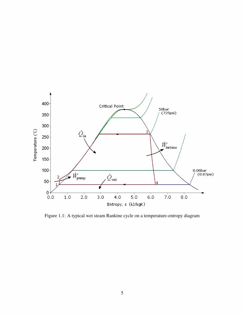
Figure 1.1: A typical wet steam Rankine cycle on a temperature-entropy diagram
5
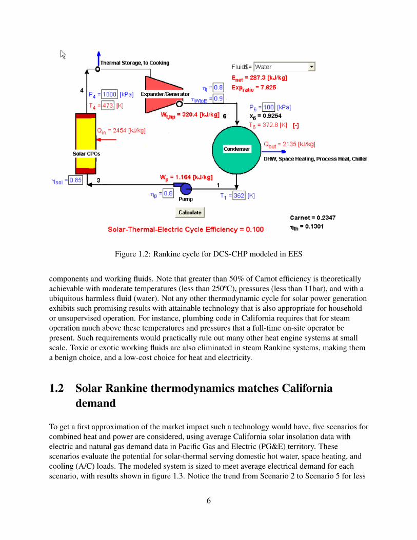
Figure 1.2: Rankine cycle for DCS-CHP modeled in EES
components and working fluids. Note that greater than 50% of Carnot efficiency is theoreticallyachievable with moderate temperatures (less than 250ºC), pressures (less than 11bar), and with aubiquitous harmless fluid (water). Not any other thermodynamic cycle for solar power generationexhibits such promising results with attainable technology that is also appropriate for householdor unsupervised operation. For instance, plumbing code in California requires that for steamoperation much above these temperatures and pressures that a full-time on-site operator bepresent. Such requirements would practically rule out many other heat engine systems at smallscale. Toxic or exotic working fluids are also eliminated in steam Rankine systems, making thema benign choice, and a low-cost choice for heat and electricity.
1.2 Solar Rankine thermodynamics matches Californiademand
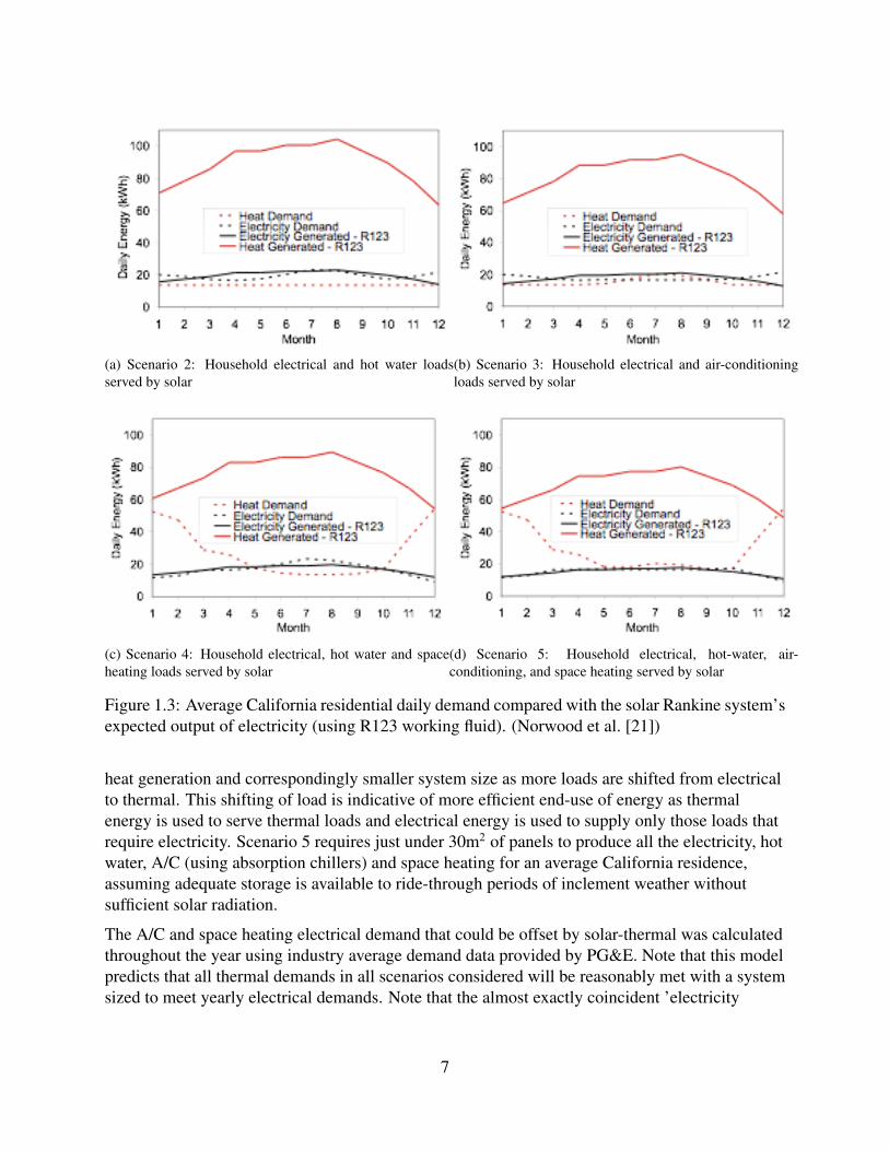
To get a first approximation of the market impact such a technology would have, five scenarios forcombined heat and power are considered, using average California solar insolation data withelectric and natural gas demand data in Pacific Gas and Electric (PG&E) territory. Thesescenarios evaluate the potential for solar-thermal serving domestic hot water, space heating, andcooling (A/C) loads. The modeled system is sized to meet average electrical demand for eachscenario, with results shown in figure 1.3. Notice the trend from Scenario 2 to Scenario 5 for less
6
(a) Scenario 2: Household electrical and hot water loadsserved by solar
(b) Scenario 3: Household electrical and air-conditioningloads served by solar
(c) Scenario 4: Household electrical, hot water and spaceheating loads served by solar
(d) Scenario 5: Household electrical, hot-water, air-conditioning, and space heating served by solar
Figure 1.3: Average California residential daily demand compared with the solar Rankine system’sexpected output of electricity (using R123 working fluid). (Norwood et al. [21])
heat generation and correspondingly smaller system size as more loads are shifted from electricalto thermal. This shifting of load is indicative of more efficient end-use of energy as thermalenergy is used to serve thermal loads and electrical energy is used to supply only those loads thatrequire electricity. Scenario 5 requires just under 30m2 of panels to produce all the electricity, hotwater, A/C (using absorption chillers) and space heating for an average California residence,assuming adequate storage is available to ride-through periods of inclement weather withoutsufficient solar radiation.
The A/C and space heating electrical demand that could be offset by solar-thermal was calculatedthroughout the year using industry average demand data provided by PG&E. Note that this modelpredicts that all thermal demands in all scenarios considered will be reasonably met with a systemsized to meet yearly electrical demands. Note that the almost exactly coincident ’electricity
7
demand’ and ’electricity generated’ curves indicate a good temporal match of average demand toaverage production of the DCS-CHP system for this central California location. Note also that theresult in scenarios 2 and 5 assumes heat driven absorption or adsorption cooling systems are inwidespread use, although small customers rarely use these systems today. This analysis is notindicative of actual energy demand or output for any given California residence or solar system,but is nonetheless useful in determining how, in aggregate, wide-scale dissemination ofDCS-CHP systems could meet our current California energy demands. The applicability of thistechnology in other locations will of course depend on the shape of their respective load curves.
1.3 Performance-Cost analysis of solar combined heat andpower systems
Solar combined heat and power (CHP) systems can compete or exceed solar photovoltaics (PV) –which is often used as the benchmark in terms of efficiency, performance, and cost – in a range ofdistributed generation applications, and across a range of specific technology platforms. Acommon metric to evaluate the cost of photovoltaics is a cost per peak power output or “dollarsper watt” metric. For the purpose of comparison, we develop a new analytic methodology toevaluate the cost of the electricity generated from a solar CHP system. The electricity generationand thermal subsystems of a solar CHP system are energetically intertwined, yet by comparingthermal and electrical outputs a sensible cost division can be determined. This method is thenused to compare the cost of stationary PV and solar Rankine CHP systems with tracking andstationary collectors. The capacity factors of electricity generation for each system is found insimulation using NREL TMY3 climatic data for 1020 sites in the United States. The solarRankine system with stationary collectors outperforms the PV system in warmer and sunnierclimates relative to its rated “dollar per watt” output, while PV outperforms solar Rankine incooler climates. With tracking concentrating collectors, the solar Rankine system outperforms PVsystems in the vast majority of US sites at an estimated cost of $4/W and a collector hightemperature of 250°C. In conclusion, a PV system and solar Rankine CHP system, sized equallyin terms of peak power output, will produce comparable amounts of electricity (+/- 10% onaverage), however the solar Rankine CHP system will additionally provide 4 to 6 units of usefulheat energy for every one unit of electricity generated.
1.3.1 Nomenclature
c Overall cost of peak electrical output!
$Wel
"
ce Electric power subsystem cost per unit of peak output!
$Wel
"
C Overall cost per unit area of collector# $
m2
$
Cc Collector subsystem cost per unit area of collector# $
m2
$
8
Cx Collector subsystem cost not offset by heat production, per unit area of collector# $
m2
$
Ce Electric power subsystem cost per unit area of collector# $
m2
$
!c Collector efficiency
!0 Carnot efficiency of Rankine cycle
!p Fraction of Carnot efficiency achieved in Rankine cycle
!r Overall efficiency of Rankine cycle
!t Fraction of waste heat recovered from Rankine cycle
G Reference insolation level# W
m2
$
Pc Collector heat output per unit area of collector#Wth
m2
$
Pt Useful heat output of system#Wth
m2
$
Px Heat output of heat-only system not offset by CHP heat output
Pe Electrical power output of system#Wel
m2
$
Q Solar CHP to PV yearly performance ratio
R Actual ratio of thermal to electrical power output
Rd Desired ratio of thermal to electrical power output
Ta Ambient temperature [K]
Th Rankine cycle high temperature (expander inlet) [K]
Tm Heating load supply temperature (collector or expander outlet) [K]
Tl Heating load return temperature (collector inlet) [K]
WCHP CHP system’s electrical energy produced over a year [J]
WPV PV system’s electrical energy produced over a year [J]
E,A,B Collector performance coefficients [%],# W
m2K
$,# W
m2K2
$
[ ]! Starred quantities refer to system producing heat only
[ ] Barred quantities refer to systems at reference conditions
9
1.3.2 Performance-Cost methodology
Distributed solar electric systems currently use photovoltaics almost exclusively. These systemsare often compared on the basis of “dollars per watt,” which represents the total cost of theinstallation divided by its peak electrical power output. Since different photovoltaic (PV) systemscan be expected to react similarly under changing conditions, it is reasonable to compare them onthe basis of this single reference point.
Solar combined heat and power (CHP) systems, however, produce both electricity and usefulheat. While this dual output makes solar CHP systems potentially more valuable in distributedapplications, it also makes their value more difficult to quantify and compare. Onestraightforward solution is to compare the overall costs and long term outputs of potential systemsfor a specific application. This method, however, produces application specific results that are noteasily generalized.
Instead, an analytical method is developed to enable direct comparison of solar combined heatand power and PV technologies, based on the existing metric of dollars per peak electrical watt. Itis intended to capture the major factors that affect solar CHP system performance, such ascollector performance, unit costs, temperature limits, and efficiencies. At the same time, itattempts to avoid application specific information like system size and local meteorology.
Here, the method is developed for two variations on a solar Rankine system with either stationaryevacuated tube collectors, or tracking concentrating dish collectors supplying heat to a Rankinecycle. The method is described conceptually, then derived analytically. The method is then usedto estimate the cost of solar Rankine CHP systems with different types of collectors, and tocompare them to PV systems. The assumption that PV and solar Rankine systems can becompared on the basis of this one reference point (cost per peak electrical watt) is tested bycomparing the model to a parametrization of the real-world relative performance of each system.While the behavior of PV and solar CHP systems can diverge considerably under somecircumstances, the systems are found to behave with reasonable similarity overall in terms ofaverage electrical output. Thus, the “dollars per watt” metric represents overall performance wellenough to justify its use in the preliminary design of solar Rankine systems, and in generalizedcomparisons to photovoltaics. In terms of heat output, the solar Rankine system will provide 4 to6 units of thermal energy and one unit of electrical energy for every one unit of electrical energyproduced by the same size (peak Watts electric) PV system.
To evaluate distributed solar CHP systems on the basis of cost per peak electrical watt, it isnecessary to account for the value of the useful heat that is also produced. This is done byconceptually dividing the system into two parts: a collector subsystem and a power generationsubsystem. The collector subsystem consists of the solar collectors and their associatedequipment, such that it could embody a stand-alone solar heating system. It is assumed that thishypothetical stand-alone system would produce heat cost effectively (a reasonable assumption,since the collector technology is designed for solar hot water applications). The power generationsubsystem consists of all the additional equipment necessary to produce electrical power from thethermal output of the collector subsystem.
With the system divided as such, it is now possible to determine the cost of its electrical output.
10
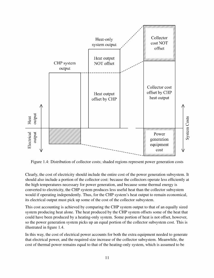
Figure 1.4: Distribution of collector costs; shaded regions represent power generation costs
Clearly, the cost of electricity should include the entire cost of the power generation subsystem. Itshould also include a portion of the collector cost: because the collectors operate less efficiently atthe high temperatures necessary for power generation, and because some thermal energy isconverted to electricity, the CHP system produces less useful heat than the collector subsystemwould if operating independently. Thus, for the CHP system’s heat output to remain economical,its electrical output must pick up some of the cost of the collector subsystem.
This cost accounting is achieved by comparing the CHP system output to that of an equally sizedsystem producing heat alone. The heat produced by the CHP system offsets some of the heat thatcould have been produced by a heating-only system. Some portion of heat is not offset, however,so the power generation system picks up an equal portion of the collector subsystem cost. This isillustrated in figure 1.4.
In this way, the cost of electrical power accounts for both the extra equipment needed to generatethat electrical power, and the required size increase of the collector subsystem. Meanwhile, thecost of thermal power remains equal to that of the heating-only system, which is assumed to be
11
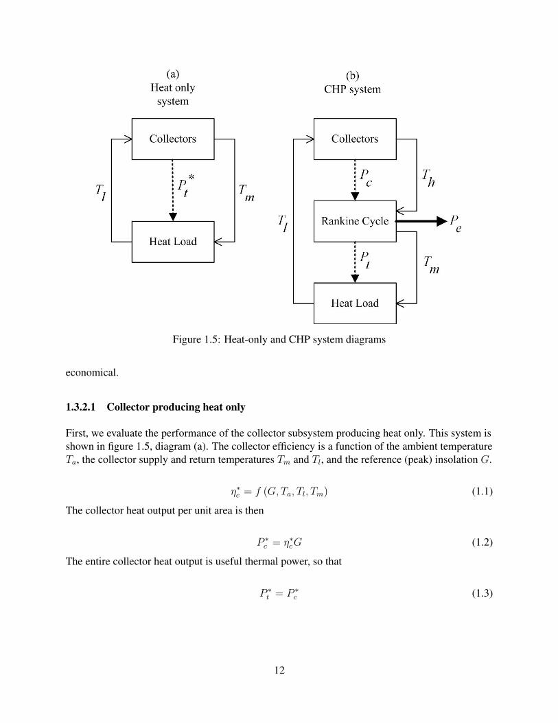
Figure 1.5: Heat-only and CHP system diagrams
economical.
1.3.2.1 Collector producing heat only
First, we evaluate the performance of the collector subsystem producing heat only. This system isshown in figure 1.5, diagram (a). The collector efficiency is a function of the ambient temperatureTa, the collector supply and return temperatures Tm and Tl, and the reference (peak) insolation G.
!!c = f (G, Ta, Tl, Tm) (1.1)
The collector heat output per unit area is then
P !c = !!cG (1.2)
The entire collector heat output is useful thermal power, so that
P !t = P !
c (1.3)
12
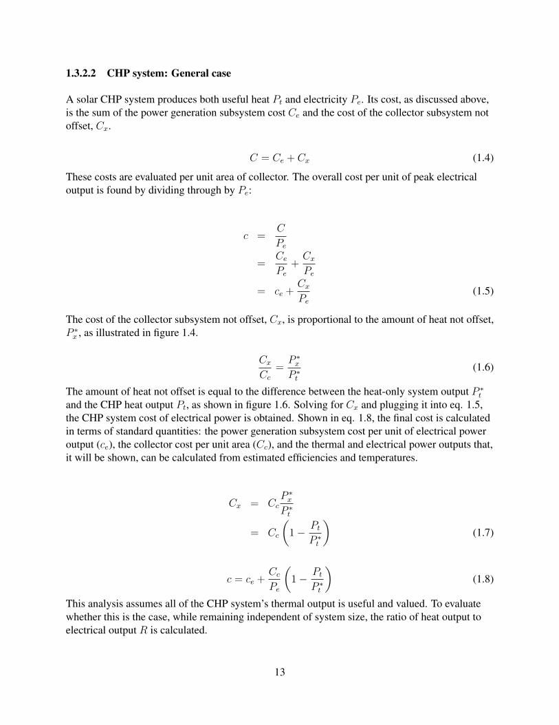
1.3.2.2 CHP system: General case
A solar CHP system produces both useful heat Pt and electricity Pe. Its cost, as discussed above,is the sum of the power generation subsystem cost Ce and the cost of the collector subsystem notoffset, Cx.
C = Ce + Cx (1.4)
These costs are evaluated per unit area of collector. The overall cost per unit of peak electricaloutput is found by dividing through by Pe:
c =C
Pe
=Ce
Pe+
Cx
Pe
= ce +Cx
Pe(1.5)
The cost of the collector subsystem not offset, Cx, is proportional to the amount of heat not offset,P !x , as illustrated in figure 1.4.
Cx
Cc=
P !x
P !t
(1.6)
The amount of heat not offset is equal to the difference between the heat-only system output P !t
and the CHP heat output Pt, as shown in figure 1.6. Solving for Cx and plugging it into eq. 1.5,the CHP system cost of electrical power is obtained. Shown in eq. 1.8, the final cost is calculatedin terms of standard quantities: the power generation subsystem cost per unit of electrical poweroutput (ce), the collector cost per unit area (Cc), and the thermal and electrical power outputs that,it will be shown, can be calculated from estimated efficiencies and temperatures.
Cx = CcP !x
P !t
= Cc
%1! Pt
P !t
&(1.7)
c = ce +Cc
Pe
%1! Pt
P !t
&(1.8)
This analysis assumes all of the CHP system’s thermal output is useful and valued. To evaluatewhether this is the case, while remaining independent of system size, the ratio of heat output toelectrical output R is calculated.
13
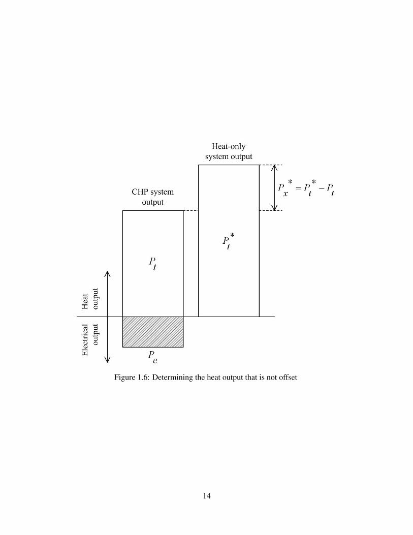
Figure 1.6: Determining the heat output that is not offset
14
R =Pt
Pe(1.9)
If this ratio is too large for the application, a desired ratio Rd can be substituted for R. Forexample, California homes consume about one to five times as much thermal energy as electrical,depending on the season (Norwood et al. [21]).
Rd =Pt"useful
Pe(1.10)
" R
Of course, if less heat is useful and valued, then less of the collector subsystem cost is offset, andthe cost of the CHP system’s electrical output will rise accordingly. Eq. 1.11 gives the cost ofelectrical power in terms of the desired heat-to-electricity ratio Rd.
c = ce +Cc
Pe
%1! Pt"useful
P !t
&
= ce +Cc
Pe! CcRd
P !t
(1.11)
1.3.2.3 Rankine cycle power: Special case
In the previous section, the analysis considered a solar CHP system supplying arbitrary heat andpower outputs. Now, a special case is considered, wherein the collector output is used to run aRankine cycle at a high temperature Th. The heat load is supplied by waste heat rejected from theRankine cycle condenser at temperature Tm, and working fluid returns to the collector at lowtemperature Tl. This system is shown schematically in diagram (b) of figure 1.5. The collectorefficiency is recalculated in terms of Th:
!c = f (G, Ta, Tl, Th) (1.12)
The overall Rankine cycle efficiency !r is a function of the Carnot efficiency !0 (which is themaximum theoretical efficiency for any heat engine operating between a high temperature sourceand low temperature sink) and the anticipated percent of the Carnot efficiency the cycle isexpected to achieve, !p.
!r = !p!0
= !p
%1! Tm
Th
&(1.13)
15
The CHP system’s heat and electricity outputs (as always, per unit area of collector) are functionsof these efficiencies and the fraction of waste heat that is expected to be recovered for use by theheating load (!t). As such, Pe and Pt are no longer arbitrary. Rather, they are determined by thespecific solar CHP scheme under consideration: its structure, temperatures, and expectedefficiencies.
Pe = !rPc
= !r!cG (1.14)
Pt = (1! !r) !tPc
= (1! !r) !t!cG (1.15)
The cost of electricity is calculated by plugging Pe and Pt into eq. 1.8. As before, this costrepresents the total cost per peak watt of electrical output. It is independent of system size (to theextent that its inputs are independent of system size) and is a function of unit component costs,temperatures, and anticipated efficiencies.
c = ce +Cc
Pe
%1! Pt
P !t
&
= ce +Cc
!r!cG
%1! (1! !r) !t!cG
!!cG
&
= ce +Cc
G
%1
!r!c! !t
!r!!c+
!t!!c
&(1.16)
The ratio of thermal to electrical power output R of this system is
R =(1! !r) !t!cG
!r!cG
= !t
%1
!r! 1
&(1.17)
If less heat is required per unit electrical output, eq. 1.16 is recalculated using Rd:
c = ce +Cc
Pe! CcRd
P !t
= ce +Cc
G
%1
!r!c! Rd
!!c
&where Rd " !t
%1
!r! 1
&(1.18)
16
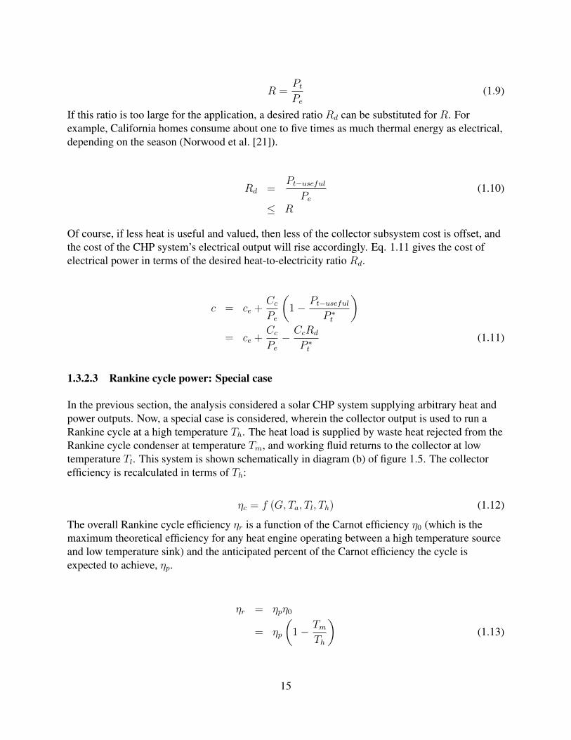
1.3.3 Application to a potential system
The cost of a solar Rankine CHP system, like the one described in the previous section, isestimated using the properties listed in Table 1.1with sources. In this table, estimates are providedfor a steam Rankine cycle heat engine achieving 50% of Carnot efficiency in electrical generationoperating at the high and low temperatures indicated with 80% waste heat recovery. Threehypothetical systems are compared using different collector arrays, all assumed to have the samecost per aperture area. Two systems use evacuated tube collectors with efficiency calculated usingeq. 1.19, given manufacturer supplied constants E, A, and B.
!!c = E ! A
G
%Tinlet + Toutlet
2! Ta
&! B
G
%Tinlet + Toutlet
2! Ta
&2
(1.19)
The third system uses a model for a tracking concentrating dish collector, where the collectorperformance coefficients come from published data for a trough collector (trough coefficients arecomparable to those for a dish collector). Direct normal solar insolation is used in eq. 1.19 tocalculate collector efficiency. Rather than being fixed from the outset, the collector outputtemperature Th is varied to find the operating point that minimizes the installed cost of electricity.All other things being equal, because collector efficiency decreases and Rankine cycle efficiencyincreases with increasing collector temperature, there is a minimum (optimum) cost point forthese systems. Using these values and eq. 1.16 the installed cost of this hypothetical system withnon-concentrating evacuated tube collectors would be about $6.00/Wel, at an optimal collectoroutput temperature of approximately170#C, and with tracking dish collectors would be $4/Wel ata collector temperature of 250#C, as seen in figure 1.7. This cost compares favorably toresidential (Pe < 10kW) photovoltaic systems that were $7.90/Wel installed in 2007(Wiser et al.[44]). The relative thermal to electric output ratio for the evacuated tube systems would beapproximately 6:1, and for the dish system 4:1.
This cost assumes that all of the heat produced (in this case 4-6 units of heat for every unit ofelectricity) is useful. If the demand for heat is less (Rd < R), the cost of electricity rises as doesthe optimal collector output temperature. This suggests that solar Rankine systems will be mosteconomical where there exists a large demand for low temperature heat (below 100#C) relative todemand for electricity. In such cases, Rd = R: the entire waste heat stream is useful and valued,so the cost of electricity is minimized.
1.4 Verification of the model for comparison to PV
The cost metric developed here considers system performance at a specific set of referenceconditions (essentially summer peak performance). While it may suggest that a specific solarRankine system is cost competitive with PV, this conclusion is supported only at such conditions.At other conditions, which depend on location, weather, and diurnal and seasonal variations, theperformance of a solar CHP system to that of a PV system remains unknown. For example, onecould imagine a solar CHP system that performed brilliantly in ideal conditions, but dismally in
17
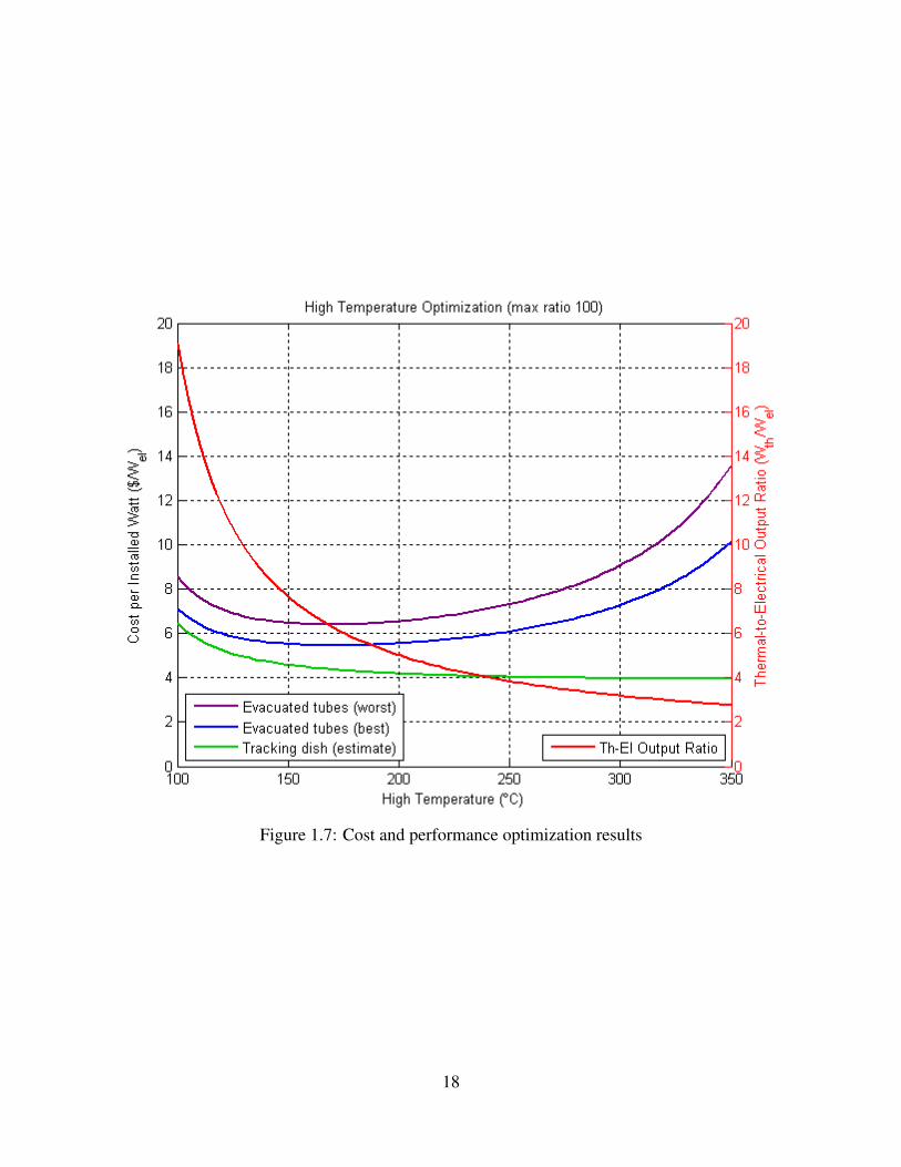
Figure 1.7: Cost and performance optimization results
18
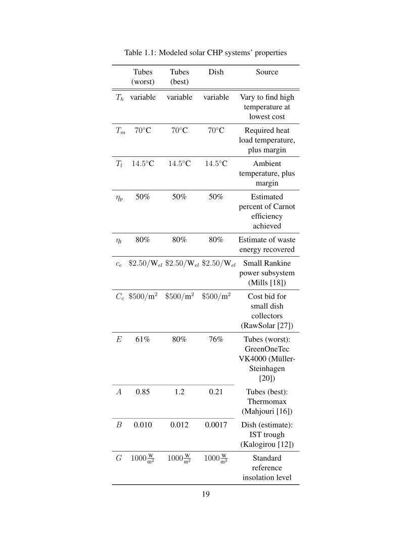
Table 1.1: Modeled solar CHP systems’ properties
Tubes(worst)
Tubes(best)
Dish Source
Th variable variable variable Vary to find hightemperature at
lowest cost
Tm 70#C 70#C 70#C Required heatload temperature,
plus margin
Tl 14.5#C 14.5#C 14.5#C Ambienttemperature, plus
margin
!p 50% 50% 50% Estimatedpercent of Carnot
efficiencyachieved
!t 80% 80% 80% Estimate of wasteenergy recovered
ce $2.50/Wel $2.50/Wel $2.50/Wel Small Rankinepower subsystem
(Mills [18])
Cc $500/m2 $500/m2 $500/m2 Cost bid forsmall dishcollectors
(RawSolar [27])
E 61% 80% 76% Tubes (worst):GreenOneTec
VK4000 (Müller-Steinhagen
[20])
A 0.85 1.2 0.21 Tubes (best):Thermomax
(Mahjouri [16])
B 0.010 0.012 0.0017 Dish (estimate):IST trough
(Kalogirou [12])
G 1000 Wm2 1000 W
m2 1000 Wm2 Standard
referenceinsolation level
19
marginal conditions. This system would appear competitive in terms of cost per peak electricalwatt, but would perform poorly on the whole.
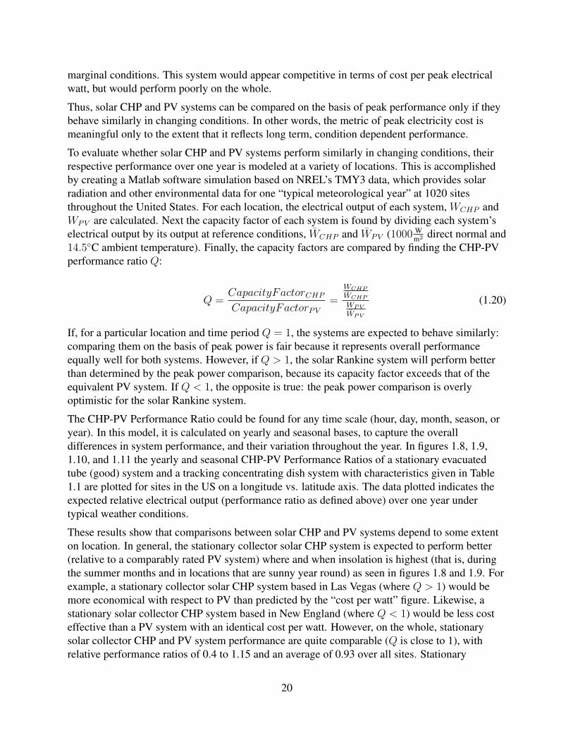
Thus, solar CHP and PV systems can be compared on the basis of peak performance only if theybehave similarly in changing conditions. In other words, the metric of peak electricity cost ismeaningful only to the extent that it reflects long term, condition dependent performance.
To evaluate whether solar CHP and PV systems perform similarly in changing conditions, theirrespective performance over one year is modeled at a variety of locations. This is accomplishedby creating a Matlab software simulation based on NREL’s TMY3 data, which provides solarradiation and other environmental data for one “typical meteorological year” at 1020 sitesthroughout the United States. For each location, the electrical output of each system, WCHP andWPV are calculated. Next the capacity factor of each system is found by dividing each system’selectrical output by its output at reference conditions, WCHP and WPV (1000 W
m2 direct normal and14.5#C ambient temperature). Finally, the capacity factors are compared by finding the CHP-PVperformance ratio Q:
Q =CapacityFactorCHP
CapacityFactorPV=
WCHP
WCHP
WPV
WPV
(1.20)
If, for a particular location and time period Q = 1, the systems are expected to behave similarly:comparing them on the basis of peak power is fair because it represents overall performanceequally well for both systems. However, if Q > 1, the solar Rankine system will perform betterthan determined by the peak power comparison, because its capacity factor exceeds that of theequivalent PV system. If Q < 1, the opposite is true: the peak power comparison is overlyoptimistic for the solar Rankine system.
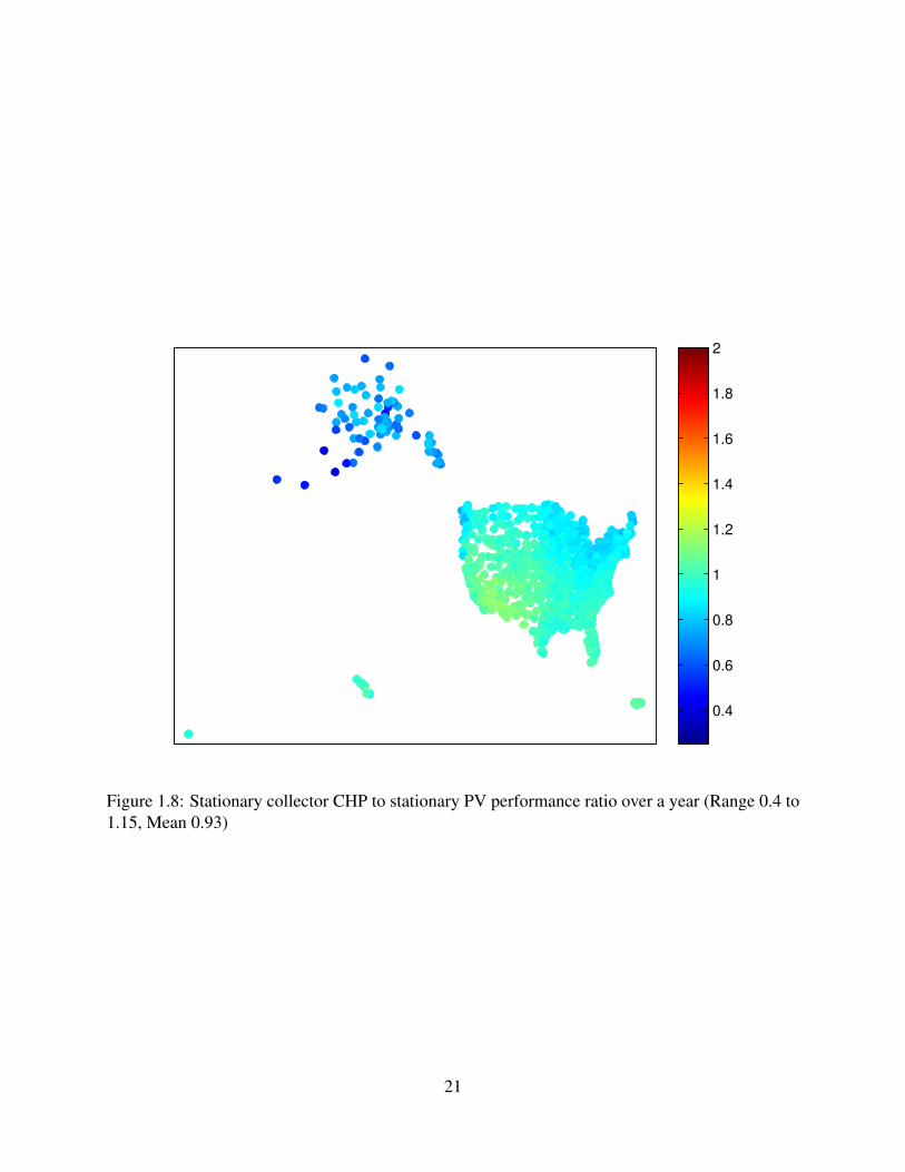
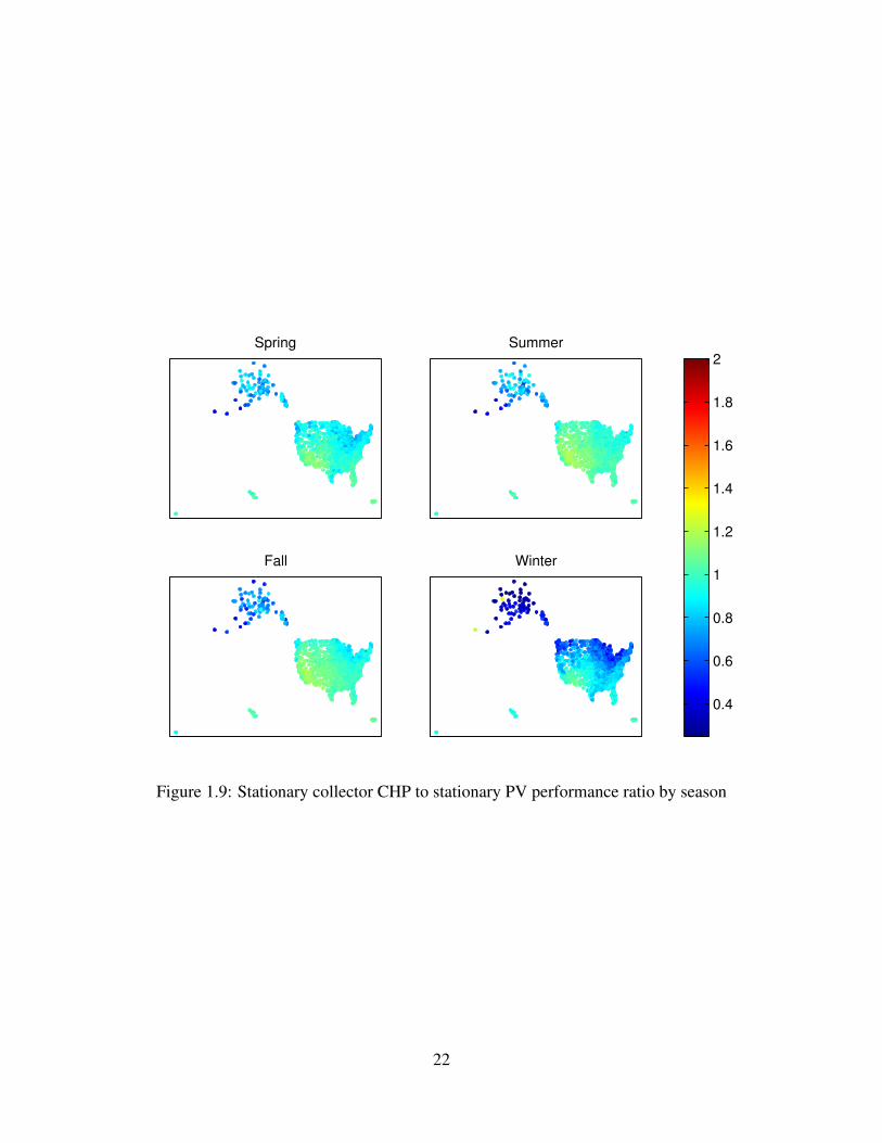
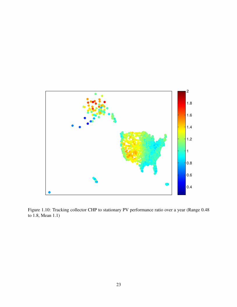
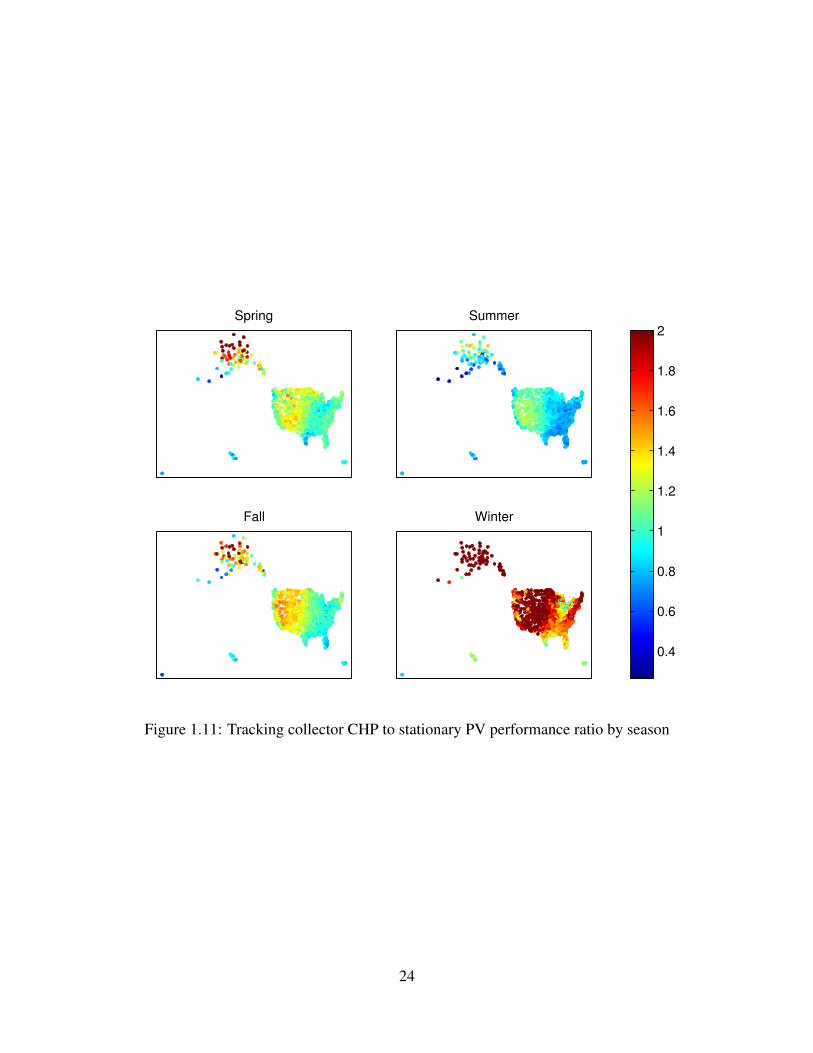
The CHP-PV Performance Ratio could be found for any time scale (hour, day, month, season, oryear). In this model, it is calculated on yearly and seasonal bases, to capture the overalldifferences in system performance, and their variation throughout the year. In figures 1.8, 1.9,1.10, and 1.11 the yearly and seasonal CHP-PV Performance Ratios of a stationary evacuatedtube (good) system and a tracking concentrating dish system with characteristics given in Table1.1 are plotted for sites in the US on a longitude vs. latitude axis. The data plotted indicates theexpected relative electrical output (performance ratio as defined above) over one year undertypical weather conditions.
These results show that comparisons between solar CHP and PV systems depend to some extenton location. In general, the stationary collector solar CHP system is expected to perform better(relative to a comparably rated PV system) where and when insolation is highest (that is, duringthe summer months and in locations that are sunny year round) as seen in figures 1.8 and 1.9. Forexample, a stationary collector solar CHP system based in Las Vegas (where Q > 1) would bemore economical with respect to PV than predicted by the “cost per watt” figure. Likewise, astationary solar collector CHP system based in New England (where Q < 1) would be less costeffective than a PV system with an identical cost per watt. However, on the whole, stationarysolar collector CHP and PV system performance are quite comparable (Q is close to 1), withrelative performance ratios of 0.4 to 1.15 and an average of 0.93 over all sites. Stationary
20
0.4
0.6
0.8
1
1.2
1.4
1.6
1.8
2
Figure 1.8: Stationary collector CHP to stationary PV performance ratio over a year (Range 0.4 to1.15, Mean 0.93)
21
Spring Summer
Fall Winter
0.4
0.6
0.8
1
1.2
1.4
1.6
1.8
2
Figure 1.9: Stationary collector CHP to stationary PV performance ratio by season
22
0.4
0.6
0.8
1
1.2
1.4
1.6
1.8
2
Figure 1.10: Tracking collector CHP to stationary PV performance ratio over a year (Range 0.48to 1.8, Mean 1.1)
23
Spring Summer
Fall Winter
0.4
0.6
0.8
1
1.2
1.4
1.6
1.8
2
Figure 1.11: Tracking collector CHP to stationary PV performance ratio by season
24
collector solar CHP system performance is especially advantaged where insolation is highest.Thus, the cost per watt metric is most conservative with respect to solar CHP systems in locationswhere it makes the most sense to utilize a solar power system to begin with.
Comparing tracking solar CHP systems to stationary PV yields a very different seasonal resultseen in figure 1.11, but the same general comparability exists in overall capacity factors for thetwo systems. The tracking system (always facing the sun) when compared to a stationary PVsystem (tilted at latitude) will perform much better in many northerly locations, like Alaska,because cosine losses will be highest for the stationary collectors in that season. The tracking dishsystem will also outperform the PV system in locations where most sunlight is direct, and littlediffuse light is collected. Because aperture angle and concentration are inversely related, thetracking collector is unable to collect much light on cloudy days, whereas the stationary system isrelatively good at collecting diffuse light coming from a wide swath of sky. The modeled range ofperformance ratios of tracking collector solar CHP to stationary PV is 0.48 to 1.8, and 1.1 onaverage over all sites.
1.5 Discussion and conclusions
A sensitivity analysis of the modeling results discussed in this chapter shows that collector costs,collector efficiency, and expander efficiency most heavily influence the cost results. This isintuitive based on the efficiency calculations derived earlier in this chapter. For instance, it is notsurprising that the pump’s isentropic efficiency has a relatively small effect on solar-electricsystem efficiency, given that pump work is on the order of 1% of the turbine output in thisRankine cycle. Collector efficiency and expander efficiency, on the other hand, heavily influencethe cost of the system because the collector array is such an expensive component, and anysignificant decrease in either the collector efficiency or that of the heat engine significantlyimpacts the levelized cost of energy generated. The efficiency and pressure ratio of the expanderare the most important variables in determining overall heat engine efficiency and also have alarge effect on the ratio of electric to thermal energy delivered. Both the generator and thecollector are multiplicative factors in determining overall solar-electric efficiency, so largeimpacts in levelized cost are also observed when varying these parameters.
The analysis in this chapter ignores the fact that there are real costs associated with theinfrastructure necessary to use the heat collected by a solar CHP system. In reality, technologicalsynergies do exist between human needs and different sources of heat. For instance, houses in theUnited States are typically heated by forced air furnaces or radiant systems (such as radiant floors,baseboard radiators, etc.). For retrofits, radiant heating is probably more suited to integration witha DCS-CHP system than is forced-air heating because the radiant heating system operates attemperatures low enough to use the waste heat from a Rankine cycle. Also, the higher latency anduse of thermal mass in radiant-type systems lends itself well to an intermittent energy supply likethe sun. Forced-air systems, on the other hand, tend to have lower latency, and would also requirea liquid-air heat exchanger as opposed to the more cost effective liquid-liquid heat exchanger usedin radiant systems. Cooking is another area where the type of use dictates the usefulness of waste
25
heat. Typical stove top cooking temperatures far exceed the condensation temperature of aDCS-CHP Rankine cycle, yet some communities have successfully set up solar pressure cookersat temperatures appropriate for DCS-CHP (Weisman [41]), showing that it is possible toreconstruct the built environment to be more suited to solar thermal energy sources. Airconditioning is a different story: Typical heat-driven absorption and adsorption systems operate attemperatures low enough to use the heat from a DCS-CHP system, however price has limitedsmall-scale application of thermally-driven cooling. As electric compressor chillers become moreefficient there is also competitive pressure for heat-driven cooling systems to become morecost-effective (Norwood et al. [22]). As can be seen from these varied thermal end uses, there aresome places where a DCS-CHP system would reduce the cost of auxillary infrastructure, andother places where it would increase the cost (e.g. in retrofits). This is to say nothing of thepotential need for thermal storage or a non-solar back-up when operating with a DCS-CHPsystem, neither of which are explored here. Instead this analysis focuses on the cost of deliveringa unit of solar thermal and solar electric energy from a DCS-CHP system; a discussion that iscontinued in Chapter 2 along with the introduction of DCS-CHP and water desalination.
In this chapter we looked at California demand and a simple model to compare average demandwith expected output of a DCS-CHP system, concluding that thermal and electrical loads are wellmatched to system production. We then develop a methodology for sensibly disentangling thecosts of electrical and heat production from a solar combined heat and power system. Usingtypical meteorological year solar data we compare the output of a solar Rankine CHP system withan identically sized (in terms of peak power) photovoltaic system. This shows that within a boundof plus or minus 10%, with either tracking or stationary collectors, that the average electrical costof a solar CHP system is comparable to that of a stationary PV system in terms of “cost per watt”.However, the solar Rankine CHP system will additionally provide 4 to 6 units of useful heatenergy for every one unit of electricity generated whereas the typical photovoltaic system willprovide no useful heat. For the purposes of research and development into solar Rankine CHPsystems, peak power rating is therefore a metric that permits fair comparison of solar CHPelectrical output to distributed photovoltaics of power less than 10kW. However, due to theextreme variations in weather patterns and the differential effects of these patterns on systemoutput, site specific weather data is necessary to realistically predict and compare the levelizedcost of electricity production for these two systems.
26

Chapter 2
Life Cycle Analysis: Economics, GlobalWarming Potential, and Water forDistributed Concentrating Solar CombinedHeat and Power
27
2.1 Introduction
Ultimately, the goal of this project is to develop an energy generation system that utilizes arenewable energy source (the sun) while working towards mitigation of global climatedestabilization. To ensure this goal is achieved the following three steps are necessary: (1)determine and utilize appropriate metrics for solar energy technology (2) establish and utilizemethods for life-cycle assessment (LCA) of emerging technologies (3) optimize the system basedon the chosen metrics and LCA results.
Many assessments of alternative energy systems have focused on the energy payback time of thesystem, however given the goal of mitigating climate chaos at the lowest possible cost, moreappropriate metrics to use are greenhouse gas intensity and life cycle costing. Greenhouse gasintensity, indicating the units of GHG emissions produced for every unit of electricity or heatgenerated over the system lifetime, improves upon energy metrics that fail to appropriatelyacknowledge the different global warming potentials of working fluids or differences in fuelsources used during manufacturing of components. For specific sites, other LCA metrics likeGreenhouse Gas Return on Investment, and the Water Availability Factor would be appropriatefor assessing appropriateness of distributed concentrating solar combined heat and power(Reich-Weiser et al. [28]). The economic input-output life-cycle assessment (EIOLCA) databaseprovided by Carnegie Mellon University can provide economic life cycle data with appropriatecategorization of system component costs into EIOLCA categories (Hendrickson et al. [9]).These metrics and other environmental considerations are incorporated early in this designprocess, given only cost and materials estimates. As development of a particular design movesforward, more detailed process-based analysis (Pehnt [24]) can be used to understand design tradeoffs between environmental, performance, and economic goals. In addition to greenhouse gasemissions, water use and toxicity are assessed as decisions are made on materials and functionalform.
To these ends, the first part of this chapter is devoted to LCA economics and GWP analysis of aproposed DCS-CHP system, and the latter part of this chapter explores the water use and potentialfor water purification/desalination using DCS-CHP. For the purposes of life cycle analysis, theproblem of joint production makes it difficult to allocate the relative costs of a CHP system toelectrical and heat production (Wade [40]) so costs are divided using the methodology describedin Chapter 1 (Norwood et al. [23]).
2.2 Life Cycle Assessment of a single solar dish collectorDCS-CHP system
Performing a life cycle assessment (LCA) is a useful way of comparing the environmentalimpacts of different power generation systems. Here, a life cycle assessment is completed on asingle solar dish collector solar Rankine combined heat and power system using the IndustryBenchmark US Department of Commerce EIO model from 1997 (Hendrickson et al. [9]). Theglobal warming potential (GWP) per kWh of energy, the energy payback time (EPBT), the cost
28
per installed peak watt, and the levelized cost of electrical and thermal energy are calculated.These results show DCS-CHP generates an estimated GWP of 80 gCO2 equivalent greenhousegases per kWh electricity, putting it below the competitive range with photovoltaics (PV), whichrange from 110-180 gCO2eq/kWh according to a couple recent studies(Stoppato [34], Lenzen[14]). The EPBT for the DCS-CHP system, estimated at 27 months, makes it competitive with PVsystems. The levelized cost of energy generated by the DCS-CHP system over its lifetime isestimated to be $0.25/kWh electric, and $0.03/kWh of 100ºC heat, or $3.20/W electric and$0.40/W thermal in terms of installed capital cost per peak power output. The LCA of the systemaffirms that small scale solar combined heat and power systems can economically compete withother renewable energy systems and have comparable environmental footprints to PV systems.
2.2.1 Assumptions of LCA
The Industry Benchmark US Department of Commerce EIO model from 1997 adjusted forinflation, with the breakdown of selected sectors shown in Figure 2.1, provides a basis for thisLCA.
The RawSolar prototype collector (RawSolar [27]), with the performance parameters specified inChapter 1 for a dish collector, provides an estimate of collector efficiency. Using the data for theKatrix rotary lobe expander from Chapter 3, and NREL typical meteorological year solarinsolation data for Oakland, CA along with the collector efficiency, we run the DCS-CHPmodeling software parameterized as described in Chapter 4. Working from a cost estimate fromRawSolar complete with bids for materials and labor (for installing the concentrating solarthermal system in Richmond, CA) we add the necessary components for electricity generation tocome up with a final system cost as broken down in Table 2.1. Costs are divided betweenelectrical and heat generation according to the methodology described in Chapter 1. Thesimplified levelized energy cost LEC assuming fixed yearly operation and maintenance costs Mover the lifetime of 25 years n, a 7% interest rate r, the initial capital costs I , and total energyproduced per year E is (Appropedia [2]):
LEC =I'
r1"(1+r)!n
(+M
E(2.1)
2.2.2 LCA of economics and GWP results
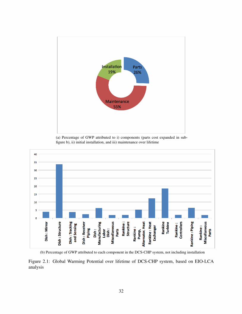
The DCS-CHP system is estimated to produce ~80 gCO2eq/kWh of electricity and ~10gCO2eq/kWh thermal assuming the 1997 mix of fuels reported in the US EIO database. This ismuch less than fossil fuel based power generation methods, which produce hundreds ofgCO2eq/kWh. In comparison to renewable energy technologies, according to Lenzen, theDCS-CHP system GWP is higher than that of wind turbines (21 gCO2eq/kWh) andhydroelectricity (15 gCO2eq/kWh) but lower than photovoltaics (106 gCO2eq/kWh) (Lenzen[14]). Overall, the GWP contribution of the DCS-CHP system was split evenly between the dish
29
(a) Cost estimates, sector references, and associated GWP (gCO2 equivalent) based on EIO-LCA for the RawSolarconcentrating dish components
(b) Cost estimates, sector references, and associated GWP (gCO2 equivalent) based on EIO-LCA for the other systemcomponents
Table 2.1: Cost estimates and EIO-LCA data for DCS-CHP system
30
components and the Rankine cycle components. Most of the GWP contribution comes frommaintenance of the dish and Rankine cycle components as seen in Figure 2.1a. Considering theGWP of only the initial components, Figure 2.1b shows that the dish structure and the Rankineexpander contribute the majority of the GWP.
This analysis predicts a single dish collector system with peak capacity of ~1kW electric wouldproduce electricity for $3.20/W capital cost and a levelized cost of electricity of $0.25/kWh.Local electricity rates in the San Francisco Bay Area are about $0.14/kWh, but in the author’sexperience, many larger households pay more for electricity because of increasing block tariffs.The DCS-CHP system is additionally expected to produce useful heat energy with a peakcapacity of ~5kW (80% waste-heat recovery factor) for a capital cost of $0.40/W or levelized costof $0.03/kWh. Energy Payback Time (EPBT) for our system, including both electricity and heatproduction, is expected to be 27 months.
2.3 Water and solar energy
The ties between water and solar energy are inextricable. The sun drives the giant distillationprocess called the hydrological cycle. The energy from sunlight evaporates water, 97% of whichis saline, covering three-quarters of the earth’s surface, and transforms it into fresh water vapor,condenses it in the atmosphere in the form of clouds, transports it via wind, and delivers much ofit to the land as rain where it fills our rivers, lakes and aquifers. Humans often replicate this cycle,which has been occurring endlessly for eons, albeit on a more modest scale. As early as 400 BCAristotle wrote of distilling impure water to create potable water (Kalogirou [13]). More recently,humans have tapped the power of sunlight to create electricity, through a variety of processesincluding photovoltaic, and thermodynamic cycles named Brayton, Ericsson, Rankine, andStirling. These cycles are the means by which nearly all electricity on the planet is produced, andtheir predominant energy source is the combustion of fossil fuels. The same heat engines thatconvert thermal energy to electricity in a natural gas, coal or nuclear power plant can insteadharness solar energy as the fuel. The need undoubtedly exists to transition away from apredominantly fossil fuel driven society, and there is urgency in the ’developing’ world to move inthe direction that this name implies. The question remains: will that development path allow us tostabilize at the imperative 350 ppm carbon dioxide in the atmosphere outlined by Hansen (Hansenet al. [8])?
Compounding the problem is that approx. 0.9 billion people lack access to safe drinking water,and 2.6 billion lack basic sanitation (WHO and UNICEF [43]). This is another area where solarenergy and water exhibit synergy. Because all thermodynamic cycles must have a means ofrejecting heat to a lower temperature sink, there is much thermal energy to be dissipated inconcentrating solar power plants. Because these facilities are usually large and located far froman area where the heat could be used, this heat is usually dissipated into a body of water or, incases where there is a scarcity of water, into the air. If instead these facilities were small anddistributed so that they could be located near the demand for energy and potable water, inpopulated areas, then the otherwise wasted heat could also be used for the purpose of desalination
31
(a) Percentage of GWP attributed to i) components (parts cost expanded in sub-figure b), ii) initial installation, and iii) maintenance over lifetime
(b) Percentage of GWP attributed to each component in the DCS-CHP system, not including installation
Figure 2.1: Global Warming Potential over lifetime of DCS-CHP system, based on EIO-LCAanalysis
32
or purifying water through a distillation process. Not only that, but rejected heat could be used forcooking, space heating, domestic hot water, etc. This would decrease the cost of electricitygeneration by providing cooling to the heat engine while, at the same time, producing anothervaluable co-product, potable water, from this distributed concentrating solar combined heat andpower (DCS-CHP) system.
2.3.1 Background of solar-water nexus
Dublin Principle number 4, the last principle in the Dublin Statement on Water and SustainableDevelopment arising out of the 1992 Earth Summit, states:
Water has an economic value in all its competing uses and should be recognized as aneconomic good. Within this principle, it is vital to recognize first the basic right of allhuman beings to have access to clean water and sanitation at an affordable price. Pastfailure to recognize the economic value of water has led to wasteful andenvironmentally damaging uses of the resource. Managing water as an economicgood is an important way of achieving efficient and equitable use, and of encouragingconservation and protection of water resources.
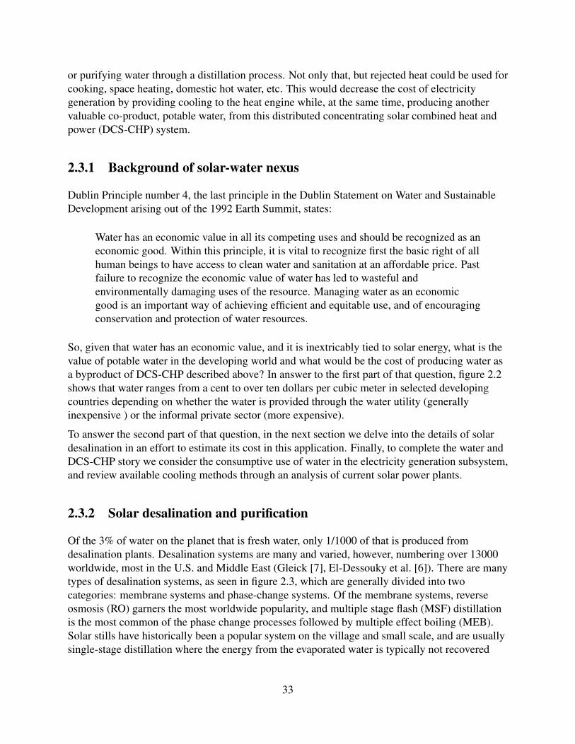
So, given that water has an economic value, and it is inextricably tied to solar energy, what is thevalue of potable water in the developing world and what would be the cost of producing water asa byproduct of DCS-CHP described above? In answer to the first part of that question, figure 2.2shows that water ranges from a cent to over ten dollars per cubic meter in selected developingcountries depending on whether the water is provided through the water utility (generallyinexpensive ) or the informal private sector (more expensive).
To answer the second part of that question, in the next section we delve into the details of solardesalination in an effort to estimate its cost in this application. Finally, to complete the water andDCS-CHP story we consider the consumptive use of water in the electricity generation subsystem,and review available cooling methods through an analysis of current solar power plants.
2.3.2 Solar desalination and purification
Of the 3% of water on the planet that is fresh water, only 1/1000 of that is produced fromdesalination plants. Desalination systems are many and varied, however, numbering over 13000worldwide, most in the U.S. and Middle East (Gleick [7], El-Dessouky et al. [6]). There are manytypes of desalination systems, as seen in figure 2.3, which are generally divided into twocategories: membrane systems and phase-change systems. Of the membrane systems, reverseosmosis (RO) garners the most worldwide popularity, and multiple stage flash (MSF) distillationis the most common of the phase change processes followed by multiple effect boiling (MEB).Solar stills have historically been a popular system on the village and small scale, and are usuallysingle-stage distillation where the energy from the evaporated water is typically not recovered
33
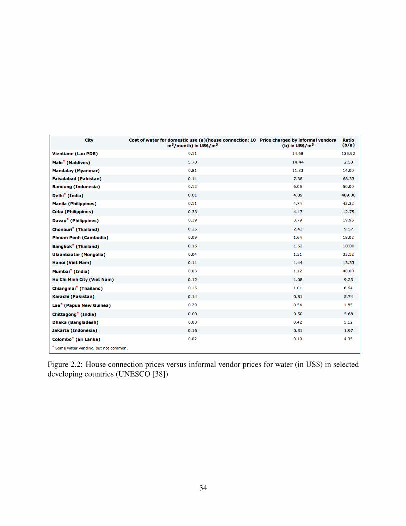
Figure 2.2: House connection prices versus informal vendor prices for water (in US$) in selecteddeveloping countries (UNESCO [38])
34
Figure 2.3: Desalination processes (Kalogirou [13])
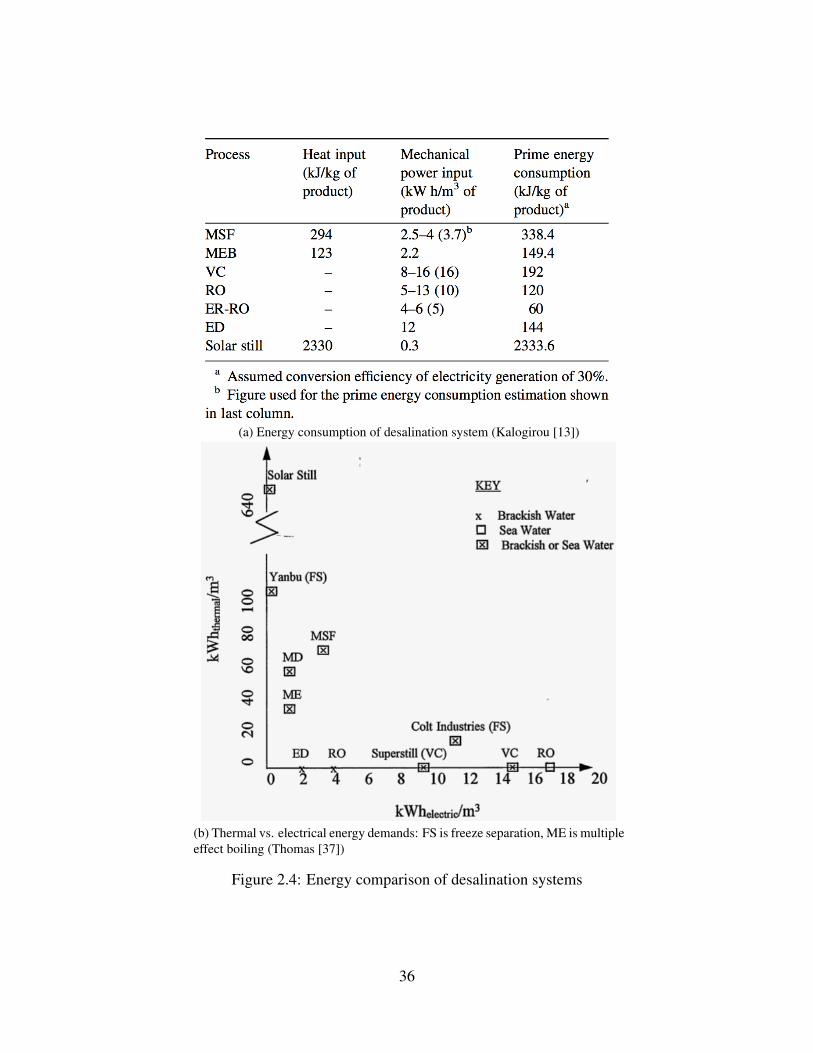
thus leading to lower overall system efficiency. MSF systems tend to be larger (on the scale of1000 to 100,000 m3/day), but MEB systems have been designed in rugged varieties suitable todeployment in small villages under less controlled and less skilled operation (Thomas[37], Kalogirou [11]).
Looking at the energy required for each type of plant can help guide the selection of thetechnologically and economically optimum desalination system to run off the waste heat of adistributed concentrating solar combined heat and power system (DCS-CHP). Figure 2.4 showsthe required energy for different desalination systems.
It is interesting to note that membrane systems consume the least energy, yet all that energy mustbe mechanical work, making them an inappropriate technology to use with a system likeDCS-CHP where thermal energy is abundant and thermal to electrical/mechanical energyconversion efficiency is low. The fact that the most abundant energy available from a DCS-CHPsystem is moderate grade heat (at around 370K), rules out the use of vapor compression, reverseosmosis, and electrodialysis as the optimum choice for desalination. Of the remaining choices, itis important to look at the method of operation of the system to further narrow down the selection.Kalogirou has published several papers on the selection of optimal desalination systems for solar(Kalogirou [13, 11]). He concludes that the MEB process with a multiple effect stacked (MES)evaporator is the most appropriate for solar, a schematic of which is shown in figure 2.5.
An MES with a DCS-CHP system would function like this:
1. Low pressure steam (generated from the condenser of the Rankine cycle) will enter into atube array in the 1st effect as the feed-water is sprayed down from above.
2. The steam will condense while causing the feed-water (at lower pressure) to evaporate onthe outside of the tubes. The condensate that forms inside the tubes will become part of the
35
(a) Energy consumption of desalination system (Kalogirou [13])
(b) Thermal vs. electrical energy demands: FS is freeze separation, ME is multipleeffect boiling (Thomas [37])
Figure 2.4: Energy comparison of desalination systems
36
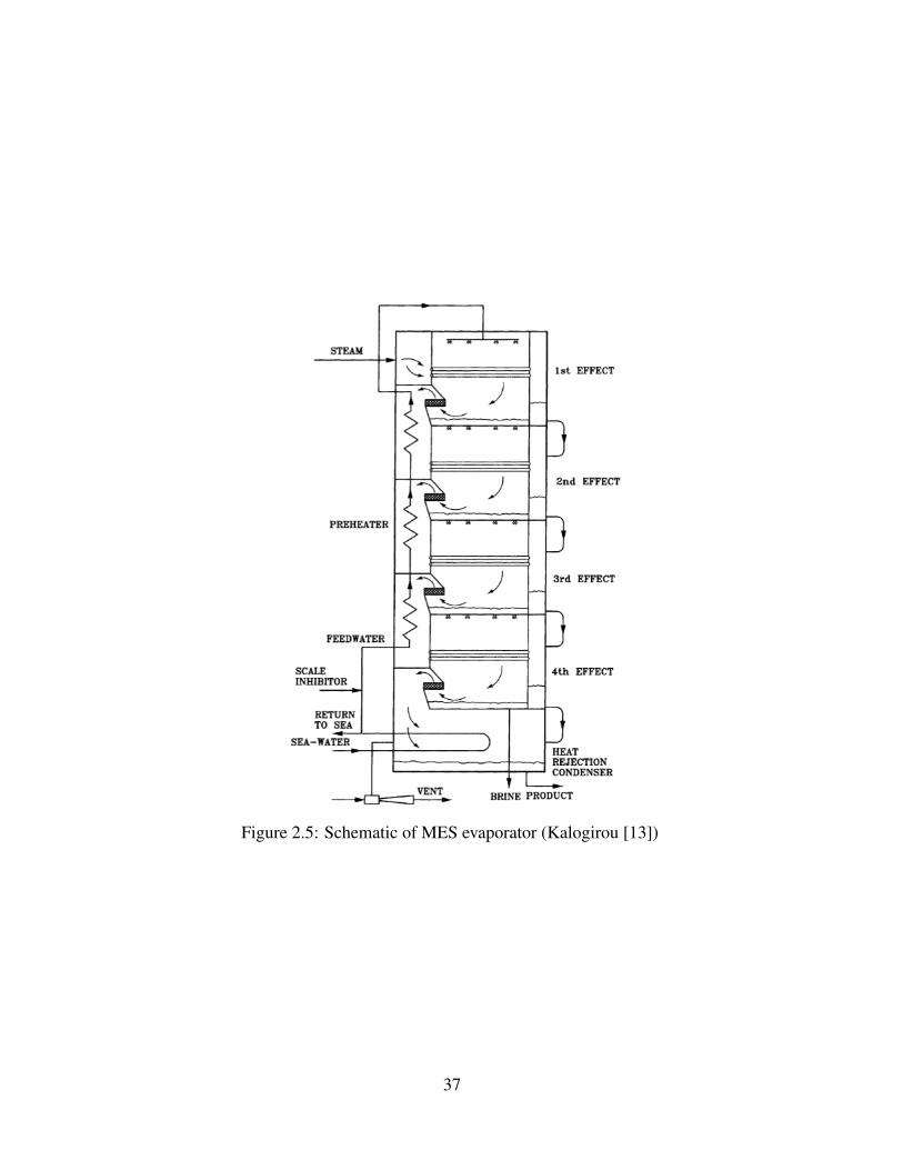
Figure 2.5: Schematic of MES evaporator (Kalogirou [13])
37

product water while the evaporate from the outside of the tubes will flow into the nexteffect.
3. The feed-water that doesn’t evaporate drips down into a pool in the first effect and goesthrough a nozzle dropping the pressure and falling onto the tubes of the 2nd effect wherethe steam inside the tubes (the evaporate from the first effect) again causes vaporization ofthe now slightly more saturated feed-water solution.
4. This effect continues and at each stage the condensate coming from the tubes becomes partof the product until the last stage where the unheated feed-water loop condenses the lastevaporate to add to the final product while the brine from the last stage is removed.
5. At the same time steps 1-4 are occurring the feed-water is being heated sequentially, as it ispiped up from the 4th effect to the 1st, gradually warming as it goes until it is sprayed ontothe tubes of the 1st effect as described in step 1.
The choice of a MEB distillation system is synergistic with the DCS-CHP concept because thetemperatures needed for a MEB are in the 340-370K range, which exactly matches thecondensation temperature for the steam Rankine system. Because MEB is an indirect solardistillation process (i.e. the sunlight would not be directly evaporating the water to be purified)the condenser will effectively act to transfer energy from the condensing working fluid of theRankine subsystem to the feed-water of the desalination/purification system as illustrated in thesystem schematic of figure 2.6.
Kalogirou surveyed dozens of solar MEB systems installed worldwide (results shown in figure2.7) and concluded the following benefits of MEB systems for solar desalination:
• Like any boiling process, MEB inherently removes salinity, manganese, fluoride, heavymetals, microbiological contamination and pesticide/herbicide residues.
• MEB is the cheapest of all indirect collection systems (See figure 2.7).
• MEB is robust in that it does not require highly trained operators to keep it running safely.There are no complicated additives to use, nor, as in RO, can misoperation cause damage tothe membrane allowing contaminated water to be passed through.
• MEB is stable for varying energy supply from 0 to 100% of capacity, so it is uniquelysuited for fluctuating solar insolation levels.
• Very small amounts of descaling agent can be used in seawater desalination as the system iseffectively a once-through process, and the feed-water is at its lowest impurityconcentrations a the highest temperature.
• The total cost of MEB with solar thermal is less than RO with photovoltaics because of thehigh cost of photovoltaic electricity.
• Improved energy efficiency is possible because the brine is not heated above its boilingpoint, leading to less irreversibility (i.e. less entropy generation).
38
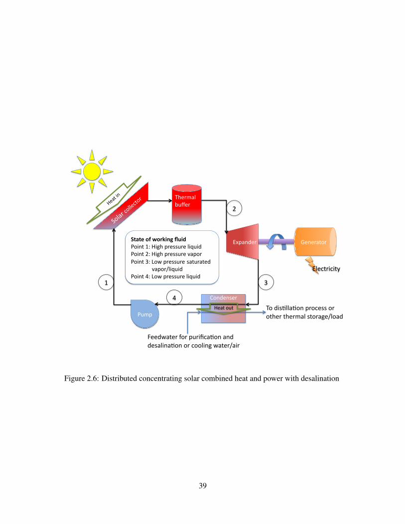
!"#$%&'() *'%'($+,()
!-'.+(/./+0)
123#)
45'(3$-)
627'()
8,%&'%9'()
:''&;$+'()<,()#2(/=.$>,%)$%&)
&'9$-/%$>,%),().,,-/%?);$+'(@$/()
4,)&/9>--$>,%)#(,.'99),()
,+5'()+5'(3$-)9+,($?'@-,$&)
A)
B)
C)
D)
!"#"$%&'%(&)*+,-%./+0%
1,/%+)AE)F/?5)#('992(')-/G2/&)
1,/%+)BE)F/?5)#('992(')H$#,()
1,/%+)CE)I,;)#('992('))9$+2($+'&)
))))))H$#,(@-/G2/&)
1,/%+)DE)I,;)#('992(')-/G2/&)
F'$+),2+)
Figure 2.6: Distributed concentrating solar combined heat and power with desalination
39
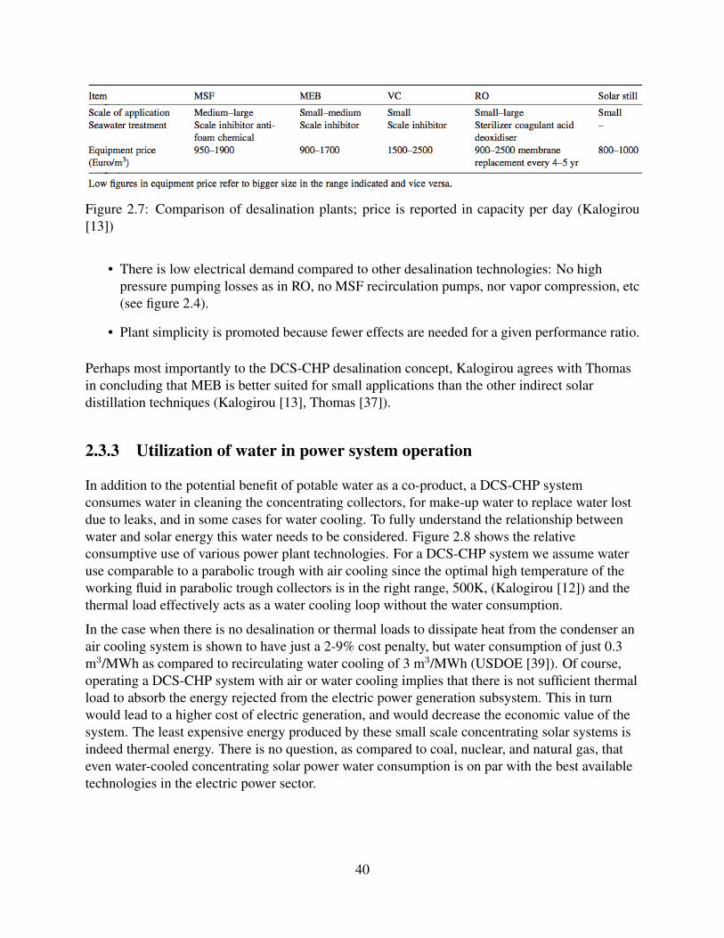
Figure 2.7: Comparison of desalination plants; price is reported in capacity per day (Kalogirou[13])
• There is low electrical demand compared to other desalination technologies: No highpressure pumping losses as in RO, no MSF recirculation pumps, nor vapor compression, etc(see figure 2.4).
• Plant simplicity is promoted because fewer effects are needed for a given performance ratio.
Perhaps most importantly to the DCS-CHP desalination concept, Kalogirou agrees with Thomasin concluding that MEB is better suited for small applications than the other indirect solardistillation techniques (Kalogirou [13], Thomas [37]).
2.3.3 Utilization of water in power system operation
In addition to the potential benefit of potable water as a co-product, a DCS-CHP systemconsumes water in cleaning the concentrating collectors, for make-up water to replace water lostdue to leaks, and in some cases for water cooling. To fully understand the relationship betweenwater and solar energy this water needs to be considered. Figure 2.8 shows the relativeconsumptive use of various power plant technologies. For a DCS-CHP system we assume wateruse comparable to a parabolic trough with air cooling since the optimal high temperature of theworking fluid in parabolic trough collectors is in the right range, 500K, (Kalogirou [12]) and thethermal load effectively acts as a water cooling loop without the water consumption.
In the case when there is no desalination or thermal loads to dissipate heat from the condenser anair cooling system is shown to have just a 2-9% cost penalty, but water consumption of just 0.3m3/MWh as compared to recirculating water cooling of 3 m3/MWh (USDOE [39]). Of course,operating a DCS-CHP system with air or water cooling implies that there is not sufficient thermalload to absorb the energy rejected from the electric power generation subsystem. This in turnwould lead to a higher cost of electric generation, and would decrease the economic value of thesystem. The least expensive energy produced by these small scale concentrating solar systems isindeed thermal energy. There is no question, as compared to coal, nuclear, and natural gas, thateven water-cooled concentrating solar power water consumption is on par with the best availabletechnologies in the electric power sector.
40
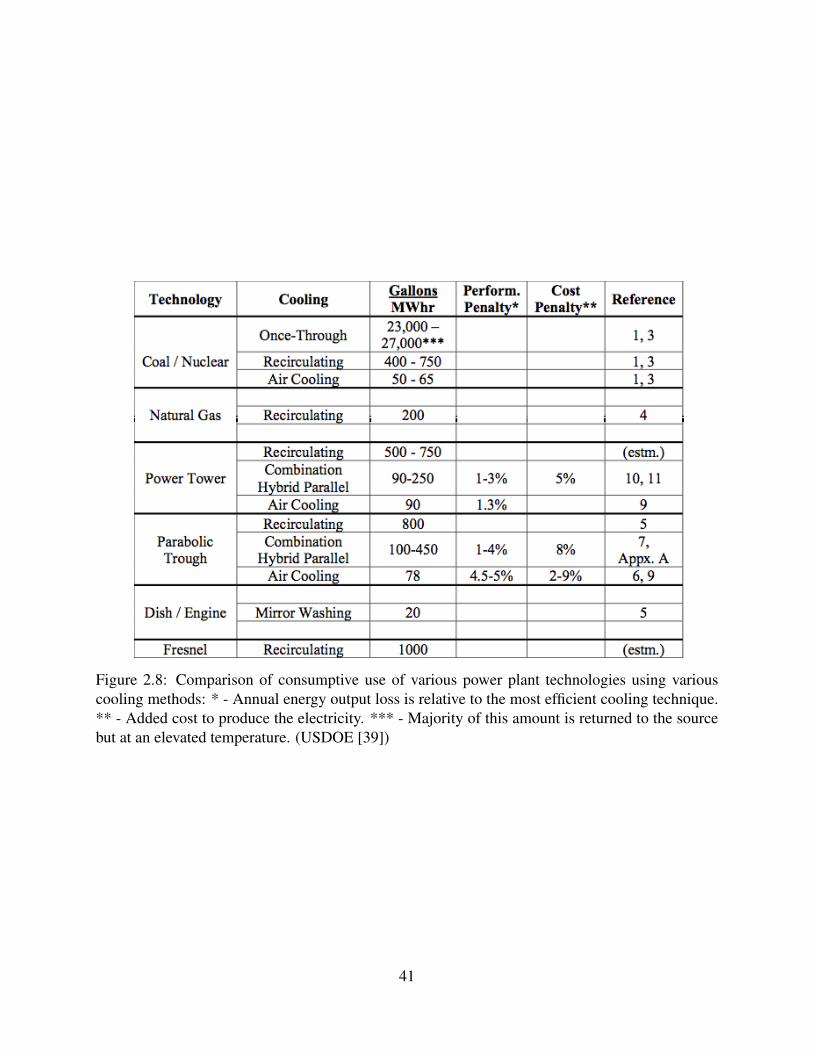
Figure 2.8: Comparison of consumptive use of various power plant technologies using variouscooling methods: * - Annual energy output loss is relative to the most efficient cooling technique.** - Added cost to produce the electricity. *** - Majority of this amount is returned to the sourcebut at an elevated temperature. (USDOE [39])
41
2.3.4 Solar desalination economics
Thomas reviewed the costs of various desalination systems for the village scale and states thatsolar thermal MEB has a levelized cost of $0.70-$4.00/m3 with the low end referenced to a capitalcost of $1000/m3 of capacity on a daily basis (Thomas [37]). We would expect system cost to bein this range for a DCS-CHP system where the solar field cost is split between the electricalgeneration and the solar thermal generation as described by Norwood et al. (Norwood et al. [23]).With a predicted levelized solar thermal cost of $0.03/kWh, this leads to a limiting estimate of thecost of a solar still at $21/m3 (based on the thermodynamic minimum energy, 2800 J/g, toevaporate water from ambient temperature). Since the multiple effect evaporator has about 1/15ththe energy use of a solar still we would predict a cost of $1.40/m3 for an indirect solar MEB asdescribed in this paper. El-Dessouky cites the cost of a low-temperature MEB at $0.45/m3 fromfossil fuel sources, or about one third the predicted cost from DCS-CHP with desalination of$1.40/m3. This is at the high end of the household cost of water for selected Asian developingcountries as presented in figure 2.2, and is competitive with the informal sector for about half ofthose countries.
2.4 Conclusions
The life cycle analysis presented in the first part of this chapter affirms that a solar Rankine CHPsystem can be cost effective and directly competitive with other fossil and renewable energyproduction methods in small scale. The cost and environmental benefits of this system could beimproved by further refinements in both trough and dish collector systems, and by continueddevelopment of a low-cost expander like the Katrix rotary lobe expander for use with steam as theworking fluid. LCA economics of this specific DCS-CHP system agree well with the generic casestudy of Chapter 1. The results presented here predict levelized costs of $0.25/kWh electricityand $0.03/kWh thermal, for a system with a life-cycle global warming potential of ~80gCO2eq/kWh of electricity and ~10 gCO2eq/kWh thermal.
Based on the reasonable economics shown for air-cooling, and the fact that any combined heatand power system reduces the need for cooling while at the same time boosting the overall solarefficiency of the system, DCS-CHP does rate among the best electric power generation systems interms of minimization of water use in the maintenance and operation of the plant. Additionally,the LCA of the embodied water in the manufacture of a concentrating solar system, which usesprimarily common metals and glass in simple manufacturing processes, promises to beinsignificant, (on the order of 0.03 m3/MWh) even as compared to the modest water use inoperation (Montgomery [19]) .
The outlook for water desalination coupled with distributed concentrating solar combined heatand power is another story. Based on the economics described in the last section, waterdesalination with DCS-CHP would be economical and practical only in areas where water is veryscarce or moderately expensive, primarily available through the informal sector, and wherecontaminated, or salt water is easily available as feed-water. Additionally, the cost of fossil fuels
42

would have to be greater than DCS-CHP solar energy for the economics to favor solardesalination in the first place. It is also interesting to note that $0.40-$1.90/m3 is the range ofwater prices in the developed world (UNESCO [38]), so DCS-CHP desalination systems, at apredicted cost $1.40/m3, would be an economical solution there under some conditions. Ofcourse, in most developed countries the cost effective option to meet water scarcity problems is toincrease water end-use efficiency and forgo energy-intensive supply side augmentation such asdesalination altogether.
43

Chapter 3
Testing of the Katrix Rotary Lobe Expander
44
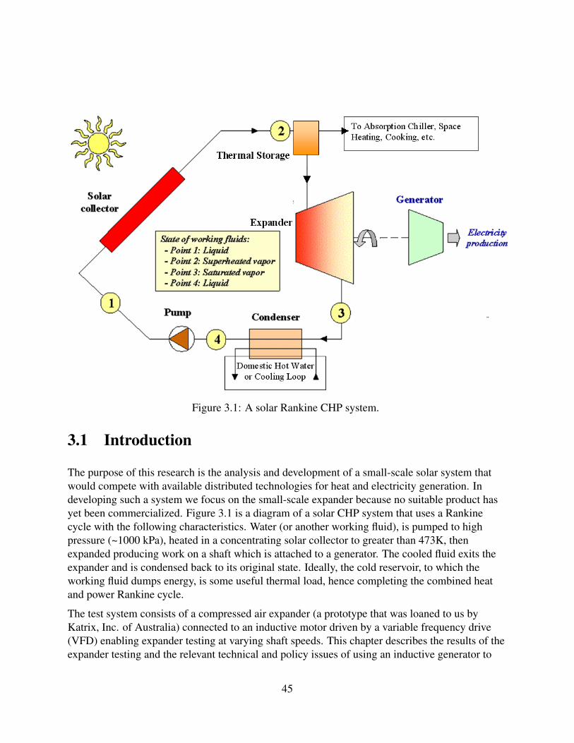
Figure 3.1: A solar Rankine CHP system.
3.1 Introduction
The purpose of this research is the analysis and development of a small-scale solar system thatwould compete with available distributed technologies for heat and electricity generation. Indeveloping such a system we focus on the small-scale expander because no suitable product hasyet been commercialized. Figure 3.1 is a diagram of a solar CHP system that uses a Rankinecycle with the following characteristics. Water (or another working fluid), is pumped to highpressure (~1000 kPa), heated in a concentrating solar collector to greater than 473K, thenexpanded producing work on a shaft which is attached to a generator. The cooled fluid exits theexpander and is condensed back to its original state. Ideally, the cold reservoir, to which theworking fluid dumps energy, is some useful thermal load, hence completing the combined heatand power Rankine cycle.
The test system consists of a compressed air expander (a prototype that was loaned to us byKatrix, Inc. of Australia) connected to an inductive motor driven by a variable frequency drive(VFD) enabling expander testing at varying shaft speeds. This chapter describes the results of theexpander testing and the relevant technical and policy issues of using an inductive generator to
45

regenerate electricity on UC Berkeley campus. I describe the test procedure, discuss gridharmonic analysis of my test setup (per IEEE 519), and describe the Pacific Gas and Electric Rule21 policy issues to small inductive motor renewable technology. I conclude that small inductivemotor power generators are not, at this time, allowable on PG&E’s grid without going throughrigorous, costly, and time consuming certification and engineering reviews according to Rule 21.Although harmonic distortion is within required limits and, being powered by an electriccompressor, this test setup produces no net electrical energy, I nonetheless dissipate theregenerated electric energy to a bank of dynamic braking resistors to satisfy the campus EH&Sand physical plant engineers’ requirements of compliance with Rule 21. Results of the expandertesting are a qualified success. Although the expander does not complete testing due to an internalfailure, the isentropic efficiency (80-95%) and pressure ratio (6-11) at the tested speeds isimpressive for a device this small and simple. Future refinements could lead to a new class ofexpanders with unequaled low-cost and high-performance for use in solar combined heat andpower.
46
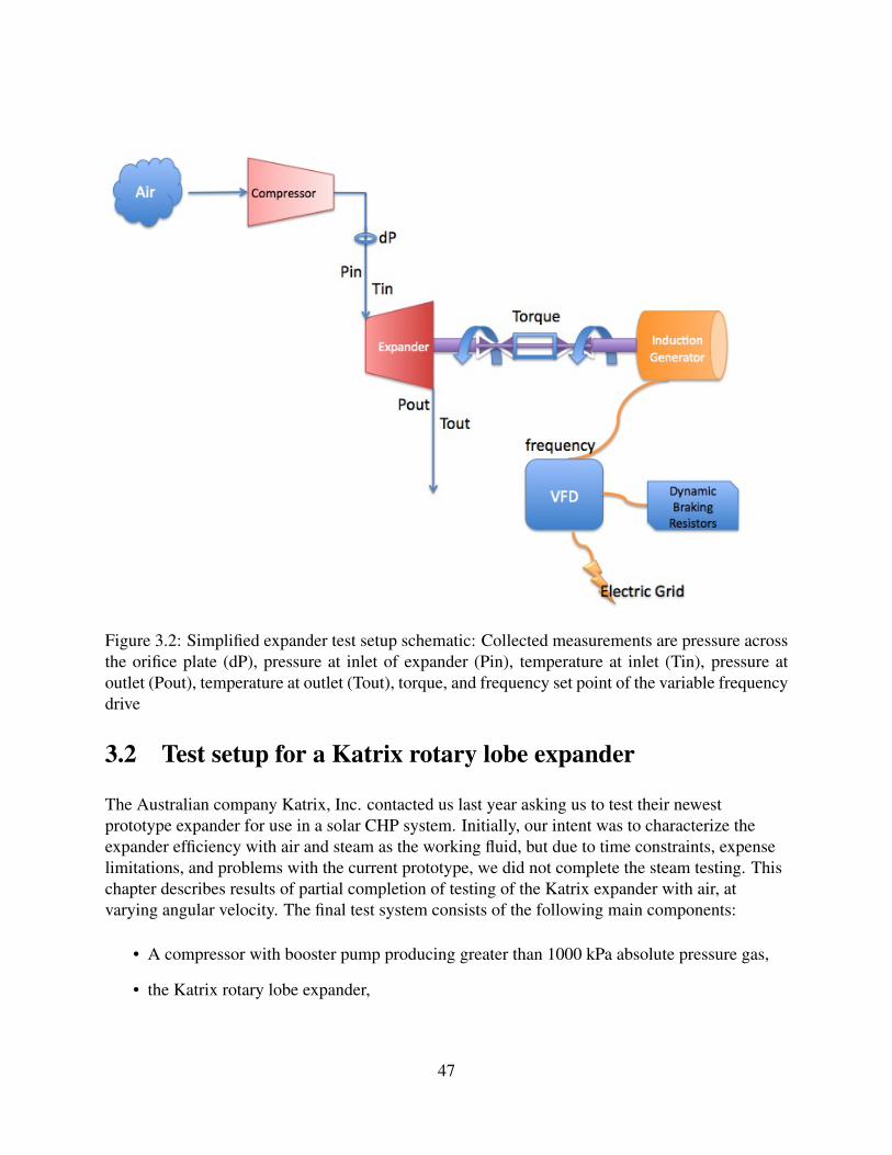
Figure 3.2: Simplified expander test setup schematic: Collected measurements are pressure acrossthe orifice plate (dP), pressure at inlet of expander (Pin), temperature at inlet (Tin), pressure atoutlet (Pout), temperature at outlet (Tout), torque, and frequency set point of the variable frequencydrive
3.2 Test setup for a Katrix rotary lobe expander
The Australian company Katrix, Inc. contacted us last year asking us to test their newestprototype expander for use in a solar CHP system. Initially, our intent was to characterize theexpander efficiency with air and steam as the working fluid, but due to time constraints, expenselimitations, and problems with the current prototype, we did not complete the steam testing. Thischapter describes results of partial completion of testing of the Katrix expander with air, atvarying angular velocity. The final test system consists of the following main components:
• A compressor with booster pump producing greater than 1000 kPa absolute pressure gas,
• the Katrix rotary lobe expander,
47
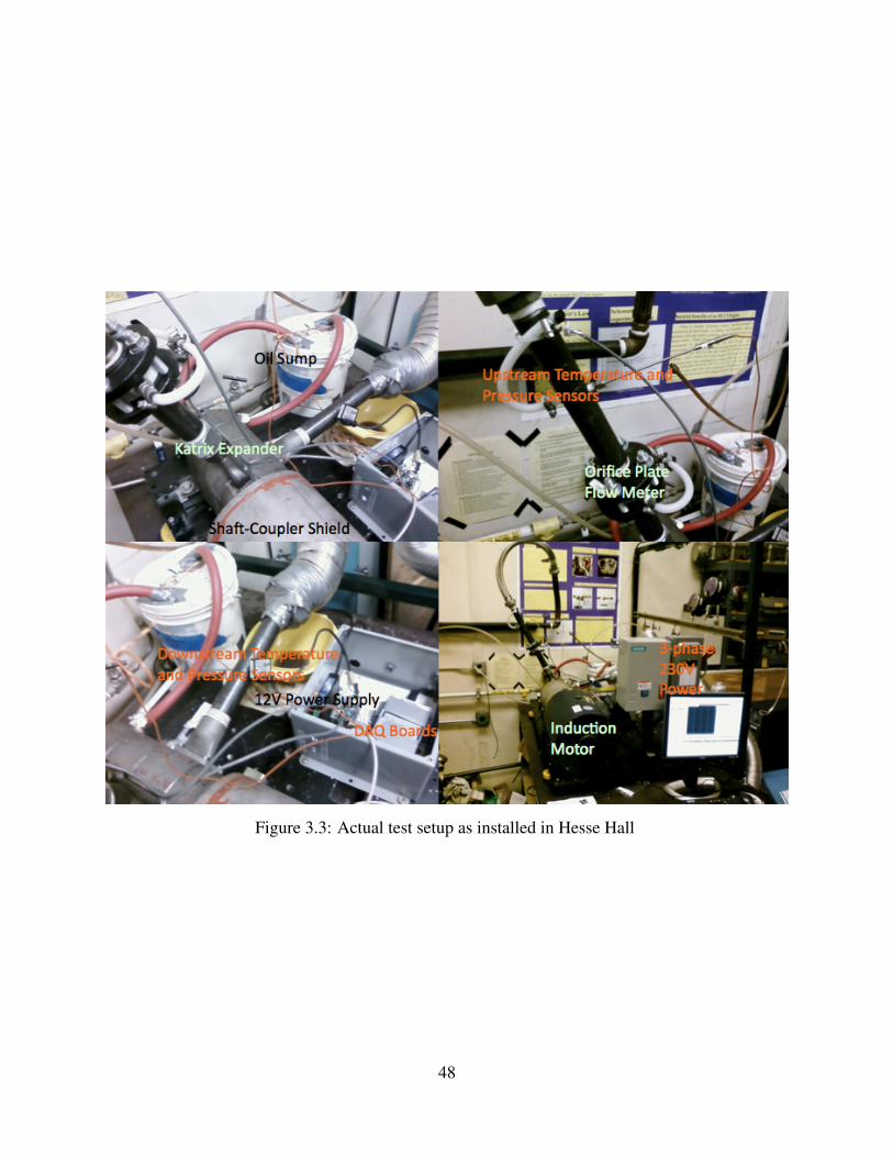
Figure 3.3: Actual test setup as installed in Hesse Hall
48
• upstream and downstream pressure and temperature probes (used to calculate enthalpychange of the working fluid),
• an in-line shaft torque measurement device,
• an upstream orifice plate flow meter with differential pressure sensor and a rotameter ofknown calibration (used to calculate flow rate),
• and a variable frequency drive with dynamic braking resistor pack providing load to theexpander.
Figure 3.2 shows a simplified schematic of the test setup with relevant data measurement points,and figure 3.3 shows actual pictures of the test equipment in the basement of Hesse Hall on theUC Berkeley campus. Appendix A also contains a list of all equipment used in the testing,including the VFD, which is not shown in the pictures.
Experiments follow this operating procedure:
1. Turn on the VFD to the desired frequency set point (in this case 10-60 Hz AC, whichcorresponds to 31-188 rad/sec or 300-1800 rpm) so the electric motor spins theexpander up to the desired angular velocity.
2. Turn on the compressed air supply so the expander powers the shaft to the electricmotor and any excess regenerated electrical power is dissipated in a resistor bankconnected to the VFD.
3. After the system runs for 10-15 minutes to “warm up” (i.e. reach steady statetemperature at expander inlet and outlet) start data acquisition on the upstream anddownstream pressure and temperature of the working fluid, torque on the shaft, anddifferential pressure across the orifice plate flow meter.
4. After a 10-15 minute data collection period, stop data acquisition and increase theVFD frequency set point by 5Hz.
5. Repeat steps 3 and 4 until the VFD frequency reaches 60Hz (the limits of the VFDand motor) being sure to wait for steady state operation before doing data acquisitionat each speed.
6. Shut off the compressed air and turn off the VFD, in that order.
7. Find a 300 second period of recorded data with fairly steady characteristics ofupstream pressure and temperature and calculate isentropic efficiency of theexpander.
Matlab and Engineering Equation Solver software is used for post-processing of the experimentaldata. Using the two independent state variables of measured temperature and pressure, fluid inletand outlet states can be fully determined. The specific enthalpy drop of the working fluid across
49
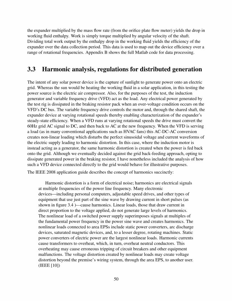
the expander multiplied by the mass flow rate (from the orifice plate flow meter) yields the drop inworking fluid enthalpy. Work is simply torque multiplied by angular velocity of the shaft.Dividing total work output by the enthalpy drop in the working fluid yields the efficiency of theexpander over the data collection period. This data is used to map out the device efficiency over arange of rotational frequencies. Appendix B shows the full Matlab code for data processing.
3.3 Harmonic analysis, regulations for distributed generation
The intent of any solar power device is the capture of sunlight to generate power onto an electricgrid. Whereas the sun would be heating the working fluid in a solar application, in this testing thepower source is the electric air compressor. Also, for the purposes of the test, the inductiongenerator and variable frequency drive (VFD) act as the load. Any electrical power generated bythe test rig is dissipated in the braking resistor pack when an over-voltage condition occurs on theVFD’s DC bus. The variable frequency drive controls the motor and, through the shared shaft, theexpander device at varying rotational speeds thereby enabling characterization of the expander’ssteady-state efficiency. When a VFD runs at varying rotational speeds the drive must convert the60Hz grid AC signal to DC, and then back to AC at the new frequency. When the VFD is servinga load (as in many conventional applications such as HVAC fans) this AC-DC-AC conversioncreates non-linear loading which disturbs the perfect sinusoidal voltage and current waveforms ofthe electric supply leading to harmonic distortion. In this case, where the induction motor isinstead acting as a generator, the same harmonic distortion is created when the power is fed backonto the grid. Although we eventually decided against the grid back-feeding approach, opting todissipate generated power in the braking resistor, I have nonetheless included the analysis of howsuch a VFD device connected directly to the grid would behave for illustrative purposes.
The IEEE 2008 application guide describes the concept of harmonics succinctly:
Harmonic distortion is a form of electrical noise; harmonics are electrical signalsat multiple frequencies of the power line frequency. Many electronicdevices—including personal computers, adjustable speed drives, and other types ofequipment that use just part of the sine wave by drawing current in short pulses (asshown in figure 3.4 )—cause harmonics. Linear loads, those that draw current indirect proportion to the voltage applied, do not generate large levels of harmonics.The nonlinear load of a switched power supply superimposes signals at multiples ofthe fundamental power frequency in the power sine wave and creates harmonics. Thenonlinear loads connected to area EPSs include static power converters, arc dischargedevices, saturated magnetic devices, and, to a lesser degree, rotating machines. Staticpower converters of electric power are the largest nonlinear loads. Harmonic currentscause transformers to overheat, which, in turn, overheat neutral conductors. Thisoverheating may cause erroneous tripping of circuit breakers and other equipmentmalfunctions. The voltage distortion created by nonlinear loads may create voltagedistortion beyond the premise’s wiring system, through the area EPS, to another user.(IEEE [10])
50
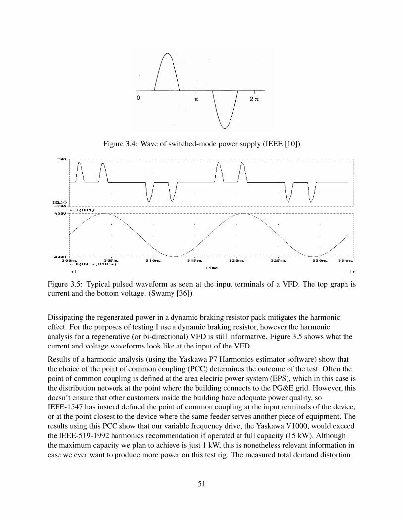
Figure 3.4: Wave of switched-mode power supply (IEEE [10])
Figure 3.5: Typical pulsed waveform as seen at the input terminals of a VFD. The top graph iscurrent and the bottom voltage. (Swamy [36])
Dissipating the regenerated power in a dynamic braking resistor pack mitigates the harmoniceffect. For the purposes of testing I use a dynamic braking resistor, however the harmonicanalysis for a regenerative (or bi-directional) VFD is still informative. Figure 3.5 shows what thecurrent and voltage waveforms look like at the input of the VFD.
Results of a harmonic analysis (using the Yaskawa P7 Harmonics estimator software) show thatthe choice of the point of common coupling (PCC) determines the outcome of the test. Often thepoint of common coupling is defined at the area electric power system (EPS), which in this case isthe distribution network at the point where the building connects to the PG&E grid. However, thisdoesn’t ensure that other customers inside the building have adequate power quality, soIEEE-1547 has instead defined the point of common coupling at the input terminals of the device,or at the point closest to the device where the same feeder serves another piece of equipment. Theresults using this PCC show that our variable frequency drive, the Yaskawa V1000, would exceedthe IEEE-519-1992 harmonics recommendation if operated at full capacity (15 kW). Althoughthe maximum capacity we plan to achieve is just 1 kW, this is nonetheless relevant information incase we ever want to produce more power on this test rig. The measured total demand distortion
51
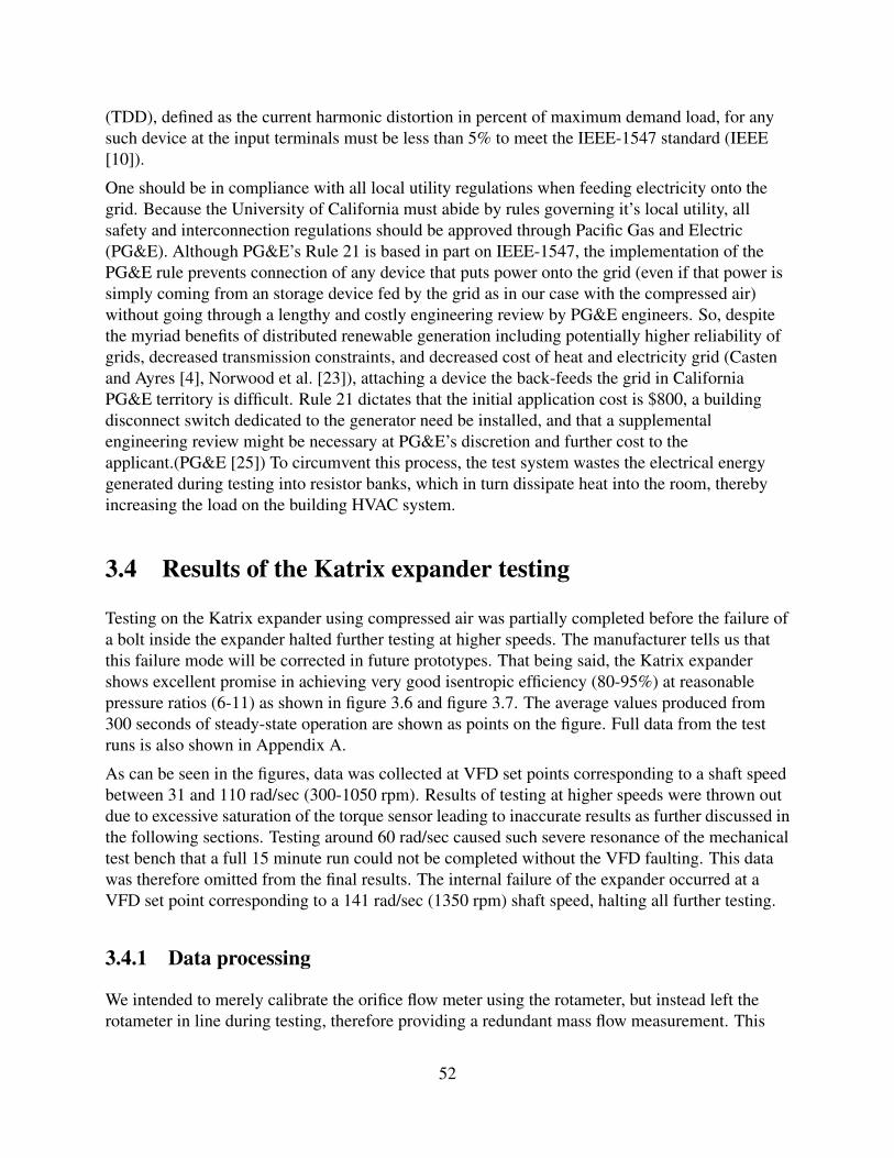
(TDD), defined as the current harmonic distortion in percent of maximum demand load, for anysuch device at the input terminals must be less than 5% to meet the IEEE-1547 standard (IEEE[10]).
One should be in compliance with all local utility regulations when feeding electricity onto thegrid. Because the University of California must abide by rules governing it’s local utility, allsafety and interconnection regulations should be approved through Pacific Gas and Electric(PG&E). Although PG&E’s Rule 21 is based in part on IEEE-1547, the implementation of thePG&E rule prevents connection of any device that puts power onto the grid (even if that power issimply coming from an storage device fed by the grid as in our case with the compressed air)without going through a lengthy and costly engineering review by PG&E engineers. So, despitethe myriad benefits of distributed renewable generation including potentially higher reliability ofgrids, decreased transmission constraints, and decreased cost of heat and electricity grid (Castenand Ayres [4], Norwood et al. [23]), attaching a device the back-feeds the grid in CaliforniaPG&E territory is difficult. Rule 21 dictates that the initial application cost is $800, a buildingdisconnect switch dedicated to the generator need be installed, and that a supplementalengineering review might be necessary at PG&E’s discretion and further cost to theapplicant.(PG&E [25]) To circumvent this process, the test system wastes the electrical energygenerated during testing into resistor banks, which in turn dissipate heat into the room, therebyincreasing the load on the building HVAC system.
3.4 Results of the Katrix expander testing
Testing on the Katrix expander using compressed air was partially completed before the failure ofa bolt inside the expander halted further testing at higher speeds. The manufacturer tells us thatthis failure mode will be corrected in future prototypes. That being said, the Katrix expandershows excellent promise in achieving very good isentropic efficiency (80-95%) at reasonablepressure ratios (6-11) as shown in figure 3.6 and figure 3.7. The average values produced from300 seconds of steady-state operation are shown as points on the figure. Full data from the testruns is also shown in Appendix A.
As can be seen in the figures, data was collected at VFD set points corresponding to a shaft speedbetween 31 and 110 rad/sec (300-1050 rpm). Results of testing at higher speeds were thrown outdue to excessive saturation of the torque sensor leading to inaccurate results as further discussed inthe following sections. Testing around 60 rad/sec caused such severe resonance of the mechanicaltest bench that a full 15 minute run could not be completed without the VFD faulting. This datawas therefore omitted from the final results. The internal failure of the expander occurred at aVFD set point corresponding to a 141 rad/sec (1350 rpm) shaft speed, halting all further testing.
3.4.1 Data processing
We intended to merely calibrate the orifice flow meter using the rotameter, but instead left therotameter in line during testing, therefore providing a redundant mass flow measurement. This
52
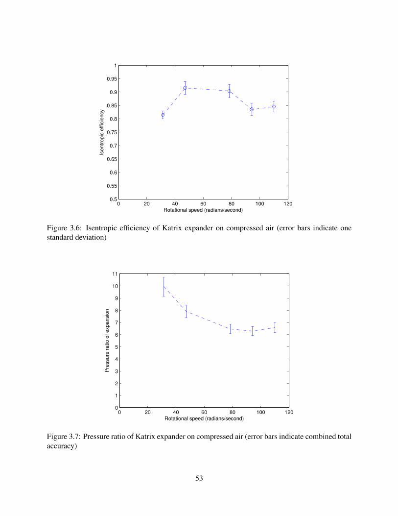
0 20 40 60 80 100 1200.5
0.55
0.6
0.65
0.7
0.75
0.8
0.85
0.9
0.95
1
Ise
ntr
opic
effic
iency
Rotational speed (radians/second)
Figure 3.6: Isentropic efficiency of Katrix expander on compressed air (error bars indicate onestandard deviation)
0 20 40 60 80 100 1200
1
2
3
4
5
6
7
8
9
10
11
Pre
ssu
re r
atio
of exp
ansi
on
Rotational speed (radians/second)
Figure 3.7: Pressure ratio of Katrix expander on compressed air (error bars indicate combined totalaccuracy)
53
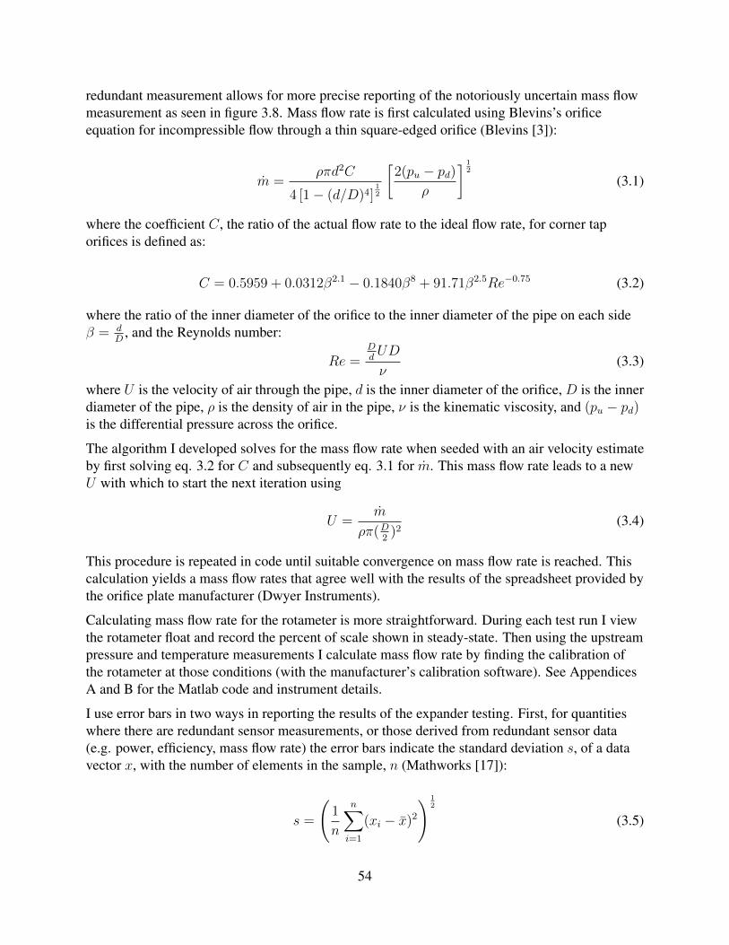
redundant measurement allows for more precise reporting of the notoriously uncertain mass flowmeasurement as seen in figure 3.8. Mass flow rate is first calculated using Blevins’s orificeequation for incompressible flow through a thin square-edged orifice (Blevins [3]):
m ="#d2C
4 [1! (d/D)4]12
)2(pu ! pd)
"
* 12
(3.1)
where the coefficient C, the ratio of the actual flow rate to the ideal flow rate, for corner taporifices is defined as:
C = 0.5959 + 0.0312$2.1 ! 0.1840$8 + 91.71$2.5Re"0.75 (3.2)
where the ratio of the inner diameter of the orifice to the inner diameter of the pipe on each side$ = d
D , and the Reynolds number:
Re =Dd UD
%(3.3)
where U is the velocity of air through the pipe, d is the inner diameter of the orifice, D is the innerdiameter of the pipe, " is the density of air in the pipe, % is the kinematic viscosity, and (pu ! pd)is the differential pressure across the orifice.
The algorithm I developed solves for the mass flow rate when seeded with an air velocity estimateby first solving eq. 3.2 for C and subsequently eq. 3.1 for m. This mass flow rate leads to a newU with which to start the next iteration using
U =m
"#(D2 )2
(3.4)
This procedure is repeated in code until suitable convergence on mass flow rate is reached. Thiscalculation yields a mass flow rates that agree well with the results of the spreadsheet provided bythe orifice plate manufacturer (Dwyer Instruments).
Calculating mass flow rate for the rotameter is more straightforward. During each test run I viewthe rotameter float and record the percent of scale shown in steady-state. Then using the upstreampressure and temperature measurements I calculate mass flow rate by finding the calibration ofthe rotameter at those conditions (with the manufacturer’s calibration software). See AppendicesA and B for the Matlab code and instrument details.
I use error bars in two ways in reporting the results of the expander testing. First, for quantitieswhere there are redundant sensor measurements, or those derived from redundant sensor data(e.g. power, efficiency, mass flow rate) the error bars indicate the standard deviation s, of a datavector x, with the number of elements in the sample, n (Mathworks [17]):
s =
+1
n
n,
i=1
(xi ! x)2- 1
2
(3.5)
54

0 20 40 60 80 100 1200
0.002
0.004
0.006
0.008
0.01
0.012
0.014
0.016
0.018
0.02
Mass
flo
w r
ate
of air in
to e
xpander
(kg/s
eco
nd)
Rotational speed (radians/second)
Figure 3.8: Mass flow rate of air through expander (error bars indicate one standard deviation)
where
x =1
n
n,
i=1
xi (3.6)
This calculation assumes that all derived measurements are truly independent, but is not strictlyaccurate for derived measurements such as fluid enthalpy and efficiency because in this test setupthere are independent/redundant mass flow measurements, but some single temperature andpressure measurements. Since temperature and pressure measurements are comparatively morerobust than mass flow rate measurement, the resulting underestimate of the standard deviation isignored. Because the accuracy of the data acquisition hardware is so high, any data acquisitionerror is also omitted from the error bars. The second way in which error bars are reported here arefor those sensors that have manufacturer published accuracy (e.g. pressure, temperature, rotationalspeed, and torque measurements). These error bars report total combined accuracy or tolerancefor these types of measurements. Derived values (such as pressure ratio, torque, mechanicalpower) have error bars derived from the relative contribution of accuracy from each sensor. Thedetails of these combined error calculations are available in the full Matlab code of Appendix B.
Figure 3.10 and figure 3.9 show temperature and pressure measurements of air entering andexiting the expander are 310K, 10 bar, and 273K, 1 bar respectively with relatively smallvariations at different expander rotational speeds. The enthalpy change of the working fluid asshown in figure 3.11 is calculated from these measured temperature and pressure values using theEngineering Equation Solver software.
55

0 20 40 60 80 100 120250
260
270
280
290
300
310
320
Tem
pera
ture
(K
elv
in)
Rotational speed (radians/second)
Temperature of air at expander inlet
Temperature of air at expander outlet
Figure 3.9: Temperature of air at expander inlet and outlet (error bars indicate combined totalaccuracy)
0 20 40 60 80 100 1200
1
2
3
4
5
6
7
8
9
10
11x 10
5
Pre
ssure
(P
asc
als
)
Rotational speed (radians/second)
Pressure of air at expander inlet
Pressure of air at expander outlet
Figure 3.10: Pressure of air at expander inlet and outlet (error bars indicate combined total accu-racy)
56
0 20 40 60 80 100 1200
100
200
300
400
500
600
700
Pow
er
(Joule
s/se
cond)
Rotational speed (radians/second)
Enthalpy loss of air through expander
Mechanical power generated
Figure 3.11: Enthalpy loss of air through expander, and mechanical power generated (error barsindicate total combined accuracy)
Mechanical power, also shown in figure 3.11, is simply calculated as rotational speed (asregulated by the VFD) multiplied by average torque, shown in figure 3.12.
3.4.2 Torque oscillation
As mentioned in the last section, the measurement of torque on the shaft between the expanderand VFD mysteriously resulted in large periodic oscillations that varied inversely with rotationalspeed as shown in figure 3.13. Figure 3.14 through figure 3.20 show the 300 second oscillatingdifferential pressure (across the orifice plate) and torque data at each rotational speed. Note thatthese speeds are set points of the VFD, as we do not actually measure the speed independently inthis test setup. Mass flow rate is proportional to differential pressure, therefore the orifice plateflow meter data corroborates the oscillating torque data as a real effect. Note that the torqueoscillates so greatly that the expander goes from generating power to absorbing power over thecourse of one period of oscillation. The full data can be found in Appendix A.
A few possibilities as to the cause of the oscillations have been hypothesized and exploredlimitedly:
1. A Helmholtz oscillation occurs in the air intake port or supply line to the expander inletwhere the opening and closing of the passageways into the expander leads to a resonancesimilar to that generated by blowing across the top of a bottle. Initial analysis of thisphenomena indicates that the frequency of the observed torque oscillation is several orders
57
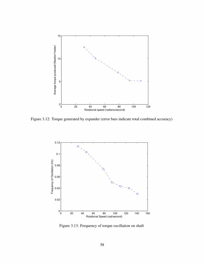
0 20 40 60 80 100 1200
5
10
15
Ave
rage torq
ue p
roduce
d (
New
ton*m
ete
r)
Rotational speed (radians/second)
Figure 3.12: Torque generated by expander (error bars indicate total combined accuracy)
0 20 40 60 80 100 120 140 1600
0.02
0.04
0.06
0.08
0.1
0.12
Fre
quency
of O
scill
atio
n (
Hz)
Rotational Speed (rad/second)
Figure 3.13: Frequency of torque oscillation on shaft
58
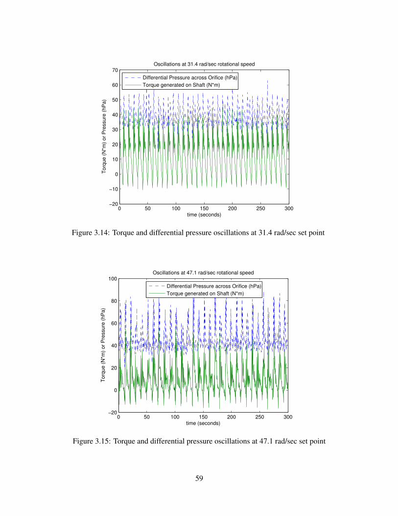
0 50 100 150 200 250 300!20
!10
0
10
20
30
40
50
60
70
Torq
ue (
N*m
) o
r P
ress
ure
(hP
a)
time (seconds)
Oscillations at 31.4 rad/sec rotational speed
Differential Pressure across Orifice (hPa)
Torque generated on Shaft (N*m)
Figure 3.14: Torque and differential pressure oscillations at 31.4 rad/sec set point
0 50 100 150 200 250 300!20
0
20
40
60
80
100
Torq
ue (
N*m
) or
Pre
ssure
(hP
a)
time (seconds)
Oscillations at 47.1 rad/sec rotational speed
Differential Pressure across Orifice (hPa)
Torque generated on Shaft (N*m)
Figure 3.15: Torque and differential pressure oscillations at 47.1 rad/sec set point
59
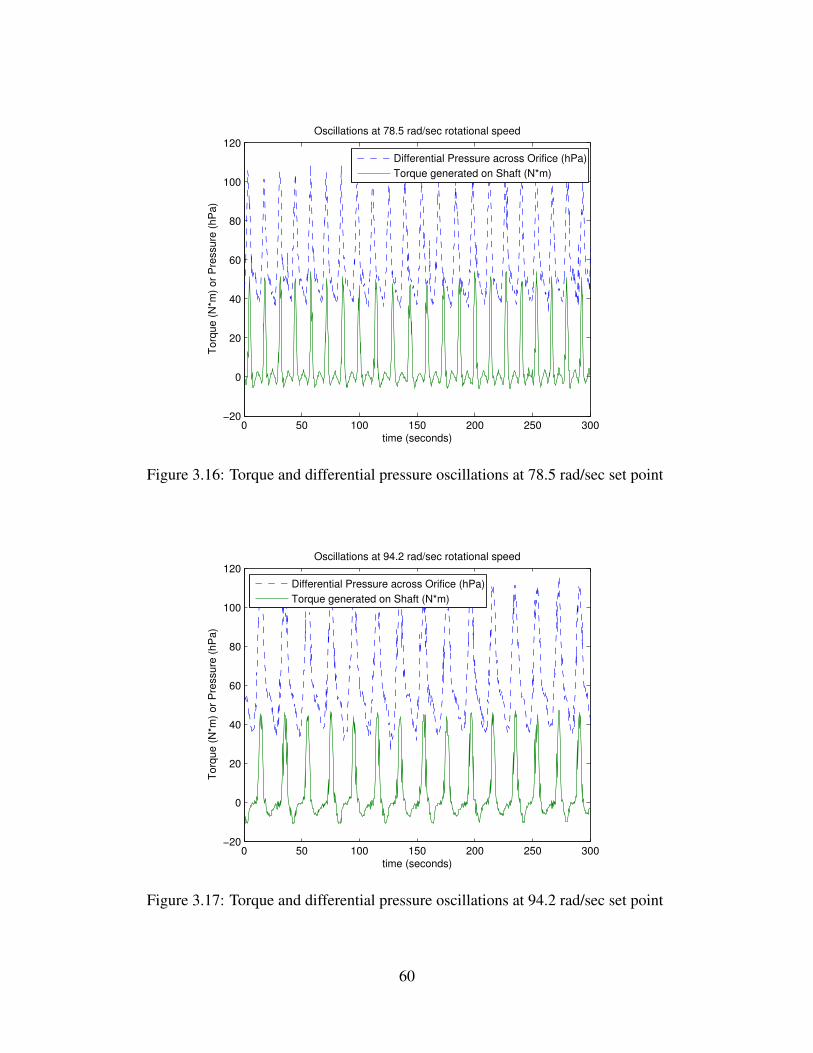
0 50 100 150 200 250 300!20
0
20
40
60
80
100
120
Torq
ue (
N*m
) o
r P
ress
ure
(hP
a)
time (seconds)
Oscillations at 78.5 rad/sec rotational speed
Differential Pressure across Orifice (hPa)
Torque generated on Shaft (N*m)
Figure 3.16: Torque and differential pressure oscillations at 78.5 rad/sec set point
0 50 100 150 200 250 300!20
0
20
40
60
80
100
120
Torq
ue (
N*m
) or
Pre
ssure
(hP
a)
time (seconds)
Oscillations at 94.2 rad/sec rotational speed
Differential Pressure across Orifice (hPa)
Torque generated on Shaft (N*m)
Figure 3.17: Torque and differential pressure oscillations at 94.2 rad/sec set point
60
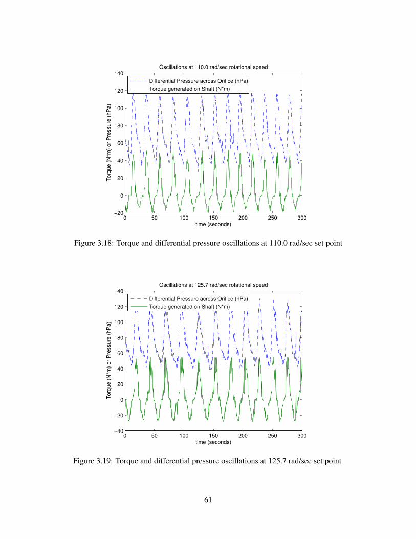
0 50 100 150 200 250 300!20
0
20
40
60
80
100
120
140
Torq
ue (
N*m
) o
r P
ress
ure
(hP
a)
time (seconds)
Oscillations at 110.0 rad/sec rotational speed
Differential Pressure across Orifice (hPa)
Torque generated on Shaft (N*m)
Figure 3.18: Torque and differential pressure oscillations at 110.0 rad/sec set point
0 50 100 150 200 250 300!40
!20
0
20
40
60
80
100
120
140
Torq
ue (
N*m
) or
Pre
ssure
(hP
a)
time (seconds)
Oscillations at 125.7 rad/sec rotational speed
Differential Pressure across Orifice (hPa)
Torque generated on Shaft (N*m)
Figure 3.19: Torque and differential pressure oscillations at 125.7 rad/sec set point
61
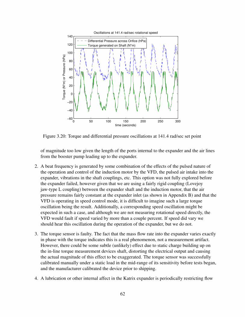
0 50 100 150 200 250 300!60
!40
!20
0
20
40
60
80
100
120
140
Torq
ue (
N*m
) or
Pre
ssure
(hP
a)
time (seconds)
Oscillations at 141.4 rad/sec rotational speed
Differential Pressure across Orifice (hPa)
Torque generated on Shaft (N*m)
Figure 3.20: Torque and differential pressure oscillations at 141.4 rad/sec set point
of magnitude too low given the length of the ports internal to the expander and the air linesfrom the booster pump leading up to the expander.
2. A beat frequency is generated by some combination of the effects of the pulsed nature ofthe operation and control of the induction motor by the VFD, the pulsed air intake into theexpander, vibrations in the shaft couplings, etc. This option was not fully explored beforethe expander failed, however given that we are using a fairly rigid coupling (Lovejoyjaw-type L coupling) between the expander shaft and the induction motor, that the airpressure remains fairly constant at the expander inlet (as shown in Appendix B) and that theVFD is operating in speed control mode, it is difficult to imagine such a large torqueoscillation being the result. Additionally, a corresponding speed oscillation might beexpected in such a case, and although we are not measuring rotational speed directly, theVFD would fault if speed varied by more than a couple percent. If speed did vary weshould hear this oscillation during the operation of the expander, but we do not.
3. The torque sensor is faulty. The fact that the mass flow rate into the expander varies exactlyin phase with the torque indicates this is a real phenomenon, not a measurement artifact.However, there could be some subtle (unlikely) effect due to static charge building up onthe in-line torque measurement devices shaft, distorting the electrical output and causingthe actual magnitude of this effect to be exaggerated. The torque sensor was successfullycalibrated manually under a static load in the mid-range of its sensitivity before tests began,and the manufacturer calibrated the device prior to shipping.
4. A lubrication or other internal affect in the Katrix expander is periodically restricting flow
62
rate into the expander. This type of problem would be a “breathing” effect as studiedextensively in engine design. The result of this effect would be both an oscillating torqueoutput and a mass flow oscillation, in agreement with measured results. Further explorationof the internal breathing of the Katrix expander and possibility of internal periodic blockageby lubricant (or something else) is recommended. All signs seem to indicate that flow isactually being restricted, unlikely to be caused by increased mechanical friction, but morelikely caused by an actual periodic restriction of the intake or exhaust pathways of the airthrough the expander.
Whatever the cause, the oscillating torque periodically saturates the sensor at its maximum valueas can be seen in figure 3.19 and figure 3.20. For this reason, these last two data runs, at thehighest rotational speeds tested, were not reported in the efficiency analysis.
3.5 Conclusions
It is worth noting that although I went to great pains to get good data, there are ways in whichthese efficiency results could overpredict (or underpredict) actual performance. Typically themass flow rate measurement is the most difficult to measure, but using multiple mass flow ratesensors in good agreement indicates this is not likely an issue. However, there were not redundantmeasurements for torque, temperature, nor downstream pressure in this test setup. If thedownstream temperature or pressure measurement was too high, upstream temperature too low, ortorque measured too high, these results would overpredict actual performance. There are severalfactors that lead me to believe the measured reading were indeed accurate. For instance theupstream piping was the right temperature to the touch, and frost formation on the expander outletindicated that thermocouple was certainly not reading too low. Pressure guages on the expanderinlet confirmed the sensor reading, but downstream pressure was harder to verify because theexpander outlet was vented to atmosphere. Lastly, the torque sensor was calibrated by themanufacturer, and then again under static load in our laboratory, but not under dynamic load.
It is clear from the results of testing that rotary lobe expanders exhibit great promise forsmall-scale efficient systems. Not only are the mechanisms simple and easy to manufacture, butan expansion ratio greater than 8:1 and demonstrated isentropic efficiency of 80-95% are best inclass. Detailed analysis of DCS-CHP systems (see Chapter 4) show that this combination ofefficiency and pressure ratio enables high overall solar-electric system efficiency. Furthermore,positive expansion devices can expand wet fluids, opening up the possibility of using water atsaturated conditions. Water is an excellent fluid to use for DCS-CHP systems because of itsbenign nature, ubiquity, and unsurpassed two-phase heat transfer properties. Additionally, theboiling point of water is well matched to the grades of heat used in residential and commercialestablishments. The next steps in development of an efficient rotary lobe expander for DCS-CHPapplications will be improving reliability, and design of lubricant-free bearings that work withcondensing steam.
63
Chapter 4
Simulation Framework for a DistributedConcentrating Solar Combined Heat andPower System
4.1 Introduction
A distributed concentrating solar combined heat and power system will use solar energy toprovide the heat input to a Rankine cycle to serve thermal and electrical loads. This system aimsto produce heat and electricity cost competitively with other renewable technologies, while beingsimple to manufacture. An efficient and low-cost heat engine is crucial to system efficacy and isthe main focus of research. Determining an appropriate working fluid and turbine design requiresmodeling the turbine performance as it interacts with all other system components. To accomplishthis, analytical models of expanders and certain aspects of solar thermal collectors have beencoded in Matlab software. These different simulations of Rankine cycle components providevaluable information, however analysis can only be done on individual components. A frameworkthat integrates each component of a Rankine cycle is important to predict overall cost andperformance.
Many components in a Rankine cycle system, when optimized, have adverse effects on other partsof the system. For example, high pressure ratios are good for maximizing cycle efficiency, buthigher pressure ratios often cause efficiency problems in the expander due to air leakage aroundthe rotor. Certain collectors operate at higher efficiencies with wet steam, but turbines often seeincreased wear with wet steam due to water droplets impinging on the blades. To facilitate thedesign and evaluation of a Distributed Concentrating Solar Combined Heat and Power(DCS-CHP) system, an advanced Rankine cycle simulation software that is able to modelinteractions between different component choices is useful. Because elements of a Rankine cycleoperate differently at varying pressures, temperatures, flow rates, vapor ratios, and weatherconditions, thermodynamic Rankine cycle analysis falls short of optimizing hardware-workingfluid interactions. In previous research, a model for performance of a small-scale radial inflow
64
turbine (Sunter et al. [35]) and Tesla turbines (Romanin et al. [30]) were analyzed, and Chapter 3shows the experimental results of a rotary lobe expander. This new tool can use these results tomodel interactions between the system and environment for the purpose of location-based designof appropriate technology. This tool uses an object-oriented framework, in Matlab software, thatcombines existing elements and allows addition of other elements – including heat exchangers,pumps, generators, turbines, solar collectors, and energy storage mechanisms. In this chapter, firstthe tool is described, and then results and analysis of a case study of the tool used for comparingappropriate expander and collector choices is demonstrated.
4.2 Program description
The program follows the Simulation-Environment-Agent framework. A Simulation containsseveral agents, called Systems, and several Environments. The Systems contain severalcomponents, which represent each element of a Rankine cycle (e.g. turbine, condenser, pump,generator, etc.). An Environment consists of weather data for a specific location. This data isuploaded from NREL’s National Solar Radiation Database. This program integrates the data intoa method of the Environment class. This method can be run (with an input of the imported data)to build Environment objects containing useful weather information including site name, sitelocation, typical insolation, typical temperatures, etc.
Components contain the necessary information to calculate the output state of a fluid based on theinput state. Currently all components are generic in that they do not contain any in-depth analysisof their operation - most operate simply with an isentropic efficiency. In the future, our advancedcomponent models will be coded into objects that can provide a more in-depth analysis ofcomponent operation.
Systems contain one of each component necessary for a Rankine cycle. When given constraintson the Rankine cycle, specifically the high temperature, high pressure, and low pressure of thesystem, the System is able to calculate the thermodynamic properties of the cycle (work output,heat output, energy input, solar-electric efficiency, etc.) by passing an input fluid state to thecomponent, which then returns an output fluid state (to be passed as input to the next component).
Fluid states are stored as properties of components. Each component has a StateIn and a StateOutproperty (for generators, PowerIn and PowerOut) that represent objects of the FluidState class.FluidState objects have the properties of Temperature, Pressure, Entropy, Enthalpy,InternalEnergy, Density, and Quality. These objects also have a FluidModel property that willaccommodate multiple fluids. Engineering Equation Solver or XSteam (by Excel Engineering)software calculates fluid properties. This allows systems to be analyzed with many differentworking fluids, including water.
Creating a Simulation object calls its GUI property. This brings up a graphical user interface(GUI) that displays a list of Environments and Systems contained in the Simulation. Environmentscan be added by running the getSitesFromSite method of Simulation with an input of the sitestructure, or by using the GUI. The site structure is is processed NREL TMY3 (TypicalMeteorological Year) data stored in the file SITESsaved.mat. This data can also be imported from
65

raw TMY data, but re-processing the raw data takes a significant amount of time compared toimporting preprocessed data.
System data can be added using the Add System button. Pressing the button brings up a GUIwith an image of a Rankine cycle. Next to each component of the Rankine cycle is a pop-up menuthat allows the user to select the type of component. The user can also select efficiencies andinput conditions to the cycle. Currently only default components exist, but additional componentswill be added as the code is developed. For example, the turbine pop-up menu currently onlyallows the user to select Turbine, which simply calculates output given a user-specified isentropicefficiency, but other expander types can be incorporated, which could allow configuration of therotor size, max speed, efficiency as a function of pressure ratio, etc. Once a system is configured,pushing the Save & Add System button constructs a System containing the components andreturns to the original GUI with the new System added.
Once Systems and Environments have both been added, any number of Systems and Environmentscan be selected from the respective lists. Clicking the Calculate button then analyzes eachpossible combination of System and Environment and returns the results.
66
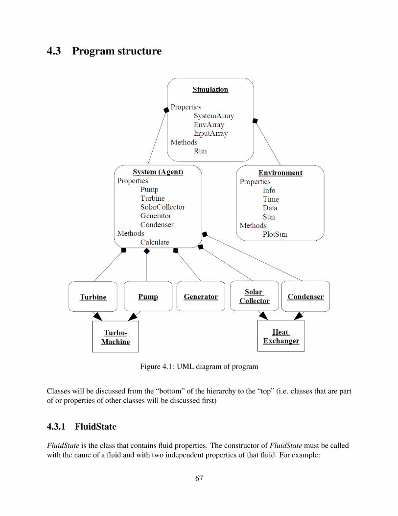
4.3 Program structure
Figure 4.1: UML diagram of program
Classes will be discussed from the “bottom” of the hierarchy to the “top” (i.e. classes that are partof or properties of other classes will be discussed first)
4.3.1 FluidState
FluidState is the class that contains fluid properties. The constructor of FluidState must be calledwith the name of a fluid and with two independent properties of that fluid. For example:
67
F = FluidState(‘water’,‘Pressure’,5,‘Temperature’,230)
A case statement then determines the two independent state properties, and enters the appropriateinputs into a fluid calculator. The constructor then populates the remaining properties ofFluidState (Temperature, Pressure, Entropy, Enthalpy, InternalEnergy, Density, and Quality) sothat all thermodynamic properties of the fluid are known. Instead of a property name and value,FluidState also accepts the strings ‘Saturated Liquid’ or ‘Saturated Vapor’, inwhich case the fluid calculator finds a state using one specified property at saturation conditions.FluidState also contains a property for the fluid model. All string inputs to FluidState are caseinsensitive.
4.3.2 Components
Components is not a class itself, but all mechanical elements of a Rankine cycle, includingturbines, pumps, generators, solar collectors, and condensers, are referred to as components.Some components inherit from a shared super class (e.g. Turbines and Pumps are bothTurboMachines, and Condensers and SolarCollectors are both HeatExchangers).
4.3.2.1 HeatExchangers
The HeatExchanger class contains the properties StateIn, StateOut, and Eta. It has a getHeatfunction that calculates the enthalpy difference between its StateOut and StateIn properties.
Condensers are HeatExchangers that remove heat from the Rankine cycle in the process ofcondensing the fluid from a vapor to a liquid. If no input is given to the constructor, all propertiesof Condenser are left blank. If one FluidState is given as an input, it is set to the Condenser’sStateIn property and Condenser’s calculate method is called with StateIn as an input.Condenser’s calculate method calculates StateOut by constructing a FluidState with inputs ofStateIn.Pressure and ‘Saturated Liquid’. In other words, the input to the condenser istypically partially or completely vapor; the output to the condenser is at the same pressure as theinput, but in a saturated liquid state.
SolarCollectors are HeatExchangers that transfer heat from the sun’s radiation into the workingfluid. SolarCollectors have a static method getDefaultEta that returns the default value for theefficiency of the collector. The constructor takes two inputs, stateIn and temperatureOut. If noinputs are specified, all properties of SolarCollector are left blank. If both inputs are specified,SolarCollector’s calculate method is called. If one or more than two inputs are specified, theconstructor returns an error. The calculate method takes three inputs aside from a collectorobject: stateIn, temperatureOut, and eta. If no eta is specified, a default eta is returned from thestatic method getDefaultEta. The calculate method than sets to StateOut a FluidState with thesame pressure as StateIn and with a temperature of temperatureOut (the specified hightemperature of the system).
68
4.3.2.2 TurboMachines
TurboMachine is an abstract class inherited by classes like Turbine and Pump. Similar toHeatExchanger, TurboMachine has three properties; StateIn, StateOut, and Eta. TurboMachinehas three methods, which calculate the volumetric ratio, pressure ratio, and work using the fluidproperties of StateIn and StateOut.
Turbines are TurboMachines that expand a fluid and produce work. The constructor of a Turbinetakes three inputs: a stateIn, pressureOut, and eta. If all three are specified, the calculate methodis called. If none are specified, the Turbine object is left blank. Turbine has a static method calledgetDefaultEta that returns a default value for the isentropic efficiency if none is specified. Thecalculate method takes in a Turbine object, a stateIn, pressureOut, and eta. StateIn is a FluidStatespecifying the inlet conditions. PressureOut is the low side pressure of the turbine. If no eta isspecified, the default eta is read from getDefaultEta. The calculate method then calculates theenthalpy of a constant entropy expansion (i.e. a FluidState with stateIn.Entropy and pressureOut),then multiplies the ideal enthalpy difference by the isentropic efficiency to find the actualenthalpy drop. This new enthalpy and pressureOut is used to determine Turbine.StateOut. Thecalculate function also outputs turbine work, which is calculated by subtracting the enthalpy ofStateOut from StateIn.
Pumps are TurboMachines that use work to compress a fluid. The constructor of a Pump worksexactly like that of a Turbine. The calculate method of a Pump functions like that of a Turbine,except that the work is calculated by subtracting the enthalpy of StateIn from StateOut.
4.3.2.3 Generators
Generators, unlike other components, have the properties of PowerIn, PowerOut (instead ofStateIn) and Eta. These properties are doubles as opposed to FluidStates. The PowerIn propertyis typically set to the work output of the Turbine, and the PowerOut is that work multiplied byEta. Like the other components, Generator has a static method called getDefaultEta. Theconstructor calls this method if no eta is entered. The calculate function for Generator takes in aGenerator object, powerin, and eta. The Generator.Eta property is set to eta (or to default if nonespecified) and the powerin value is set to Generator.PowerIn. The PowerOut property is thensimply the product of those two values. Calculate returns PowerOut.
4.3.3 System
The System class contains all the necessary information for one specific Rankine cycleconfiguration (i.e. one specific set of hardware). It has properties Pump, Turbine, Condenser,Generator, and SolarCollector; each being an object of its respective class. Currently, since onlydefault objects exist, these properties have the same names as the classes of objects that occupy
69
them. In the future as more types of each component are coded it is possible, for example, for theTurbine property to be a TeslaTurbine or a RotaryLobe. The constructor of System takes fiveinputs, one for each property. If a zero is specified, the constructor builds a default object of thattype. System has one method, calculate, which takes four inputs: System, Thigh, Phigh, and Plow.The last three inputs represent the constraints on the Rankine cycle, namely the input pressure andtemperature to the turbine and the exit pressure of the turbine.
To calculate all properties of the Rankine cycle, a FluidState is created with Thigh and Phigh asthe inputs. This fluid state and Plow are passed to System.Turbine’s calculate method, which thencreates the StateOut of Turbine and outputs the work of the turbine as turbineWork. TheCondenser then takes into its calculate function Turbine.StateOut, and produces its own StateOut(recall from basic thermodynamics that a Condenser is modeled as constant pressure heat removaluntil the fluid reaches saturated liquid). The output of Condenser.calculate (heatOut) is the heatoutput of the Rankine cycle. This heat can be used for domestic heating loads. NextPump.calculate is called with Condenser.StateOut and Phigh. This returns the fluid, nowcompletely liquid, to the high pressure of the system. The pump work is stored as pumpWork forlater calculating efficiencies. Finally SolarCollector.calculate is called with Pump.StateOut (highpressure liquid) and Thigh. SolarCollector.StateOut is calculated by raising the temperature of thefluid to the high temperature of the system. This value, the heat input to the solar collector, isstored as heatIn. Now the calculate method of Generator is called with turbineWork as an input,which then calculates and sets the Generator.PowerOut property and outputs generatorElec, theamount of electricity generated.
The heat and work inputs and outputs to the system are used to calculate the heat engineefficiency etaTherm, the solar to electric efficiency systemElecEta, the solar to heat efficiencysystemHeatEta, and the fraction of Carnot efficiency achieved fractionCarnotElec. The latterthree values are then set to the output of System.calculate.
4.3.4 Environment
Environment objects store the weather data processed from NREL’s TMY3 database. Nearly allEnvironments will be built using Simluation.getSitesFromSite, which is called through the GUI.Each of Environment’s properties; Info, Time, Data, and Sun, are structures that contain all thedata from the TMY database. Environment has one method, PlotTestSunData. When taking as aninput a day of the year (1 to 365), this function plots the insolation over the course of a day at thatEnvironment’s location for a typical year. This plot provides a visual representation of that site’sradiation as shown in figure 4.2.
4.3.5 Simulation
The Simulation class properties are an array of all the Systems, their names, and the inputs tothose Systems. Its methods include a constructor, which by default sets all properties to empty cellarrays, a Run function that calculates the performance of every possible combination of systems
70
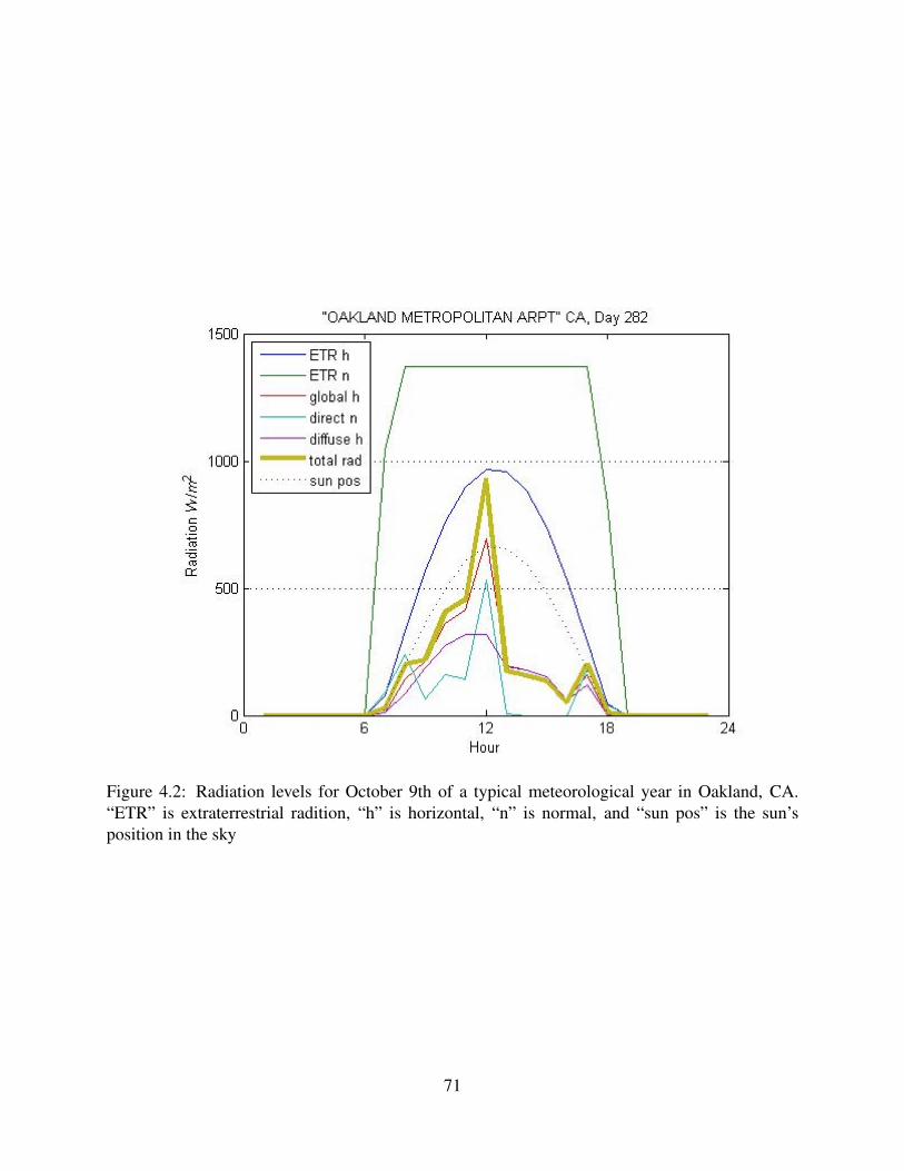
Figure 4.2: Radiation levels for October 9th of a typical meteorological year in Oakland, CA.“ETR” is extraterrestrial radition, “h” is horizontal, “n” is normal, and “sun pos” is the sun’sposition in the sky
71
and environments selected on the GUI, and a Plot function, which plots the simulation resultsshowing seasonal heat and electricity output for a single system at any number of selected sites.The plot function calls PlotUSLevels, a function to display seasonal and yearly data on latitudeand longitude axis.
4.3.5.1 Simulation GUI
The Gui function of the Simulation class provides an interface to select as many differentenvironment and system combinations as desired for simulation. Callback functions are used toprocess data, call the system GUI or plot the results GUI. The results GUI allows the user toselect yearly total heat or electricity output generated by the system and plot it in both seasonaland yearly form.
4.4 Operation of the simulation software
After navigating to the correct Matlab path, the software can be run as follows:
1. Start the Simulation at the command prompt by typing >> S = Simulation()
2. The Simulation GUI will pop up (figure 4.4), and the first step is to select Add System,which will bring up the System GUI (figure 4.3):
72
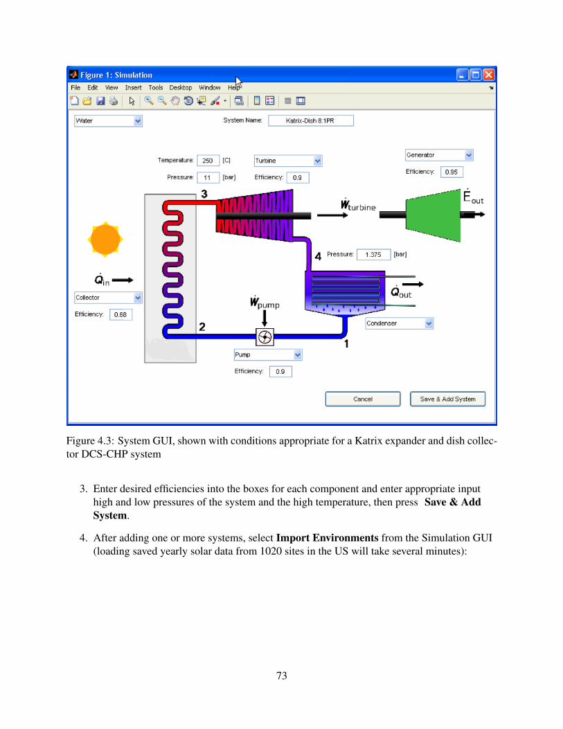
Figure 4.3: System GUI, shown with conditions appropriate for a Katrix expander and dish collec-tor DCS-CHP system
3. Enter desired efficiencies into the boxes for each component and enter appropriate inputhigh and low pressures of the system and the high temperature, then press Save & AddSystem.
4. After adding one or more systems, select Import Environments from the Simulation GUI(loading saved yearly solar data from 1020 sites in the US will take several minutes):
73
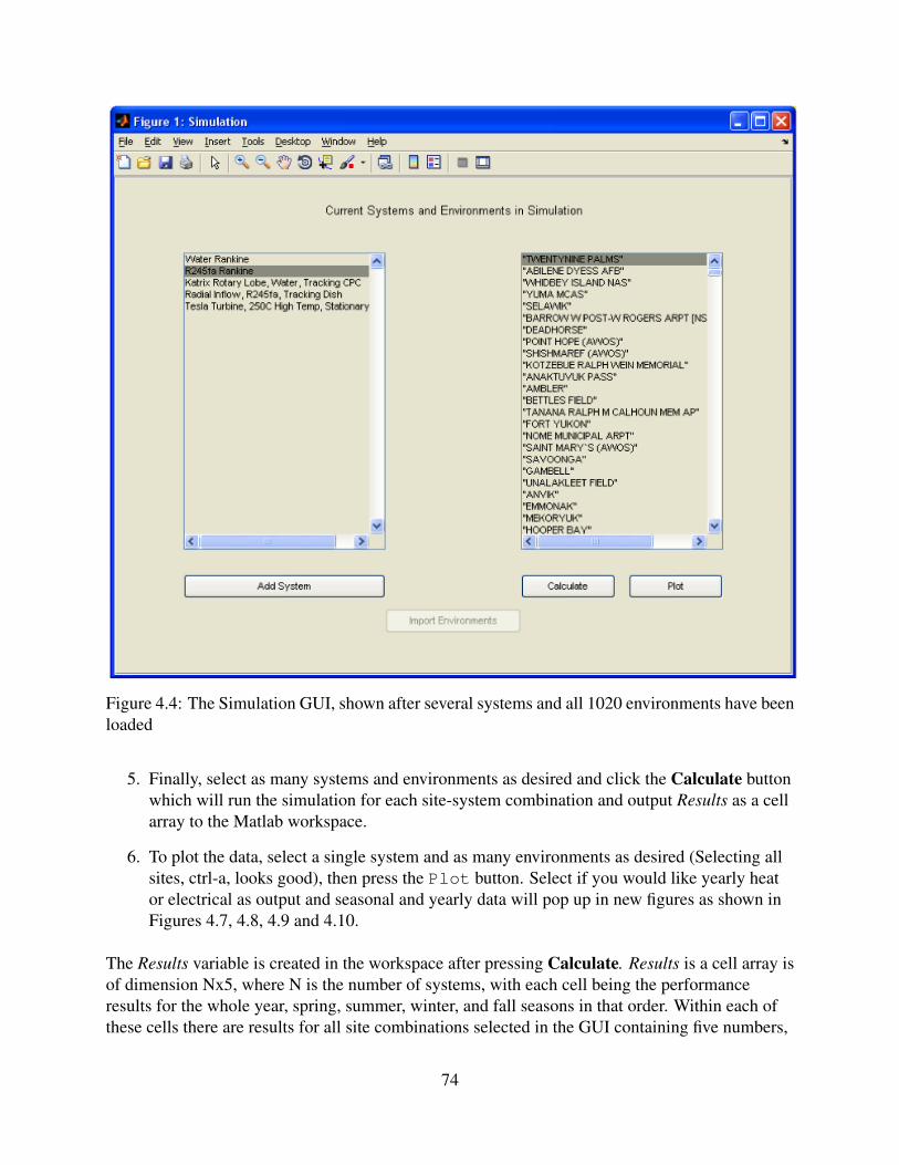
Figure 4.4: The Simulation GUI, shown after several systems and all 1020 environments have beenloaded
5. Finally, select as many systems and environments as desired and click the Calculate buttonwhich will run the simulation for each site-system combination and output Results as a cellarray to the Matlab workspace.
6. To plot the data, select a single system and as many environments as desired (Selecting allsites, ctrl-a, looks good), then press the Plot button. Select if you would like yearly heator electrical as output and seasonal and yearly data will pop up in new figures as shown inFigures 4.7, 4.8, 4.9 and 4.10.
The Results variable is created in the workspace after pressing Calculate. Results is a cell array isof dimension Nx5, where N is the number of systems, with each cell being the performanceresults for the whole year, spring, summer, winter, and fall seasons in that order. Within each ofthese cells there are results for all site combinations selected in the GUI containing five numbers,
74
corresponding to (1) solar-thermal efficiency, (2) solar-electric efficiency, (3) fraction of Carnotefficiency for electrical generation, (4) total yearly heat output at that site, and (5) total yearlyelectrical output at that site. The following is an example of the Matlab output as reported inTable 4.1:
>> Results{1}{1}ans =0.5833 0.0919 0.5267 969.5886 152.7057
4.5 Case study of an appropriate DCS-CHP system
There is demand today for Distributed Concentrating Solar Combined Heat and Power(DCS-CHP), as demonstrated by the strong growth in photovoltaics and recent growth insolar-thermal heating, but DCS-CHP technology does not exist in the marketplace today to fillthat niche. The two technical challenges that have been prohibitive towards the development of aDCS-CHP system are the cost of the solar collector and the efficiency of a small-scale turbine.Continuing innovation in these areas combined with advanced system analysis and design nowmake such a system possible. One such expander and collector combination is described andevaluated below.
4.5.1 The Orbital Concentrator
One of the fundamental technologies we explore is a new type of solar collector optimallydesigned for DCS-CHP applications, referred to as the Orbital Concentrator, conceived with thefounders of Raw Solar (RawSolar [27]). This technology combines high concentration opticswith a compact and static plumbing system, enabling excellent efficiency at working temperatureshigh enough for efficient steam Rankine cycle performance, while reducing capital andoperational costs. This new Orbital Concentrator is a fundamentally different form of solarconcentrator, a hybrid balancing the pros and cons of traditional dish and power-tower systems.There is one receiver per reflector, like a dish, but the receiver is fixed in place while the reflectororbits around it following the sun. Specifically, the reflector rotates around a vertical axis passingthrough the receiver to track the azimuth angle of the sun, and simultaneously tilts up and downand translates in and out to track the zenith angle of the sun while maintaining a fixed focal lengthbetween the reflector and the receiver so as to keep a sharp focus on the receiver (Figure 4.5).
Dishes have been well explored by many organizations, including the US Department of Energy.Notable systems include LaJet, SES, and Zenith. Like traditional dishes, Orbital Concentratorshave the advantage of achieving very high concentration ratios, suffer near-zero cosine losses, andare robust to tracking and slope error because of their relatively short focal length. Dishes,however, are poorly suited for heating a high temperature working fluid to power a remote heatengine, as the fluid plumbing must be routed circuitously through the dish structure and mustinclude articulate joints. These joints pose significant costs as they must handle continuous
75
(a)
(b)
Figure 4.5: Orbital Concentrator (a) tracking motion and (b) comparison of summer day poweroutput versus dish
76
movement while transporting hot and potentially high pressure fluids, and are known to be aprimary failure point of many dish and trough systems, including the SEGS plants. Thesecomplications have led most dish implementations to use self-contained systems (typicallyStirling engines or CPV modules) for electricity production, avoiding the need for these joints butrestricting CHP options.
Having a remote heat engine has many advantages over a focal-mounted engine (e.g.dish-Stirling) by decoupling the two components. Vibrational decoupling decreases fatigue on thestructure, yielding longer life and lower cost, and increases tracking performance by reducingnoise to the sensors. Decoupling of scale allows several smaller collectors to power one largerengine. Smaller collectors are more cost effective because they have significantly lower windloads, can use off-the-shelf actuators, and are more ground-supported. Larger engines are lowercost per watt, more efficient, and have lower operational costs per kWh produced. There is alsono need to suspend the weight of the entire thermal-electric system up in the air, further reducingstructural costs.
Power towers have also been well explored, notably by BrightSource, Solar Two, and PS10. Justas in power-tower systems, the receiver and plumbing in the Orbital Concentrator are fixed,eliminating the complications of movable plumbing joints. Power-towers, however, have severaldisadvantages that are avoided by the Orbital Concentrator. They must be of very large scale inorder to work efficiently, restricting CHP and distributed applications because they typically mustbe sited very far from energy loads. The heliostats suffer from moderate cosine losses, reducingmaterial efficiency. The distance from reflector to receiver target is very large, reducingconcentration factors and robustness to tracking and slope error. Towers are typically over 100meters tall with the thermal-electric system located at the top, adding significant complexity andcost.
This novel Orbital Concentrator is highly conducive for low-cost mass production, rapid scale up,and ease of deployment by leveraging commodity materials, the existing manufacturing base, andoff-the-shelf components. One of the historical challenges of building two-axis concentrators isthe manufacture of the compound reflector surface. The Orbital Concentrator uses the techniqueof arraying single-axis reflector slats to form a hybrid Fresnel reflector surface, suitable for anynumber of reflector laminates such as flexed mirrored glass, metal sheeting (such as Miro byAlanod), or Mylar films (such as ReflecTech). It is unclear which of these reflector options isideal, but the Orbital Concentrator will work with all of the above and testing could be done toselect an ideal candidate for mass-production. Using flat reflector strips allows the compoundstructure to be assembled out of easily mass-produced reflector modules, sourced by existingmanufacturing entities. The compound surface has a concentration ratio in the Fresnel directionon the order of the number of slats, whereas the flexed axis can achieve much higherconcentration because of the continuous curvature. This combination is conducive to a short andwide configuration of a few long horizontal strips, and thus the final dimension can be matchedfor easy stacking and packing into standard shipping containers for efficient transportation to thedeployment site.
There are of course trade-offs with the Orbital Concentrator compared to power-tower and dishsystems, but they have been carefully balanced in consideration of the over-all system. For
77
example, the Orbital Concentrator cannot achieve concentration factors as high as high-fidelitydishes because it operates slightly off-axis for a portion of every day and has a hybrid Fresnelsurface. Fortunately, higher concentration is only necessary for significantly higher temperatures,which are not the goal of this project because they increase costs significantly. Based onfirst-order engineering calculations, the Orbital Concentrator will be able to achieve 500xconcentration, which is more than adequate to generate steam at over 75% efficiency and of thepressure and temperature needed to operate the Katrix expander effectively. Orbital Concentratorsalso suffer from slight cosine losses compared to dishes, but engineering analysis shown in Figure4.5 indicates this loss is on the order of 2%. A worst-case comparison of the daily power profilesof a dish and Orbital Concentrator exhibits the highest instantaneous loss of about 6% when thesun is highest in the sky, but an average loss of about 2% over the course of the day. The finaltrade-off is that a smaller system has limited thermal-electric conversion efficiency compared topower-towers, but this is lost in favor of modular, distributed, CHP generation.
4.5.2 The Rankine cycle powering a Katrix rotary lobe expander
The second enabling technology for this DCS-CHP system is an efficient small-scale rotary lobeexpander. As Aoun concludes in his thesis on the subject of residential solar CHP, volumetricexpansion devices like Wankels, vane expanders, and screws/scrolls are the most promising fordistributed applications (Aoun [1]). The problem with small expanders in general is that the powergenerated is proportional to the displaced volume, however many losses are proportional to thesurface area (e.g. friction on moving seals/rings in positive displacement machines), so shrinkingthe expander size decreases the overall efficiency because volume is a function of the cube of thecharacteristic dimension, whereas surface area is a function of the square of that dimension. Thiseffect is what makes Tesla turbines so interesting in small-scale in that they turn this relationshiparound since power is generated by viscous forces, dragging on the rotor, which actually increases(inversely to volumetric flow rate) as the size of the device is scaled down. Much work still needsto be done in improving Tesla turbines however, and it is unclear whether they will reachefficiencies in the useful realm for this application (Romanin et al. [30]), although some work hasindicated it is possible they already have (Saitoh et al. [31]) . Aerodynamic turbines, even thoseused in the smallest scale commercial applications, radial inflow turbines, are also incompatiblewith the high pressure ratios and low power outputs needed for DCS-CHP (Sunter et al. [35]) .
That leaves screw, scroll, piston, vane, and rotary lobe expanders (e.g. Wankel). Of those, screwand scroll expanders exhibit modest performance in small-scale (Aoun [1]), and pistons showgood performance, but at the cost of more complex valves and more moving parts than rotary lobeexpanders. Vane expanders have not been explored thoroughly in this research but may sufferfrom lower efficiencies than other volumetric devices at high pressure ratios (Aoun [1]). For thosereasons the rotary lobe expander appears nearly ideal for DCS-CHP if good pressure ratios andperformance can be achieved with the desired working fluid.
The current generation Katrix expander was experimentally verified to provide an 8:1 pressureexpansion ratio at greater than 80% isentropic efficiency, as reported in Chapter 3. Thistechnology, originally developed for waste heat applications with funding from the Australian
78
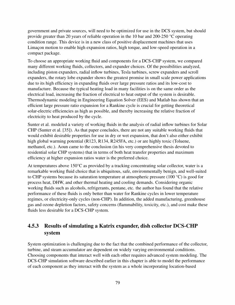
government and private sources, will need to be optimized for use in the DCS system, but shouldprovide greater than 20 years of reliable operation in the 10 bar and 200-250 °C operatingcondition range. This device is in a new class of positive displacement machines that usesLimaçon motion to enable high expansion ratios, high torque, and low-speed operation in acompact package.
To choose an appropriate working fluid and components for a DCS-CHP system, we comparedmany different working fluids, collectors, and expander choices. Of the possibilities analyzed,including piston expanders, radial inflow turbines, Tesla turbines, screw expanders and scrollexpanders, the rotary lobe expander shows the greatest promise in small scale power applicationsdue to its high efficiency in expanding fluids over large pressure ratios and its low-cost tomanufacture. Because the typical heating load in many facilities is on the same order as theelectrical load, increasing the fraction of electrical to heat output of the system is desirable.Thermodynamic modeling in Engineering Equation Solver (EES) and Matlab has shown that anefficient large pressure ratio expansion for a Rankine cycle is crucial for getting theoreticalsolar-electric efficiencies as high as possible, and thereby increasing the relative fraction ofelectricity to heat produced by the cycle.
Sunter et al. modeled a variety of working fluids in the analysis of radial inflow turbines for SolarCHP (Sunter et al. [35]). As that paper concludes, there are not any suitable working fluids thatwould exhibit desirable properties for use in dry or wet expansion, that don’t also either exhibithigh global warming potential (R123, R134, R245FA, etc.) or are highly toxic (Toluene,methanol, etc.). Aoun came to the conclusion (in his very comprehensive thesis devoted toresidential solar CHP systems) that in terms of both heat transfer properties and maximumefficiency at higher expansion ratios water is the preferred choice.
At temperatures above 150°C as provided by a tracking concentrating solar collector, water is aremarkable working fluid choice that is ubiquitous, safe, environmentally benign, and well-suitedto CHP systems because its saturation temperature at atmospheric pressure (100 °C) is good forprocess heat, DHW, and other thermal heating and cooling demands. Considering organicworking fluids such as alcohols, refrigerants, pentane, etc. the author has found that the relativeperformance of these fluids is only better than water for Rankine cycles in lower temperatureregimes, or electricity-only cycles (non-CHP). In addition, the added manufacturing, greenhousegas and ozone depletion factors, safety concerns (flammability, toxicity, etc.), and cost make thesefluids less desirable for a DCS-CHP system.
4.5.3 Results of simulating a Katrix expander, dish collector DCS-CHPsystem
System optimization is challenging due to the fact that the combined performance of the collector,turbine, and steam accumulator are dependent on widely varying environmental conditions.Choosing components that interact well with each other requires advanced system modeling. TheDCS-CHP simulation software described earlier in this chapter is able to model the performanceof each component as they interact with the system as a whole incorporating location-based
79
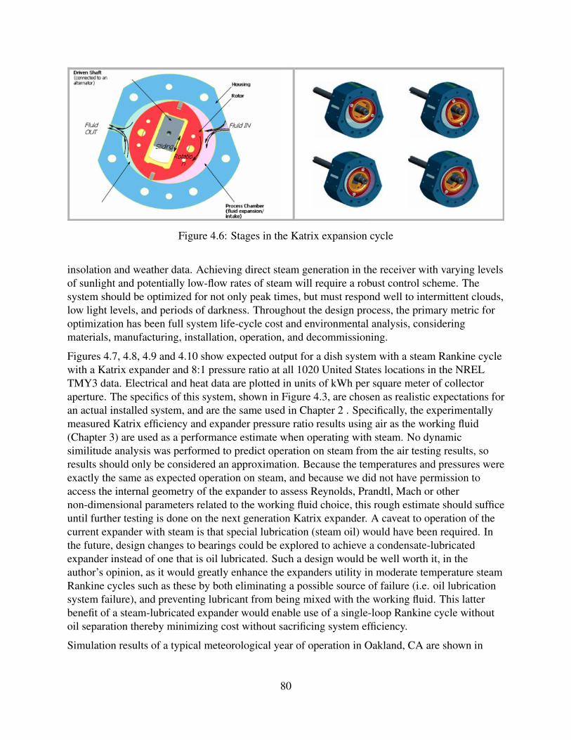
Figure 4.6: Stages in the Katrix expansion cycle
insolation and weather data. Achieving direct steam generation in the receiver with varying levelsof sunlight and potentially low-flow rates of steam will require a robust control scheme. Thesystem should be optimized for not only peak times, but must respond well to intermittent clouds,low light levels, and periods of darkness. Throughout the design process, the primary metric foroptimization has been full system life-cycle cost and environmental analysis, consideringmaterials, manufacturing, installation, operation, and decommissioning.
Figures 4.7, 4.8, 4.9 and 4.10 show expected output for a dish system with a steam Rankine cyclewith a Katrix expander and 8:1 pressure ratio at all 1020 United States locations in the NRELTMY3 data. Electrical and heat data are plotted in units of kWh per square meter of collectoraperture. The specifics of this system, shown in Figure 4.3, are chosen as realistic expectations foran actual installed system, and are the same used in Chapter 2 . Specifically, the experimentallymeasured Katrix efficiency and expander pressure ratio results using air as the working fluid(Chapter 3) are used as a performance estimate when operating with steam. No dynamicsimilitude analysis was performed to predict operation on steam from the air testing results, soresults should only be considered an approximation. Because the temperatures and pressures wereexactly the same as expected operation on steam, and because we did not have permission toaccess the internal geometry of the expander to assess Reynolds, Prandtl, Mach or othernon-dimensional parameters related to the working fluid choice, this rough estimate should sufficeuntil further testing is done on the next generation Katrix expander. A caveat to operation of thecurrent expander with steam is that special lubrication (steam oil) would have been required. Inthe future, design changes to bearings could be explored to achieve a condensate-lubricatedexpander instead of one that is oil lubricated. Such a design would be well worth it, in theauthor’s opinion, as it would greatly enhance the expanders utility in moderate temperature steamRankine cycles such as these by both eliminating a possible source of failure (i.e. oil lubricationsystem failure), and preventing lubricant from being mixed with the working fluid. This latterbenefit of a steam-lubricated expander would enable use of a single-loop Rankine cycle withoutoil separation thereby minimizing cost without sacrificing system efficiency.
Simulation results of a typical meteorological year of operation in Oakland, CA are shown in
80

200
400
600
800
1000
1200
1400
1600
Figure 4.7: Katrix-Dish system yearly heat output (scale is kWh thermal per m^2 of collectoraperture)
81
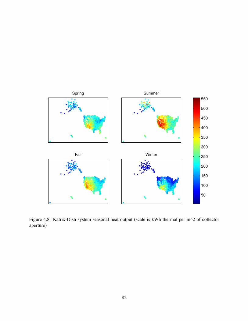
Spring Summer
Fall Winter
50
100
150
200
250
300
350
400
450
500
550
Figure 4.8: Katrix-Dish system seasonal heat output (scale is kWh thermal per m^2 of collectoraperture)
82
50
100
150
200
250
Figure 4.9: Katrix-Dish system yearly electrical output (scale is kWh electric per m^2 of collectoraperture)
83
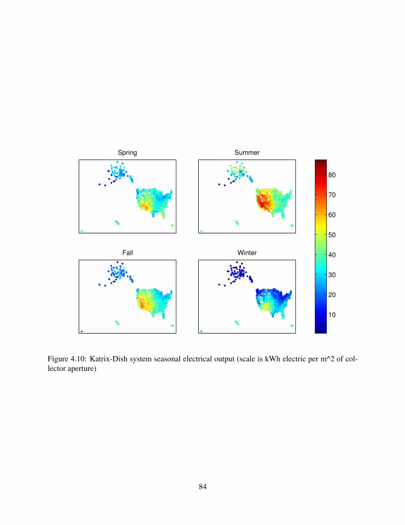
Spring Summer
Fall Winter
10
20
30
40
50
60
70
80
Figure 4.10: Katrix-Dish system seasonal electrical output (scale is kWh electric per m^2 of col-lector aperture)
84
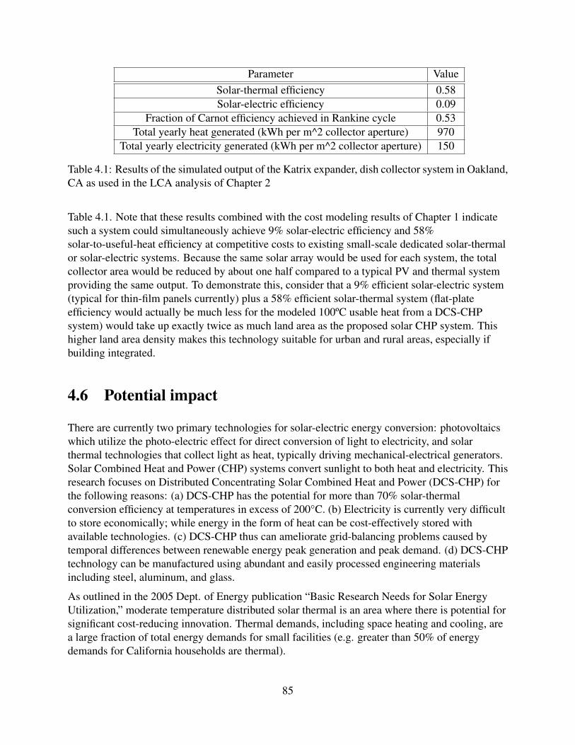
Parameter ValueSolar-thermal efficiency 0.58Solar-electric efficiency 0.09
Fraction of Carnot efficiency achieved in Rankine cycle 0.53Total yearly heat generated (kWh per m^2 collector aperture) 970
Total yearly electricity generated (kWh per m^2 collector aperture) 150
Table 4.1: Results of the simulated output of the Katrix expander, dish collector system in Oakland,CA as used in the LCA analysis of Chapter 2
Table 4.1. Note that these results combined with the cost modeling results of Chapter 1 indicatesuch a system could simultaneously achieve 9% solar-electric efficiency and 58%solar-to-useful-heat efficiency at competitive costs to existing small-scale dedicated solar-thermalor solar-electric systems. Because the same solar array would be used for each system, the totalcollector area would be reduced by about one half compared to a typical PV and thermal systemproviding the same output. To demonstrate this, consider that a 9% efficient solar-electric system(typical for thin-film panels currently) plus a 58% efficient solar-thermal system (flat-plateefficiency would actually be much less for the modeled 100ºC usable heat from a DCS-CHPsystem) would take up exactly twice as much land area as the proposed solar CHP system. Thishigher land area density makes this technology suitable for urban and rural areas, especially ifbuilding integrated.
4.6 Potential impact
There are currently two primary technologies for solar-electric energy conversion: photovoltaicswhich utilize the photo-electric effect for direct conversion of light to electricity, and solarthermal technologies that collect light as heat, typically driving mechanical-electrical generators.Solar Combined Heat and Power (CHP) systems convert sunlight to both heat and electricity. Thisresearch focuses on Distributed Concentrating Solar Combined Heat and Power (DCS-CHP) forthe following reasons: (a) DCS-CHP has the potential for more than 70% solar-thermalconversion efficiency at temperatures in excess of 200°C. (b) Electricity is currently very difficultto store economically; while energy in the form of heat can be cost-effectively stored withavailable technologies. (c) DCS-CHP thus can ameliorate grid-balancing problems caused bytemporal differences between renewable energy peak generation and peak demand. (d) DCS-CHPtechnology can be manufactured using abundant and easily processed engineering materialsincluding steel, aluminum, and glass.
As outlined in the 2005 Dept. of Energy publication “Basic Research Needs for Solar EnergyUtilization,” moderate temperature distributed solar thermal is an area where there is potential forsignificant cost-reducing innovation. Thermal demands, including space heating and cooling, area large fraction of total energy demands for small facilities (e.g. greater than 50% of energydemands for California households are thermal).
85
The value proposition for Distributed Generation (DG) compared to centralized generation favorsDG for several reasons: (a) The price for DG compares to electricity and natural gas (or fuel oil)at retail cost, not wholesale cost, as consumers will be producing electricity and displacing naturalgas (or fuel oil) at the site of end-use. The retail cost of electricity is approximately 100% higherthan wholesale, giving DG this considerable advantage. (b) DCS-CHP is capable of efficientlyoffsetting domestic demands for heating and cooling, unlike utility scale systems, which are notlocated in close enough proximity to end-users to take much advantage of the rejected waste heatfrom power generation. (c) Electrical transmission concerns are alleviated because power is beinggenerated at or near the point of use, where existing transmission infrastructure often alreadyexists.
The combined advantages of distributed generation and solar-thermal CHP have the potential tomake this a transformative technology. Solar PV, wind, geothermal, and hydropower are currentlythe leading technologies for distributed renewable power generation; however several barriersprevent these technologies from being ubiquitous. Local environmental resources limit wind,geothermal, and hydropower; while solar energy is nearly universally available, although invarying amounts. Photovoltaics are functional in a much wider range of environments, howeverthe scarcity of required materials, lower efficiencies, and the complexity of manufacturing makethem costly and impractical for rapid and universal adoption. DCS-CHP has the advantage ofusing solar energy while overcoming the manufacturing difficulties of photovoltaics, giving it apotential for deep market penetration of renewable distributed energy generation. Additionally,the ability to create both heat and power, adjustable on demand, allows the proposed system tooffset imports from foreign fossil fuel sources (e.g. natural gas and fuel oil), and also greatlyimpact regional GHG emissions from electricity production (e.g. coal power plants).
According to the Energy Information Administration’s 2007 Annual Energy Review, fossil fuels(including petroleum) in the commercial, industrial, and residential sectors account for more thanhalf of the total energy used in the United States, with transportation accounting for less than 30%of this. Because DCS-CHP targets both heat and power generation in buildings, it has the abilityto reduce fossil fuel usage dramatically.
A Life Cycle Assessment of DCS-CHP has been conducted in order to select low-cost,non-polluting and widely available materials. The calculated greenhouse gases emitted fromelectricity produced by DCS-CHP is 5 to 10 times lower than that same unit of electricitytypically consumed in the United States, and the ease of recycling the DCS-CHP system furtherreduces GHG emissions at the end of the product’s life. This result lies in the same emissionrange as other renewable energy technologies in solar thermal and PV, and ensures that as thedemand in DCS-CHP increases prices will not fluctuate due to material scarcity or an increasedcost of carbon emissions. The levelized cost of energy generated by the DCS-CHP system over itslifetime is estimated to be $0.25/kWh electric, and $0.03/kWh of a 100ºC heat source, or $3.20/Welectric and $0.40/W thermal based on installed capital cost per peak power output. The LCA ofthe system affirms that small scale solar combined heat and power systems can directly competewith other renewable energy systems and have comparable environmental impacts to PV systems.
The proposed DCS-CHP system, in the 1-10 kW peak electric range, will be appropriate for smallresidential communities or single households with reasonable land area. Commercial and
86

industrial applications could be served by a solar orchard, consisting of many solar dishes arrayedon rooftops, above parking lots, or in open fields, hillsides, etc. For congested areas, this districtsystem can supply heat and power to local residences or businesses. Although it may seem thatthe decreased efficiency of solar-electric conversion, for a distributed system (~10%) as comparedto a centralized CSP plant (>20%), would decrease efficiency of the energy generation sector as awhole, this is not the case. First, the heat generated by this system, if put to use displacing fossilfuels would more than make up for the decreased solar-electric efficiency, especially whencomparing relative GHG intensities. Secondly, distributed generation effectively bypasses manyof the hurdles found in siting and permitting other renewable energy generation technologies ortransmission lines, which limit the speed at which fossil fuel generation can be replaced. Also, thenumber of green jobs created by a DG technology is greater than that of a centralized technologydue to the increased labor force needed to install, maintain, and operate many small systems, ascompared to a typical large central generation plant. And lastly, although oft overlooked,distributed energy generation technology promotes democracy in energy choices by putting thegeneration equipment in the hands of the consumer instead of the corporations that typicallycontrol centralized energy generation.
87

Bibliography
[1] Aoun, B. (2009, May). Micro combined heat and power operating on renewable energy forresidential building. Ph. D. thesis, Ecole Doctorale 432 Sciences des Métiers de l’Ingénieur.
[2] Appropedia (2011, April). Levelised cost of electricity literature review.http://www.appropedia.org/.
[3] Blevins, R. (2003). Applied fluid dynamics handbook. Krieger Pub.
[4] Casten, T. R. and R. U. Ayres (2007). Energy myth eight – worldwide power systems areeconomically and environmentally optimal. In Energy and American Society – ThirteenMyths. Springer Netherlands.
[5] Çengel, Y. A. and M. A. Boles (2006). Thermodynamics: an engineering approach (5 ed.).McGraw-Hill Higher Education.
[6] El-Dessouky, H. T., H. M. Ettouney, and F. Mandani (2000). Performance of parallel feedmultiple effect evaporation system for seawater desalination. Applied ThermalEngineering 20(17), 1679 – 1706.
[7] Gleick, P. H. (1994). Water and energy. Annual Review of Energy and theEnvironment 19(1), 267–299.
[8] Hansen, J., M. Sato, P. Kharecha, D. Beerling, R. Berner, V. Masson-Delmotte, M. Pagani,M. Raymo, D. Royer, and J. Zachos (2008). Target atmospheric CO2: Where should humanityaim? Open Atmospheric Science Journal 2, 217–231.
[9] Hendrickson, C., A. Horvath, S. Joshi, M. Klausner, L. Lave, and F. McMichael (1997, May).Comparing two life cycle assessment approaches: a process model vs. economicinput-output-based assessment. In Electronics and the Environment, 1997. ISEE-1997.,Proceedings of the 1997 IEEE International Symposium on, pp. 176–181.
[10] IEEE (2009). IEEE application guide for IEEE std 1547, IEEE standard for interconnectingdistributed resources with electric power systems. IEEE Std 1547.2-2008, 1 –207.
[11] Kalogirou, S. (1997). Survey of solar desalination systems and system selection.Energy 22(1), 69 – 81.
88
[12] Kalogirou, S. A. (2004). Solar thermal collectors and applications. Progress in Energy andCombustion Science 30(3), 231 – 295.
[13] Kalogirou, S. A. (2005). Seawater desalination using renewable energy sources. Progress inEnergy and Combustion Science 31(3), 242 – 281.
[14] Lenzen, M. (2008). Life cycle energy and greenhouse gas emissions of nuclear energy: Areview. Energy Conversion and Management 49(8), 2178 – 2199.
[15] Lewis, N. S., G. Crabtree, A. J. Nozik, M. R. Wasielewski, P. Alivisatos, H. Kung, J. Tsao,E. Chandler, W. Walukiewicz, M. Spitler, R. Ellingson, R. Overend, J. Mazer, M. Gress,J. Horwitz, C. Ashton, B. Herndon, L. Shapard, and R. M. Nault (2005, April). Basic researchneeds for solar energy utilization. Technical report, US DOE - Office of Basic EnergySciences.
[16] Mahjouri, F. (2004). Vacuum tube liquid-vapor (heat-pipe) collectors. Proceedings of theASES Solar 2004 Conference.
[17] Mathworks (2011, March). http://www.mathworks.com/help/techdoc/ref/std.html.
[18] Mills, D. (2004). Advances in solar thermal electricity technology. Solar Energy 76(1-3), 19– 31. Solar World Congress 2001.
[19] Montgomery, Z. (2009, December). Environmental impact study: CSP vs. CdTe thin filmphotovoltaics. Master’s thesis, Duke University.
[20] Müller-Steinhagen, H. (2004). Durability, reliability and performance of a solar collector.Technical report, University of Stuttgart.
[21] Norwood, Z., N. Kamphuis, and D. Soltman (2006, December). Distributedsolar-thermal/electric generation. Technical report, University of California at Berkeley, CA(US).
[22] Norwood, Z., T. Lipman, M. Stadler, and C. Marnay (2010). Assessment of combined heatand power "premium power" applications in California. International Journal of DistributedEnergy Resources 6(2), 131–147.
[23] Norwood, Z., S. Pepe, V. Romanin, and D. Kammen (2010). Performance-cost analysis ofsolar combined heat and power systems. ASME Conference Proceedings 2010(43956), 27–34.
[24] Pehnt, M. (2006). Dynamic life cycle assessment (LCA) of renewable energy technologies.Renewable Energy 31(1), 55 – 71.
[25] PG&E (2010, December). Pacific gas and electric rule no. 21: Generating facilityinterconnections.
[26] Price, H., E. Lupfert, D. Kearney, E. Zarza, G. Cohen, R. Gee, and R. Mahoney (2002).Advances in parabolic trough solar power technology. Journal of Solar EnergyEngineering 124(2), 109–125.
89
[27] RawSolar (2009, June). http://www.raw-solar.com/.
[28] Reich-Weiser, C., S. Horne, and D. A. Dornfeld (2008). Environmental metrics for solarenergy. Technical report, University of California at Berkeley, Laboratory for Manufacturingand Sustainability.
[29] REN21 (2009). Renewables global status report: 2009 update. Technical report, RenewableEnergy Policy Network for the 21st Century.
[30] Romanin, V., V. P. Carey, and Z. Norwood (2010). Strategies for performance enhancementof Tesla turbines for combined heat and power applications. ASME ConferenceProceedings 2010(43956), 57–64.
[31] Saitoh, T., N. Yamada, and S.-i. Wakashima (2007). Solar Rankine cycle system using scrollexpander. Journal of Environment and Engineering 2(4), 708–719.
[32] Spencer, L. (1989a, January). A comprehensive review of small solar-powered heat enginespart II: Research since 1950-conventional engines up to 100kW. Solar Energy 43(4), 197–210.
[33] Spencer, L. (1989b, January). A comprehensive review of small solar-powered heat engines.part III: Research since 1950-unconventional engines up to 100 kW. Solar Energy 43(4),211–225.
[34] Stoppato, A. (2008). Life cycle assessment of photovoltaic electricity generation.Energy 33(2), 224 – 232. 19th International Conference on Efficiency, Cost, Optimization,Simulation and Environmental Impactof Energy Systems - ECOS 2006.
[35] Sunter, D. A., V. P. Carey, and Z. Norwood (2010). Radial inflow turbine assessment forsmall-scale concentrated solar Rankine combined heat and power technology. ASMEConference Proceedings 2010(43956), 45–56.
[36] Swamy, M. (2005). Passive techniques for reducing input current harmonics. Technicalreport, Yaskawa Electric America, Inc.
[37] Thomas, K. E. (1997, April). Overview of village scale, renewable energy powereddesalination. Technical Report NREL/TP–440-22083, National Renewable Energy Lab.,Golden, CO (United States).
[38] UNESCO (2010, December). Valuing water. http://www.unesco.org/.
[39] USDOE. Concentrating solar power commercial application study: Reducing waterconsumption of concentrating solar power electricity generation. Technical report, Report toCongress.
[40] Wade, N. M. (1999). Energy and cost allocation in dual-purpose power and desalinationplants. Desalination 123(2-3), 115 – 125. Selected papers presented at The WSTA Fourth GulfWater Conference.
90

[41] Weisman, A. (2008). Gaviotas: a village to reinvent the world. White River Junction, VT:Chelsea Green Pub. Co.
[42] Weiss, W., I. Bergmann, and R. Steizer (2009, May). Solar heat worldwide: Markets andcontribution to the energy supply 2007. Technical report, International Energy Agency SolarHeating and Cooling Programme.
[43] WHO and UNICEF (2010). Progress on sanitation and drinking-water: 2010 update.
[44] Wiser, R., G. Barbose, and C. Peterman (2009, February). Tracking the sun: The installedcost of photovoltaics in the U.S. from 1998-2007. Technical Report LBNL-1516E, ErnestOrlando Lawrence Berkeley National Laboratory, Berkeley, CA (US).
91

Chapter 5
Appendix A: Katrix Testing Equipment andData
92
5.1 Test equipment
This is a list of the main test equipment, including sensors’ make and model used in testing theKatrix expander:
• Upstream pressure transducer: Omega PX26-250GV
• Downstream pressure transducer: Omega PX181-300G5V
• Differential (Orifice) pressure transducer: Cole Parmer EW-68071-56
• Orifice Plate Flow Meter: Dwyer TE-D-1 with Omega PS-4G series pressure snubbers onboth pressure ports
• Upstream thermocouple: Omega TJ36-CAXL-18G-6
• Downstream thermocouple: Omega TJ36-CAXL-18G-6
• Torque transducer: Interface T8-50-A4A
• Variable frequency drive: Yaskawa V-1000 Series CIMR-VU2A0056FAA with Yaskawabraking resistor pack URS-000140
• Induction motor: Leeson G150006.60
• Thermocouple DAQ board: National Instruments USB-9211
• Voltage DAQ board: National Instruments USB-6210
• 12V Power supply for all sensors: Acme Electric DMP1-120125
• Computer and data logging software: Dell Dimension 4600 with LabView Signal Express
• Rotameter: Fisher & Porter (ABB) 1” tube FP-1-35-G10 with float FP-1-GNSVGT-64A
The rotameter was calibrated at the average upstream air pressure and temperature in each testrun, using the ABB provided calibration software. An example of this calibration scale is shownin Fig. 5.1.
5.2 Katrix measured data from test runs
The following graphs show the raw data collected from the test runs reported.
93
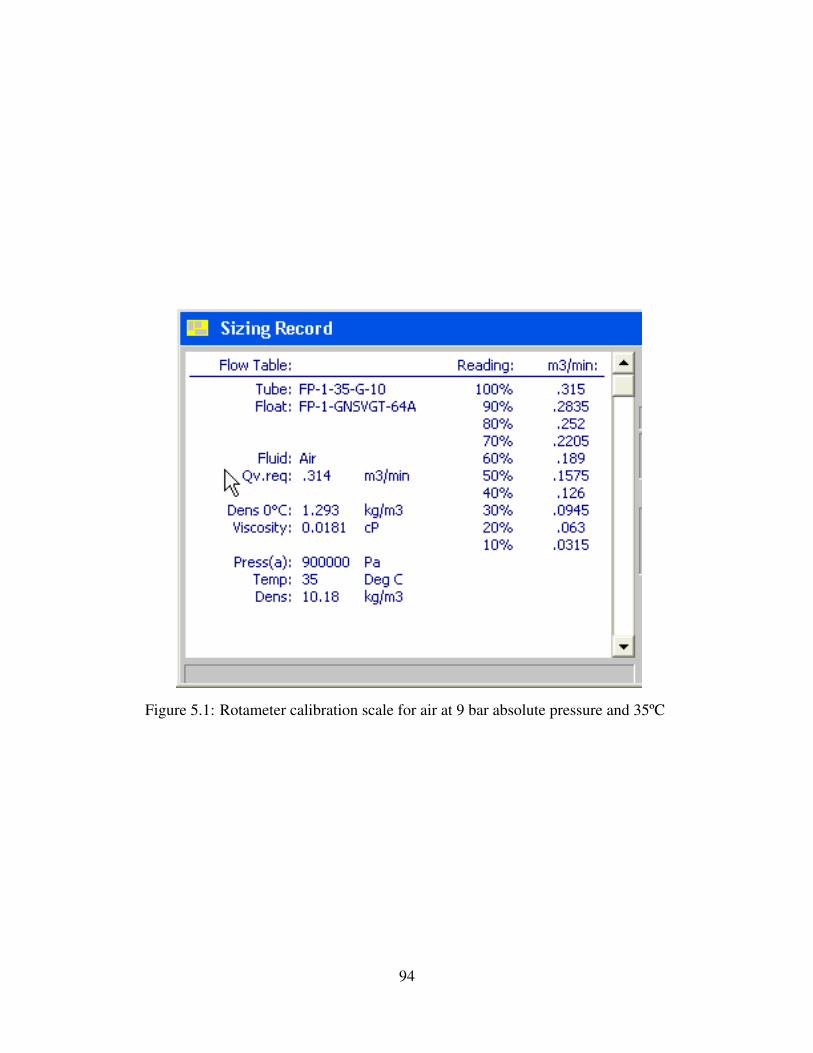
Figure 5.1: Rotameter calibration scale for air at 9 bar absolute pressure and 35ºC
94
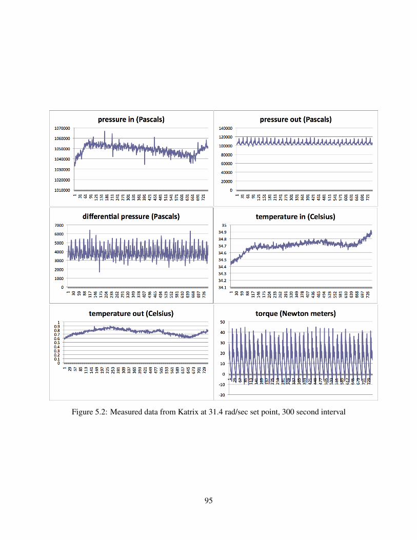
Figure 5.2: Measured data from Katrix at 31.4 rad/sec set point, 300 second interval
95
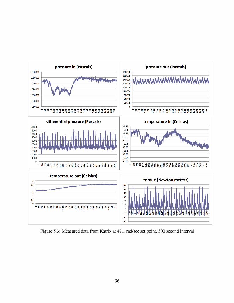
Figure 5.3: Measured data from Katrix at 47.1 rad/sec set point, 300 second interval
96
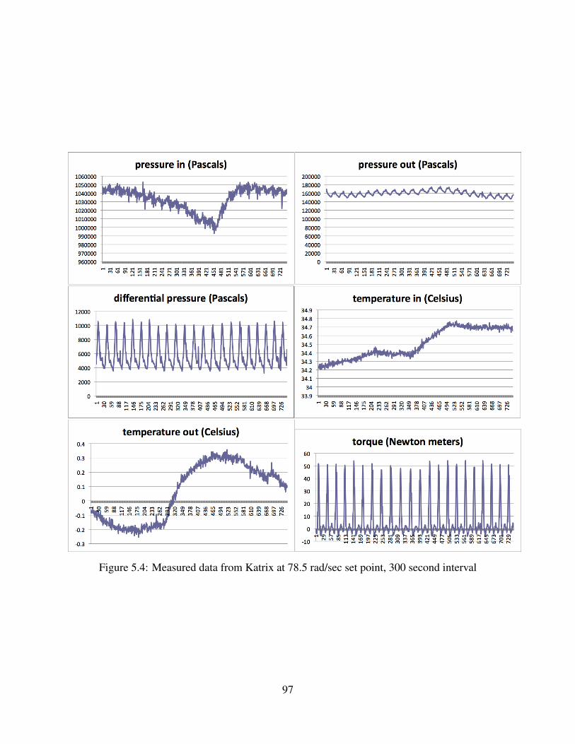
Figure 5.4: Measured data from Katrix at 78.5 rad/sec set point, 300 second interval
97
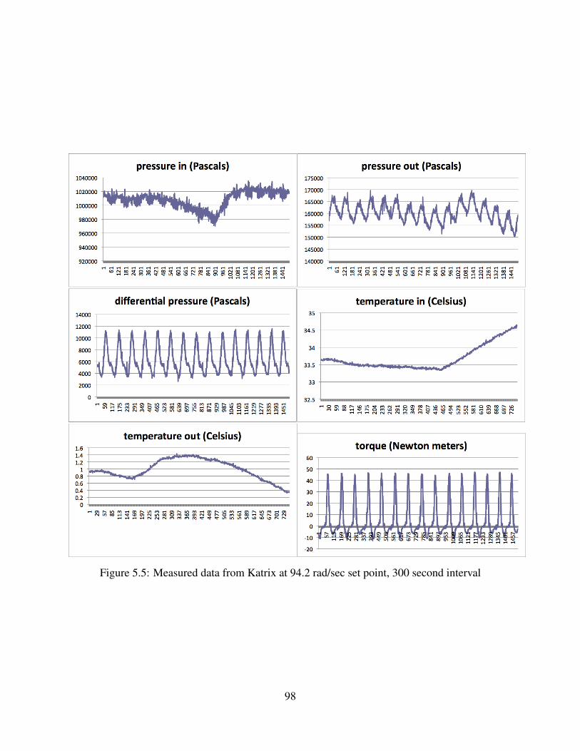
Figure 5.5: Measured data from Katrix at 94.2 rad/sec set point, 300 second interval
98
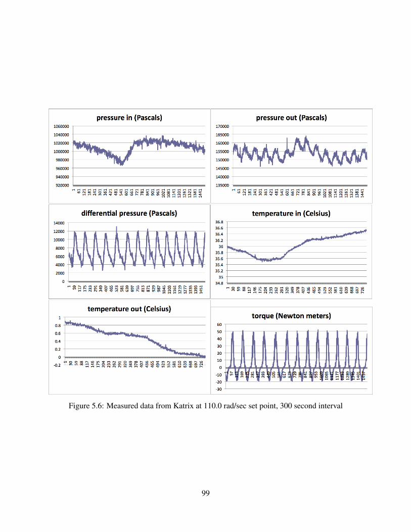
Figure 5.6: Measured data from Katrix at 110.0 rad/sec set point, 300 second interval
99

Figure 5.7: Measured data from Katrix at 125.7 rad/sec set point, 300 second interval
100
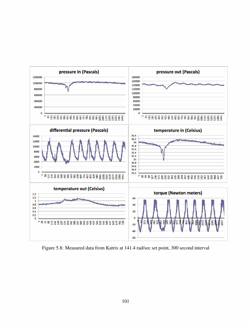
Figure 5.8: Measured data from Katrix at 141.4 rad/sec set point, 300 second interval
101

Chapter 6
Appendix B: Matlab Code for Katrix DataProcessing
102
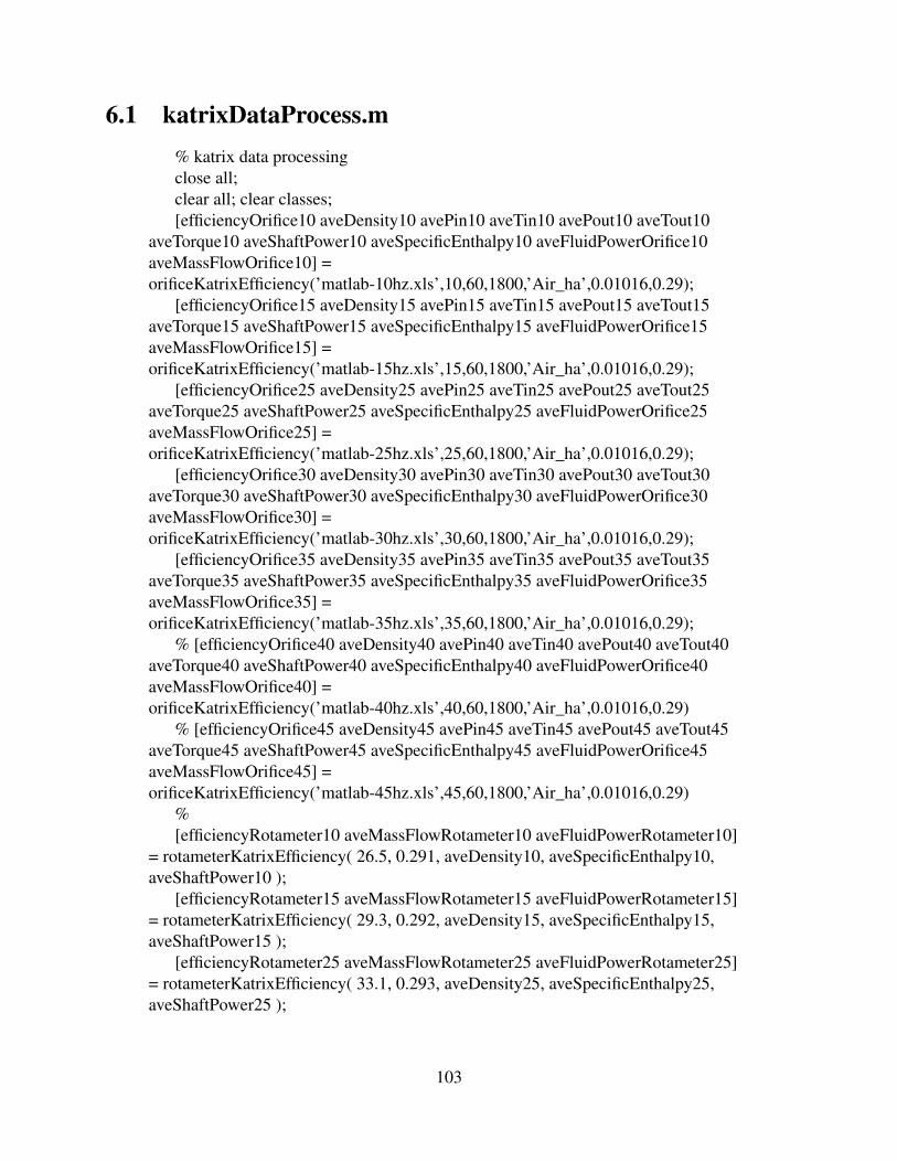
6.1 katrixDataProcess.m% katrix data processingclose all;clear all; clear classes;[efficiencyOrifice10 aveDensity10 avePin10 aveTin10 avePout10 aveTout10
aveTorque10 aveShaftPower10 aveSpecificEnthalpy10 aveFluidPowerOrifice10aveMassFlowOrifice10] =orificeKatrixEfficiency(’matlab-10hz.xls’,10,60,1800,’Air_ha’,0.01016,0.29);
[efficiencyOrifice15 aveDensity15 avePin15 aveTin15 avePout15 aveTout15aveTorque15 aveShaftPower15 aveSpecificEnthalpy15 aveFluidPowerOrifice15aveMassFlowOrifice15] =orificeKatrixEfficiency(’matlab-15hz.xls’,15,60,1800,’Air_ha’,0.01016,0.29);
[efficiencyOrifice25 aveDensity25 avePin25 aveTin25 avePout25 aveTout25aveTorque25 aveShaftPower25 aveSpecificEnthalpy25 aveFluidPowerOrifice25aveMassFlowOrifice25] =orificeKatrixEfficiency(’matlab-25hz.xls’,25,60,1800,’Air_ha’,0.01016,0.29);
[efficiencyOrifice30 aveDensity30 avePin30 aveTin30 avePout30 aveTout30aveTorque30 aveShaftPower30 aveSpecificEnthalpy30 aveFluidPowerOrifice30aveMassFlowOrifice30] =orificeKatrixEfficiency(’matlab-30hz.xls’,30,60,1800,’Air_ha’,0.01016,0.29);
[efficiencyOrifice35 aveDensity35 avePin35 aveTin35 avePout35 aveTout35aveTorque35 aveShaftPower35 aveSpecificEnthalpy35 aveFluidPowerOrifice35aveMassFlowOrifice35] =orificeKatrixEfficiency(’matlab-35hz.xls’,35,60,1800,’Air_ha’,0.01016,0.29);
% [efficiencyOrifice40 aveDensity40 avePin40 aveTin40 avePout40 aveTout40aveTorque40 aveShaftPower40 aveSpecificEnthalpy40 aveFluidPowerOrifice40aveMassFlowOrifice40] =orificeKatrixEfficiency(’matlab-40hz.xls’,40,60,1800,’Air_ha’,0.01016,0.29)
% [efficiencyOrifice45 aveDensity45 avePin45 aveTin45 avePout45 aveTout45aveTorque45 aveShaftPower45 aveSpecificEnthalpy45 aveFluidPowerOrifice45aveMassFlowOrifice45] =orificeKatrixEfficiency(’matlab-45hz.xls’,45,60,1800,’Air_ha’,0.01016,0.29)
%[efficiencyRotameter10 aveMassFlowRotameter10 aveFluidPowerRotameter10]
= rotameterKatrixEfficiency( 26.5, 0.291, aveDensity10, aveSpecificEnthalpy10,aveShaftPower10 );
[efficiencyRotameter15 aveMassFlowRotameter15 aveFluidPowerRotameter15]= rotameterKatrixEfficiency( 29.3, 0.292, aveDensity15, aveSpecificEnthalpy15,aveShaftPower15 );
[efficiencyRotameter25 aveMassFlowRotameter25 aveFluidPowerRotameter25]= rotameterKatrixEfficiency( 33.1, 0.293, aveDensity25, aveSpecificEnthalpy25,aveShaftPower25 );
103

[efficiencyRotameter30 aveMassFlowRotameter30 aveFluidPowerRotameter30]= rotameterKatrixEfficiency( 34.2, 0.296, aveDensity30, aveSpecificEnthalpy30,aveShaftPower30 );
[efficiencyRotameter35 aveMassFlowRotameter35 aveFluidPowerRotameter35]= rotameterKatrixEfficiency( 35.7, 0.297, aveDensity35, aveSpecificEnthalpy35,aveShaftPower35 );
% [efficiencyRotameter40 aveMassFlowRotameter40aveFluidPowerRotameter40] = rotameterKatrixEfficiency( 37.7, 0.296,aveDensity40, aveSpecificEnthalpy40, aveShaftPower40 )
% [efficiencyRotameter45 aveMassFlowRotameter45aveFluidPowerRotameter45] = rotameterKatrixEfficiency( 39.0, 0.30, aveDensity45,aveSpecificEnthalpy45, aveShaftPower45 )
rotationalSpeed = [300 450 750 900 1050].*(2*pi/60); % rpm to rad/secondnumSamples = length(rotationalSpeed);efficiencyOrifice = [efficiencyOrifice10 efficiencyOrifice15 efficiencyOrifice25
efficiencyOrifice30 efficiencyOrifice35 ];efficiencyRotameter = [efficiencyRotameter10 efficiencyRotameter15
efficiencyRotameter25 efficiencyRotameter30 efficiencyRotameter35 ];fluidPowerOrifice = [aveFluidPowerOrifice10 aveFluidPowerOrifice15
aveFluidPowerOrifice25 aveFluidPowerOrifice30 aveFluidPowerOrifice35 ];fluidPowerRotameter = [aveFluidPowerRotameter10 aveFluidPowerRotameter15
aveFluidPowerRotameter25 aveFluidPowerRotameter30 aveFluidPowerRotameter35];
massFlowOrifice = [aveMassFlowOrifice10 aveMassFlowOrifice15aveMassFlowOrifice25 aveMassFlowOrifice30 aveMassFlowOrifice35 ];
massFlowRotameter = [aveMassFlowRotameter10 aveMassFlowRotameter15aveMassFlowRotameter25 aveMassFlowRotameter30 aveMassFlowRotameter35 ];
shaftPower = [aveShaftPower10 aveShaftPower15 aveShaftPower25aveShaftPower30 aveShaftPower35 ];
Torque = [aveTorque10 aveTorque15 aveTorque25 aveTorque30 aveTorque35 ];Pin = [avePin10 avePin15 avePin25 avePin30 avePin35 ];Pout = [avePout10 avePout15 avePout25 avePout30 avePout35 ];Tin = [aveTin10 aveTin15 aveTin25 aveTin30 aveTin35 ] + 273.15;% Celsius to
KelvinTout = [aveTout10 aveTout15 aveTout25 aveTout30 aveTout35 ] + 273.15;%
Celsius to KelvinspecificEnthalpy = [aveSpecificEnthalpy10 aveSpecificEnthalpy15
aveSpecificEnthalpy25 aveSpecificEnthalpy30 aveSpecificEnthalpy35 ];Pratio = Pin./Pout;meanEfficiency = mean([efficiencyOrifice; efficiencyRotameter]);meanFluidPower = mean([fluidPowerOrifice; fluidPowerRotameter]);meanMassFlow = mean([massFlowOrifice; massFlowRotameter]);
104

stdDevEfficiency = std([efficiencyOrifice; efficiencyRotameter], 1, 1); %onestandard deviation based on 2 independent data points, orifice and rotameter
stdDevFluidPower = std([fluidPowerOrifice; fluidPowerRotameter], 1, 1); %onestandard deviation based on 2 independent data points, orifice and rotameter
stdDevMassFlow = std([massFlowOrifice; massFlowRotameter], 1, 1); %onestandard deviation based on 2 independent data points, orifice and rotameter
accuracyTorque = (0.0025*50).*ones(1,numSamples); % Interface T8-50-A4A,T8-Eco w/ 50 Nm capacity, +/-0.25% combined accuracy
accuracyShaftPower = (accuracyTorque./Torque + 0.01).*shaftPower; %Multiplication, Power = Torque*angular velocity, so add relative error. YaskawaV1000, +/-1.0% speed regulation in V/f mode
accuracyPin = (0.01*1825042).*ones(1,numSamples); % PX26-250GV, +/-1.0%accuracy, 250psig capacity
accuracyPout = (0.003*2169780).*ones(1,numSamples); % PX181-300G5V,+/-0.3% combined accuracy, 300psig capacity
accuracyTin = 2.2.*ones(1,numSamples); % Omega TJ36-CAXL-18G-6grounded, type K thermocouple, 2.2 degree ASTM tolerance
accuracyTout = accuracyTin; % Omega TJ36-CAXL-18G-6 grounded, type Kthermocouple, ASTM tolerance
accuracyPratio = (accuracyPin./Pin + accuracyPout./Pout).*Pratio; % Division, soadd relative error
figure();errorbar(rotationalSpeed,meanEfficiency,stdDevEfficiency,’o–’);axis([0, 120, 0.5 , 1]);ylabel(’Isentropic efficiency’);xlabel(’Rotational speed (radians/second)’);figure();errorbar(rotationalSpeed,meanFluidPower,stdDevFluidPower,’o–’);hold on;errorbar(rotationalSpeed,shaftPower,accuracyShaftPower,’–’);axis([0, 120, 0 , 700]);ylabel(’Power (Joules/second)’);xlabel(’Rotational speed (radians/second)’);legend(’Enthalpy loss of air through expander’, ’Mechanical power generated’,
’Location’, ’Best’);figure();errorbar(rotationalSpeed,Torque,accuracyTorque,’–’);axis([0, 120, 0 , 15]);ylabel(’Average torque produced (Newton*meter)’);xlabel(’Rotational speed (radians/second)’);figure();errorbar(rotationalSpeed,Pratio,accuracyPratio,’–’);axis([0, 120, 0 , 11]);
105
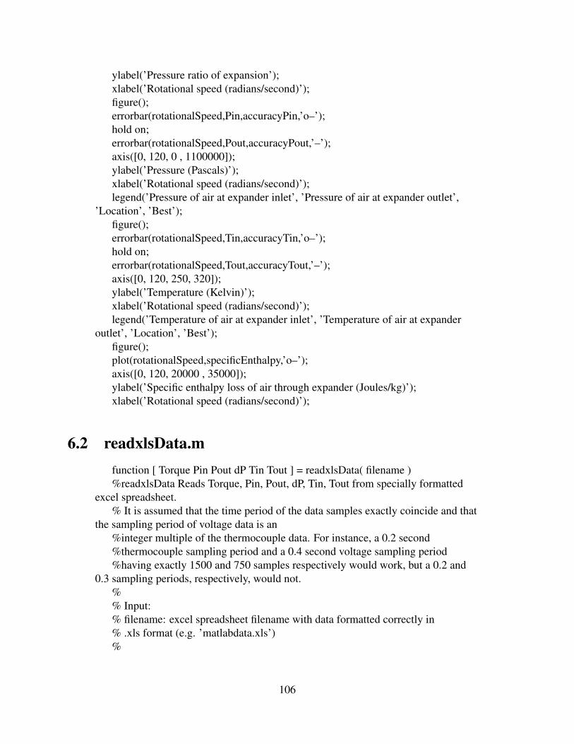
ylabel(’Pressure ratio of expansion’);xlabel(’Rotational speed (radians/second)’);figure();errorbar(rotationalSpeed,Pin,accuracyPin,’o–’);hold on;errorbar(rotationalSpeed,Pout,accuracyPout,’–’);axis([0, 120, 0 , 1100000]);ylabel(’Pressure (Pascals)’);xlabel(’Rotational speed (radians/second)’);legend(’Pressure of air at expander inlet’, ’Pressure of air at expander outlet’,
’Location’, ’Best’);figure();errorbar(rotationalSpeed,Tin,accuracyTin,’o–’);hold on;errorbar(rotationalSpeed,Tout,accuracyTout,’–’);axis([0, 120, 250, 320]);ylabel(’Temperature (Kelvin)’);xlabel(’Rotational speed (radians/second)’);legend(’Temperature of air at expander inlet’, ’Temperature of air at expander
outlet’, ’Location’, ’Best’);figure();plot(rotationalSpeed,specificEnthalpy,’o–’);axis([0, 120, 20000 , 35000]);ylabel(’Specific enthalpy loss of air through expander (Joules/kg)’);xlabel(’Rotational speed (radians/second)’);
6.2 readxlsData.mfunction [ Torque Pin Pout dP Tin Tout ] = readxlsData( filename )%readxlsData Reads Torque, Pin, Pout, dP, Tin, Tout from specially formatted
excel spreadsheet.% It is assumed that the time period of the data samples exactly coincide and that
the sampling period of voltage data is an%integer multiple of the thermocouple data. For instance, a 0.2 second%thermocouple sampling period and a 0.4 second voltage sampling period%having exactly 1500 and 750 samples respectively would work, but a 0.2 and
0.3 sampling periods, respectively, would not.%% Input:% filename: excel spreadsheet filename with data formatted correctly in% .xls format (e.g. ’matlabdata.xls’)%
106
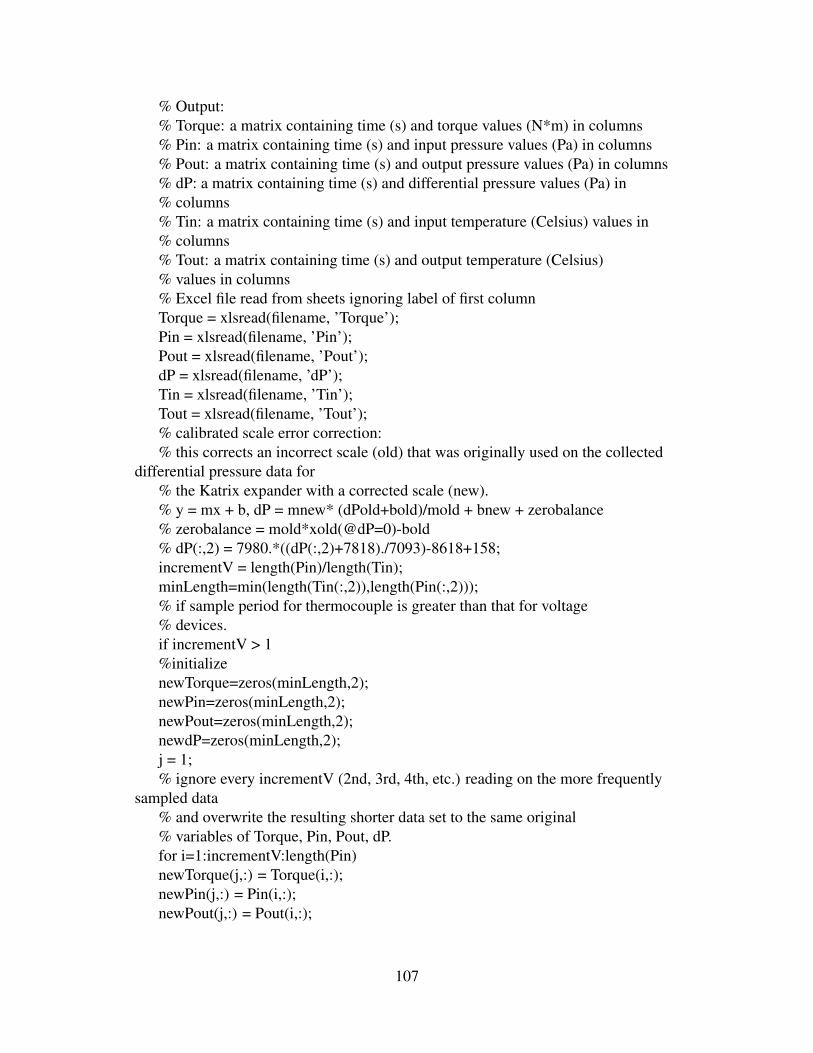
% Output:% Torque: a matrix containing time (s) and torque values (N*m) in columns% Pin: a matrix containing time (s) and input pressure values (Pa) in columns% Pout: a matrix containing time (s) and output pressure values (Pa) in columns% dP: a matrix containing time (s) and differential pressure values (Pa) in% columns% Tin: a matrix containing time (s) and input temperature (Celsius) values in% columns% Tout: a matrix containing time (s) and output temperature (Celsius)% values in columns% Excel file read from sheets ignoring label of first columnTorque = xlsread(filename, ’Torque’);Pin = xlsread(filename, ’Pin’);Pout = xlsread(filename, ’Pout’);dP = xlsread(filename, ’dP’);Tin = xlsread(filename, ’Tin’);Tout = xlsread(filename, ’Tout’);% calibrated scale error correction:% this corrects an incorrect scale (old) that was originally used on the collected
differential pressure data for% the Katrix expander with a corrected scale (new).% y = mx + b, dP = mnew* (dPold+bold)/mold + bnew + zerobalance% zerobalance = mold*xold(@dP=0)-bold% dP(:,2) = 7980.*((dP(:,2)+7818)./7093)-8618+158;incrementV = length(Pin)/length(Tin);minLength=min(length(Tin(:,2)),length(Pin(:,2)));% if sample period for thermocouple is greater than that for voltage% devices.if incrementV > 1%initializenewTorque=zeros(minLength,2);newPin=zeros(minLength,2);newPout=zeros(minLength,2);newdP=zeros(minLength,2);j = 1;% ignore every incrementV (2nd, 3rd, 4th, etc.) reading on the more frequently
sampled data% and overwrite the resulting shorter data set to the same original% variables of Torque, Pin, Pout, dP.for i=1:incrementV:length(Pin)newTorque(j,:) = Torque(i,:);newPin(j,:) = Pin(i,:);newPout(j,:) = Pout(i,:);
107
newdP(j,:) = dP(i,:);j = j+1;endTorque = newTorque;Pin = newPin;Pout = newPout;dP = newdP;% if sample period for thermocouple is less than that for voltage% data.elseif incrementV < 1% initializenewTin=zeros(minLength,2);newTout=zeros(minLength,2);j = 1;% ignore every incrementV (2nd, 3rd, 4th, etc.) reading on the more frequently
sampled data% and overwrite the resulting shorter data set to the same original% variables of Tin, Tout.for i=1:(1/incrementV):length(Tin)newTin(j,:) = Tin(i,:);newTout(j,:) = Tout(i,:);j = j+1;endTin = newTin;Tout = newTout;endend
6.3 orificeKatrixEfficiency.mfunction [ efficiencyOrifice aveDensity avePin aveTin avePout aveTout aveTorque
aveShaftPower aveSpecificEnthalpy aveFluidPower aveMassFlow] =orificeKatrixEfficiency( filename, frequency, basefrequency, ratedrpm, workingfluid,d, orificeRatio)
%katrixEfficiency computes the expander isentropic efficiency, average fluiddensity,
%pressure in, temperature in, pressure out, temperature out, torque, shaft power,%fluid power, and mass flow rate from experimental data stored in specially
formatted excel spreadsheets.%Flow rate is calculated using data from an orifice plate flow meter, and%using the Blevins orifice equation. It is assumed that the time period of
108
%the data samples exactly coincide and that the sampling period of voltage datais an
%integer multiple of the thermocouple data. For instance, a 0.2 second%thermocouple sampling period and a 0.4 second voltage sampling period%having exactly 1500 and 750 samples respectively would work, but a 0.2 and
0.3 sampling periods, respectively, would not.%% Variables;%% Output:% efficiencyOrifice: average isentropic efficiency of expander (0 = 0%, 1 = 100%)% aveDensity: average density of working fluid upstream of expander% (kg/m^3)% avePin: average pressure upstream (Pa)% aveTin: average temperature upstream (Celsius)% avePout: average pressure downstream (Pa)% aveTout: average temperature downstream (Celsius)% aveTorque: average torque produced on shaft (N*m)% aveShaftPower: average power produced on shaft (J/s)% aveSpecificEnthalpy: average specific enthalpy loss across expander% (J/kg)% aveFluidPower: average fluid enthalpy loss expressed as power (J/s)% aveMassFlow: average mass flow rate into the expander (kg/s)%% Input:% filename: excel spreadsheet filename with data formatted correctly in% .xls format (e.g. ’matlabdata.xls’)% frequency: AC frequency provided to induction motor/generator (Hz)% baseFrequency: motor nameplate frequency of excitation (Hz)% ratedrpm: motor rated speed at nameplate frequency (Hz)% workingFluid: EES recognized name of working fluid (e.g. ’Air_ha’)% d: diameter of orifice in orifice plate flow meter (m)% orificeRatio: ratio of diameter of orifice to pipe diameter[Torque Pin Pout dP Tin Tout] = readxlsData(filename);% Initial value of the velocity of the fluid through the pipe% upstream of the orifice. This will iteratively be solved, so need% not be correct.U = 2; % m/s% InitializespecificEnthalpy=zeros(minLength,1);viscosity=zeros(minLength,1);density=zeros(minLength,1);mdot=zeros(minLength,1);
109

fluidPower=zeros(minLength,1);shaftPower=zeros(minLength,1);% Calculate the instantaneous power, enthalpyloss, mass flow, etc. for each% time step in the data set using the EES/matlab interface.for i=1:1:length(Tin)% Calculate the shaftpower (converting from rpm to rad/secshaftPower(i) = 2*pi/60 * frequency / basefrequency * ratedrpm * Torque(i,2);% Calculate specific enthalpy drop in fluid across expander.specificEnthalpy(i) = EES_Enthalpy(workingfluid,’P’,Pin(i,2),’T’,Tin(i,2)) -
EES_Enthalpy(workingfluid,’P’,Pout(i,2),’T’,Tout(i,2));% Calculate density of fluid in upstream flow.density(i) = EES_Density( workingfluid, ’P’, Pin(i,2), ’T’, Tin(i,2));% Calculate viscosity of fluid in upstream flow.viscosity(i) = EES_Viscosity( workingfluid, ’P’, Pin(i,2), ’T’, Tin(i,2));% Using an iterative algorithm with the Blevins incompressible flow correlation,
calculate the mass% flow rate based on the orifice plate differential pressure reading and a velocity
guess.mdot(i) = Blevins(d,orificeRatio,density(i),viscosity(i),dP(i,2),U);% Calculate the total enthalpy drop of fluid across the expander.fluidPower(i) = mdot(i)*specificEnthalpy(i);end% calculate average values (across the whole dataset) of the above% calculated instantaneous values.avePin = mean(Pin(:,2));aveTin = mean(Tin(:,2));avePout = mean(Pout(:,2));aveTout = mean(Tout(:,2));aveTorque = mean(Torque(:,2));aveShaftPower = mean(shaftPower);aveSpecificEnthalpy = mean(specificEnthalpy);aveFluidPower = mean(fluidPower);aveDensity = mean(density);aveMassFlow = mean(mdot);% average isentropic efficiency across this dataset.efficiencyOrifice = aveShaftPower/aveFluidPower;end
6.4 Blevins.mfunction [ mdot ] = Blevins( d, beta, rho, mu, dP, U )% Blevins mass flow rate for orifice plate with corner tap, incompressible
110
% fluid% source: Blevins Applied Fluid Dynamics Handbook.%% Variables:%% Output% mdot: mass flow rate (kg/s)%% Input% d: diameter of orifice (m)% beta: ratio of diameter of orifice to inner diameter of pipe% rho: density of working fluid upstream of orifice (kg/m^3)% mu: viscosity of working fluid upstream of orifice% dP: differential pressure across the orifice (corner flange)% U: velocity of air through the pipe% orifice outer diameterD = d/beta;% start with a high mdotdelta to enter the while loop.mdotdelta = 0.02;% assume zero mass flow so at least two iterations are always performed in% while loop.mdotlast = 0;while mdotdelta > 0.0001% Reynolds number of flow through upstream pipeRe = rho*U*D/mu;% Blevins 6-40, calculation of discharge coefficient to account for% viscous lossesC = 0.5959 + 0.0312*beta^2.1 - 0.1840*beta^8 + 91.71*beta^2.5*Re^(-0.75);% Blevins 6-39, calculation of mass flow ratemdot = (rho*pi*d^2*C/(4*(1-(beta)^4)^0.5)*(2*dP/rho)^0.5); %kg/sU = mdot/rho/(pi*(D/2)^2); % m/s% calculation of difference between this and previous iterations mdot% result.mdotdelta = mdot - mdotlast;% this mdot becomes the previous before returning to the while loop% conditionmdotlast = mdot;endend
111
6.5 rotameterKatrixEfficiency.mfunction [ rotameterEfficiency mdot fluidPower ] = rotameterKatrixEfficiency(
percentMeasured, highLimit, rho, specificEnthalpy, shaftPower)%rotameterKatrixEfficiency calculates mass flow rate based on rotameter.% Using an upstream rotameter with a maximum capacity measured in% m^3/min, calculates the fluidPower and efficiency of the katrix expander given% also the average shaft power produced and density and specific enthalpy of the% air through the rotameter at the time of the reading (steady state).%% Variables:%% Output% rotameterEfficiency: isentropic efficiency of the expander (0 = 0%, 1 =% 100%)% mdot: mass flow rate of working fluid (kg/s)% fluidPower: enthalpy loss of working fluid through expander (J/s)%% Input% percentMeasured: flow as percent of scale measured on rotameter (%)% highLimit: volumeteric flow capacity (100% of scale) of rotameter (m^3/min)% rho: average density of working fluid through rotameter (kg/m^3)% specificEnthalpy: average specific enthalpy drop of fluid through expander
(J/kg)% shaftPower: average shaft power produced by expander (J/s)% measurement * capacity * density (converted to kg/s)mdot = percentMeasured/100 * highLimit * rho / 60;fluidPower = specificEnthalpy * mdot;%isentropic efficiency of expander based on average rotameter readingrotameterEfficiency = shaftPower/fluidPower;end
6.6 dpTorquePlot.mclose all; clear all; clear classes;[Torque10 Pin10 Pout10 dP10 Tin10 Tout10] = readxlsData(’matlab-10hz.xls’);[Torque15 Pin15 Pout15 dP15 Tin15 Tout15] = readxlsData(’matlab-15hz.xls’);[Torque25 Pin25 Pout25 dP25 Tin25 Tout25] = readxlsData(’matlab-25hz.xls’);[Torque30 Pin30 Pout30 dP30 Tin30 Tout30] = readxlsData(’matlab-30hz.xls’);[Torque35 Pin35 Pout35 dP35 Tin35 Tout35] = readxlsData(’matlab-35hz.xls’);[Torque40 Pin40 Pout40 dP40 Tin40 Tout40] = readxlsData(’matlab-40hz.xls’);[Torque45 Pin45 Pout45 dP45 Tin45 Tout45] = readxlsData(’matlab-45hz.xls’);
112
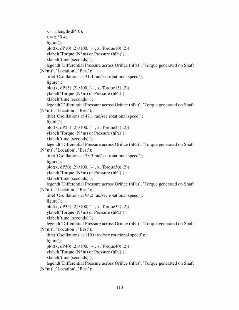
x = 1:length(dP10);x = x.*0.4;figure();plot(x, dP10(:,2)./100, ’–’, x, Torque10(:,2))ylabel(’Torque (N*m) or Pressure (hPa)’);xlabel(’time (seconds)’);legend(’Differential Pressure across Orifice (hPa)’, ’Torque generated on Shaft
(N*m)’, ’Location’, ’Best’);title(’Oscillations at 31.4 rad/sec rotational speed’);figure();plot(x, dP15(:,2)./100, ’–’, x, Torque15(:,2))ylabel(’Torque (N*m) or Pressure (hPa)’);xlabel(’time (seconds)’);legend(’Differential Pressure across Orifice (hPa)’, ’Torque generated on Shaft
(N*m)’, ’Location’, ’Best’);title(’Oscillations at 47.1 rad/sec rotational speed’);figure();plot(x, dP25(:,2)./100, ’–’, x, Torque25(:,2))ylabel(’Torque (N*m) or Pressure (hPa)’);xlabel(’time (seconds)’);legend(’Differential Pressure across Orifice (hPa)’, ’Torque generated on Shaft
(N*m)’, ’Location’, ’Best’);title(’Oscillations at 78.5 rad/sec rotational speed’);figure();plot(x, dP30(:,2)./100, ’–’, x, Torque30(:,2))ylabel(’Torque (N*m) or Pressure (hPa)’);xlabel(’time (seconds)’);legend(’Differential Pressure across Orifice (hPa)’, ’Torque generated on Shaft
(N*m)’, ’Location’, ’Best’);title(’Oscillations at 94.2 rad/sec rotational speed’);figure();plot(x, dP35(:,2)./100, ’–’, x, Torque35(:,2))ylabel(’Torque (N*m) or Pressure (hPa)’);xlabel(’time (seconds)’);legend(’Differential Pressure across Orifice (hPa)’, ’Torque generated on Shaft
(N*m)’, ’Location’, ’Best’);title(’Oscillations at 110.0 rad/sec rotational speed’);figure();plot(x, dP40(:,2)./100, ’–’, x, Torque40(:,2))ylabel(’Torque (N*m) or Pressure (hPa)’);xlabel(’time (seconds)’);legend(’Differential Pressure across Orifice (hPa)’, ’Torque generated on Shaft
(N*m)’, ’Location’, ’Best’);
113

title(’Oscillations at 125.7 rad/sec rotational speed’);figure();plot(x, dP45(:,2)./100, ’–’, x, Torque45(:,2))ylabel(’Torque (N*m) or Pressure (hPa)’);xlabel(’time (seconds)’);legend(’Differential Pressure across Orifice (hPa)’, ’Torque generated on Shaft
(N*m)’, ’Location’, ’Best’);title(’Oscillations at 141.4 rad/sec rotational speed’);frequency = [34 31 22 15 13 12 9]./300; % number of periods in 300 secondsrotationalSpeed = [300 450 750 900 1050 1200 1350].*(2*pi/60); % rpm to
rad/secondfigure();plot(rotationalSpeed, frequency, ’o–’)axis([0, 160, 0 , 0.12]);ylabel(’Frequency of Oscillation (Hz)’);xlabel(’Rotational Speed (rad/second)’);
114