A behavioral study of gabion retaining walls

Item Type text; Dissertation-Reproduction (electronic)

Authors Sublette, William Robert

Publisher The University of Arizona.

Rights Copyright © is held by the author. Digital access to this materialis made possible by the University Libraries, University of Arizona.Further transmission, reproduction or presentation (such aspublic display or performance) of protected items is prohibitedexcept with permission of the author.

Download date 13/05/2018 00:24:19

Link to Item http://hdl.handle.net/10150/565450

A BEHAVIORAL STUDY OF GABION RETAINING WALLS

byWilliam Robert Sublette

A Dissertation Submitted to the Faculty of theDEPARTMENT OF CIVIL ENGINEERING AND

ENGINEERING MECHANICSIn Partial Fulfillment of the Requirements

For the Degree of. "DOCTOR • OF PHILOSOPHY

WITH A MAJOR IN CIVIL ENGINEERINGIn the Graduate College

THE UNIVERSITY OF ARIZONA

1 9 7 9

THE UNIVERSITY OF ARIZONA GRADUATE COLLEGE

I hereby recommend that this dissertation prepared under my direction by _____________________William Robert Subletteentitled A Behavioral Study of Gabion

Retaining Wallsbe accepted as fulfilling the dissertation requirement for the Degree of ______________________ Doctor of Philosophy

As members of the Final Examination Committee, we certify that we have read this dissertation and agree that it may be presented for final defense.

/ 0. ____ __' /l ) / / 0 Date(f?i J-'JY--------------------- c J / W ? ? -------

Date

Date

Date

Final approval and acceptance of this dissertation is contingent on the candidate's adequate performance and defense thereof at the final oral examination.

STATEMENT BY AUTHOR

. This .dissertation has been submitted in partial fulfillment of requirements for an advanced degree at The University of Arizona and is deposited in the University Library to be made available to borrowers under rules of the Library.

Brief, quotations from this dissertation are allow­able without special permission, provided that accurate acknowledgment of source is made. Requests for permission for extended quotation from or reproduction of this manu­script in whole or in part may be granted by the head of the major department or the Dean of the Graduate College when in his judgment the proposed use of the material is in the interests of scholarship. In all other instances, however, permission must be obtained from the author.

SIGNED: %

ACKNOWLE DGMEN T\

I wish to express my sincere appreciation to my dissertation director. Dr. Hassan A. Sultan, for his very helpful guidance and encouragement throughout my research.

Special appreciation is due Dr. Robert L. Sogge for his assistance in the initial phase of the research.

I wish to also thank Dr. Ralph M. Richard for pro­viding his professional experience for the solution of prob­lems encountered in finite element modeling.

Additional gratitude is extended to Dr. Edward A. Nowatzki for reviewing the study and his continued encourage­ment throughout the research.

Thanks are also given to Bal K . Sanan for the helpful discussions involving problems encountered in the research, and to Zena HIobi1 for her review of the first draft.

iii

TABLE OF CONTENTS

LIST OF ILLUSTRATIONS . . . . . . . . . . . . . . . viLIST OF TABLES ................................... ixABSTRACT . . . . . . . . . . . . . . . . . . . . . x

1. INTRODUCTION . . . . . . . . . . . 1Description of Gabion Box ..................... 3Versatility of Gabion Boxes .................. 7Description of Gabion Retaining Wall . . . . . 9Soil-structure Interactions of theRetaining Wall . . . . . . . . 13

Objective and Scope of Research .............. 142. REVIEW OF EXPERIENCE WITH GABION

RETAINING WALLS . . . . . . . . . . . . . . . . . 16Advantages of Gabion Retaining Walls ........ 18Description of Conventional Design Method . . . 20Limitations of Conventional Design Method . . . 21

3. FINITE ELEMENT P R O G R A M ............ . 22Capabilities.............. . 22Modifications and Additions . . ............... 23

4. MATERIAL CHARACTERIZATION FOR A N A L Y S I S......... 27Soil Model ................................... 27'

No Tension Characteristics . . . . . . . . 31Wire Mesh Model . 33

No-compression Characteristics . . . . . . 38Connecting Wire Model . . . . . . 40

5. FINITE ELEMENT MODELING . . . . 41Wire Mesh Modeling ....................... 41Single Gabion Box Modeling .................. 42Modeling 12 ft. Gabion Retaining W a l l ........ 48Modeling 45 ft. Gabion Retaining Wall . . . . . 56

Page

iv

V

TABLE OF CONTENTS, Continued.

6. PRESENTATION AND DISCUSSION OF FINITEELEMENT ANALYSTS RESULTS ....................... 67Wire Mesh ............................. 67Gabion Box ............................... .. . 6912 ft. Gabion Retaining W a l l .......... .. . . 76

Finite Element Versus Conventional' Stability Analysis . 91

45 ft. Gabion Retaining Wall'.......... 937. DEVELOPMENT OF CONSTITUTIVE EQUATIONS

FOR A GABION BOX ............................... 968. CONCLUSIONS AND RECOMMENDATIONS ................ 99

Conclusions . . . . . . . . 99Design Applications . 102Recommendations for Further Research . . . . . 104

APPENDIX A: CONVENTIONAL. STABILITY ANALYSISOF A 12 FT. GABION RETAININGWALL 106

APPENDIX B: WIRE MESH NONLINEAR STRESS-STRAINELASTIC-PLASTIC FITTING METHOD. . . 113

APPENDIX C: FINITE ELEMENT STABILITY ANALYSISOF A 12 FT. GABION RETAININGW A L L .................. ' . . . . 121

APPENDIX D: DETAILS OF CONSTITUTIVE EQUATIONDEVELOPMENT FOR GABION BOX . . . . 126

Page

LIST OF REFERENCES 138

LIST OF ILLUSTRATIONS

1.1 Unfabricated and Fabricated Gabion BoxFormed with a Hexagonal Steel Wire Mesh . . . 4

1.2 Wire Mesh Components of the Gabion Box . . . . 51.3 Typical Hexagonal Dimensions, for.

the Wire Mesh ............................... 61.4 Location and Use of the Connecting Wires

in the Gabion Box ........................... 81.5 Typical Gabion Retaining Wall

Supporting a Mountain R o a d ................ 101.5 Typical Vertical Gabion Retaining Wall

with a Stepped Exterior Face ............... 111.7 Typical Inclined Gabion Retaining Wall

with a Flat Exterior F a c e .................. 124.1 Typical Section of Hexagonal Triple Twisted

Steel Wire Mesh Used in the Gabion Box . . . 344.2 Stress-strain Relationship for Hexagonal

Wire Mesh with Loading Parallel to the Major Principal Dimension of theHexagonal........ .. . . . ............... .. 35

4.3 Stress-strain Relationship for HexagonalWire Mesh with Loading Parallel to the Minor Principal Dimension of theHexagonal ............................... .. . 36

5.1 Finite Element Model of the Gabion Wire Meshwith Loading Applied Parallel to the Major Principal Dimension of theHexagonal ................................. .. 43

5.2 Finite Element Model of the Gabion WireMesh with Loading Applied Parallel to theMinor Principal Dimension of the Hexagonal . 44

Figure Page

■ vi

viiLIST OF ILLUSTRATIONS, Continued.

5.3 Finite Element Model of a SingleGabion Box ............ . . 45

5.4 12 ft. Gabion Retaining Wall . ................. 495.5 Finite Element Model of a 12 ft. Gabion

Retaining Wall and Surrounding Soil . . . . . 50

Figure Page

5.6 Typical Gabion Dimensions andElement Composition ........ ..............5 4

5.7 45 ft. Snoqualmie Pass GabionRetaining Wall ........ ..............57

5.8 Finite Element Model of the 45 ft.Snoqualmie Pass Gabion Retaining Wall . . . . 58

6.1 Nonlinear Variation of Poisson's Ratio with Respect to Strain in a Direction Parallel to the Major Principal Dimen­sion in the Hexagonal Wire Mesh .............70

6.2 Nonlinear Variation of Poisson's Ratio withRespect to Strain in a Direction Parallelto the Minor Principal Dimension in theHexagonal Wire Mesh . ................. .. 71

6.3 Vertical Stress Applied to Top of GabionBox Versus Vertical Strain inGabion Box . . ..................... .. 72

6.4 Vertical Stress Applied to Top of GabionBox Versus Connecting Wire Stress inGabion B o x ........................ .. 75

6.5 Horizontal Deflections for the Exterior Faceof the 12 ft. Retaining W a l l ................ 77

6.6 Horizontal Deflections for the BackFace of the 12 ft. Retaining W a l l .......... 79

Vertical Stress Contour Map of 12 ft.Gabion Retaining Wall and Backfill . . . . . .

6.781

viii

Figure Page

LIST OF ILLUSTRATIONS, Continued.

6.8 Horizontal Stress Contour Map of 12 ft.Gabion Retaining Wall and Backfill . . . . . . 82

6.9 Horizontal Pressure on Back Face of 12 ft.Retaining Wall Versus Wall Elevation ........ 84

6 o 10 Sections through 12 ft. GabionRetaining Wall . . . . . 87

6.11 Connecting Wire Stress Versus WallElevation ............................... .. . 89

6.12 Wire Mesh Stress Versus Wall Elevation . . . . . 906.13 Horizontal Deflections for the Exterior

Face of the 45 ft. Gabion Retaining Wall . . . 95A. 1 12 ft. Gabion Retaining Wall Analyzed

as a Mass Gravity Structure ................. 107B.l A Hypothetical Curve Representing Eq. (4.10) . . 114B.2 Stress-strain Relationship for Hexagonal

Wire Mesh with Loading Parallel to Major Principal Dimension of the Hexagonal ........ 116

B. 3 Stress-strain Relationship for Hexagonal Wire Mesh with Loading Parallel to Minor Principal Dimension of the Hexagonal . . . . . 119

C.l Stress Distribution (K/ft^) on a 12 ft.Gabion Retaining Wall Developed from aFinite Element Analysis . . . . ............ 122

D.l Unit Cell Diagram of a Gabion Box . .'........ 127D.2 Unfabricated Shape of the Unit Cell Gabion

Box Showing the Hexagonal Wire Meshes Geometric Orientations . ..................... 128

Table6.1

LIST OF TABLES

PageFactors of Safety (F.S.) for Conventional

and Finite Element Stability Analysis of the 12 ft. Gabion Retaining W a l l .......... 92

ix

ABSTRACT

The earliest known use of gabion type structures was for bank protection along the Nile River during the era of the Pharaohs of Egypt. In the subsequent 7000 years since its initial use by the Egyptians, the gabion has been imple­mented into the construction of many different types of structures. Recently the use of gabions has been extended to the construction of gabion retaining walls.

The conventional design method presently used to analyze the stability of a gabion retaining wall considers it as a rigid mass gravity structure. . The ,■ conventional de­sign method is limited in that it does not consider the flexibility of the gabion wall nor does it provide an analysis of the soil-structure interaction between the wall and back­fill and also within the gabion box itself. The finite element method provides a means by which these soil-structure interaction problems can be analyzed.

The finite element method was first used to analyze the anisotropic nonlinear stress-strain behavior of the gabion's hexagonal wire mesh. A strain locking effect was observed in the wire meshes' nonlinear stress-strain curve.The nonlinear stress-strain curves were then represented mathematically.

x

xiA single gabion box was also modeled and analyzed

to observe its load-deformation behavior and the develop­ment of stresses in its wire mesh and connecting wires. Following this analysis, 12 ft. and 45 ft. gabion retain­ing walls -were analyzed.

The 12 ft. gabion wall had both the wall and back- fi11 modeled while the 45 ft. gabion wall was so large that only the wall could be modeled due to computer core memory limitations. An attempt was made to model the backfill of the 45 ft. gabion wall with bars having properties of the horizontal subgrade reaction. Due to the unorthodox manner by which the backfill was modeled, the results are question­able.

Condensed five node quadrilateral "Duncan and Chang nonlinear soil model" elements were used to model the 12 ft. wall's backfill soil and gabion wall filler material (cobbles) The wire mesh was modeled as a nonlinear bar element while the connecting wires were modeled as linear bar elements.A no-tension provision was included in the quadrilateral ele­ment while a no-compression provision was incorporated into the bar element.

The results of the 12 ft. gabion wall's analysis were as expected. The wall movements and stress contours showed an active stress state in the backfill soil immediately

xiibehind the wall. This stress redistribution was not the result of arching but the result of a load transfer through vertical shearing brought on by differential movements.

The stress distribution along the back and base of the 12 ft. gabion wall was determined from the results of the finite element analysis. Using these results, the sta­bility of the 12 ft. wall was analyzed and compared with a stability analysis of the wall using the conventional method of analysis. It was generally found that the factors of safety of the finite element stability analysis were less than the factors of safety determined from the conventionalVstability analysis; this indicates that the finite element stability analysis is more conservative.

In an attempt to define the behavior of the gabion mathematically, a set of constitutive equations were devel­oped for a single gabion box. In the future these equations may possibly be used to develop a quadrilateral finite ele­ment which would represent one gabion box.

CHAPTER 1

INTRODUCTION■ ' . 1

In recent years there has been a renewed interest in gabion structures. No doubt some of this interest has been generated by the gabion's environmentally aesthetic features but additional interest is being developed by the versatility and advantages of gabion structures„ This renewed interest is ironic in that the gabion principle has existed for over 7000 years.

The Pharaohs of Egypt used gabion-like structures to build dikes along the Nile about 5000 B.C. Chinese used similar structures along the Yellow River about 1000 B-.C. The Roman Architectus Vitruvius, in his ten books of architecture, written about 20 B.C., described their use as cofferdams. Julius Caesar used them for temporary fortifi­cations during his campaign in Gaul. Later references showed them to be used extensively by the military for Such uses as bunker and gun imp!acement fortifications (Terra Aqua Con­servation , 19 76).

The early gabions, woven from plant fiber, were not very durable. They were adequate for temporary installa­tions, such as field fortifications, but required frequent .

1

2replacement and repair in river control programs. However, because of their versatility and the ease of construction with locally available materials, the gabion principle per­sisted through the centuries. Once the metal wire mesh gabion was developed the durability and therefore life expectancy was increased significantly. Gabions utilizing galvanized wire mesh can have a life expectancy of 40 years or more. A gabion structure built in 1894 on the River Reno at Casalecchio, Italy is still functioning adequately (Agostini et al., 1971). This shows that a gabion structure properly maintained can have a long life expectancy.

Today engineers are being forced to use sites with less than desirable topographical and geological conditions. The gabion unit provides an attractive alternative for con­struction on such undesirable sites. Currently there exists a trend in using these units to support increasingly higher loads and to build them into increasingly higher structures. This trend is approaching the limits of the empirical knowl­edge that is currently available and may soon reach the point of danger. Therefore a fundamental understanding of the basic behavior of these units is needed. This study will involve an analyses of the soil-structure interaction between the wire mesh and soil in the gabion unit box and in the case of the retaining wall the additional soil-structure interac­tion between the soil backfill and the gabion retaining wall.

3Description of Gabion Box

The gabion box'unit is a rectangular cage or basket, divided by diaphragms into cells, and formed of hexagonal triple twisted galvanized steel wire mesh (Fig. 1.1). A polyvinylchloride coating is used to cover the wire mesh on gabions in water environments where the pH level is below 6 or greater than 12 or where a high concentration of organic acids are present. The polyvinylchloride coating also pro­vides greater resistance to abrasion.

The gabion box is fabricated with a front,.back, lid, base, diaphragms and two ends (Fig. 1.2). The gabions are generally received from the manufacturer in bundles with each gabion folded flat. At the job site the gabions are unfolded and the edges are laced together with 3 mm steel wire to form the rec-box (Fig. 1.1). The boxes are then laced to each other as they are placed to form one continuous tied-together structure.

Typical dimens ions for the hexagonal wire mesh are shown in Fig. 1.3. A typical wire diameter for the wire mesh is 3 mm although other wire sizes are available. All the edges of the mesh, including those of the end and diaphragm panels are reinforced with galvanized wire of a greater diam­eter . These selvedge wires, in addition to strengthening the basket, facilitate its assembly and assist in keeping itsquare.

Unfabricated Box Fabricated Box

Fig. 1.1. Unfabricated and Fabricated Gabion Box Formed with a Hexagonal Steel Wire Mesh.(After Agostini et al. , 1971)

Fig. 1.2. Wire Mesh Components of the Gabion Box.(After Maccaferri Gabions, Instructions for Assembly and Erection, n .d.).

6

4 cm

12 cm4 cm

4 cm

Fig. 1.3. Typical Hexagonal Dimensions for the Wire Mesh.

7The material used to fill the gabion boxes is usually

a cobble sized stone ranging from 4 to 8 inches in diameter. Cobbles of this size are too large to pass through the open­ings in the wire mesh. It is normally suggested to use rounded cobbles for the filler material. This is not neces­sary but it will allow for more flexibility in the structure.

The cells in the gabion boxes are filled in one foot layers. This allows for proper compaction and also the installation of 3 mm connecting wires which tie the front of the box with the back of the box (Fig. 1.4). . The use of con­necting wires reduces the amount of bulging in the gabion box itself. Therefore the use of the connecting wire is most effective in those boxes which will have the greatest ten­dency to bulge such as boxes located on the exposed vertical face of a gabion structure. The connecting wires are nor­mally installed in one foot vertical intervals and one foot horizontal intervals using a 3 mm diameter wire.

Versatility of Gabion Boxes Gabion box units are very versatile, and have been

used to construct many different types of structures. This versatility can be attributed to mainly two qualities the gabion box unit has, flexibility and permeability. These two qualities will be discussed later in more detail.

8

Fig. 1.4. Location and Use of the Connecting Wires in the Gabion Box.(After Maccaferri Gabions,Instructions for Assembly and Erection, n.d.)

9Typical gabion box uses are as follows: stream bank

revetments, channel linings, weirs, groins,bridge abutments and wingwalls, culvert headwalls and outlet aprons, offshore breakwaters and beach protection, and retaining walls. It is obvious that the majority of gabion uses have been in water related areas such as stream and ocean structures.

Description of Gabion Retaining Wall The gabion retaining wall (Fig. 1.5) is normally con­

sidered as a rigid mass gravity structure in conventional design procedures. The flexibility of the cobble-wire mesh arrangement is not included in the conventional design con­siderations. Since all the gabion boxes in the retaining

r . - - ■ 'wall are tied with lacing wire to adjoining gabion boxes, the entire gabion wall behaves as a flexible monolithic gravity structure.

Generally two types of wall configurations have been used in the design of,mass gravity gabion retaining walls.One wall configuration is vertical with a stepped exterior face (Fig. 1.6) while a second possible wall configuration is inclined at an angle of approximately 6 degrees arid has a flat exterior face (Fig. 1.7). Tilting the wall 6 degrees towards the backfill moves.the resultant of the earth pres­sure and wall weight away from the toe of the wall and • towards, the center of the base of the wall. This results

10

Fig. 1.5. Typical Gabion Retaining Wall Supporting a Mountain Road.(After Agostini, 1971.)

11

\ / / / \ \\

Fig. 1.6. Typical Vertical Gabion Retaining Wall with a Stepped Exterior Face.

12

Fig 1.7.

/

13in a more uniform pressure on the base of the wall plus an increase in the overturning resisting moment.

When designing gabion walls to retain clay slopes, a system of gabion counterforts is normally recommended. The counterforts serve as drains and as structural members that support the slope by the friction of the bank material against the sides of the counterforts. Hydrostatic pressure in the bank is reduced by the natural permeability of the cobble fi 1 led gabi on's „

Soil-structure Interactions of the Retaining Wall

The soil-structure interaction problem is a very old problem when compared with the relatively short life of geo­technical engineering. The interaction of a retaining wall with a frictional material was treated by Coulomb (1776) and Rankine (1857), and the theories they developed have been continually used with remarkable success in the design of retaining walls.

When utilizing these two theories in the design of a retaining wall only the resultant of the earth pressure acting on the wall of some limiting condition can be determined.These classical earth pressure theories give no information on the deformation of the wall and backfill which is especial­ly important in the analysis of a flexible structure such as a gabion retaining wall.

14The finite element method is ideally suited to deal

with the soil-structure interaction problem of the gabion retaining wall. It provides the opportunity to not only determine the stresses throughout the wall and backfill but also the deformations (Clough, 1972). Even though there are no known finite element analyses of a gabion retaining wall there are a number of soil-structure interaction finite ele­ment analyses of rigid concrete retaining walls (Desai and Christian, 1977) . Girijavailabhan and Reese (1.968). first demonstrated the successful simulation of a retaining wall problem by finite element techniques. They compared model tests with finite element results of a wall and backfill in a passive state. The effects of foundation deformations and excavation on retaining wall behavior was illustrated in analyses by Morgenstern and Eisenstein (1970). Clough and Duncan (1971) performed a finite element analysis in which the one-dimensional element of Goodman, Taylor, and Brekke (1968) was employed to represent the interface between the wall and backfill.

Objective and Scope of Research The overall aim of this study is to model and ana­

lyze the soil-structure interaction within the gabion box and the soil-structure interaction between the gabion re­taining wall and backfill utilizing the finite element

15method. The following is a sequential description of the objective and scope of this study:

1. Describe the conventional method used in designing gabion retaining walls and discuss its limitations.

2. Model the material characteristics of the soil and( wire mesh such as: non-linear stress-strain, no-

tension in soil, and no-compression in the wire mesh.3. Model with finite elements the wire mesh, gabion

box, and retaining wall. Analyze the results of this finite element study.

4. Compare the conventional stability analysis of the gabion retaining wall versus the finite element analysis.Develop a set of constitutive equations for the gabion box unit.

5.

REVIEW OF EXPERIENCE WITH GABION RETAINING WALLS

Even though the use of gabion retaining walls is not very common in the United States, they are more widely found in Europe (Agostini et al., 1971).. Very few articles have been written on gabion retaining walls and in only one instance has a wall's behavior been monitored.

A 45 foot gabion retaining wall built in the , Snoqualmie Pass area east of Seattle, Washington, was moni­tored for deflection and stress distribution. Movement of the wall was monitored both by measuring coordinate changes of targets mounted on the face of the wall, using terres­trial photogrammetry (Veress and Sun, 1978), and by two inclinometers installed in the gabion retaining wall (LeClerc and Jackson, 1976). Vertical and lateral pressures were mea­sured within the wall and at the back of the wall using total pressure cells.

The cell pressure data was suspect due. to many incon­sistencies. LeClerc and Jackson (1976) suggested that some of these ineonsistencies-,.were due to arching problems around the pressure cells. The inclinometer deflection data was of no value when comparing actual wall movements with the finite

CHAPTER 2

16

17element deflections because the inclinometer data only showed deflections which occurred after completion of the construc­tion for the entire 45 foot gabion retaining wall. The finite element analysis showed deflections which occurred throughout the construction sequence of the wall.

The best source of information for gabion retaining walls is from the manufacturers of the gabions. They provide publications and pamphlets which describe the various uses and advantages of designing and constructing with gabions. These publications also describe how to design various struc­tures, including retaining walls, utilizing gabions.

Most of the gabions used in the United States are manufactured by three companies: Terra Aqua Conservation,Division of Bekaert Steel Wire Corporation with offices and a plant in Reno, Nevada; Cape Gate Fence and Wire Works (PTY) LTD., Johannesburg, South Africa, with an office in Palo Alto, California (CALAF Metals); and Maccaferri Gabions headquartered in New York City with plants in Williamsport, Maryland, and Toronto, Ontario.

Very little other information is available on gabion retaining walls. Blackburn (1973) discusses the use of gabion retaining walls to stabilize slide-prone areas on Interstate 40 near Rockwood, Tennessee. In this case a gabion retaining wall was chosen over a concrete retaining wall because of possible differential settlement of the

18foundation material (weathered shale). The flexible gabion retaining wall could withstand the differential Settlement whereas the concrete retaining wall would behave too rigidly and crack.

Another reference to gabion retaining walls was made by the California Builder and Engineer (1978). In an article concerning the evolution of the gabion, there was reference to a gabion retaining wall built on the Almaden Expressway in Santa Clara, California. No details were given but the article did mention that 13,600 cubic yards of gabions were placed to form a retaining wall along the realigned banks of the Guadalupe River.

Advantages of Gabion Retaining WallsThe two most significant advantages in the use of

gabions and gabion retaining walls are. their flexibility and permeability. The flexibility of the gabion is attributed to the rolling and sliding of the cobbles with respect to each other combined with the tension load carrying capabili­ties of the triple twist hexagonal wire mesh. These quali­ties permit the gabion structure to deflect and deform in any direction without fracture. These are properties which enable it to be built with a minimum foundation depth and in areas where differential settlement may occur or areas where scour from waves or currents can undermine it.

19The property of permeability is just as important as

flexibility in the gabion retaining wall. Hydrostatic heads do not develop behind a gabion wall. The wall is pervious to water and stabilizes a slope by the combined action of drain­ing and retaining. Drainage is accomplished by gravity and by evaporation as the porous structure permits an active air circulation through it. Moreover, as plant growth invades the structure, transpiration further assists in removing moisture from the backfill. This system is much more effi­cient than weep holes in standard masonry walls.

Other advantages of gabions include durability, pos­sible lower costs, landscaping possibilities and a more environmentally aesthetic structure. Durability can best be attributed to the fact that the triple twisted hexagonal wire mesh, will not unravel if cut. No special treatment is nec­essary when the wire is cut for the purpose of threading a pipe culvert through a gabion wall (Terra Aqua Conservation, 1976).

The economical advantages of the gabion can best be summarized as follows:

Little maintenance is required.Gabion construction is simple, and does not require

skilled labor.Suitable gabion fill material is generally available

on site or from nearby quarries.

20

Preliminary foundation preparation is unnecessary? thesurface needs to be only reasonably level and smooth.

No costly drainage provision is required; gabions are permeable«

The environmental advantages of the gabion wall are obvious in that the structure is built with materials (cobbles) which will more closely maintain the natural en­vironment of the area. It should also be added that the gabion permits g r o w t h of vegetation on its surface which adds even more to the natural aesthetics of the structure (Terra Aqua Conservation., 1976) .

- . : . ■ 'Description of Conventional Design Method

The conventional design method considers the gabion wall as a mass gravity structure. The gabion wall's flexi­bility resulting from the gabion filler material being con­tained by a wire mesh is not considered in the conventional design analysis. The active soil pressure behind the wall is calculated using the Coulomb Wedge theory. Additional design considerations for hydrostatic water pressure build up behind the gabion wall is eliminated due to the permeabil­ity of the gabion. The mass and orientation of the wall is then designed to balance the force exerted by that soil wedge.

21

The following three modes of failure are checked by the conventional method to determine the stability of a gabion retaining wall: overturning about the toe of thewall, sliding along the base of the wall, and bearing capa­city failure under the base of the wall. A sample calcula­tion for a conventional stability analysis of a 1 2 foot gabion retaining wall is given in Appendix A.

Limitations of Conventional Design Method

The conventional design method is basically a limitequilibrium analysis. The conventional method cannot showor analyze the soil-structure interaction between the gabionretaining wall and backfill nor can it analyze the soil-structure interaction within the gabion box unit itself,that is between the wire mesh and filler material (cobbles).Because of these limitations it is not possible to determine

'stress levels and stress distributions throughout the retain ing wall. Therefore it is also impossible to determine thestresses in the components of the gabion box unit such as

zthe wire mesh, connecting wire and filler material.

Another limitation of the conventional method is that wall deflections cannot be determined. Due to the flexible nature of a gabion retaining wall, wall deflections can be of importance in determining the final location or orientation of the wall.

FINITE ELEMENT PROGRAM

The nonlinear finite element program used in this study was a modified version of a two-dimensional program written by Sogge (1974) for an anchored bulkhead behavior analysis. Modifications' of this program were necessary for its use in the gabion retaining wall problem. However, many attributes of Sogge1s program made it well suited for the gabion wall study.

CHAPTER 3

Capabilities -The plane strain analysis capabilities of Sogge1s

program are well suited for the gabion retaining wall study. The gabion retaining wall can be idealized as a plane strain problem since the relative strain along the length of the gabion wall is generally very small when compared with the strain in the wall perpendicular to the length of the wall.

The sequential construction capabilities of Sogge1s program are very useful in simulating the construction of the gabion retaining wall. Simulation of the construction sequence will more closely determine the soil-structure interaction of the gabion wall and therefore more closely determine the stresses and deflections in the gabion wall.

22

23Clough and Woodward (1967) found the deflections to be sig­nificantly affected when analyzing earth fill in a sequential construction manner versus analyzing the entire earth fill in a single step load increment.

The construction sequence in the program is accom­plished by activating only those elements in the wall or back­fill which already have been constructed. For example, after construction of the gabion boxes in the first courses of the gabion wall only those elements for these constructed courses are activated in the finite element analysis. Next the back- fill is placed and another analysis is initiated with these backfill elements activated along with the previously acti­vated elements. This is continued as each new course of gabions or backfill layer is added until the entire wall and backfill has been activated. The last step would be to apply any surcharge load if such load existed.

Another feature of Sogge1s program that was of value in the gabion retaining wall problem was the incremental load capability which was necessary to model the nonlinear charac­teristics of the gabion (wire mesh and filler material) This feature will be discussed in more detail in Chapter 4.

Modifications arid Additions Certain modifications and additions were needed to

utilize Sogge's finite element program for the analysis of

24the gabion retaining wall. The most significant of these changes will be noted here.

The first problem encountered was to accurately develop a method to simulate the construction of the gabion wall. In the construction sequence of Sogge1s program only the geometry of the original, mesh was considered and any new layer depth could be added. Using this method the elevation of each new layer is fixed (original finite element mesh geometry) when initially activated. This means that when the last layer of the wall is activated the elevation of the top of that layer will already be established. This procedure is valid and commonly used when analyzing most earth fills. However, this method is of no use when analyzing the gabion wall problem due to the fact that the height of each newly activated layer of gabions is fixed by the vertical dimen­sions of the gabion boxes used. Therefore the elevation of each newly activated layer of gabions cannot be fixed by the original mesh geometry of the wall because of the previous deformation of the underlying gabions.

. Due to the fixed dimensions of the gabion box and the need for a new mesh geometry for each increment of the analysis, modifications of Sogge's program were necessary.The modifications consisted of activating all the elements in the mesh at once and giving very small stiffnesses to the elements which have not as yet been constructed. Because

25of the very small stiffness in the elements of the uncon­structed portion of the wall, these elements do not interfere with the movements of the constructed portion of the wall.At the same time the movements in the unconstructed portion of the wall are compatible with and follow those movements of the constructed portion of the wall. This allows the un­constructed gabions to maintain their original dimensions until that moment in the analysis at which time they are con­sidered constructed. At this moment in the analysis the newly constructed elements are given the actual stiffness of their material. The overall effect is that the unconstructed portion of the wall follows the movement of the constructed portion of. the wall without developing any resistance to this movement. Therefore as each new layer of gabions is added the dimensions of these gabions are very close to their orig­inal dimensions.

Two modifications of the triangle element (TRIMS) was undertaken. The first modification deleted the unloading- reloading stiffness characterization of the triangular soil elements (Duncan and Chang, 1970). This was necessary because the load increments were not small enough and the elements which were either being unloaded or reloaded had stiffnesses which were very large. The large load increments and large stiffnesses produced exceedingly large stresses. The in­creased costs of increasing the number of load increments would have been prohibitive.

26The other modification of the triangle element

involved the no-tension capabilities of this element. This modification will be discussed in more detail in Chapter 4. The addition of no—compression in the bar element will also be discussed in Chapter 4 and a no-tension bar element for modeling soil as a horizontal subgrade reaction spring will be discussed in Chapter 5.

CHAPTER 4

MATERIAL CHARACTERIZATION FOR ANALYSIS

To analyze the gabion retaining wall problem ade­quately, it is necessary to model the nonlinear stress-strain properties of the gabion's wire mesh and filler: material (cobbles), and the backfill soil= The nonlinear behavior of the wire mesh and cobbles were characterized by using an incremental analysis.

During each load increment of each interval of the construction sequence a new tangent modulus is determined for each element consistent with the values of stress or strain in that element. Within each load increment of the construction sequence the relationship between stress and strain for each element is assumed to be linear. The non­linear stress^strain behavior is approximated in the analyses by making appropriate changes in the value of the tangent modulus during each successive stage or increment of the analyses. The constitutive models used to characterize the nonlinear behavior of the wire mesh, cobbles and backfill will be discussed in the following sections.

Soil ModelThe basic constitutive model used to characterize

the nonlinear stress-strain behavior of the gabion cobbles27

28and the retaining wall backfill was developed by Duncan and Chang (1970). Duncan and Chang utilized concepts proposed by Kondner and his co-workers (Kondner, 1963; Kondner and Zelasko, 1963a, 1963b; and Kondner and Horner, 1965), Janbu (1963), and the Mohr-Coulomb strength criterion to develop a constitutive model for soil.

Kondner represented the nonlinear stress-strain rela­tionship of soil by a hyperbolic equation of the form

0 1 - 0 2 = a /be <4-1)

in which (ci - a3 ) is the principal stress difference, is axial strain, and a and b are parameters whose values are determined empirically. The value of a corresponds to the inverse of the initial tangent modulus, , and b cor­responds to the inverse of the asymptotic or ultimate stress difference, ( 0 1 - o 3 )ult•

With a hyperbolic relationship it is commonly found that the asymptotic value (a 1 - as) uj_t is larger than the compressive strength of the soil by a small amount. This difference is accounted for in the following relationship.

(°1 - 03)f = Rf (01 - a3)ult (4.2)

(a 1 - a 3 ) = the compressive strength, or stress difference at failure; (a x - a3 ) u3_t = the asymptotic value of stress

29difference; and = the failure ratio, which always has a value less than unity. By expressing the parameters a and b in terms of the initial modulus value and the compressive strength, EqS. (4.1) and (4.2) may be rewritten as

o 1 ^ 0 3££ Rf

(01 - Cf 3) £

(4.3)

This hyperbolic representation of stress-strain curves developed by Kondner and his co-workers has been found to be a convenient and useful means of representing the non­linearity of soil stress-strain behavior, and is the basis for the development of Duncan and Chang's nonlinear stress- strain relationship for.soil.

From experimental studies, Janbu (1963) found a rela­tionship between the initial tangent modulus and the confining pressure. This relationship may be expressed by the following equation.

Ei = KPa (o s/Pg)n (4.4)

in which E£ = the initial tangent modulus; o 3 = the minor principal stress; ?a = atmospheric pressure expressed in the same pressure units as E£ and 0 3 ; K = a modulus number; and n = the exponent determining the rate of variation of E£ with a 3 ; both K and n are pure numbers. The param­eters K and n may be determined from the results of a

30series of tri-axial tests by plotting the values of against a 3 on log-log scales.. By fitting a straight line through this data K will equal the E^ axis intercept while n will equal the slope of the straight line.

Dun can and Chang next utilized the Mohr-Coulomb fail­ure criteria to relate compressive strength and confining pressure. It was assumed that failure will occur with no change in the value of a 3 .

2 ccos <j> + 2a qsinej)(a! - a 3)f = - -- i' IT sin*- '"' (4‘5)The parameters c and <j> are cohesion and angle of internal friction, respectively.

When utilizing an incremental nonlinear analysis it is necessary to use a tangent modulus in this analysis. If the value of a 3 is assumed to be constant, the tangent modulus may be expressed in the form:

Etd (cr 1 — a 3 )

de (4.6)

Performing this differentiation on Eq. (4.3) results in thefollowing equation:

The strain writing Eq.

(e)(4.3)

may be eliminated from as

2

Eq.

(4.7)

(4.7) by re-

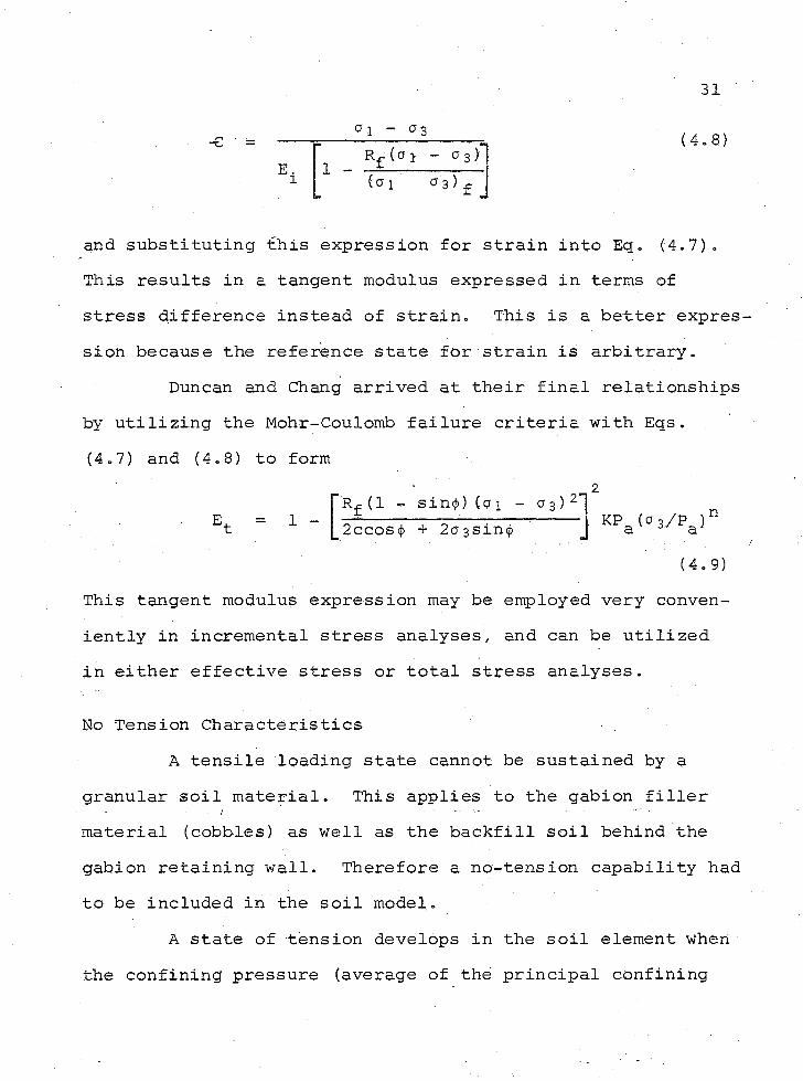
-e • (4.8)° 1 - 0 3

R£(o 1 — 0 3 ) (o 1 0 3 ) f

and substituting this expression for strain into Eg. (4.7). This results in a tangent modulus expressed in terms of stress difference instead of strain. This is a better expres sion because the reference state for strain is arbitrary.

Duncan and Chang arrived at their final relationships by utilizing the Mohr-Cou1omb failure criteria with Eqs.(4.7) and (4.8) to form

Et 1Rf (1 - sin<j>) (a 1 2 ccos<j> + 2 d 3 sin(fi

2

KPa (0 3/Pa)n

(4.9)This tangent modulus expression may be employed very conven­iently in incremental stress analyses, and can be utilized in either effective stress or total stress analyses.

No Tension Characteristics • ,A tensile loading state cannot be sustained by a

granular soil material. This applies to the gabion filler material (cobbles) as well as the backfill soil behind the gabion retaining wall. Therefore a no-tens ion capability had to be included in the soil model..

A state of tension develops in the soil element when the confining pressure (average of the principal confining

32stresses) becomes tensile. To handle this soil tension prob­lem, a no-tension provision was added to the program's soil model„

The no-tension condition was managed as follows:1 . Each soil element was checked for tension state by

calculating the average confining stress state and determining if the element is in tension.

2. If the soil element was 'found to be in tension, then a vertical stress was assigned to this element equal to the unit weight of the overburden times the height of that overburden above the soil element(av = yH). This requires that the location of the present ground surface must always be monitored throughout the construction sequence. Next the soil element's horizontal stress was given a value equal to the vertical stress times the at rest earth pressure coefficient (a — K^a^). The at rest earth pressure, coefficient (Kq = 1 - sin<|>) used in this no-tension analysis was developed by Jaky (1944).

3. Adjusting the vertical and horizontal stresses ina soil element, which is initially in tension, satis­fies two conditions. First, it gives the element a stress condition which is closer to the actual field stress condition. Second, it allows for a more rea­sonable determination of the tangent modulus for

33that soil element in the next increment of the analysis. This is due to the fact that in the Duncan and Chang constitutive model the tangent modulus is directly proportional to the confining stress.

Wire Mesh ModelTo develop a model for the wire mesh stress-strain

behavior, it was: necessary to model and analyze the wire mesh using the finite element method as described in Chap­ter 5. Previously laboratory tension tests were conducted on a gabion wire mesh by the Experimental Laboratory of the University of Bologna, Italy, and Testing Consultants, Inc., of Denver, Colorado, both clients of Maccaferri Gabions.In neither of these tension tests was the stress-strain behavior of the wire mesh determined; only the wire mesh failure stress was determined.

When considering the geometry of the hexagonal'wire mesh (Fig. 4.1) it was obvious that the wire mesh has an anisotropic material behavior. Therefore the nonlinear stress-strain behavior of the wire mesh was determined for both principal dimensions of the hexagonal wire mesh (major and minor). The nonlinear stress-strain relationship for a loading condition parallel to the major principal dimension of the hexagonal mesh is shown in Fig. 4.2, while Fig. 4.3

34

3.15 ft.-

Fig. 4.1. Typical Section of Hexagonal Triple Twisted Steel Wire Mesh Used in the Gabion Box.

02 f

t

Failure Stress

0 1 2 3 4 5 6

Strain (10 ^)

Fig. 4.2. Stress-strain Relationship for Hexagonal Wire Mesh with Loading Parallel to the Major Principal Dimen­sion of the Hexagonal.

u>U1

36

Failure Stress (Masetti, 1978)

Strain

Fig. 4.3. Stress-strain Relationship for Hexagonal Wire Mesh with Loading Parallel to the Minor Principal Dimension of the Hex­agonal .

37shows the nonlinear stress-strain relationship for a loading condition parallel to the minor principal dimension of the hexagonal mesh. Both of these curves exhibit a strain lock­ing effect.

The wire mesh nonlinear stress-strain relationships were then represented mathematically by fitting an elastic- plastic stress-strain expression to the nonlinear stress- strain curves developed from the finite element analysis.The elastic-plastic expression used for this curve fitting method was developed by Richard and Abbott (1975). The Richard and Abbott expression is a three-parameter stress- strain relationship which gives stress explicitly in terms of strain.-

c = (El S ) 1 +Ei eo

n0

-JLn

where:modulus; n

the plastic modulus;

VE - E^ ;

(4.10)

Young1s

and cthe shape parameter of the stress-strain curve;

a reference plastic stress. A detailed descriptionof the method used to fit Eq. (4.10) to the nonlinear stress- strain curve of the wire mesh (Fig. 4.2) is described in Appendix B.

To utilize Richard and Abbotts' relationship in the incremental nonlinear finite element analysis it was necessary to differentiate Eq. (4.10) with respect to strain so that

38the tangent modulus of the nonlinear stress-strain curve can be determined.

dade (El)Eie n

1 + a0«■

- (n+1)/n+ EP (4.11)

tangent modulus

No-compression CharacteristicsIn the plane strain finite element analysis of the

gabion retaining wall the' two dimensional wire mesh was modeled as a one-dimensional bar element. Since the wire mesh has no compression load carrying, capabilities, it was necessary to provide a no-compressibn provision for the bar element. The following discussion describes in general the procedure used to implement the no-compressibn provision of the bar element into the finite element program.

1. The deflections were determined for each increment in the finite element analysis.

2. New bar element lengths were determined from the deflections.

3. These new bar length were then compared with the original bar length for each bar element in. the finite element model.

4. If the new bar length was shorter than the original bar length then the bar would be in compression.All bar elements in the model which were found to

39be in compression were deactivated in the finite element analysis and therefore could contribute no stiffness to the structure and as a consequence no load could be carried in compression by these same bar elements. In addition, all bar elements which had already been deactivated in a preceding incre­ment but were found to be in a state of tension in the current increment were reactivated,

5. After deactivating the bar elements which were in compression and also zeroing the deflections for the last increment, this same increment was reanalyzed. This time no bar elements, or very few at least, would go into compression. After determining the deflections and stresses in this increment, the next increment in the analysis were initiated and the same no—compression procedure was followed.

The shortcoming of this no-compression procedure is that it is necessary to go through the simultaneous equa­tion solving subroutine twice for each increment in the analysis. This almost doubles the amount of computer time. It would be less expensive but also less accurate to go through the equation solving subroutine just once and, after the deflections and new bar lengths were determined, acti­vate or deactivate the bar elements according to whether

40they were in compression or tension. After the stresses are calculated this same procedure is initiated in the next increment.

Connecting Wire ModelThe connecting wire as described in Chapter 1 is a

3 mm single strand steel wire which is tied to the front and back of the gabion box to keep it from bulging due to the lateral force of the cobbles within the gabion box.This wire is modeled in the finite element analysis as a linear elastic bar element. Since the connecting wire can­not carry a load in compression the no-compression procedure described previously for the wire mesh bar element is also used for this bar element.

CHAPTER 5

FINITE ELEMENT MODELING

Four different cases were modeled for analysis by the finite element method. These four cases included the hexagonal wire mesh, gabion box, 1 2 ft. gabion retaining wall, and a 45 ft. gabion retaining wall.

Wire Mesh ModelingAs described in Chapter 4 the wire mesh was modeled

to determine its nonlinear stress-strain behavior. Beam elements were used to model the individual wire strands of the wire mesh.

Due to possible large deflections in the wire mesh, a geometric nonlinear analysis was used. This geometric nonlinear analysis only considered new mesh geometry in each increment of the analysis and did not continue with a series of iterations until the sum of the external and in­ternal forces in the structure approached zero or became sufficiently small (Zienkiewicz, 1971, pp. 413-417). There fore, this analysis can be considered as a first order approximation of the geometric nonlinearity of the stress- strain behavior in the hexagonal wire mesh.

41

42To determine the nonlinear stress-strain behavior

of the anisotropic hexagonal wire mesh adequately, it was necessary to consider two separate loading cases. In thefirst case the loading was applied in a direction parallelV.to the major principal dimension of the hexagonal wire mesh (Fig. 5.1), while in the second case the loading was applied in.a direction parallel to the minor principal dimension of the hexagonal wire mesh (Fig. 5^2). In both loading cases the boundary conditions can be seen in Figs. 5.1 and 5.2.

It should be noticed from Figs. 5.1 and 5.2 that the loading and boundary conditions of the finite element model simulate a laboratory test in which the wire mesh is clamped at two opposite ends and then loaded in tension. This dup­licates the loading tests conducted on a gabion wire mesh by the Experimental Laboratory of the University of Bologna, Italy and Testing Consultants Inc., of Denver, Colorado.

Single Gabion Box ModelingThe single gabion box was modeled for the purpose of

determining the load-deformation response of one gabion box under different confining stress conditions. The soil- structure interaction between the wire mesh, connecting wires, and gabion filler material (cobbles) was also analyzed

The finite element model showing both loading and boundary conditions for the gabion box is illustrated in Fig. 5.3. Due to horizontal symmetry in the gabion box, it

43

3.15 ft.

300 nodes436 elements900 degrees of freedom

Fig. 5.1. Finite Element Model of the Gabion Wire Mesh with Loading Applied Parallel to the Major Principal Dimension of the Hexagonal.

02 f

t

44

300 nodes436 elements900 degrees of freedom

Finite Element Model of the Gabion Wire Mesh with Loading Applied Parallel to the Minor Principal Dimension of the Hexagonal.

Fig. 5.2.

.02

ft

45

Wire Mes

g =Ka Cormecting Wires3 ft.

Wire Mes

1.5 ft.91 nodes 98 elements182 degrees of freedom

Fig. 5.3. Finite Element Model of a Single Gabion Box.

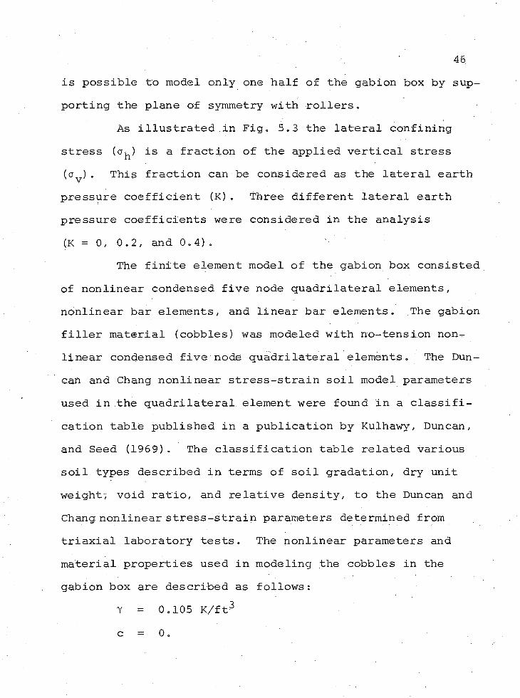
46is possible to model only one half of the gabion box by sup­porting the plane of symmetry with rollers.

As illustrated in Fig. 5.3 the lateral confining stress (c ) is a fraction of the applied vertical stress ( 0 ). This fraction can be considered as the lateral earth pressure coefficient (K). Three different lateral earth pressure coefficients were considered in the analysis (K = 0, 0.2, and 0.4) .

The finite element model of the gabion box consisted of nonlinear condensed five node quadrilateral elements, nonlinear bar elements, and linear bar elements. The gabion filler material (cobbles) was modeled with no-tension non­linear condensed five node quadrilateral elements. The Dun­can and Chang nonlinear stress-strain soil model parameters used in the quadrilateral element were found in a classifi­cation table published in a publication by Kulhawy, Duncan, and Seed (1969). The classification table related various soil types described in terms of soil gradation, dry unit weight-, void ratio, and relative density, to the Duncan and Chang nonlinear stress-strain parameters determined from triaxial laboratory tests. The nonlinear parameters and material properties used in modeling the cobbles in the gabion box are described as follows:

Y = 0.105 K/ft3

c 0 .

47<j> = 4 20

v - 0.4

K = 3 90Rg = 0.87n = 0 . 2 1

The gabion's hexagonal wire mesh was modeled as a nonlinear bar element. The nonlinear relationship shown in Eq. (4.11)

Et (E1) 1 + EieaQ

n - (n+1 )/n+ EP (4.11)

was fitted to the nonlinear stress-strain curve in Fig. 4.2 and used in the bar element to model the geometric non­linearity of a unit width of wire mesh. The nonlinear parameters of Eq. -(4.11) found when fitted with the non­linear curve in Fig. 4.2 are as follows:

EP = 3.9 x 105 K/ft2

EEi

= 5 x 104

= E - EK/ft2

1 Pn '= 1.777

= -2.6084 x 104 K/ft2

Using the above parameters in Eq. (4.11) produces the fol-2lowing relationship in K/ft : ■

48

(-3.4 x 1 0 5) (l + (13.035 e) i nn ,i\ 1« 5 6 2 7 _1-777) + 3.9 x 1 0 5

(5.1)Equation (5.1) applies only to a stress-strain con­

dition parallel to the major principal dimension of the hexagonal pattern in the wire mesh. This is the case that applies for the plane strain analysis which was utilized in the analysis of the gabion box as shown in Fig. 5.3.

The connecting wires shown in Fig. 5.3 were modeled as linear elastic bar elements with a Young's modulus equal

z: oto 4.176 x 10 K/ftz and a cross sectional area of4.09 x 10" 5 ft2.

It should also be mentioned that both the nonlinear wire mesh bar element and the linear connecting wire bar element have a no-compression provision included in their models.

Modeling 12 ft. Gabion Retaining Wall A 12 ft. gabion retaining.wall and its adjoining

backfill (Fig. 5.4) was modeled to analyze the soil-structure interaction between the gabion wall and backfill (Fig. 5.5). The gabion's wire mesh, connecting wires,, and filler mate­rial (cobbles), were all modeled with the elements, linear or nonlinear parameters, and material properties as were described in the previous section (Single Gabion Box Model­ing) .

12 ft Gabion Retaining Wall-Fig • 5.4.

V w

ir

<■

H h

2.5 D *-.5 D 2.5 D --\ \ %

193 nodes241 elements386 degrees of freedom

Fig. 5.5. Finite Element Model of a 12 ft. Gabion Retaining Wall and Surrounding Soil.

inO

A A

51The soil backfill elements were modeled with the

same no-tension nonlinear quadrilateral element used to model the cobbles.in the gabion box. ■ In some cases indivi­dual triangle elements were also used for modeling the soil backfill. Since the quadrilateral element consists of four triangle elements, the same material properties and non­linear parameters were used for both the individual triangle backfill element and the quadrilateral backfill element.

The only differences between the cobble quadrilat­eral element and the soil backfill quadrilateral element were the material properties and nonlinear parameters used to model these materials. The material properties and non­linear parameters for.the soil backfill elements are repre­sentative of a granular material and are as follows:

Y = 0.120 K/ft3

c = 0.8 K/ft2

cj) = 3 8 °V = 0 e 35K = 500R _p = 0 o 8

3" • . -

n = 0 .4

Originally, the'use of the interface element was considered for modeling the interface between the gabion wall and the surrounding soil and backfill (Sogge, 1978).It was decided that the interface element was not absolutely

52necessary since there was no distinct discontinuity between the gabion boxes and backfill soil. The backfill soil would fill the voids between the cobbles in the gabions adjacent to the backfill. This filling action results in more of a transition at the interface instead of a distinct discontinu­ity, as is found between a concrete wall and its adjoining backfill soil. Therefore the interface element was not used to model the transitional discontinuity between the gabion wall and the adjacent backfill.

The model dimensions and boundary conditions used to model a soil system of infinite extent is shown in Fig. 5.5. The lower boundary was pinned while rollers were used on both vertical side boundaries .• Studies conducted by Morgen- stern and Eisenstein (1970) showed the importance of pinning the lower boundary.

The overall dimensions of the entire model were determined after considering the previous experience of Morgenstern and Eisenstein (1970), Clough and Duncan (1971), and Sogge (1974); all three analyzed retaining walls util­izing the finite element analysis. The most significant contribution to the determination of the model's lateral dimensions came from Clough and Duncan (1971). They found that the major movements within the backfill occurred with­in a zone between the backfill and a line extending from the base of the retaining wall at an angle of 45 + <j>/2 from

53the horizontal. These findings seem to be in agreement with the 45 + 4>/2 rupture surface of the active plastic equilibrium state. The lateral dimensions of the model illustrated in Fig. 5.5 extends beyond the 45 + <j>/2 mini­mum dimension limitation.

The relative coarseness and fineness of the model's mesh, as illustrated in Fig. 5.5, was designed with respect to the expected stress gradients within the model. Areas of higher stress gradients were modeled with a finer mesh while areas of lower stress gradients were modeled with a coarser mesh.

Modeling the retaining wall as described previously does allow for the greatest, accuracy while utilizing the least number of elements. In this particular retaining wall problem there was a limitation on the coarseness of the mesh in the wall itself. This was due to the fact that the wire mesh and connecting wires of each gabion box in the retain­ing wall must be modeled. Figures 5.5 and 5.6 show how modeling the wire mesh and connecting wires in each gabion box limits the maximum size of the quadrilateral cobble elements.

The model shown in Fig. 5.5 was activated in a man­ner that would simulate sequential construction. The soil elements below the retaining wall were first activated in three consecutive layers. After the soil elements below

54

Wire mesh elementsQuadrilateral cobble element

Connecting wire elements

1 ft.

3 ft.

3 ft.

Fig. 5.6. Typical Gabion Dimensions and Element Composition.

55the wall were activated their deflections were zeroed. This was necessary since this analysis is concerned only with de­flections due to the construction of the retaining wall and backfill. The stresses in the elements below the wall were not zeroed because their in-situ stress state must be known before construction of the wall and backfill. Knowledge of these stresses was also necessary for properly modeling the nonlinear stress-strain behavior of the soil.

Next the wall construction is simulated by activating the first course of gabion boxes in the wall. In this case element activation is initiated by applying gravity loading to those elements which are being activated., Then the soil ele­ments in the backfill behind the first layer of gabions in the wall are activated to simulate the backfilling sequence behind the wall. Following this another layer of gabion boxes is constructed in the wall followed by another back­fill layer. This construction sequence is continued until the model is completely activated.

As previously described in Chapter 3,. those elements in the retaining wall and backfill, which as of that moment in the analysis have not as yet been constructed or acti­vated, are given very small stiffnesses. These small stiff­nesses in the unconstructed elements will have no influence on the deflections of the previously constructed elements,.

56while at the same time the movement or deflections of the un­constructed elements will be compatible with and follow those movements of the constructed elements. By approaching the modeling problem in this manner the original dimensions of the gabion boxes in the constructed portion of the wall will be more closely maintained resulting in a better simulation of the wall construction.

Modeling 45 ft. Gabion Retaining WallIn an attempt to verify the validity of a finite ele­

ment analysis of a gabion retaining wall, a 45 ft. gabion retaining wall (Fig. 5.7) built in the Snoqualmie Pass area east of Seattle, Washington, was modeled and analyzed using the finite element method. As previously discussed in Chap­ter 2 this wall had been monitored for deflections and stress. A comparison was attempted between the deflections and stress­es found with the finite element analysis with those obtained from the -field monitoring of the 45 ft. gabion wall.

In the Fig. 5.8, the finite element'mesh used to model the 45 ft. gabion retaining wall is shown. It can be seen in this illustration that the wall has a flat exterior face inclined towards the backfill at a slope of 8.84° or about 1:6^ (horizontal to vertical). The base of the wall also has a slope of about 1 :6 ^ (vertical to horizontal).Figure 5.7 also shows that the backfill behind the wall ex­tends 1 ^ ft. above the top of the wall while the fill in

57

45 ft. Snoqualmie Pass Gabion Retaining Wall.Fig. 5.7.

58

~7~~7 / s \ ^

33 ft.

1 2 ft.

1 gabion boxA - pin support 481 nodes 702 elements 962 degrees of freedom

Finite Element Snoqualmie Pass

Model of the 45 ft. Gabion Retaining

Wall •Fig. 5.8.

59front of the wall extends' 1 2 ft. up from the base of the wall.

In actuality the wall was constructed in the field with a gradually stepped exterior face which resulted in a slope of 1:6% (Fig, 5.7). To simplify the modeling of the wall, a flat exterior face inclined at 1:6% was used to model the wall. This is a reasonable simplification since the stepping was so gradual.

The elements used to model this wall were the same size and type as used for modeling the 12 ft. wall. The material properties and nonlinear parameters were also the same as those used for modeling the 1 2 ft. wall.

The material properties and nonlinear parameters for the gabion cobbles quadrilateral element are restated as follows:

y = 0.105 K/ ft c = 0 .<j> = 42°v = 0.4K = 390Rf = 0.87n = 0 . 2 1

The material properties and nonlinear parameters for the gabion's wire mesh bar element are restated as follows:

60E = 5 x 104 K/ft2

E = 3.9 x 105 K/ft2PE1 = -3.4 x 105 K/ft2

n = 1.777a0 = -2.6084 x 104 K/ft2

The connecting wire bar element linear material prop­erties are restated as follows:

E = 4.176 x 106 K/ft2

A — area — 4.09 x 10 ft2

Due to computer storage limitations, the backfill behind the wall and the fill in front of the wall could not be modeled. This was due to the maximum size limitations of the quadrilateral element in the retaining wall as discussed in the previous section. This size limitation fixes the num­ber of two dimensional soil elements (quadrilaterals) in the gabion retaining wall. Since the number of quadrilateral elements in the wall combined with the wire mesh and connect­ing wire bar elements were so large and utilized so much core memory, there was not enough computer storage remaining to model the backfill soil with two dimensional quadrilateral or triangle elements.

It is not possible to analyze the soil-structure interaction between the retaining wall and backfill without

61modeling the backfill. Therefore it was necessary to find a means of handling the size limitations of the core memory.

Two possible approaches were considered. Modeling the entire backfill with two dimensional elements and then utilizing a procedure called substructuring to analyze the wall and backfill was first considered. This approach was discarded since the substructure procedure would require significant modifications to the finite element program and this would be beyond the scope of this research (Richard,1978). Therefore an alternate approach was taken. The alternate approach consisted of modeling the backfill with horizontal subgrade reaction bar elements.

Terzaghi (1955) discussed in detail the concept of subgrade reaction. He defined subgrade reaction as "the pressure, P, per unit of area of the surface of contact between a loaded beam or slab and the subgrade on which it rests and on to which it transfers, the loads". He defined the coefficient of subgrade reaction, K , as "the ratio between this pressure at any given point of the surface of contact and the settlement A produced by the load application at that point". The relationship is

Ks = ~rThe value of Ks depends on the elastic properties of the

(5.2)

subgrade and on the dimensions of the area acted upon by the subgrade reaction.

62The coefficient of horizontal subgrade reaction for

a cohesionless soil was presented by Terzaghi (1955) in the following relationship:

. Kh = *h = T - (5-3)The value of the coefficient depends only on the relative density of the cohesionless soil. The relationship in Eq.. (5.3) also shows that for any depth Z below the ground sur­face, varies in a direct proportion to a ratio of the depth, Z, to the total depth, D, of the structure below the ground surface.

The concept and relationship as expressed in Eq. (5.3) was used to model the behavior of the backfill behind the.45 ft. gabion retaining wall and also the fill in front of the wall. This was accomplished by modeling the backfill soil with horizontal no-tension bar elements which would behave as springs. These bar elements were placed horizon­tally on the sides of the retaining wall (Fig. 5.8) and modeled the pressure-deformation behavior of the backfill soil in a manner as expressed in Eg. (5.3). A no-tension provision was developed for these bar elements due to the fact that soil can take very little tension and these bar elements were modeling soil behavior.

The construction sequence in the analysis of the 45 ft. wall was initiated by first activating the gravity

63loading of all the gabions in the first course or layer of the wall. After analyzing the first sequence in the construc­tion of the wall, the no-tension bar elements representing the solid backfill behind and in front of the first layer of the wall were activated. As these horizontal no-tension bar elements were activated, their end furthest from the retain­ing wall was supported both horizontally and vertically. Fol­lowing this the construction sequence is continued with more layers of gabions being activated followed by more horizontal no-tension bar elements until the construction sequence is -completed for the entire wall.

As the wall was constructed and each new layer of horizontal no-tension bar elements activated, it was neces­sary to impose an initial horizontal displacement at the supported end of these horizontal, no-tension bar elements. Actually all of the previously activated no-tension bar ele­ments would require additional imposed horizontal displace­ments for each increase in the height of the backfill. For each increase in the height of the backfill the imposed horizontal displacements in all of the previously and newly activated no-tension bar elements can be determined by the following relationship.

A JL _ K y Z _ K y H Kh (Z/H) Ji,h • Ah (5.4)

64Y = 0.12 K/ft^ = unit weight of backfill.H = the present height of the backfill at that

moment in the construction sequence. For newly activated no-tens ion bar elements the total existing height of backfill is used, while for previously activated no—tension bar elements only the height of the last increment or layer of backfill is used.

Z = distance of no-tension bar element below thepresent backfill ground surface.

3= 20 K/ft = a subgrade constant which is depen­dent on the.. relative density of the soil (Terzaghi, 1955, p. 319).

K = 0.5 = lateral earth pressure coefficient whichis used to approximate the lateral pressure at any point on the side of the wall due to each additional increase in backfill height.

Besides imposing displacements in the no-tension bar elements to simulate the horizontal subgrade reaction between the retaining wall and backfill, gravity loading was applied to the horizontally stepped surfaces on the back face of the retaining wall (Fig. 5.8). This loading requirement was neces sary due to the weight of the overlying backfill soil.

65The material properties of the horizontal no-tension

bar element are as follows:2A = 1 ft = cross sectional area of the soil backfill

that the bar element represents.& = 1 ft = the unit length of the activated bar ele­ment. E = the modulus of the soil,

The relationship for E

E = Kh = -r *hcan be developed in the following manner:

PE “ A/£ *

Now combining Eq. (5.3) with Eg. (5.6) results inkt

E = h A A/£

and

Kh £but for £ = 1 ft (unity), then

E = Kh = IT ^h »

(5.5)

(5.6)

(5.7)

(5.8)

(5.9)

Equation (5.9) shows that the modulus of the horizontal no­te ns ion bar element will increase with depth from the top of the backfill surface. This concept is compatible with Janbu's (1963) relationship as expressed in Eq. (4.4) which relates

66the initial tangent modulus with the confining pressure in the soil. Since it is known that confining pressure increases with depth, it is therefore recognized that Eqs. (4.4) and(5 .9 ) are common in that both of these equations relate a soil modulus to a depth below the ground surface.

CHAPTER 6

PRESENTATION AND DISCUSSION OF FINITE ELEMENT ANALYSIS RESULTS

In the following presentation the results of the finite element analyses of the gabion wire mesh» single gabion box, 12 ft*' gabion retaining wall, and 45 ft. gabion retaining wall will be discussed. In addition a comparison will be made between a conventional stability analysis of the 1 2 ft. gabion retaining wall versus a stability analysis of the same wall utilizing the results of the finite element analysis.

Wire MeshDue to the anisotropic stress-strain behavior of the

gabion's hexagonal wire mesh, two separate loading conditions of the wire mesh were analyzed as described in Chapters 4 and 5 and illustrated in Figs. 5.1 and 5.2. Both of these analyses produced material properties and nonlinear param­eters for the wire mesh relative to the major or minor prin­cipal dimensions in the hexagon of the wire mesh. Figures 4.2 and 4.3 indicate the geometric nonlinear stress-strain behavior of the wire mesh under both loading conditions. As previously mentioned in Chapter 4, the nonlinear stress- strain behavior for both loading conditions in the wire mesh exhibited a strain locking condition.

67

68The strain locking result was expected due to the

hexagonal geometric pattern of the wire mesh. It can be observed in Pigs. 5.1 and 5.2 that for both loading conditions the initial hexagon geometric pattern has many steel wires at an angle of 45, degrees with respect to the direction of load­ing. As the load is applied and subsequently increased, strains begin developing in the wire mesh, and the wires which were originally at an angle of 45 degrees with respect to the direction of loading are now at an angle less than 45 degrees. The reorientation of these wires towards an orien­tation which approaches the direction of loading can occur initially without significantly increasing the strains in each wire element, but as these wire elements become more oriented parallel to each other there is less allowance for displacements without strain and therefore any further dis­placements will be resisted by a stiffer structure resulting in a strain locking condition.

As previously described in Chapter 4 the non-linear stress-strain behavior of the wire mesh was represented mathe­matically by fitting an elastic-plastic stress-strain expres­sion, developed by Richard and Abbott (1975), to the nonlinear stress-strain curves of Figs. 4.2 and 4.3. A detailed de­scription of the development of the wire mesh's elastic- plastic nonlinear stress-strain model [Eq. (4.10)] is given in Appendix B.

69Due to the hexagonal geometric pattern of the gabion

wire mesh, the Poisson's ratio of the wire mesh should vary with respect to strain.. Because of the geometric anisotropic properties in the wire mesh this variation will be different for both loading conditions illustrated in Figs. 5.1 and 5.2.

The nonlinear variation of Poisson's ratio with re­spect to strain is illustrated in Figs. 6.1 and 6.2. Figure 6 . 1 is for a condition in which strain is in a direction parallel to the major principal dimension in the hexagonal wire mesh while Fig. 6.2 is for the condition in whi&h strain is parallel to the minor principal dimension in the hexagonal wire mesh. It can be seen in both cases that the Poisson's ratio increases with strain.

The determination of the variation of Poisson's ratio with strain was of no consequence in the finite element analysis utilized in this research to study the behavior of the gabion box and gabion retaining wall. The variation of Poisson's ratio with strain will be of more importance during the development of constitutive equations for the gabion box.

Gabion BoxAs previously described in Chapter 5 and illustrated

in Fig. 5.3 the gabion box was analyzed to study the load- deformation behavior of a single gabion box under different confining pressures. The Results of these analyses are shown in Fig. 6.3.

70

Fig. 6.1. Nonlinear Variation of Poisson's Ratio with Respect to Strain in a Direction Parallel to the Major Principal Dimen­sion in the Hexagonal Wire Mesh.

71

Strain e

Nonlinear Variation of Poisson's Ratio with Respect to Strain in a Direction Parallel to the Minor Principal Dimen­sion in the Hexagonal Wire Mesh.

Fig. 6.2.

72

CN-P4-)XXmtn(UM-PtZ)i—IrdU•H4-)M>

K=. 4 K=. 2

Vertical Strain

Vertical Stress Applied to Top of Gabion Box Versus Vertical Strain in Gabion Box.

Fig. 6.3.

73From Fig. 6.3 it can be seen that for all three con­

fining cases (K = 0, 0.2, 0.4) there was initially a'stress-. strain curve similar to what may be expected from the gabion filler material (cobbles). Then as the stress and strain, increased the curve exhibited more of a strain locking beha­vior similar to the behavior observed in the wire mesh.

This is basically the stress-strain behavior which was expected. As the load was first applied to the gabion box the filler material (Fig. 5.6) initially carried all the load. During this period of initial loading, vertical deformation occurred while accompanied by an outward lateral deformation of the gabion box. As the lateral deformation increased the stresses in the horizontal wire mesh and connecting wires (Fig. 5.6) began to increase resulting in a greater lateral confinement (confining pressure) on the gabion filler mate­rial . As the stresses in the horizontal wire mesh and con­necting wires continued to increase, additional lateral confinement was developed on the gabion filler material with a resulting overall increased stiffness for the entire gabion box as observed in Fig. 6,3 for all three initial confinement conditions. It can also be seen in Fig. 6.3 that as the lateral earth pressure loading coefficient (K) was decreased, the gabion box required a greater amount of vertical strain to develop an adequate confining pressure in the gabion box

74filler material to increase the stiffness of the entire gabion box resulting in the strain locking behavior.

The fact that any increase in lateral confining pres­sure in the gabion filler material resulted in a greater stiffness in the entire gabion box, can be explained by an examination of the Duncan and Chang (1970) soil model [Eq.(4.9)] which was used to model the gabion filler material.In this model the tangent modulus of the gabion filler mate­rial is proportional to the confining pressure on the filler . material. Since the stiffness of the gabion filler material increases with any increase in its tangent modulus, it can therefore be realized that any increase in the gabion filler material's confining pressure will result in an increased stiffness for the entire gabion box. This increase is par­tially balanced by the decrease in the tangent modulus with strain.

The variation of connecting wire stress in the gabion box with increased applied vertical stress is illustrated in Fig. 6.4. As expected, the connecting wire stress is great­est for the K = 0 applied confining condition. For this con­fining condition there is the greatest lateral deformation in the gabion box.

Figure 6.4 also illustrates the various levels of stress at which failure can occur in the connecting wires.It should be added here that even if failure occurs in the

75

CM4->M-l\%10CO0)u-Mini—irdu•H+J>

K=. 4 K=. 2

Connecting Wire Stress (10^ K/ft^)□ - failure stress for carbon steel connecting

wire = 10080 K/ft ; from Annual Book of ASTM Standards, 1979, p . 685.A- failure stress for high carbon steel connecting wire = 17568 K/ft ; from Byars and Snyder,(1975, p. 470)

Fig. 6.4. Vertical Stress Applied to Top of Gabion Box Versus Connecting Wire Stress in Gabion Box.

76connecting wires it will not be very significant on the over­all stability of a gabion structure such as a retaining wall. If the connecting wires fail, the gabion box will bulge more „ in the middle and a small additional stress will be trans­ferred to the wire mesh. The main function of the connecting wires is to prevent the exposed faces of the gabion box from bulging outward. A bulge should not produce any stability problems but by preventing any bulging of the exposed faces will provide a more aesthetic structure.

The maximum stress developed in the wire mesh wasO2207 K/ft which is much less than the wire mesh failure

o 2stress of 5552 K/ft . The failure stress of 5552 K/ft was found in wire mesh tension tests conducted at the Experimental Laboratory of the University of Bologna, Italy (Masetti, 1978)

12 ft. Gabion Retaining Wall The 12 ft. gabion retaining wall and backfill illus­

trated in Fig. 5.4 and modeled in Fig. 5.5 was analyzed to determine the soil-structure interaction between the retain­ing wall and backfill and also the soil-structure interaction within the gabion box itself. Various aspects of the wall behavior were analyzed, such as wall deflections and stress distributions throughout the wall and backfill.

The horizontal deflections of the retaining wall exterior face are shown in Fig. 6.5. Two results are plotted

77

12 ft.

Wall Deflection Away from Backfill (ft.)□ - displacement relative to the original designed

spatial location of wall.A - displacement relative to the moment of construction.

Fig. 6.5. Horizontal Deflections for the Exterior Face of the 12 ft. Retaining Wall.

78on this graph, one curve represents the displacement of the wall relative to its original designed spatial location and orientation, while the other curve represents the actual dis­placements at different elevations on the wall which occurred during and after construction of that level or elevation of wall.

Both curves in Fig. 6.5 show that the exterior face of the wall is moving in a direction away from the backfill. When considering the displacement of the wall relative to its original designed location it can be seen that the wall move­ment was mostly translational with a slight amount of rota­tion about the base of the wall. It can also be seen from Fig. 6.5 that the deflections of the wall relative to its original designed spatial location was normally greater than the deflections incurred at various elevations of the wall after construction of these corresponding elevations. This was expected since movements and tilting of previously con­structed layers of gabions will affect the location of gabion layers which have as yet hot been constructed in the wall.

The horizontal deflections of the back face of the 12 ft. retaining wall are illustrated in Fig. 6.6. The back face of the wall also shows a movement away from the backfill which results in an active loading condition on the back of the wall. The same mode of wall movement is seen in Fig. 6.6 as was seen in Fig. 6.5 with translational wall movement

79

12 ft

Wall Deflection Away from Backfill (ft.)□ - displacement relative to the original designed

spatial location of wall, displacement relative to the moment of construction.

Fig. 6.6. Horizontal Deflections for the Back Face of the 12 ft. Retaining Wall.

80being most significant combined with a small amount of tilting

a 'along the base of the wall. As expected, once again the de­flections of the wall relative to its original designed spa­tial location were normally greater than the deflections incurred at various elevations of the wall after construction of these corresponding elevations.

It was also recognized from Figs. 6.5 and 6.6 that the exterior face of the retaining wall had a slightly greater movement away from the backfill as compared with the movement of the back face of the wall. This was the result of an out­ward bulging of the gabion wall itself due to gravity loading of the gabions themselves. Since the exterior face of the retaining wall was exposed and not confined, its outward deflection was a combination of a small amount of wall bulging plus a much greater amount of translational wall movement.

A contour map illustrating the vertical stresses developed in the gabion retaining wall, backfill, and under­lying soil is shown in Fig. 6.7. A simular contour map show­ing the horizontal stresses is illustrated in Fig. 6.8. Due to the uniformity and flatness of the stress contours near the outer lateral boundaries as seen in both figures, it can be concluded that the lateral dimensions of the model were of adequate extent to negate any boundary influence.

Fig. 6.7. Vertical Stress Contour Map of 12 ft. Gabion Retaining Wall and Backfill.

00

Fig. 6.8. Horizontal Stress Contour Map of 12 ft. Gabion Retaining Wall and Backfill. ooNJ

83When examining the wall in Figs. 6.7 and 6.8 it can

be seen that both the vertical and horizontal stresses ini­tially increase when moving from the exposed exterior face of the wall towards the back of the wall. The stresses (especially horizontal stresses) near the exposed exterior face will always be smaller due to the lack of confinement. Between the middle and back of the wall the stresses seem to reach a peak and then begin to decrease as the back of the wall is approached.

In the backfill behind the wall the stresses decrease sharply followed by a gradual increase to an in-situ stress state at a point located halfway between the wall and the lateral boundary. The sudden sharp dip in the stress con­tours behind the wall can be attributed to'the outward move­ment of the wall resulting in an active stress condition in the backfill soil as illustrated in Fig. 6.9.

Figure 6.9 shows the horizontal pressure on the back face of the wall to be less than the in—situ triangular earth pressure distribution. This horizontal pressure distribution was not triangular as would be in the case when a rigid wall rotates outward along its base nor was it parabolic as would be expected from an outward translational movement of a rigid wall along its base as described by Terzaghi (1941), Tschebotarioff (1951, 1962).

84

12 ft. Retaining Wall

In-situ Earth Pressure Distribution (K =l-sin<f>)Active Earth Pressure Distribution (Coulombs)

Horizontal Pressure on Back Face of Wall (K/ft )

Fig. 6.9. Horizontal Pressure on Back Face of 12 ft. Retaining Wall Versus Wall Elevation.

85Due to the outward rotation of the 12 ft. gabion wall

a triangular horizontal pressure distribution would be'ex-' pected on the back of the wall, but Fig. 6.9 shows that the resulting, pressure distribution was not exactly triangular.Two possible explanations can be given for this difference in horizontal pressure distribution. It should first be pointed out that Coulomb's triangular pressure distribution was originally developed for a rigid wall rotation about the toe while in this case the gabion wall is a more flexible structure with bending included in its rotation. Secondly, shorter rigid walls are often constructed entirely before the backfilling is initiated, while the gabion wall is constructed in a sequence With backfilling following each course of gabions. This difference in construction sequences can affect the horizontal pressure distribution on the back of the wall.

From Fig. 6.7 it can be seen that the vertical stresses in the backfill immediately behind the wall are re­duced and these stresses are redistributed into the gabion wall. This redistribution of stress can be seen in the peak­ing of vertical stresses in the wall itself. This is not an arching action but a load transfer through vertical shearing brought about by the relative differential movements between the gabion wall and backfill. The wall is moving outward while the backfill is moving outward and downward.

86Tschebotarioff (1951, 1973) discussed the difference

between a true arching and the transfer of pressures by shear. He explains that the terms "arching" and "transfer of pres­sures by shear stresses" are not synonymous. He suggests that arching does involve some transfer of pressures by shear, but pressures can be transferred by shear without any arching being involved. Tschebotarioff feels that a stable true arch can develop only if the walls forming an abutment for the arch are unyielding and if the individual soil grains are hard and nondeformable; thus it cannot develop in plastic clays. If these conditions for a true arch exist then it would be expected that the lateral earth pressure coeffi­cient, K, would be locally greater than one, which would reflect the progressive wedging and jamming of individual sand grains, i.e ., a process which is the reverse of sliding.

It can be seen in Pigs. 6.7 and 6 . 8 that no unyield­ing abutment conditions exist and in no area of the wall and backfill is K >1, therefore it can be concluded that no arching condition developed in the backfill. This is a reasonable conclusion since arching is more commonly found in active conditions where wall movements are translational or rotational about the top of the wall (Tschebotarioff,1951).

The location of two cross sections (A and B) taken through the 12 ft. gabion wall are shown in Pig. 6.10.

A

1 2 ft.

G a b i o n ^

Fi9- 6.10.

88Through both cross sections the connecting wire stress versus wall elevation is plotted in Fig. 6.11 while the wire mesh stress versus wall elevation is plotted in Fig. 6.12.

As expected the connecting wire stress is greatest in the gabions near the bottom of the wall (Fig. 6.11). The gabions near the bottom of the wall have higher overburden pressures and therefore exhibit greater bulging resulting in increased connecting wire stress. The decrease in connect­ing wire stress at the 1 ft. wall elevation can be explained by the restrainment of the lowest course of gabions by the soil below these gabions. It should also be noticed in Fig, 6 . 1 1 that the stresses in the connecting wires are greatest near the exposed face of the gabion retaining wall. This is a reasonable result since the gabions on the exposed face will exhibit the greatest amount of bulging and therefore higher connecting wire stresses.

The results of the wire mesh stress versus wall ele­vation as illustrated in Fig, 6.12 are comparable with the results found for the connecting wire stress in Fig. 6.11.The previous section's description of the results and be­havior of .the connecting wires are just as valid for describing the results and behavior of the wire mesh. There­fore it will not be necessary to redescribe the behavior of the wire mesh with respect to its results.

89

6.11. Connecting Wire Stress Versus Wall Elevation.Fig.

90

O Section AA Section B

Wire Mesh Stress (K/ftz)

Fig. 6.12. Wire Mesh Stress Versus Wall Elevation.

• 91Finite Element Versus Conventional Stability Analysis

An attempt is made here to compare the finite element stability analysis of the 1 2 ft. gabion retaining wall with the conventional stability analysis of this same wall. The conventional stability analysis of the 1 2 ft. gabion retain­ing wall was previously described in Chapter 2 and is present­ed in Appendix A. The finite element stability analysis of this same wall is presented in Appendix C. The results of both analyses are summarized in Table 6.1.

From Table 6.1 it can be seen that there seems to be a significant difference in the factors of safety between the two methods of analysis. The factors of safety determined in the finite element stability analysis are less than those determined from the conventional stability analysis. One exception to this is the factor of safety of the wall in bearing capacity stability with respect to shear strength.In this case the conventional analysis had the higher factor of safety. Actually the factor of safety of bearing capacity with respect to shear strength is probably meaningless in this problem since the footing is so wide and therefore allowable settlement will probably be the limiting condition for bearing capacity stability.

Table 6.1. Factors of Safety (F.S.) for Conventional and Finite Element Stability Analysis of the 12 ft. Gabion Retaining Wall.

Factor of SafetyOverturning about toe of wallSliding along the base of the wallBearing capacity with respect to shear strength

Conventional Analysis ________of Wall______

7.8

17

14

Finite Element Analysis __________ of wall ____

3.7

11

21

9 345 ft. Gabion Retaining Wall

The results of the finite element analysis of the 45 ft. gabion wall illustrated in Fig. 5.8 were very dis­couraging and are no doubt unreliable. There seemed to be no continuity or uniformity in the stress distribution throughout the entire wall. Because of the nonuniformity of stress distribution throughout the wall it was impossible to plot stress contours.

The nonunifofmity of the stress distribution can no doubt be attributed to the attempt to model the backfill with horizontal subgrade reaction bars. The analysis of the prob­lem was complicated by the sequential construction require­ments of the wall and backfill. Since horizontal subgrade reaction bars were used to model the backfill, the successive backfilling operations had to be simulated in the horizontal subgrade reaction bars by imposing successive horizontal dis­placements in these bars to account for each backfilling sequence.

It was not possible to establish exactly what pro­duced the nonuniformity of the stress distribution in the wall but it is the writer's opinion that the inadequacy of the analysis can be attributed to the attempt to model the sequential backfilling by imposing successive displacements on the horizontal subgrade reaction bars and at the same time altering the stiffness of these elements at each sequence of backfilling.

94Even though the stress results are considered invalid,

the wall's displacement results illustrated in Fig. 6.13 seem plausible. These displacements should still be questioned but at least they show a wall movement which is reasonable.An active condition was developed by the displacements shown in Fig. 6.13.

95

o •

• o

• o• o

• O

Deflection toward | Deflection the backfill (ft) ' away from

backfill(ft)

Q - displacement relative to the original designed spatial location of wall.

0 - displacement relative to the moment of construction.

Fig. 6.13. Horizontal Deflections for the Exterior Face of the 45 ft. Gabion Retaining Wall.

DEVELOPMENT OF CONSTITUTIVE 'EQUATIONS FOR A GABION BOX

A set of constitutive equations for a single gabion box will be developed in this chapter. The detailed develop­ment of these equations is given in Appendix D.

The development of these equations will allow for the future development of one quadrilateral finite element repre­senting a single gabion box. The utilization of this element will have a significant effect on decreasing the number of elements and also the total number of degrees of freedom in the model. This will result in decreased core memory require­ments and also probably smaller computer costs.

The development of the constitutive equations for the gabion box paralleled the development of constitutive equa­tions for reinforced earth as formulated by Romstad, Herr­mann, and Shen (1976). The gabion box was first characterized as a composite material. Next a unit cell concept was util­ized to relate the behavior of the gabion composite with the material properties and geometric arrangement of the indivi­dual components within the gabion composite (cobbles, wire mesh, and connecting wires).

CHAPTER 7

96

97For a structure that has a regular reinforcing pattern

such as the gabion retaining wall exhibits, it is possible to isolate a small unit of this structure (gabion box) which completely exhibits the composite characteristics of the structure and gabion box; this fundamental building block is called the unit cell or representative volume. The following description by Romstad et al. (1976, p. 457) more clearly de­fines the unit cells application to composite materials.

The average values of the stresses distributed over the cell faces are equal to the stresses in the equivalent composite material, and the average values of strains for the cell are those of the composite.Thus, the average response of the unit cell to a homogeneous state of composite stress or strain is the same as the composite response of the material. There­fore, the desired composite properties may be calcu­lated from a detailed consideration of the behavior of the unit cell. These composite properties may then be used in a structural analysis of the complete struc­ture. Such an analysis yields the composite stress and strain throughout the structure; once the compo­site stress stafe is determined at a particular point in the structure, the corresponding constituent stress state may be determined by returning to the analysis of the unit cell.

A diagram showing the gabion box unit cell is illus­trated in Appendix D, Fig. D.l. The stress-strain matrix Eq. (D.2) is also shown in Appendix D. The constitutive equations for the gabion box are developed by solving for the c^j parameters in the matrix. It should be noted thatthe stress (a ■) t strain (e.), and matrix parameters (c. .)J J 3-J

98are all incremental values resulting from the incremental application of loading on the structure or unit cell. This incremental analysis is necessary to adequately consider the nonlinear behavior of the unit cells individual components.

CHAPTER 8

CONCLUSIONS AND RECOMMENDATIONS

ConclusionsThe conclusions pertaining to the wire mesh, gabion

box, and gabion retaining walls will all be discussed sep­arately. The following conclusions were developed from the results of the analysis of the wire mesh:

1. The gabion's hexagonal wire mesh exhibited aniso­tropic material properties due to the hexagonal geometric pattern in the wire mesh.

2. Because of this geometric pattern in the wire mesh, a geometric nonlinearity was produced in the stress- strain behavior of the wire mesh.

3. It is also considered that the strain locking exhibited by the stress-strain curve of the wire mesh was also a result of the hexagonal geometric pattern in the wire mesh.

4. The nonlinear increase in Poisson's ratio with strain for the wire mesh can be once again attributed tothe hexagonal geometric pattern of the wire mesh and the resulting strain locking effect which is devel­oped.

99

The following conclusions were developed from the results of the analysis of the single gabion box:

1. The stiffness of the gabion box increased as the applied confinement loading was increased. This was expected since the stiffness of the soil as repre­sented in the Duncan and Chang soil model is propor­tional to the confining stress in the soil.

2. The nonlinear stress-strain curve of the gabion box initially exhibited a strain hardening behavior as might be expected from a cohesionless soil, but sud­denly the gabion box stiffened and a strain locking behavior developed. The strain locking behavior can be attributed to the lateral deformation of the gabion box which allowed for the stiffening of the gabion box through the contribution of the wire mesh and connecting wires. As lateral deformation in­creased the wire mesh and connecting wires developed greater stresses which in turn produced more confine­ment in the cobbles resulting in a stiffen gabion box.

3. The failure of the connecting wires in the gabion box were directly related to the amount of applied confinement loading on the gabion box. This means that as the applied confinement loading was increased, the vertical loading on the top of the gabion could also be increased without failing the connecting

101wires in the gabion box. The additional confinement allows for less lateral deformation in the gabion box and therefore less stress build up in the connecting wires. The applied confinement loading affects the wire mesh in the same manner as was previously de­scribed for the connecting wire.

The following conclusions were developed from the results of the finite element analysis of the gabion retain­ing walls:

1. The wall movements for both the 12 ft. and 45 ft. gabion retaining walls resulted in an active stress condition in the soil immediately behind the walls.The 12 ft. wall had a translational movement plus a small outward rotational movement while the 45 ft. wall also had a translational movement but its wall rotation was opposite to that of the 1 2 ft. wall.

2. The horizontal pressure distribution oh the back face of the 1 2 ft. gabion wall also showed an active stress condition.

3. Both the 12 and 45 ft. gabion Walls exhibited outwardbulging. •

4. The 12 ft. gabion wall had a reduction and redistribu­tion in the vertical and horizontal stresses in the soil immediately behind the wall. This stress reduc­tion was attributed to a load transfer through

102vertical shearing. Arching was not the mechanism producing the stress reduction and redistribution.

5. The connecting wire stresses and wire mesh stresses were greatest in the gabions near the bottom of the wall and closest to the exterior face of the gabion wall.

6 . When comparing the results of the conventional stabil ity analysis of the wall with the finite element stability analysis of the wall it was found that the finite element analysis in general gave lower factors of safety and therefore was more conservative.

7. The invalid stress results from the 45 ft. gabion retaining wall were attributed to the attempt to model the backfilling sequence with a sequential activation of horizontal subgrade reaction bars.

Design ApplicationsThe finite element analysis can provide a valuable

tool in the design, of gabion retaining walls. The conven­tional stability analysis which is most commonly used today for the design of gabion retaining walls has many limitations brought on by the assumptions made in this analysis. The first assumption made in the conventional analysis is to design the gabion wall as a rigid mass gravity structure with an active triangular Coulomb earth pressure distribution acting on the back of the wall. The gabion wall is not

103actually rigid and the earth pressure distribution may not necessarily be triangular. The wire mesh and connecting wires are not considered in the conventional analysis, their effect is only considered as an additional safety factor.

The following description will provide an outline of the finite element design applications in the gabion retain­ing wall which are not possible when utilizing the conventional method of analysis and design:

1. The stress distribution can be determined throughout the wall and backfill. The stresses in the component parts of the gabion such as the wire mesh and connect­ing wires can also be determined.

2. By knowing the stress distribution in the backfill, the earth pressure on the back of the wall is known.

3. The maximum wall height capable of producing a fail­ure in the wire mesh or connecting wire can be deter­mined,

4. Wall movements can be determined. This determination is important for construction projects where it is necessary to know the final spatial location and orientation of the wall after construction.

5. The optimum wall inclination which will produce the desired wall movements and allowable, wall stresses can also be determined. Too much inclination could possibly produce a backward rotation of the wall

104resulting in a passive stress state in the backfill near the top of the wall.

6 . The effect of sequential wall construction and back­filling can be studied with the finite element analysis.

7. Various possible wall shapes and configurations plus gabion box distributions can be more adequately studied with the finite element analysis.

Recommendations for Further Research Very little research has been done with gabions.

Previously many of the gabion uses,- capabilities, limitations, and designs were based on past experience through trial and error. The finite element method provides a means of more adequately analyzing the gabion box and gabion structures.The following summary outlines areas of possible further re­search with gabions:

1. Develop stress-strain curves for the wire mesh from laboratory testing and compare with those developed from a finite element analysis of the wire mesh as describe d i n Chapter 5.Determine the stress-strain behavior of a gabion box from laboratory testing and compare with the finite element analysis of the gabion box as described in Chapter 5.

2.

3. Compare the stability of a vertical stepped exterior­faced gabion retaining wall as shown in Fig. 1.6 versus the inclined flat exterior-faced gabion retain­ing wall as illustrated in Fig. 1.7.

4. Determine the optimum angle of inclination of the inclined gabion retaining wall illustrated in Fig.1.7 with respect to the wall's stability and the stress distribution throughout the wall and backfill.

5. Analyze the 12 ft. gabion retaining wall illustrated in Fig. 5.5 with interface elements included along the back and base of the wall. Compare these results with those presented in Chapter 5.

6 . The constitutive equations developed in Chapter 7 could be used to develop a single four node quadri­lateral finite element which would represent and model a gabion box. The use of this element in modeling a gabion retaining wall could then be compared tizith the method described in Chapter 5 to model the retaining wall illustrated in Fig. 5.5.

105

(

APPENDIX A

CONVENTIONAL STABILITY ANALYSIS OF A 12 FT. GABION RETAINING WALL

The gabion retaining wall is normally analyzed as a rigid mass gravity structure in the conventional stability analysis (Maccaferri Gabions Publications, 197 4 and 1977) . Figure A.l illustrates a 12 ft. gabion retaining wall and shows the internal and external forces which are applicable to a conventional stability analysis of this Wall. As with most conventional stability analyses of mass gravity walls, three possible modes of failure are analyzed; overturning about toe, sliding along the base, and a bearing capacity failure of the foundation. The conventional analysis proceeds as follows:

1. Determine the active earth pressure (P_) acting on the back of the gabion wall utilizing Coulombs wedge method analysis.P, = 1/2 K yH 2cL clK = lateral active earth pressure coefficient sY - unit weight of backfill = .12 K/ft2

H = wall height = 1 2 ft.

106

107

6 FT

/ / / / \ \ \ V

12 FT

6.4FT-

3.4 FT

I I I \ \ \ \

Fig. A.1. 12 ft. Gabion Retaining Wall Analyzed as a Mass Gravity Structure.

10 8

esc 8 sin (8 -4 )________ ______V— T r )

<i> = angle of internal friction for backfillsoil = 38°

6 = angle of wall friction = .94> = 34.2°8 =. angle of top surface of backfill with respect

to the horizontal = 0

0 = angle between back of wall and the horizontal= 84.29°

esc ( 84.29) sin ( 84.29-38)____ ________ 'j/sin (84.29+34.2) + •/ S'1° 8"2>

K = 0.1815aPa (0.5)(0.1815)(0.12 K/ft3) (12 ft)2 (1P 1.568 KaPv = (1.568 K) sin 28.49° = 0.8813 Kph (1.568 K) cos 28.49° = 1.297 K

2. Analyze overturning stability of wall.a. Determine the gravity weight (W) of the wall.

Area of wall = 58.5 ft^Unit-weight of cobbles in the gabions = 0.105 K/ft6

W = (0.105 K/’ft3) (58.5 ft2)

./

W = 6 e143 K

109b. Determine the horizontal center of gravity of

the wall from Fig* A.l. -X = 3.115 ft.

c. Determine the surcharge loads on the horizontal steps of the gabion wall's back face.S1 = (0.12 K/ft3)(6.525 ft)(1.5 ft)(1 ft) =

1.175 K. S2 = (0.12 K/ft3 )(3.375 ft)(1.5 ft)(1 ft) =

0.6075 Kd. Determine the horizontal distance from the toe of

the wall at which the resultant of W, , and S2

act._ wx + s1 x1 + s2 x2 wx + s 1 x1 + s2 x2

t w + + S2

- _■ (6.143K) (3.115 ft) + (1.175K) (5.85 ft) + (0.6075K) (4.65ft)r 6.143K + 1.175K"+ 0.6075K

Wr = 7.926 KX = 3.638 ft.' r

e. Factor of safety must be greater than or equal to 1.5.

r _ r _L_ „ . ~Mr summation of resisting momentsFactor of Safe y - . . - - sumination of overturning moments

_ WrXr + Pv ( 6 ‘ 4 £t) = (7.926KV (3 - 63 8 ft V +' (. 8813K) (6.4ft) . S'b" Ph (3.4 ft) (1.297K)(3.4 ft)

F.S. = 7.82 > 1.5

- ‘i

1103„ Analyze sliding stability of wall.

a. Determine the normal (N) and tangential (T) load components on the base.

N = (Wr+Pv)cos(5.71°) + Phsin(5.710)N = (7.926 K + .8813 K)cos(5.71*) + 1.297 K sin(5.71°)

. N % 8 . 89 3 KT = Ph cos(5.71°) - (Wr+Pv)sin(5.71°) -T =1.297 K cos(5.71°) - (7.926 K + .8813 K)sin(5.71°)T = .4143 K

b. Factor of safety must be greater than or equal to 1.5. Along the base of the gabion wall the wall friction angle is assumed to be equal to the soil's angle of internal friction.

r summation of shear resisting forces ~ summation of tangential driving forces

_ N tan _ (8.893 K)tan(38°)T .4143 KF.S. =■ 16.77 > 1.5

4. Analyze for shear strength bearing capacity stability of the wall.a. Determine from Fig. A.1 if the resultant of the

forces passes through the base within its middle third. If the resultant passes through the middle third of the base then it can be assumed that the foundation loading is distributed linearly over

F.S,IF

the entire base width.

Illb. Determine the eccentricity (e) of the resultant

force with respect to the middle of the base.

B = gabion wall base width = 6 ft. e = u - B/2 = u - 6 ft/2

Mr~Mo _ (7.926K)(3.638ft)+(.8813K)(6.4ft)-(1.297K)(3.4ft) u “ N 8.893 K

u = 3.381 ft.e = 3.381 ft - 3 ft = .381 ft.

The eccentricity shows that the resultant of the forces intersects the base within its middle third.

c. Determine the linear pressure distribution alongthe base. The minimum stress acts at thetoe of the base while the maximum stress (a.)iacts at the heel of the base.

aa12>

al

°1

N P, + € eB B

8.893 K \ (6 ) (.381 ft)'6 ft i 6 ft

2.047 K/fV

a 2

a 2

8.893 K ‘ (6)(.381 ft)6 ft 1 6 ft

= .9175 K/ft1 2

112d. Calculate factor of safety

qult = C N =q + y 2 ny(ic == cohesion = . 8 K/ft^

NCq 4.9 (for inclined footing)

\ q •70 (for inclined footing)

qult. == ( . 8 K/ft2)(4.9) + (.12 K/ft

qult 29.12 K/ft2

qmax = = 2.047 K/ft2 •.

F.S. r= qult 29.12 K/ft2

%nax 2.047 K/ft2

(70)

F.S. 14.23

APPENDIX B

WIRE MESH NONLINEAR STRESS-STRAIN ELASTIC-PLASTIC FITTING METHOD

Nonlinear Stress-strain Fitting .Method for Loading Parallel to Major Principal

Dimension of Wire MeshA hypothetical curve of Richard and Abbott1s (1975)

nonlinear elastic-plastic stress-strain relationship

an

= (E^e) 1 + El£ao

1n

+ E e P (4,10)

is illustrated in Fig, B.l, .Referring to Fig. B.1, E^ = theplastic modulus; E, = E - E ; n = the shape parameter of thePstress-strain curve? and a - a. reference plastic stress.

Richard and Abbott (1975) explain that the shape parameter n may be obtained by forcing the analytical expres sion [Eq.(4.10)] through two points on the stress-strain curve (ea/°a) and where, for convenience, = 2 eaThe resulting equation is

..... An - 1 - — (Bn—1) = 0 - (B.l)2n

in which A = E. / (E -E ) ; B = E 1 /(E,-E ) ? E = c_/e ; and-L 3 jp & p a. a. a.

E^ = a^/e^. The shape parameter is then obtained by numeri­cal iteration of Eq. (B.l). The parameter, a , is obtained from

113

114

Curve representing(4.10)

Stress

Strain

Fig. B.l. A Hypothetical Curve Representing Eq. (4.10).(From Richard and Abbott, 1975.)

115E1 £a(An-l)1/n (B.2)

The wire mesh's nonlinear stress-strain curve (Fig. 4.2) is reillustrated in Fig. B.2. This figure serves as a working graph for determining the nonlinear stress-strain parameters of the wire mesh. The determination of these parameters proceeds as follows:

5 2E = . 3.9x10 K/frEE.

5x104 K/ft2

5xl04 K/ft2 - 3.9xl05 K/ft2

- 3.4x105 K/ft2

2 .4x10 - 2 and4.8x10' and o.

1.73x103 K/ft2

5.4x103 K/ft2.

fa = 1.73x103 K/ft2

ea 2 .4xl0- 27.2083x104 K/ft2

A

B

fb _ 5,4x103 K/ft2

'bE-

4.8x10 -2 1.125xl05 K/ft2

- 3.4x105 K/ft2

Ea Ep 1.125xl05 K/ft2 - 3.9xl05 K/ft2

= 1.0695

E 1 -3.4x105 K/ft2

Eb - EP ‘ 1.125X105 K/ft2 - 3.9xl0S K/ft2

li—1I (Bn-1) = 0 (B.l)

Stress (

10

K/ft

116

81

Strain

Fig. B.2. Stress-strain.Relationship for Hexagonal Wire Mesh with Loading Parallel to Major Principal Dimension of the Hexagonal

1171.0695n - 1 - (1.2252n-l)

n = 1.777

E 1 £a (-3.4xl05 K/ft2 )(2.4x10 2)° (An-1) 1//n ^1.0695) •L° 7 7 7 -l^ VI. 777 (B.2)

aQ = -2.60.84x104 K/ft2

a = (E^) 1 + V-1 /n

+ E e P (4.10)

•3.4x105 K/ft2 e“ 1.777"1 + (-3.4x105 K/ft2 £

-2.6084xl04 K/ft2

+ (3.9xl05 K/ft2) £

a = -3.4x10'’ K/ft2 £ 1 + 13.035£1.777 -.5627

+ 3.9xl05 K/ft2 £

Et = I f = <Ei> i + E1 E + E (4.11)

Et = -3.4x105 K/ft2 1 + 3.4x10^ K/ft2' ,e-2.6084xl04 K/ft2

1.777

+ 3.9x105 K/ft2

Ct = -3.4x10 K/ft z Jl + (13.035 e ) 1.777o - 1-1.5627

+ 3.9xl05 K/ft2 (5.1)

-1/1.777

.777+1 1.777

118

Nonlinear Stress-strain Fitting Method for Loading Parallel to Minor Principal

Dimension of Wire MeshThe same basic procedure was followed for this curve

fitting method as was followed in the previous section. The wire mesh's nonlinear stress-strain curve for loading parallel to the hexagonal's minor principal dimension (Fig. 4.3) is re-illustrated in Fig. B.3. This figure serves as a working graph for determining the nonlinear stress-strain parameters of the wire mesh under a loading condition parallel to the hexagonal1s minor principal dimension. The determination of these parameters proceeds as follows:

E - 3.09x104 K/ft2 PE = 1.36xl04 K/ft2

E = E - E = 1.36x104 K/ft2 - 3.09x104 K/ft2 ± P= - 1.73xl04 K/ft2

e = .1 a = 1.67xl02 K/ft2a. a.

eb - .2 ab = 4.29x103 K/ft2

Eb

Ea

4.29xl03 K/ft2 .2

1.67x103 K/ft2

2.145xl04 K/ft2

1.67xl04 K/ft2

A E1 = -1.73xl04 K/ft2______ _Ea_Ep 1.67xl04 K/ft2 - 3.09xl04 K/ft2

1.2183

E1 = -1.73xl04 K/ft2 _________Eb_Ep 2.145xl04 K/ft2 - 3.09xl04 K/ft2

1.8307

119

Strain

Fig. B.3. Stress-strain Relationship for Hexagonal Wire Mesh with Loading Parallel to Minor Principal Dimension of the Hexagonal.

120

An - 1 - - r (Bn-1) = 0 2

(1.2183)n - 1 - (1.8307n-l) = 02

n = 2.45

a = E 1 £a (-1.73xl04 K/ft2 )(.1)° (An-l)1//n ((1.2183) 2" 4 5 -l| 1 / / 2 * 4 5

ElS 1 "' na = (E. e) 1 + - i - + E e

1 p

- 2099.7K/ft"

(4.10)

a = -1.73x104 K/ft2 ell + (-1.73x104 K/ft2)£-2099.7 K/ft"

2. 45 1-1/2.45

+ 3.09x104 K/ft2 £

a = -1.73x104 K/ft2 e 1 + 8 . 2 39 e2.45 i -.408

+ 3.09x104 K/ft2 e

Et = i t - <Ei> 1 +E^e - f t 1)

+ Ep (4.11)

Et = -1.73xl04 K/ft2

+ 3.09xl04 K/ft2

Et = - 1.73x104 K/ft2

=a

(-1.73x104 K/ft2)e2.45

1 +-2099.7K/ft2

/2.45+l\ A 2.45 )

1 2.4 5 '1 + 8 .2393e j

-1.408+ 3.09x104K/ft2

APPENDIX C»

FINITE ELEMENT STABILITY ANALYSIS OF A 12 FT. GABION RETAINING WALL

1. Distributions of normal and shear stresses along the back face and base of the retaining wall are . shown in Fig. C .1. The material properties of the wall and backfill are as follows;y = unit weight of wall = . 105 K/ft'V<j> = angle of friction for backfill soil = 38°

2C = cohesion of backfill soil = . 8 K/ft2A = area of wall = 58.5 ft

W = gravity weight of wall w = yA = (.105 K/ft3)(58.5 ft2) = 6.143 K

2. Analyze.the factor of safety against overturning about the toe of the wall.a. Resisting moment due to weight of wall - (6.143K)

(3.115 ft) = 19.14 K ftb . Resisting moment due to shear stress on back of

wall= (.0207 K)(3 ft) = .0621 K ft

(.03 K)(3 ft) = .09 (.0304 K)(3 ft) = .0912

121

.0397

.0371

.0 7 6 2

.0 3 4

.0571

.126

.16

.2 2 6

.4 2 7

.3 9 8

.416

.0349 .0207

.0 3 0 4.0 3 0 4

.00613

.0 7 2 5

.0742

W* 6.143 K3.115 FT.---j

.0 6 4 7

.0901

6 FT.

Finite a 12 Ft. from a

Fig. C.i.

12 3(.00613 K)(4.5 ft) = .02759(.0506 K)(4.5 ft) = .22 77(.0725 K)(4.5 ft) . 326 3(.0742 K ) ( 6 ft) .4452(.107 K ) ( 6 ft) .642(.132 K ) ( 6 ft) .792(.0647 K ) ( 6 ft) .3882(.101 K) ( 6 ft) .606(.12 K) ( 6 ft) .72.

4.418 K

c. Resisting moment due to the normal stresses on the horizontal stepped portions of the walls back face.= (.481 K/ft2 )(1.5 ft2 )(5.25 ft) + (.176 K/ft2)

(1.5 ft2 )(3.75 ft)= 4.78 K ft

d. Overturning moment due to the normal stresses on the back face of the wall = (.0349 K) (11.5 ft) = .4014 K ft

(.0397 K) (10.5 ft) = .4169.(.0371 K)(9.5 ft) = .3525(.0762 K)(8.5 ft) = .6477(.054 K)(7.5 ft) = .405(.0571 K) (6.5 ft) .3712

124

COCMH K)(5.5 ft) = .70 4(.16 K)(4.5 ft) = .72(.228 K)(3.5 ft) = ,79 8(.427 K)(2.5 ft) = 1=068(.398 K)(1.5 ft) = .597(.416 K)(.5 ft) = . 2 0 8

6.689 K ft

e. Overturning moment due to the shear stresses on the horizontal stepped portions of the walls back face.= (.0304 K/ft2 )(1.5 ft2)(9 ft) + (.0725 K/ft2)

(1.5 ft2 ) ( 6 ft)= 1.063 K ft

IMrf. Factor of Safety = F.S. =ZMo

_ sum of resisting moments sum of overturning moments

_ 19.14 K ft + 4.418 K ft + 4.78 K ft 6.689 K ft + 1.063 K ft

F.S. = 3.66

3. Analyze the factor of safety against sliding along the base of the wall.a. Shearing force along base of wall.

Fs = (.0901 K/ft2 + .138 K/ft2 + .169 K/ft2

+ .292 K/ft2 )(1.5 ft2)F = 1.034 K' S 1

125Resisting shear force along base of wall.F = tA = CA + (otan^)A

F = ( . 8 K/ft2 ) ( 6 ft2) + (1.4 K/ft2 r. + 1.37 K/ft2'A- 1.33 K/ft2 + 1.19 K/ft2)

(1.5 ft2). (tan(38°))Fr = 11.0 K

Factor of Safety = F.S.

11.0 K

1 LIF,F.S. 1.034K 10.6 4

Analyze the factor of safety against a shear strengthbearing capacity failure.

B%ultNcqNyqqultqultqmax

C Hoq.+ Y f N yq 4.9 (for inclined footing)

70 (for inclined footing)( . 8 K/ft2) (4.9) + (.12 K/ft3) (70)29.12 K/ft' 1.4 K/ft2 (Fig. C.l)

Factor of Safety

F.S, 29.12 K/ft 1.4 K/ft2

F.S,

2

hilttnax

F.S. 20.8

APPENDIX D

DETAILS OF CONSTITUTIVE EQUATION DEVELOPMENT FOR GABION BOX

To determine the parameters of the stress-strainmatrix in Eg. D.2, a unit strain (e) was applied to each principal direction of the unit cell as illustrated in Figs. D.l and D.2.

e 2 “ • e3 ~ £ 1 2

C 1 1 C 1 2 C13

C 2 1 C 2 2 C23C31 C32 C33

e 13 e23 (D.l)

“ E 1 “e 2

e3e 1 2

e13E23

' 1 1

_2e

Mlel = £1 M2

(D. 2)

(D> 3)

(D.4)

(D. 5)

(D.6 )

126

127

j j = geometric orientation of wire mesh

a =b = c

connecting wires

Fig. D.1. Unit Cell Diagram of a Gabion Box.

128

0

END

< D " <D> < £ > < D

SIDE B O T T O M SIDE T O P

0

E N D

Unfabricated Shape of the Unit Cell Gabion Box Showing the Hexagonal Wire Meshes Geometric Orientations.

Fig. D.2.

129

Since

0

0 (D.7)(D.8 )

alAl = alAl + alN aW + ai"L 2 C A^ 1 + a12 2 b A^ 2

(D.9)

N = number of connecting wires in the boxgA = area of soil WA = area of one connecting wireA ^ = area of wire mesh per foot of length perpen­

dicular to the major axis of the hexagonal mesh. A^ 2 = area of wire mesh per foot of length perpen­

dicular to the minor axis of the hexagonal mesh.

s c\ = A - composite area

CiAJ = + 4 N AW + a f 1 2 C Af + a f 2 2 b Af(D.10)

a2 A 2 = a2 A 2 + a2 Ml 2 3 A 2 1 + 0 2 M 1 2 c A2 ^ (D.11)

a3A3 = 0 3A3 + °3M 2 2 a A32 + 0 3M 2 2 b Af 2 (D.12)

£ 1 = £ = Is ” V2 e2 " v3 e3s s s s s

li' V2°2 V3°3-r-i S „S _S

wW alEl = s = — E/

(D.13)

(D. 14)

1302Ml 2Ml M2 2M2

CT1 M2 M2 °1 V3 3“Im T “ V3 e3 = ~Ja ~ _M2

a3M2PM2 _ 11 "" —M 2

E 1

S -S Sa 2 E 2 v 1 e

3M1 „M1 M2C 2 E 2 V 1 e

iMl _M1 Sa 2 E 2 V 1 e

S Sa3 E g V 1 E

2M2 _M2 Mla3 E3 6

1M2 -M2 sc3 E3 V 1 e

Ml Ml V 2 £ 2

a1 3M2„M2

V 2 a 2 Ml E2 .

3M1

Substituting E q s . (D.17) through (D.22) into E q s .through (D.16) results in:

PS _ al vf E® V ? s v| e | V ?e = e

4 ■ ' 4

= E

Ml o f 1 m EM2 VM1 S£ 1 = E II

e 32

(D.15)

. (D. 1 6 )

(D. 17)

(D.18)

(D.19)

(D..20)

(D, 2 1 )

(D.22)

(D.13)

(D. 2 3)

(D.24)

(D.25)

\

M23M2 Ml t,Ml M21 _ 2 2 1 £„M2' , _M1

131(D.26)

Reorganizing the above three equations results in:

al = Ei e + Ei v 2 V 1 £ + E 1 v3 V 1 e (D o 2 7)

= EW b

a f 1 = E f e + E f v f v f b 1 1 1 3 1

(D. 2 8 )

(D.29)

,f 2 = Ef E + Ef v f v f « (D . 3 0)

Substituting Eqs. (D.25) through (D.28) into Eq. (D.10)results in:

= (EEe+EEV2 VEe+EEvEvEe)aJ + EWe NAW

+ (Ef B+E f v f v f B ) 2 0 A f + (Ef BtEf v f v f B)

2 b AM2 (D.31)

Substituting Eqs. (D.17) and (D.18) into Eq. (D.11) resultsin:

A 2 + s f v f e 2 a A f + E f v f 2 C A f

(D.32)

Substituting Eqs. (D.19) and (D.20) into Eq. (D.12) results in:

. 3A= = E| v f + Ef v f e 2 a A f + Ef v f 2 b A f(D.33)

132Using Eqs. (D.3) through (D.5) and Eqs. (D.29) through (D.31)the composite material properties may then be solved.

o1 (E^+E^v^v^ tE^v^v^) A^+EWNAW+ ( E ^ + E ^ v ) 2CAjvf1An

(Ef+E f v f v y ) 2 bAf(D.34)

E y y C + E y v y 2 a-Ay+E^vy C A^ 1

'21 (D.35)

E1v!A3+E32v11 2 a A f +E f vf 2 b Af'31 (D. 36 )

e ; E1

’!w

£12 E13 e23

4 4 e

EWv|-e

2 Ml a 2 * f 4

a3 M 2 EM 2 vM 1E1 V 2

as ESvS £03 E3 2

a2 M 2 EM 2 vSa3 E3 V21M2 M 2 M!3 E3 V2

'>!«!_2,S

S S S S Vlal V3a 3

133

alMlMl p 2

alMl.M2 M2 2 v f a f 2

E2 MlE 2

3 3 . EM12 E f

_ 3M1Ml e ° 2

3 MlM2 M2 °2

M2 3M2 1 al

2 6 EM1■ E 2 1 1 " f '

pM-2E3

= e = 12-.S

s„s sV3E3V2 £

E 2 e + E2V1V2 e + E2V3V2 e

MlIMI M2 M2 Ml V _ V3 E3 V2 £ „Ml ^M2

a f != Ef e + E f v f v f b

Mle 2 = e. 3Ml M2 M2 Ml2__ _ V1 E 1 V 2 £„M1 ’ 'M2'

a ™ 1- Ef e + E f v f v f e

e a J + E^v^ e NAW '+ E ^ v ^ £ 2 g A ^ 1 + E ^ v ^ 1 e 2bA^12

w <N

134

e + e | v ^ v | e + e | v|v2 e ) A 2 + e + E ^ v ^ 12 v^ e ) ^ a A ^ 1

+ ( E ^ 1 e + E ^ v ^ v ^ 1 e ) Z c A ^

OgAg = e|v| e A^ + E^2v^ £ 2 aA^2 + E ^v^1 e 2 bA^2

*1 e iv2A1 + e^ v2 naW + E11v2 2 cAi1+ E^ v^1 2 bA^2

C,2 <E! +E 1 v M + E 2 ^ 2 > . A 2 + ( Ef - > - E f v f v f ) 2 a A f

+(Efn-Efv“2vf) ;2 cAf

"3 E 3v 2A 3 + E 32v 2 2 aAf + 2 b A 32

c3 = = E1 = =2 = =12 = =13 = =23 = 0

°1 = E l v 3 =

c » - E"v§ .

of! - E f v f e

«!“ = eM £

135S _S S

°2 = E2V3 £

1M1 Ef v f £

3M1° 2 = E 2 V 3 E

s S S S S Ss ° 3 S S S S a3 Vl'al V2 a 2E3 = e = — - _ V1 E 1 V2 e 2 eS _ E? " Eo3 3 1 2

1M2 1M2 Ml 1M1M2 a3 Ml Ml ° 3 V 2 °2

M2

.M2'3

2M2L3__M2

Ml Ml V 1 £ 1

.M2U3

2 M213__„M2

.Ml

Ml 2Ml V 1 CT1

Ml E 1

s^s sV1E1V3 E V2E2X,3 £

E3 e + E3V1V3 e + E3V2V3 E

M21M2 . Ml Ml M2r3 _ V2 E2.V3 e„M2 _M1

r f 2 = .E“2 e.+ E f v f v f e

;m 22M2.M2

Ml Ml M2 v E * 3 ^

1362M2 TT.M2 , M2 Ml M2a3 = E3 £ + E3 V1 V3 £

■ ,C „S S ,c „w salAl = E1 3 E A^ + E v 3 £ N

_s s C _M1 Sa2 A 2 = E 2 v 3 £ A 2 + E2 v 3 £ 2 .

,C /TnS S S , ;a3A3 = (E3 £ + E3v1v3 e+ E3v

+ (Ef £ + Ef2v f v f

+ E f v f E 2 CA= + E f v | £ 2 b A f

.Ml , Ml M24 + E2 V3

.Ml2

( E f £ + E f v f v f £ ) 2 a A f

E ? v EA? + EW v? N AW + E ^ v 1 2 2 cA^ + E ^ 2v^ 2 b A ^ 2 1 3 1 ______ 3 1 -3_______ 1 1 3 _____1'13

G, Efvia2 + e 21v! 2 + Ef vf 2

( Ef + E f v f v f + E f v f v E )A g + ( E f S»2«»A»2) 2aA» 2

(E^2 + E ^ v ^ v ^ 2) 2 bA^2

Since only the soil can resist shear strains, the following applies:

= 44 = T1 2■ =,sG = GS = _’2 (1+v )

137

'55 e°13 = G = V = _ e£2 (1 +v^)

' 6 6 e^ = G = GS23 2 (l+vS)

and

If plane strain is assumed = e1 3 = e.

« r ” C 1 1 C 1 2 ° ” el .a 2 C 2 1 C 2 2 0 e 2

a12

STUoo

e 1 2 -

LIST OF REFERENCES

Agostini, R., T. A. G. Bristow, R. Mazzotti, G. Lunardi, and F. Mazzini, 1971, Maccaferri Gabions> S.p.A. .Officine Maccaferri, Bologna, Italy.

Annual Book of ASTM Standards, 1979, Part 3, Steel Plate, Sheet, Strip, and Wire-; Metallic Coated Products ; Fences, ANSI/ASTM A641-71a, American Society for Testing and Materials, Philadelphia, PA.

Blackburn, J., 1973, "Gabion Construction on Slides atInterstate 40 Near Rockwood, Tennessee," Proceed­ings of the 54th Annual Tennessee Highway Confer­ence , Bulletin No. 39, January, University of Tennessee, Knoxville. /

Byars, E. F., and R. D. Snyder, 1975, Engineering Mechanics of Deformable Bodies, Intext Educational Publishers, New York.

California...■ Builder and• Engineer, 1978, . "Gabions Protect ■ Embankment and Enhance Environment," Associated Construction Publications, January 27.

Clough, G. W., 1972, "Applications of the Finite ElementMethod to Earth— Structure Interaction', " Symposium on Applications of the Finite Element Method in Geotechnical Engineering, U. S. Army Engineers, Waterways Experiment Station, Vicksburg, Miss., September, pp. 1057-1116.

Clough, G-. W. , and J. M. Duncan, 19 71, "Finite ElementAnalyses of Retaining Wall Behavior," Journal of the Soil Mechanics and Foundations Division, ASCE, Vol. 97, No. SM12, Proc. Paper 8583, December, pp.. ■ 1657-1673.

Clough, R. W., and R. J. Woodward III, 1967, "Analysis of Embankment Stresses and Deformations," Journal of the Soil Mechanics and Foundations Division, ASCE, Vol. 93, No. SM4, Proc. Paper 5329, July, pp. 529- .549.

138

139Coulomb, C. A., 1776, "Essai sur une Application des Regies

des Maximis et Minimis a quelques Problemes de Statique Relalifs al'Architecture," Mem, presente's al1Academie Rovale des Sciences par divers sanants, Vol. 7, Paris.

Desai, C. S ., and J. T. Christian, 1977, Numerical Methods in Geotechnical Engineering, McGraw-Hill, NY.

Duncan, J. M. ,. and C. Y, Chang, 1970, "Nonlinear Analysis of Stress and Strain in Soils," Journal of the Soil Mechanics and Foundations. Division, ASCE, Vol. 96,No. SM5, Proc. Paper 7513, September, pp. 1629-1653.

Girijavallabhan, C. V., and L. C. Reese, 19 6 8 , "Finite Ele­ment Method Applied to Some Problems in Mechanics," Journal of the Soil Mechanics and Foundations Divi- sion, ASCE, Vol. 94, No. SM2, Proc. Paper 5864,March, pp. 473-496.

Goodman, R. E., R. L. Taylor, and T. L. Brekke, 1968,"A Model for the Mechanics of Jointed Rock," Journal of the Soil Mechanics and Foundations Division, ASCE, Vol. 94, No. SM3, Proc. Paper 5937, May, pp. 637-659.

Jaky, J., 1944, "The Coefficient of Earth Pressure at Rest," Journal of the Society of Hungarian Architects and Engineers, pp. 355-358.

Janbu, Nilmar, 1963, "Soil Compressibility as Determined by Oedometer and Triaxial Tests," European Conference on Soil Mechanics and Foundations Engineering, Wiesbaden, Germany, Vol. 1, pp. 19-25.

Kondner, R. L., 1963, "Hyperbolic Stress-strain Response: Cohesive Soils," Journal of the Soil Mechanics and Foundations Division, ASCE, Vol. 89, No. SMI, Proc. Paper 3429, pp. 115-143.

Kondner, R. L., and J. M. Horner, 1965, "Triaxial Compression of a Cohesive Soil with Effective Octahedral Stress Control," Canadian Geotechnical Journal, Vol. 2,No. 1, pp. 40-52.

Kondner, R. L., and J. S. Zelasko, 1963a, "A HyperbolicStress-strain Formulation for Sands," Proceedings,2nd Pan-American Conference on Soil Mechanics and Foundations Engineering, Brazil, Vol. I, pp. 289-324.

Kondner, R. L-, and J. S. Zelasko, 1963b, "Void Ratio Effects on the Hyperbolic Stress-strain Response of a Sand," Laboratory Shear Testing of Soils, ASTM STP No. 361, Ottawa.

Kulhawy, F. H., J. M. Duncan, and H. B. Seed, 1969, "FiniteElement Analyses of Stresses and Movements in Embank­ments during Construction," Geotechnical Engineering Report No. TE-69-4/ University of California, Berke­ley, CA, November.

LeClerc, R. V., and N. C. Jackson, 1976, Materials Engineers with the Department of Transportation, State of Wash­ington, correspondence to author.

Maccaferri Gabions Publication, 1974, Structural Design Data- Retaining Walls, Maccaferri Gabions, NY.

Maccaferri Gabions Publication, 1977, Gabion Retaining Walls,S.P.A. Officine Maccaferri, Bologna, Italy.

Maccaferri Gabions— Instructions for Assembly and Erection, n. d.

Masetti, M., 1978, Engineer with S.P.A. Officine Maccaferri, Bologna, Italy, correspondence to author.

Morgenstern, N. R., and Z. Eisenstein, 1970, "Methods of Estimating Lateral Loads and Deformations," ASCE Specialty Conference on Lateral Stresses and Earth- Retaining Structures, Cornell University, Ithaca,NY, June, pp. 51-102.

Rankine, W. J. M., 18.57, "On the Stability of Loose Earth," Phil. Trans. Royal Sog., Vol. 147, London.

Richard, R. M., 1978, Professor of Civil Engineering, Univer­sity of Arizona, Tucson, personal communication.

Richard, R. M., and B. J. Abbott, 1975, "Versatile Elastic- Plastic Stress-strain Formula," Journal of the Engi­neering Mechanics Division, Proceedings of the ASCE, Vol. 101, No. EM4, pp. 511-515.

Romstad, K. M., L. R. Herrmann, and C. K. Shen, 1976,"Integrated Study of Reinforced Earth^-I: Theoreti­cal Formulation," Journal of the Geotechnical Engi- neering Division, ASCE, Vol. 102, No. GT5, Proc.Paper 12144, May, pp. 457-471.

141Sogge, R. L., 1974, "Finite Element Analysis of Anchored

Bulkhead Behavior," Ph. D. dissertation. University of Arizona, Tucson.

Sogge, R. L., 1978, Associate Professor of Civil Engineering, University of Arizona, Tucson, personal communication.

Terra Aqua Conservation Publication, 1976, Bekaert Gabions, Form No. 6 M, January, Terra Aqua Conservation, Reno, Nevada.

Terzaghi, K., 1941, "General Wedge Theory of Earth Pressure," Transactions, ASCE, Vol. 106, Paper No. 2099, pp. 68-97.

Terzaghi, K., 1955, "Evaluation of Coefficients of Subgrade Reaction," Geotechnique, Vol. 5, No. 4, December, pp. 297-326.

Tschebotarioff, G. P., 1951, Soil Mechanics, Foundations, and Earth Structures, McGraw-Hill Book Company, Inc., NY.

Tschebotarioff, G. P., 1962, "Retaining Structures," Chapter5 in Foundation Engineering, edited by G. A. Leonards, McGraw-Hill Book Company, Inc., NY.

Tschebotarioff, G. P., 1973, Foundations,Retaining and Earth Structures, McGraw-Hill, Inc., New York.

Veress, S. A., and Sun, Lo-jung Lionel, 1978, "Photogram-metric Monitoring of a Gabion Wall," Journal of the American Society of Photoqrammetrv, Vol. 44, No. 2, February, pp. 205-211.

Zienkiewicz, O. C., 1971, The Finite Element Method in Engi­neering Science, McGraw-Hill Book Co., London.