1

A BDD-Based Approach for Designing MaximallyPermissive Deadlock Avoidance Policies for

Complex Resource Allocation SystemsZhennan Fei, Spyros Reveliotis, Senior Member, IEEE, Sajed Miremadi, Knut Akesson, Member, IEEE

Abstract—In order to develop a computationally efficientimplementation of the maximally permissive deadlock avoidancepolicy (DAP) for complex resource allocation systems (RAS), arecent approach focuses on the identification of a set of criticalstates of the underlying RAS state-space, referred to as minimalboundary unsafe states. The availability of this information en-ables an expedient one-step-lookahead scheme that prevents theRAS from reaching outside its safe region. The work presentedin this paper seeks to develop a symbolic approach, based onbinary decision diagrams (BDDs), for efficiently retrieving the(minimal) boundary unsafe states from the underlying RAS state-space. The presented results clearly demonstrate that symboliccomputation enables the deployment of the maximally permissiveDAP for complex RAS with very large structure and state-spaceswith limited time and memory requirements. Furthermore, theinvolved computational costs are substantially reduced throughthe pertinent exploitation of the special structure that exists inthe considered problem.Note to Practitioners – A key component of the real-time controlof many flexibly automated operations is the management of theallocation of a finite set of reusable resources among a set ofconcurrently executing processes so that this allocation remainsdeadlock-free. The corresponding problem is known as deadlockavoidance, and its resolution in a way that retains the soughtoperational flexibilities has been a challenging problem due to(i) the inability to easily foresee the longer-term implicationsof an imminent allocation and (ii) the very large sizes of therelevant state spaces that prevent an on-line assessment ofthese implications through exhaustive enumeration. A recentmethodology has sought to address these complications throughthe off-line identification and storage of a set of critical statesin the underlying state space that renders efficient the safetyassessment of any given resource allocation. The results presentedin this paper further extend and strengthen this methodologyby complementing it with techniques borrowed from the areaof symbolic computation; these techniques enable a more com-pressed representation of the underlying state spaces and of thevarious subsets and operations that are involved in the pursuedcomputation.

Index Terms—Resource Allocation Systems, Discrete EventSystems, Deadlock Avoidance, Maximal Permissiveness, Super-visory Control Theory, Binary Decision Diagrams.

I. INTRODUCTION

DEADLOCK avoidance for sequential, complex resourceallocation systems (RAS) is a well-established problem

in the discrete event systems (DES) literature [1], [2]. In

Z. Fei, K. Akesson and S. Miremadi are with the Automation ResearchGroup, Department of Signals and Systems, Chalmers University of Technol-ogy, SE-412 96, Gothenburg, Sweden, e-mail: zhennan@chalmers.se.

S. Reveliotis is with the School of Industrial & Systems Engineering,Georgia Institute of Technology, e-mail: spyros@isye.gatech.edu.

its basic positioning, this problem concerns the coordinatedallocation of the system resources to a set of concurrently exe-cuting processes so that every process can eventually proceedto its completion. In particular, by utilizing the informationabout the current allocation of the system resources andthe available knowledge about the structure of the executingprocess types, the applied control policy avoids the visitationof RAS states from which deadlock is inevitable. From anapplication standpoint, the need for deadlock avoidance arisesin many contemporary technological systems, including thematerial flow control of flexibly automated production systems[3], [4], [5], the traffic management of unmanned discretematerial handling systems [6], [7], [8], the traffic control ofrailway and urban monorail transport systems [9], and thelock allocation that takes place among the various threads ofparallelized computer programs [10], [11].

Preferably, deadlock avoidance should be carried out in themaximally permissive manner. The computation of the max-imally permissive deadlock avoidance policy (DAP) for anygiven RAS can be based, in principle, on standard synthesisprocedures borrowed from DES supervisory control theory(SCT) [12], [13]. These procedures express the underlyingresource allocation dynamics as a finite state automaton (FSA),and subsequently they “trim” this automaton with respect to(w.r.t.) the state where the underlying RAS is depleted of anyprocesses; i.e., this empty state defines the initial as well asthe target state for any successful operational cycle of theconsidered RAS.

Yet, although the SCT framework provides a rigorous basefor modeling, analyzing and eventually controlling the RASdynamics, the computational complexity for the synthesis ofthe maximally permissive DAP is an NP-hard task for themajority of RAS behavior [1], [14]. Hence, significant efforthas been expended over the past years to provide DAPs thatare computationally tractable and remain efficient w.r.t. thecriterion of maximal permissiveness. In many cases, this efforthas been facilitated by the adoption of additional modelingformalisms that connect more explicitly the representationof the system behavior to the underlying system structure,and they are, thus, more compact and more amenable toprocessing during the synthesis phases. Petri Nets (PNs) [15]have been a particularly popular modeling framework in theaforementioned line of research, while some representativeworks of this research line are those presented in [3], [5],[16], [17] and [18]. Another line of research has sought tocombine the representational and computational strengths of

2

the existing modeling frameworks in a synergistic manner. In[19], the authors compute the maximally permissive DAP inthe FSA modeling framework, and subsequently they seek totranslate the outcome of this computation in the PN modelingframework using concepts and tools from the theory of regions[20]. Such an approach is frequently limited, however, by thelarge size of the resulting PNs, and, also, by the potentialinability of the PN framework to provide an effective rep-resentation of the target policy. Hence, more recently, workslike those presented in [21], [22], [23] and [24] have soughtto represent the maximally permissive DAP, that is originallycomputed in the FSA modeling framework, through otherrepresentations that might be more parsimonious than the PNsgenerated by the theory of regions, and more capable to encodethe maximally permissive DAP across the entire spectrum ofthe considered RAS. In [24], which is one of the primaryinspirations for the work presented in this paper, an FSA-based approach was presented where the deployment of themaximally permissive DAP is based on the identification andthe efficient storage of a set of critical states, referred to as theminimal boundary unsafe states of the underlying state-space.These critical states define the boundary between the safe andunsafe subspaces, where, in the considered problem context,state safety is defined as co-accessibility w.r.t. the empty RASstate. A tentative transition is considered to be unsafe if theresulting state is greater than or equal, component-wise, toone of the minimal boundary unsafe states. Furthermore, theresults of [25] complement the work of [24] by introducing analgorithm that enumerates all the minimal unsafe states whileavoiding the complete enumeration of the RAS state-space.More specifically, the algorithm of [25] retrieves the minimalunsafe states through a localized computation that starts fromthe minimal RAS deadlocks and backtraces the RAS dynamicsuntil it has retrieved all the minimal unsafe states lying on theboundary between the safe and unsafe subspaces.

While the approaches discussed above take advantage of thestructure and particular properties of the underlying RAS, adifferent line of work has sought to develop the maximallypermissive DAP through a symbolic computation that usesthe concept of the binary decision diagram (BDD) [26],[27]. A BDD is an efficient data structure, which, under theright conditions, can reach logarithmic compression of theinvolved state-spaces [27]. However, the effective deploymentof BDD-based representations in supervisory control is still anon-trivial task. Some specific endeavors made towards thisdirection are presented in [28], [29], [30], [31], [32] and[33]. In [33], an efficient BDD-based approach was developedfor modeling and controlling general DES represented in themodeling framework of the Extended Finite Automata (EFA)[34]. An EFA is an ordinary FSA extended with integervariables. The richer structure and semantics that are providedby these variables enable the representation of the modeledbehavior in a conciser manner than the ordinary FSA. Hence,the approach in [33] employs the EFA model for the initialrepresentation of the plant behavior and the control specifica-tions, and subsequently it uses BDDs for the computation andrepresentation of the underlying state-space. Finally, controlsynthesis is carried out according to the standard perspectives

provided by the classical SCT [12], [13], but in the symboliccontext of the BDD-based representation.

Motivated by the above approaches and remarks, in thispaper, we propose a BDD-based approach for the efficientdevelopment of the maximally permissive DAP of the con-sidered RAS. In particular, we first show how the consideredRAS can be recast into a compact EFA model without losingany information necessary for solving the deadlock avoidanceproblem. Secondly, we present a series of symbolic algorithmsfor computing, from the BDD-based representation of theunderlying state-space, the set of the boundary unsafe states,and also the subset of this last set that contains its minimalelements. The BDD containing the (minimal) boundary unsafestates, that results from the aforementioned computations,eventually can be converted through the algorithm presentedin [35] into an integer decision diagram (IDD), also known asthe TRIE data structure, similar to that employed in [24].1

Hence, eventually, the maximally permissive DAP can beimplemented through an one-step-lookahead control schemesimilar to that deployed in [24]; we refer to that work forimplementational details, and for a more extensive discussionon the TRIE data structure and the efficiencies that it providesto the deployment of the control function that is considered inthis work.

The presented developments provide two different algo-rithms for computing the boundary unsafe states between thesafe and unsafe subspaces. The first algorithm is an extensionof that presented in [33], and it involves a reachability andco-reachability analysis of the underlying state-space, in orderto compute the trim of the underlying FSA. Once the safestates have been computed, a reachability analysis is carriedout one more time in order to identify and extract the boundaryunsafe states. The second algorithm leverages the structuraland the computational perspectives regarding the RAS (un-)safety developed in [24] and [25]. More specifically, thealgorithm employs the following two-stage computation: In thefirst stage, all the deadlock states are identified and computedfrom the symbolically represented state-space. In the secondstage, the deadlock states are used as starting points for asearch procedure over the RAS state-space that identifies allthe boundary unsafe states. Finally, each of the aforementionedapproaches can be coupled with a third symbolic algorithmthat extracts the minimal elements from the computed set ofthe boundary unsafe states. The computational results that arereported in Section V indicate that the TRIE data structurethat is necessary for the effective encoding of this last stateset is considerably smaller, in terms of the employed numberof nodes, than the TRIE data structure that encodes theentire set of the boundary unsafe states, and therefore, it cansupport a more parsimonious implementation of the maximallypermissive DAP. The proposed symbolic approaches have beenimplemented and integrated into Supremica [36], a tool foranalysis of DES. Our experimental results also reveal thatthe proposed symbolic computation enables the deployment of

1But, as already explained, the informational content of the TRIE datastructure that is employed in [24], is obtained through enumerative techniquesthat employ a more conventional representation of the underlying RASdynamics.

3

the maximally permissive DAP for complex RAS with verylarge structure and state-spaces, with limited time and memoryrequirements. Furthermore, the involved computational costscan be substantially reduced through the pertinent exploitationof the special structure that exists in the considered problem.

The rest of the paper is organized as follows: Section IIprovides a brief introduction to the class of the resourceallocation systems that are considered in this work, and thecorresponding problem of maximally permissive deadlockavoidance. Section III provides first a brief introduction ofthe EFA model, and subsequently discusses the employmentof this model for the effective, formal representation of theRAS class that was introduced in Section II. Section IVintroduces a symbolic representation for the EFA model thatis developed in Section III, by means of BDDs, and leveragesthis representation towards the development of the symbolicalgorithms for computing the target sets of states that weredescribed in the previous paragraph. Section V presents theexperimental results that demonstrate and assess the efficacyof the proposed algorithms, and, finally, Section VI concludesthe paper by summarizing the contributions and outliningsome future work. Furthermore, due to space considerations,some material supporting the presented developments but notdeemed as absolutely necessary for a solid understandingof the paper results has been organized into an electronicsupplement that is provided at [37].2 Closing the discussion ofthis introductory section, we also notice, for completeness, thatpreliminary, abridged versions of some parts of the results thatare provided in the manuscript were presented in [39], [40].

II. RESOURCE ALLOCATION SYSTEMS AND THECORRESPONDING PROBLEM OF DEADLOCK AVOIDANCE

We start our technical developments by providing a formalcharacterization of the RAS class that is considered in thiswork.Definition II.1: For the purposes of this work, a resourceallocation system (RAS) is a 4-tuple Φ = 〈R, C,P,A〉 where:• R = {R1, . . . , Rm} is the set of the system resource

types.• C : R → Z+ – where Z+ is the set of strictly positive

integers – is the system capacity function, characterizingthe number of identical units from each resource typeavailable in the system. Resources are assumed to bereusable, i.e., each allocation cycle does not affect theirfunctional status or subsequent availability, and therefore,C(Ri) ≡ Ci constitutes a system invariant for each Ri.

• P = {J1, . . . , Jn} denotes the set of the system processtypes supported by the considered system configuration.Each process type Jj , for j = 1, . . . , n, is a compos-ite element itself; in particular, Jj = 〈Sj ,Gj〉, whereSj = {Ξj1, . . . ,Ξj,l(j)} denotes the set of processingstages involved in the definition of process type Jj , andGj is an acyclic digraph that defines the sequential logicof process type Jj . The node set of Gj is in one-to-one correspondence with the processing-stage set Sj , and

2An alternative source of this supplementary material, that also providesadditional context for this entire research, is [38].

each directed path from a source node to a terminal nodeof Gj corresponds to a possible execution sequence (or“process plan”) for process type Jj . Also, given an edgee ∈ Gj linking Ξjk to Ξjk′ , we define e.src ≡ Ξjk ande.dst ≡ Ξjk′ , i.e., e.src and e.dst denote respectively thesource and the destination nodes of edge e.

• A :⋃nj=1 Sj →

∏mi=1{0, . . . , Ci} is the resource allo-

cation function, which associates every processing stageΞjk with the resource allocation request A(j, k) ≡ Ajk.More specifically, each A(j, k) is an m-dimensionalvector, with its i-th component indicating the number ofresource units of resource type Ri necessary to supportthe execution of stage Ξjk. Furthermore, it is assumedthat Ajk 6= 0, i.e., every processing stage requires at leastone resource unit for its execution. Finally, accordingto the applying resource allocation protocol, a processinstance executing a processing stage Ξjk will be able toadvance to a successor processing stage Ξjk′ , only after itis allocated the resource differential (Ajk′ −Ajk)+; andit is only upon this advancement that the process willrelease the resource units |(Ajk′ − Ajk)−|, that are notneeded anymore.3

The “hold-while-waiting” protocol that is described in thelast part of Definition II.1, when combined with the arbitrarynature of the process routes and the resource allocation re-quests that are supported by the considered RAS model, cangive rise to resource allocation states where a set of processesare waiting upon each other for the release of resources thatare necessary for their advancement to their next processingstage. Such persisting cyclical-waiting patterns are known as(partial) deadlocks in the relevant literature, and to the extentthat they disrupt the smooth operation of the underlying sys-tem, they must be recognized and eliminated from the systembehavior. The relevant control problem is known as deadlockavoidance, and as remarked in the introductory section, anatural framework for its investigation is that of SCT [12],[13]. More specifically, in an FSA-based representation of theRAS dynamics, deadlocks appear as states containing a set ofactivated process instances and no feasible process-advancingevents. Hence, assuming that the desired outcome of any runof this FSA is the access of the state where all processeshave successfully completed and the underlying RAS is idleand empty of any active processes, the presence of deadlockstates can be perceived as blocking behavior. Therefore, inthe context of SCT, effective deadlock avoidance translatesto the development of the maximally permissive non-blockingsupervisor for the RAS-modeling FSA, that will confine theRAS behavior in the “trim” of this FSA, i.e., to the subspaceconsisting of the states that are reachable and co-reachable tothe RAS idle and empty state.

In the relevant RAS theory, states that are co-reachableto the RAS idle and empty state are also characterized assafe, and, correspondingly, states that are not co-reachable arecharacterized as unsafe. Furthermore, it is evident from theabove discussion that of particular interest in the implementa-tion of the maximally permissive non-blocking supervisor forthe considered RAS are those transitions leading from safe to

3We remind the reader that (x)+ = max{0, x} and (x)− = min{0, x}.

4

unsafe states, since their effective recognition and blockagecan prevent entrance into the unsafe region. The unsafe statesthat result from such problematic transitions are known asthe boundary unsafe states in the relevant literature. Also, forreasons that will be explained in the sequel, the entire set ofthe boundary unsafe states can be effectively recognized fromits minimal elements. Hence, the main subject of this workboils down to the employment of symbolic methods for theeffective and efficient computation of the set containing theboundary unsafe states for any instantiation of the RAS classof Definition II.1, and also the subset of its minimal elements.

Closing this introductory discussion on the RAS structureand the corresponding problem of deadlock avoidance thatare considered in this work, we want to notice that the RASclass introduced in Definition II.1 is known as the class ofDisjunctive/Conjunctive (D/C-) RAS in the relevant literature[1]. This class allows for routing flexibility in the sequentiallogic of the various processes and arbitrary resource allocationrequests associated with the various processing stages. On theother hand, this RAS class does not allow for internal cyclingin the process routes, merging and/or splitting operations, andany form of uncontrollable behavior. Nevertheless, while wehave opted to restrict the subsequent discussion to the classof D/C-RAS for reasons of simplicity and specificity, thealgorithms developed herein are straightforwardly extensible tobroader RAS classes that exhibit many of the aforementionedbehavioral attributes. We shall return briefly to this issue inthe closing discussion of Section VI.

III. MODELING THE CONSIDERED RAS AS AN EFAA. Extended Finite Automata

An extended finite automaton (EFA) [34] is an augmentationof the ordinary FSA model with integer variables that areemployed in a set of guards and are maintained by a setof actions. A transition in an EFA is enabled if and only ifits corresponding guard is true. Once a transition is taken,updating actions on the set of variables may follow. Byutilizing these two mechanisms, an EFA can represent themodeled behavior in a conciser manner than the ordinary FSAmodel.Definition III.1: An Extended Finite Automaton (EFA) over aset of model variables v = (v1, . . . , vn) is a 5-tuple E =〈Q,Σ,→, s0, Q

m〉 where:• Q : L×D is the extended finite set of states. L is the finite

set of the model locations and D = D1× . . .×Dn is thefinite domain of the model variables v = (v1, . . . , vn).

• Σ is a nonempty finite set of events (also known as thealphabet of the model).

• → ⊆ L × Σ × G × A × L is the transition relation,describing a set of transitions that take place among themodel locations upon the occurrence of certain events.However, these transitions are further qualified by G,which is a set of guard predicates defined on D, and byA, which is a collection of actions that update the modelvariables as a consequence of an occurring transition.Each action a ∈ A is an n-tuple of functions (a1, . . . , an),with each function ai updating the corresponding variablevi.

• s0 = (`0, v0) ∈ L×D is the initial state, where `0 is theinitial location, while v0 denotes the vector of the initialvalues for the model variables.

• Qm ⊆ Lm×Dm ⊆ Q is the set of marked states. Lm ⊆ Lis the set of the marked locations and Dm ⊆ D denotesthe set of the vectors of marked values for the modelvariables.

In the following, we shall use the notation ` σ→g/a `′ as an

abbreviation for (`, σ, g, a, `′) ∈→. Also, the symbol ξ will beused to denote neutral actions that do not update the value ofthe corresponding variables; i.e., if ai = ξ, action ai does notupdate the variable vi in v.

In the EFA modeling framework, the synchronization of twoEFAs is formally defined through the operation of the extendedfull synchronous composition (EFSC) of these EFAs.Definition III.2: Let Ek = 〈Qk,Σk,→k, s

k0 , Q

mk 〉, with

k = 1, 2, be two EFAs with a common variable set v =(v1, . . . , vn). The extended full synchronous composition ofE1 and E2 is defined as

E1||E2 = 〈Q1||2,Σ1 ∪ Σ2,→1||2, (s10, s

20), Qm1||2〉

where Q1||2 : L1 × L2 × D, Qm1||2 : Lm1 × Lm2 × Dm, s10 =

(`10, v10) and s2

0 = (`20, v20) with v1

0 = v20 , and the conditional

transition relation →1||2 defined as follows:

• For σ ∈ Σ1 ∩ Σ2, (`1, `2)σ→g/a (´

1, ´2) if

∃ `1σ→g1/a1

´1 ∈ →1, ∃ `2

σ→g2/a2´2 ∈ →2 s.t.

– g = g1 ∧ g2,– ∀vi ∈ v, the action function ai of a is defined as

ai =

a1i if ∃v |= g s.t. a1

i (v) = a2i (v)

a1i if a1

i 6= ξ and a2i = ξ

a2i if a1

i = ξ and a2i 6= ξ

ξ if a1i = ξ and a2

i = ξ

• For σ ∈ Σ1\Σ2, 〈`1, `2〉σ→g/a 〈´1, ´

2〉 if`1

σ→g/a´1 ∈ →1 and `2 = ´

2;• For σ ∈ Σ2\Σ1, 〈`1, `2〉

σ→g/a 〈´1, ´2〉 if

`2σ→g/a

´2 ∈ →2 and `1 = ´

1.Note that when two action functions a1

i and a2i update

vi to different values, they are considered as conflicting andwe assume that no transition will occur. Furthermore, for theentire EFSC operation to be feasible, EFAs E1 and E2 mustagree on the pricing of their common variables in their initialstates s1

0 and s20. The EFSC operator is both commutative and

associative, and, thus, it can be extended to handle an arbitrarynumber of EFAs.

B. EFA-based modeling of the considered RAS

This section provides a straightforward procedure for thedevelopment of the EFA modeling the behavior of the RASencompassed in Definition II.1. For the sake of simplicityand clarity, in the following we motivate and illustrate thisprocedure by developing the EFA model for a simple RASinstance that will be used as an expository example for allthe key results of this manuscript. A more formal descriptionof the procedure can be found in the electronic supplementto this paper that is provided at [37]. Also, in the last part

5

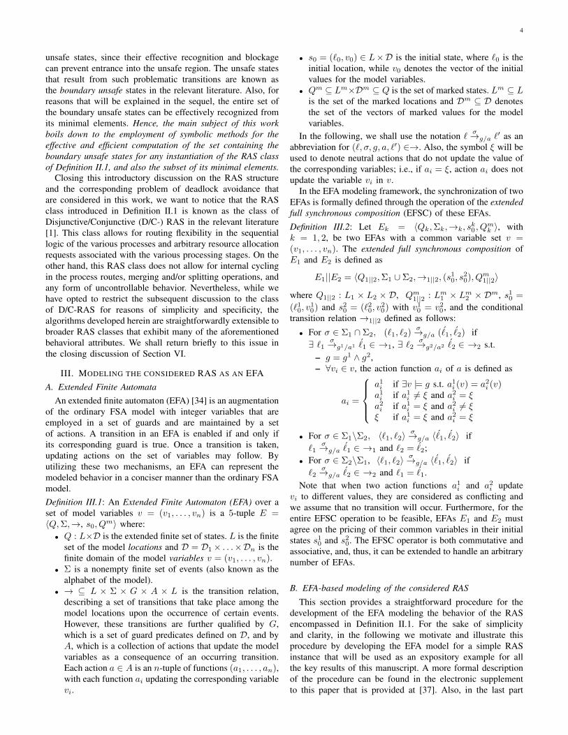
J2 : Ξ21

R1

Ξ22

R2

Ξ23

R3

Ξ24

R4

J1 : Ξ11

R4

Ξ12

R2 ∧R3

Fig. 1: The RAS configuration considered in Example III.1.

of the section, some additional remarks elaborate on theinformational content of the generated EFA, and on its (proper)interpretation in the context of the algorithmic procedures thatare the main theme of this work.

Example III.1: The RAS considered in this example isshown in Fig.1, and it comprises two process types J1 andJ2. Each process type is defined as a sequence of processingstages; the stages of process type J1 are denoted by Ξ11

and Ξ12, while the stages of process type J2 are denotedby Ξ21,Ξ22,Ξ23 and Ξ24. The set of the system resourcetypes is R = {R1, R2, R3, R4}, with capacities Ci = 1 fori = 1, 2, 3, 4. In the depicted RAS, stage Ξ12 of processtype J1 requests one unit from each of the resource typesR2 and R3 to properly support its execution. On the otherhand, stage Ξ11 of process type J1, and all stages of processtype J2, request only one unit from a single resource type;the corresponding resource types are depicted in Fig.1 next toeach of these stages.

Next, we focus on the development of an EFA modelingthe behavior of process type J1. An EFA model for processtype J2 can be developed and interpreted similarly.

Declaration of the resource variables. For each resourcetype Ri ∈ R, i = 1, 2, 3, 4, of the considered RAS, we intro-duce a resource variable vRi to trace the number of available(or free) units of Ri. The domain of vRi is {0, . . . , Ci}, whereCi is the capacity of Ri and, for this example, it is equalto one. Furthermore, since, under proper RAS operation, theinitial and the target states correspond to the RAS empty state,we set the initial and the marked value of each variable vRiequal to Ci.

Representation of the process sequential logic by asingle-location EFA. Next, we proceed to build an EFA thatcaptures the evolution of any process instance from processtype J1 through its various processing stages. The EFA modelconstructed at this phase concerns only the representationof the routing possibilities of these process instances, and itdoes not address the relevant resource allocation function; thisfunction will be modeled in a subsequent phase.

As indicated in Fig. 2, the constructed EFA has only onelocation, and its two transitions correspond to the process-initiation (or loading – 〈load, Ξ11〉) and the process-advancing(〈Ξ11, Ξ12〉) events that appear in the sequential logic of processtype J1. On the other hand, since a process instance that hasreached its final stage can always leave the system withoutposing any further resource requests, the process-termination(or unloading) event is modeled only implicitly through theevent 〈Ξ11, Ξ12〉 that models the process access to its terminalstage. Furthermore, we define a set of instance variables,

J1

〈Load, Ξ11〉g : vR4 ≥ 1;

a : v11 := v11 + 1;

vR4 := vR4 − 1

〈Ξ11, Ξ12〉g : v11 ≥ 1 ∧

vR2 ≥ 1 ∧ vR3 ≥ 1

a : v11 := v11 − 1;

vR4 := vR4 + 1

Fig. 2: The EFA modeling process type J1.

vij , that count the number of process instances executing atthe corresponding processing stages Ξij that are explicitlyrecognized by the model; hence, for this example, only oneinstance variable, v11, is defined. By making use of thisinstance variable, we can construct the necessary guards andactions for the EFA transitions. As depicted in Fig. 2, theguards determine whether a process-advancing event can takeplace, on the basis of the process availability at the originatingstage. Upon the occurrence of such an event, the correspondingactions update accordingly the number of the process instancesat the involved stages.4

Representation of the resource allocation function andits induced dynamics. Fig. 2 also shows the role of theresource allocation variables in the EFA that models thecomplete behavior of process type J1. More specifically, theresource allocation requests that are posed by the variousprocessing stages, are modeled by additional guards andactions associated with the corresponding EFA transitions;these guards and actions are highlighted by a boxing frame inFig. 2. As a more concrete example, consider the transitionlabeled by 〈Ξ11, Ξ12〉 in the EFA depicted in Fig. 2. Toexecute this transition, the associated guard requires not onlythe presence of an available process instance at stage Ξ11,but also the availability of a free unit from each of theresource types R2 and R3. Similarly, upon the execution ofthis transition, besides the updating of the number of processinstances at stage Ξ11, the augmented version of the relevantaction function updates also the resource variables to reflectproperly the new resource allocation state. For this example,since stage Ξ12 is the terminal stage of process type J1,and the unloading event is only implicitly modeled throughevent 〈Ξ11, Ξ12〉, the relevant action function simply releasesthe previously allocated unit of resource R1.

The general modeling procedure. Generalizing from theprevious example, the basic procedure that converts a given

4 As already discussed, the considered EFA model for process type J1does not avail of a variable v12 since it is assumed that a process instancereaching stage Ξ12 is (eventually) unloaded from the system, without the needfor any further resource allocation action. However, we should further clarifythat the omission of the terminal stage Ξ12 from the developed EFA model isjustified on the assumption that these EFA models of the RAS process types,and the corresponding analysis that is pursued in this paper, focus only on theissue of deadlock avoidance. Terminal processing stages cannot be involved inthe formation of deadlock, and therefore, they do not necessitate an explicitconsideration. It is implicitly assumed, though, that the system (controller)keeps track of the physical presence of any active process instances in theseterminal stages and of any temporary blocking effects that are incurred bythis presence. From a more methodological standpoint, the omission of theterminal processing stages from the developed EFA models is in line withthe “projection” operation that eliminates a subset of processing stages in theDAP synthesis methods that are presented in [23], [41].

6

RAS instance Φ = 〈R, C,P,A〉 to the corresponding EFAE(Φ) modeling the dynamics of Φ, can be summarizedby the following three stages: (i) The procedure starts bydefining the set of resource variables {vR1, . . . , vRm} thatmonitor the numbers of available units of the resource typesR = {R1, . . . , Rm} during the evolution of the resourceallocation state of Φ. (ii) Subsequently, the sequential logicof each process type Jj in P is modeled by a single-locationEFA Ej . To capture the execution of a single process instanceof Jj , a set of variables, vjk, is defined and utilized to constructthe necessary guards and actions. These variables are in one-to-one correspondence with the non-terminal stages Ξjk in thecorresponding set Sj , and each of them traces the number ofprocess instances that are executing the corresponding pro-cessing stage. The domain of integer values for each instancevariable vjk is defined as {0, . . . , θjk}, and the minimum valueof 0 is, both, the initial and the marked value for each vjk. Onthe other hand, the maximum value θjk that is associated withinstance variable vjk can be set to any upper bound for thenumber of process instances that can simultaneously executeprocessing stage Ξjk. Such a bound, that is implied by thecapacities of the resource types utilized by processing stageΞjk, can be easily computed as follows:

θjk = mini{⌊ CiAjk[i]

⌋: Ajk[i] > 0}. (1)

(iii) In order to represent the dynamics of the resource allo-cation that takes place at the different processing stages ofJj , the EFA Ej are augmented with the resource variables{vR1, . . . , vRm}, and the guards and actions of the transitionsof Ej are extended to consider and maintain the informa-tion that is contained in these new variables. Regarding themaintenance of the resource variables, the augmented EFAimplement the following logic: If the executed transition in Ejcorresponds to the process-initiating event 〈Jj loading, Ξjk〉,then it is adequate to merely allocate the resources that arenecessary for the execution of the initial processing stageΞjk. On the other hand, if the transition-labeling event isan event 〈Ξjk, Ξjk′〉 advancing an already initiated processinstance from its current stage Ξjk to a subsequent stage Ξjk′ ,the detailed updating of the resource variables depends onwhether stage Ξjk′ is a terminal stage for process type Jj . Ifit is, there is no need for (explicitly) allocating the resourcesrequested by the executing instances at stage Ξjk′ , and thecorresponding updating of the resource variables only releasesthe resources allocated to the advancing process instance whileat stage Ξjk. On the other hand, if stage Ξjk′ is non-terminal,we also need to explicitly allocate the necessary resourceunits for the execution of this stage, updating accordingly thecorresponding resource variables. (iv) Finally, the resource al-location dynamics generated by RAS Φ are formally expressedby the extended full synchronous composition (EFSC) thatcomposes the aforementioned EFA Ej to the “plant” EFAE(Φ); i.e., E(Φ) = E1|| . . . ||En. The reader is referred to[37] for a more formal description of this entire procedure.

Some further remarks. Closing this section on the rep-resentation of the considered RAS dynamics in the EFAmodeling framework, we need to elaborate further on the

way that these dynamics are captured by the generated EFAE(Φ), since these elaborations provide necessary context forthe algorithms that are developed in the following section.

We begin this discussion by noticing that every legitimateresource allocation state of the considered RAS must adhereto the restrictions that are imposed by the limited capacities ofthe system resources. In the representation of the EFA E(Φ),these restrictions are expressed by the following constraintson the pricing of the model variables vjk, j = 1, . . . , n, k =1, . . . , l(j), and vRi, i = 1, . . . ,m:

∀i ∈ {1, . . . ,m}, vRi+n∑j=1

∑k∈{1,...,l(j)}\T (j)

Ajk[i]∗vjk = Ci.

(2)In (2), we have taken into consideration the fact that

terminal processing stages are not explicitly accounted for inthe considered EFA model (for the reasons explained earlier).From a more technical standpoint, the constraints of (2) canbe perceived as a set of (resource-induced) invariants thatmust be observed by the dynamics of the EFA E(Φ) inorder to provide a faithful representation of the actual RASdynamics. Hence, in the following, we shall characterize astate s of the EFA E(Φ) with a variable vector v satisfyingthe constraints of (2), as a feasible state. Furthermore, thereader can easily verify that any execution of the EFA E(Φ)that starts from some feasible state s and evolves the stateaccording to the transition-firing logic that is encoded in thisautomaton, maintains the state feasibility.5 In particular, sincethe initial state s0 of the considered EFA has vjk = 0, ∀j, k,and vRi = Ci, ∀i, s0 is a feasible state, and all the statesthat are reachable from it (known as the reachable state spaceof E(Φ)) are also feasible. This last remark implies that theEFA E(Φ) provides, indeed, a faithful representation of thedynamics of the underlying RAS Φ.

On the other hand, the specification of the state set Q asQ = L ×

∏iD(vRi) ×

∏j,k D(vjk), where the domain sets

D(v) of the various variables v are determined as described inthe previous paragraphs, implies that Q may contain infeasiblestates, as well. Since these states remain unreachable in anyproper execution of E(Φ), they do not compromise the analyt-ical power of this model regarding the traced RAS dynamics.Yet, these states might still be a nuisance in the computationsthat are effected by the presented algorithms, since they mightencumber these computations with excursions to state regionsthat are irrelevant to the actual system dynamics. Wheneverthis problem arises, it can be addressed by “filtering” therelevant state subsets for state feasibility. In Section IV weshall provide a more specific implementation of such a filteringmechanism that is appropriate for the symbolic computationthat is pursued in that section.

Example III.2: Fig. 3 depicts the dynamic behavior encodedby the EFA E(Φ) that was developed for the RAS instancein Example III.1. The depicted state transition diagram (STD)includes only the RAS feasible states that are reachable fromthe initial state of E(Φ), and furthermore, it considers onlythose states that are modeled explicitly in this EFA through

5A formal proof of this fact can be easily constructed as an inductiveargument that is based on the length of the executed trace.

7

0000 1111

s0

1000 1110

s1

0100 0111

s2

1100 0110

s3

0001 1101

s4

1010 1010

s5

1001 1100

s6

1110 0010

s7

1101 0100

s8

1011 1000

s9

1111 0000

s10

0101 0101

s11

0110 0011

s12

0011 1001

s13

0010 1011

s14

0111 0001

s15〈load, Ξ11〉 〈Ξ11, Ξ12〉

〈load, Ξ21〉

〈load, Ξ11〉 〈Ξ11, Ξ12〉

〈load, Ξ21〉

〈Ξ21, Ξ22〉

〈Ξ23, Ξ24〉

〈load, Ξ11〉 〈Ξ22, Ξ23〉〈load, Ξ21〉

〈load, Ξ21〉

〈Ξ22, Ξ23〉 〈Ξ21, Ξ22〉〈load, Ξ21〉

〈Ξ23, Ξ24〉

〈load, Ξ11〉

〈load, Ξ21〉

〈Ξ21, Ξ22〉

〈Ξ22, Ξ23〉

〈Ξ23, Ξ24〉

〈load, Ξ21〉

〈load, Ξ11〉

〈Ξ23, Ξ24〉

〈load, Ξ11〉

〈load, Ξ21〉

〈Ξ22, Ξ23〉

〈load, Ξ11〉

〈load, Ξ11〉

〈Ξ21, Ξ22〉

Fig. 3: The state transition diagram (STD) modeling the RAS dynamics encoded by the EFA E(Φ) that was developed forExample III.1.

the pricing of the corresponding model variables. As it can beseen in Fig. 3, the considered STD involves sixteen (16) states,denoted by si, where i = 0, . . . , 15. Each state is describedby eight components that correspond to the values of theinstances variables v11, v21, v22, v23 and the resource variablesvR1, vR2, vR3, vR4 of the EFA E(Φ). States depicted bya dashed line are unsafe. Furthermore, for reasons that willbecome clear in the following, the transitions in the depictedSTD are partitioned into two subsets that collect respectivelythe transitions corresponding to “process initiation” (or “load-ing”) and “process advancement” events. These two subsetsof transitions are depicted respectively as dashed and solidtransitions in the STD of Fig. 3.

IV. COMPUTING THE MINIMAL BOUNDARY UNSAFESTATES

A. Binary Decision Diagrams and Symbolic Computation

Binary decision diagrams (BDDs) [27] are a memory-efficient data structure used to represent Boolean functionsas well as to perform set-based operations. The field incomputer science that studies the employment of BDDs in thesupport of the aforementioned tasks has come to be known as“symbolic computation”, and a systematic exposition of therelevant theory can be found, for instance, in [42], [43]. Inthe next paragraphs we introduce some theoretical conceptsand elements pertaining to BDDs and symbolic computationthat provide necessary background and context for the maindevelopments of this section.

To present the basic BDD theory employed in this work, inthe following, we set B ≡ {0, 1}. Also, for any Boolean func-tion f : Bn → B, in n Boolean variables X = (x1, . . . , xn),we denote by f |xi=0(resp. 1) the Boolean function that isinduced from function f by fixing the value of variable xito 0 (resp. 1). Then, a BDD-based representation of f is agraphical representation of this function that is based on thefollowing identity:

∀xi ∈ X, f = (¬xi ∧ f |xi=0) ∨ (xi ∧ f |xi=1) (3)

More specifically, (3) enables the representation of theBoolean function f as a single-rooted acyclic digraph withtwo types of nodes: decision nodes and terminal nodes. Aterminal node can be labeled either 0 or 1. Each decisionnode is labelled by a Boolean variable and it has two outgoingedges, with each edge corresponding to assigning the value ofthe labeling variable to 0 or to 1. The value of function f forany given pricing of the variable set X is evaluated by startingfrom the root of the BDD and at each visited node followingthe edge that corresponds to the selected value for the node-labeling variable; the value of f is the value of the terminalnode that is reached through the aforementioned path.

The size of a BDD refers to the number of its deci-sion nodes. A carefully structured BDD can provide a morecompact representation for a Boolean function f than thecorresponding truth table and the decision tree; frequently, theattained compression is by orders of magnitude.

From a computational standpoint, the power of BDDs liesin the efficiency that they provide in the execution of binary

8

operations. Let f and f ′ be two Boolean functions of X . Then,it should be evident from (3) that a binary operator ⊗ between(the BDDs representing) f and f ′ can be recursively computedas

f⊗f ′ = [¬x∧(f |x=0⊗f ′|x=0)]∨ [x∧(f |x=1⊗f ′|x=1)] (4)

where x ∈ X . If dynamic programming is used, the compu-tation implied by (4) can have a complexity of O(|f | · |f ′|)where |f | and |f ′| are the sizes of (the BDDs representing) fand f ′.

A particular operator that is used extensively in the fol-lowing is the existential quantification of a function f overits Boolean variables. For a variable x ∈ X , the existentialquantification of f is defined by ∃x.f = f |x=0∨f |x=1. Also,if X = (x1, . . . , xk) ⊆ X , then ∃X.f is a shorthand notationfor ∃x1.∃x2. . . .∃xk.f . In plain terms, ∃X.f denotes all thosetruth assignments of the variable set X\X that can be extendedover the set X in a way that function f is eventually satisfied.

B. EFA encoding through BDDs.

To represent an EFA E by a Boolean function, different setsof Boolean variables are employed to encode the locations,events and integer variables. For the encoding of the state setQ : L × D, we employ two Boolean variable sets, denotedby XL and XD = XD1 ∪ . . . ∪XDn , to respectively encodethe two sets L and D. Then, each state q = (`, v) ∈ Q isassociated with a unique satisfying assignment of the variablesin XL ∪ XD. Given a subset Q of Q, its characteristicfunction χQ : Q → {0, 1} assigns the value of 1 to allstates q ∈ Q and the value of 0 to all states q /∈ Q.6 Thesymbolic representation of the transition relation → relies onthe same idea. A transition is essentially a tuple 〈`, v, σ, `′, v′〉specifying a source state q = (`, v), an event σ, and a targetstate q′ = (`′, v′). Formally, we employ the variable sets XL

and XD to encode the source state q, and a copy of XL

and XD, denoted by XL and XD, to encode the target stateq′. In addition, we employ the Boolean variable set XΣ toencode the alphabet of E, and we associate the event σ with aunique satisfying assignment of the variables in XΣ. Then, weidentify the transition relation → of E with the characteristicfunction

∆(〈q, σ, q′〉) =

{1 if ` σ→g/a `

′ ∈ →, v |= g, v′ = a(v)0 otherwise

That is, ∆ assigns the value of 1 to 〈q, σ, q′〉 if there exists atransition from ` to `′ labelled by σ, the values of the variablesat ` satisfy the guard g, i.e., v |= g, and the values of thevariables v′ at `′ are the result of performing action a on v.

Given a RAS instance Φ and the distinct EFA E1, . . . , Enthat model the resource allocation dynamics of the RASprocess types J1, . . . , Jn, we shall denote by ∆1, . . . ,∆n thecorresponding symbolic representations of those EFA. Further-more, we shall denote by ∆E the symbolic representation ofE(Φ), the EFA that models the integrated dynamics of RAS Φ.We remind the reader that E(Φ) is defined as the EFSC of the

6In the rest of this document, we shall use interchangeably the originalname of a set Q and its characteristic function, χQ, in order to refer to thisset.

EFA E1, . . . , En. Hence, ∆E can be systematically obtainedfrom ∆1, . . . ,∆n through the approach for the symboliccomputation of EFSC that is presented in [33]; we refer thereader to that work for the relevant details.

We also remind the reader that, while ∆E provides asymbolic representation of the resource allocation dynamicsof RAS Φ, it also contains a subset of infeasible states thatwere described in the closing remarks of Section III. Theinfeasibility of these states can be detected by the characteristicfunction χF that expresses state feasibility in the BDD-basedrepresentational context, and it can be constructed as follows:First, the invariants of (2) are collectively expressed by thefollowing Boolean function

m∧i=1

(vRi +

n∑j=1

∑k∈{1,...,l(j)}\T (j)

Ajk[i] ∗ vjk = Ci). (5)

Then, χF is defined by the BDD that collects the binaryrepresentations of all the value sets for the variables vRi andvjk that satisfy the Boolean function of (5). As a more concreteexample, the instantiation of (5) for the example RAS of Fig. 1is as follows:

1 ∗ v11 + vR4 = 1 ∧ 1 ∗ v21 + vR1 = 1 ∧1 ∗ v22 + vR2 = 1 ∧ 1 ∗ v23 + vR3 = 1. (6)

Finally, as it will be revealed in the following, the com-putations pursued in this work do not require the explicitrepresentation of the event set Σ = Σ1 ∪ . . . ∪ Σn. Hence, toreduce the number of Boolean variables employed by ∆E, inthe following we will suppress from ∆E the Boolean variableset XΣ

E , that represents Σ. In addition, since the locations ofthe considered EFA do not convey any substantial informationother than characterizing the various process types as modelentities with a distinct behavior modeled by the correspondingEFA, ∆E can be further compressed by suppressing theBoolean variable set XL

E = XL1 ∪ . . . ∪ XL

n , as well. Theelimination of the aforementioned sets of variables from∆E is technically effected through the following existentialquantification:

∆E := ∃(XΣE ∪XL

E).∆E (7)

In the rest of this work, when we refer to the plant model ∆E

we shall imply the output of the operation performed in (7).The following three subsections assume the availability

of an appropriately constructed BDD ∆E that is a validrepresentation of the composed EFA E(Φ) = E1|| . . . ||Enand has been compressed through the existential quantificationexpressed in (7), and proceed to present a series of sym-bolic algorithms for the computation of the set of (minimal)boundary unsafe states in the considered RAS. As remarkedin Section I, the presented developments provide two differentalgorithms for retrieving all the boundary unsafe states withinthe underlying RAS state-space, and an additional algorithmfor identifying and removing non-minimal elements from thisset.

9

Algorithm 1: Symbolic computation of the reachableboundary unsafe statesInput: ∆E and χ{s0}Output: χRB

1 χR := χ{s0}2 repeat // compute the set of reachable states, χR3 χRpre := χR4 χRcur := ∃XD.(χR ∧∆E)

5 χR := χRpre ∨ (χRcur [XD → XD])

6 until χR = χRpre

7 χC := χ{s0}8 repeat // compute the set of safe states, χC9 χCpre

:= χC

10 χCcur := ∃XD.(χC [XD → XD] ∧∆E)

11 χC := χCpre ∨ χCcur

12 until χC = χCpre

13 χRC := χR ∧χC // compute the reachable ∧ safe state set// finally, compute the set of boundary unsafe states, χRB

14 ∆B := χRC ∧∆E

15 χB := (∃XD.∆B)[XD → XD]

16 χRB := χB ∧ ¬χC

C. An extension of the standard SCT synthesis algorithm forthe computation of reachable boundary unsafe states

The first algorithm for the computation of the RAS bound-ary unsafe states that is developed in this work is depicted inAlgorithm 1, and it constitutes an adaptation of the generalalgorithm that has been developed by the SCT for supportingmaximally permissive non-blocking supervision. More specif-ically, given the symbolic representation of the composedtransition relation ∆E that is defined by (7), and the corre-sponding characteristic function χ{s0} representing the initialand marked state of the EFA E(Φ),7 Algorithm 1 computesthe characteristic function of the reachable boundary unsafestate set, χRB , through the following symbolic operations.

The algorithm starts with the computation of a symbolic rep-resentation of the reachable state set χR, through the forwardsearch depicted in Lines 1-6. For that, the algorithm employstwo characteristic functions χRpre

and χRcurto respectively

represent (i) the state set χR already reached at the beginningof each iteration of the forward-search process, and (ii) the setof states that can be reached from the current elements of χRthrough a single transition of ∆E. The reachable state set χRkeeps expanding with the new states entering χRcur at eachiteration, until no new reachable state can be computed. AtLine 5, the operation [XD → XD] denotes the replacementof all variables of XD by those of XD, so that the reachablestates identified at each iteration are eventually represented byXD and the forward search can continue. The characteristicfunction of the co-reachable state set, denoted by χC , can be

7Since the Boolean variable set representing the locations of the originalEFA ∆E has been existentially quantified, s0 is just equal to the vector ofthe initial (and also the marked) values for the variables.

computed in a similar manner. The corresponding backwardsearch is depicted in Lines 7-12 of Algorithm 1.

As remarked in Section II, in the RAS literature, co-reachable states are also referred to as safe states, and statesthat are not co-reachable are characterized accordingly asunsafe. The set B of boundary unsafe states can be formallyexpressed as B ≡ {u | ∃ s → u in ∆E s.t. s ∈ χC and u /∈χC}. Having obtained the characteristic functions χR and χC ,the characteristic function of the reachable safe state set, χRC ,can be obtained through the conjunction depicted at Line 13.On the other hand, to compute the characteristic function ofthe reachable boundary unsafe state set χRB , Algorithm 1 firstretrieves from ∆E all the transitions with their source statebelonging to χRC . The set of these retrieved transitions isdenoted by ∆B , and its computation is carried out in Line 14of the algorithm. Subsequently, Line 15 collects in χB the setof the target states of the transitions extracted in ∆B . Finally,in Line 16, the characteristic function χRB is computed byremoving from set χB all the safe states, i.e., all those statesthat also belong in χC .

It is clear from the above discussion that Algorithm 1terminates in finite time. Also, since this algorithm reliesextensively on standard procedures developed by SCT forestablishing maximally permissive non-blocking supervision,a formal proof for its correctness can be based on argumentsprovided in the corresponding SCT literature, and we refer tothat literature for the relevant details (c.f., for instance, [12],[13], [33]).

Example IV.1: As a concrete example, we apply Algorithm 1to the STD depicted in Fig. 3. The transitions of the STD aresymbolically represented in the BDD ∆E(J1)||E(J2), whereE(J1) and E(J2) are the EFA modeling the process typesJ1 and J2 of the RAS instance depicted in Fig. 1. Startingwith χR := {s0}, the computation of Lines 2-6 will returnthe set χR containing all of the sixteen reachable states s0

– s15. On the other hand, the set χC obtained from thecomputation in Lines 7-12 will contain all the safe statess0 – s4, s11 – s15 depicted in Fig. 3, and possibly someadditional safe but unreachable states (not depicted in Fig. 3).The subsequent conjunction of χC with χR in Line 13 filtersout the unreachable safe states from χC ; i.e., the returned setχRC contains only the reachable and safe states s0 – s4, s11

– s15 depicted in Fig. 3.8 Finally, the algorithm operations inLines 14-16 will return the set χRB containing the states s5 –s10, i.e., all the reachable and unsafe states depicted in Fig. 3,since all these states can be reached from some reachable safestate in χRC in one transition.

8In fact, the EFA E(Φ) corresponding to the RAS considered in thisexample does not contain any feasible unreachable states. This can be estab-lished by noticing that in the considered RAS class, any feasible unreachablestates essentially result by “swapping” (i.e., simultaneously advancing) processinstances that are in deadlock. But in the semantics of the EFA E(Φ) ofSection III, any deadlock must involve some process instance of type J1,and the aforementioned swapping of these process instances implies theirimmediate unloading from the system.

10

D. An alternative algorithm for the computation of feasibleboundary unsafe states

In this subsection, we present an alternative symbolic al-gorithm that decomposes the computation of the boundaryunsafe states into two stages. In the first stage, all the deadlockstates w.r.t. the advancement events in the considered RASare identified and computed from the symbolic representationof the state space, ∆E. In the second stage, the deadlockstates are used as starting points for a search procedure over∆E that identifies all the boundary unsafe states. The entirecomputation is formally expressed by Algorithm 2, that workswith the BDDs of ∆E and the characteristic function χF ,9

and returns the characteristic functions χFD and χFB thatconstitute respective symbolic representations of the sets ofthe feasible deadlock states and the feasible boundary unsafestates. In general, the set χFB obtained from the presentedalgorithm may include some states that are not reachablefrom the initial state s0; i.e., in general, χRB 6= χFB butχRB ∧ χFB = χRB . Hence, the presence of any additionalstates in the set χFB does not impede the implementationof the maximally permissive DAP by means of this set andthe one-step-lookahead logic that was outlined in the earlierparts of this manuscript. Furthermore, for reasons that willbecome clear in the following, it is pertinent to assume that thecharacteristic function ∆E is partitioned in the characteristicfunctions ∆A and ∆L that collect respectively the transitionsin ∆E corresponding to process advancement and processloading events; obviously, ∆E = ∆A ∨ ∆L. The rest of thissection elaborates on the various phases of the computationthat is depicted in Algorithm 2, and establishes formally itscorrectness.

Identification of the feasible deadlock states. The sym-bolic operations for the computation of the characteristicfunction χFD are depicted in Lines 1-4 of Algorithm 2, andthey can be described by the following two steps:1) The first step consists of Lines 1-3 in Algorithm 2 and itcomputes the characteristic function χD of all the (partial)deadlock states in ∆E, i.e., those states that are differentfrom the initial state s0 and they do not enable any process-advancing events. This function is computed by first extractinginto the characteristic function χT all the target states from∆A ∨ ∆L (i.e. from ∆E) and in the characteristic functionχE all the states that enable process-advancing events. Sub-sequently, χD is computed as the elements of χT that are notin χE (i.e., they do not enable any process-advancing events)or the initial state s0.2) Since χD is computed from the entire set of transitionsthat is contained in ∆E, it might contain deadlock states thatare infeasible (i.e., they violate the resource-induced invariantsof (2)). The presence of these infeasible states in χD wouldincrease unnecessarily the computational cost of the secondstage of the considered algorithm, that utilizes the identifieddeadlock states as starting points for the identification of theadditional set of deadlock-free unsafe states. Hence, in the laststep of the first stage of Algorithm 2, the obtained state setχD is filtered through its conjunction with the characteristic

9We remind the reader that χF characterizes the feasibility of the variousstates encountered in ∆E w.r.t. the resource-induced invariants of (2).

function χF in order to obtain the set of feasible deadlockstates; this set is represented by the characteristic functionχFD.

Example IV.2: The application of Lines 1-4 of Algorithm 2to the BDDs ∆A and ∆L corresponding to the STD depictedin Fig. 3, will return the BDD of feasible deadlock states,χFD, that includes the states s6, s9 and s10. Indeed, it can beclearly seen in the depicted STD that no solid edges emanatefrom these three states; i.e., these states enable no process-advancing events. The reader should also notice that states s6and s9 do enable process-loading events; but these events donot contribute to the progress of the already initiated processinstances, and they only aggravate an already problematicsituation. Finally, we also remind the reader that, according toFootnote 8, the EFA E(Φ) corresponding to this example doesnot contain any feasible unreachable states, and therefore, theaforementioned three states is the entire content of the state-setencoded by the BDD χFD that is returned at Line 4.

Computation of the feasible boundary unsafe states.Having obtained the set χFD of the feasible deadlock states,the algorithm proceeds with the symbolic computation of thefeasible boundary unsafe states in the RAS state-space ∆E.These states are collected in the characteristic function χFB ,which is computed in Lines 5-18 of Algorithm 2. A detaileddescription of this computation is as follows:1) At this phase of the computation, Algorithm 2 employsthe set U in order to collect all the identified unsafe states.Furthermore, at each iteration, the set Unew defines the setof the unsafe states that are to be processed at that iteration,through one-step-backtracking in ∆A, in an effort to reachand explore new states. The corresponding symbolic repre-sentations for these two sets, denoted by χU and χUnew , areinitialized to χFD. Finally, we also define the transition setUpre ≡ {(s, u) ∈ ∆A | u ∈ U ∧ s /∈ U}; i.e., during theentire search process, Upre contains the transitions of ∆A

where the target states belong to U while the source stateshave also transitions to states that currently are not in U . Thecharacteristic function of Upre is initialized to zero.2) During the main iteration of the executed search process, thealgorithm first extracts all the states that can be reached fromthe unsafe state set Unew by tracing backwards some process-advancing transition in ∆A. This computation is performedin Lines 7-8 of the algorithm, with the extracted states repre-sented by the characteristic function χSU . Also, the backtracedtransitions of ∆A are represented by the characteristic function∆U .3) Subsequently, Algorithm 2 tries to resolve which of thestates collected in χSU can be classified as unsafe. Thisresolution is performed in Lines 9-11 of the algorithm. Morespecifically, the algorithm first collects in the transition set∆SA all those process-advancing transitions of ∆A that em-anate from states in χSU . Subsequently, it removes from ∆SA

those transitions that are known to lead to unsafe states,namely the transitions that are also in ∆U and in Upre. Thesource states for any transitions remaining in ∆SA after thislast operation are collected in χNU ; these are states that havetransitions leading to states currently not in U , and therefore,they cannot be classified as unsafe (at least in this iteration).

11

Algorithm 2: Symbolic computation of the boundary unsafe statesInput: ∆E (as ∆A ∨∆L) and χFOutput: χFB/* Compute the feasible deadlock states χFD */

1 χT :=(∃XD. (∆A ∨∆L)

)[XD → XD] // χT collects the target states in the transitions of ∆E;

2 χE := ∃XD. ∆A // χE contains the states of ∆A that enable advancement events;3 χD := χT ∧ ¬χE ∧ ¬χ{s0} // χD is the set of deadlock states w.r.t. advancement events, including infeasible states;4 χFD := χD ∧ χF // χFD is the set of feasible deadlock states w.r.t. advancement events;

/* Compute the feasible boundary unsafe states χFB from χFD */5 χUnew

:= χFD, χU := χFD,∆Upre:= 0 // initialization;

6 repeat7 ∆U := χUnew

[XD → XD] ∧∆A // ∆U contains the transitions in ∆A where the target states belong to χUnew;

8 χSU := ∃XD. ∆U // χSU contains the source states of ∆U ;9 ∆SA := χSU ∧∆A // ∆SA contains the transitions in ∆A where the source states belong to χSU ;

10 χNU := ∃XD. (∆SA ∧ ¬∆U ∧ ¬∆Upre) // χNU contains the states in χSU that are not qualified as

// unsafe states at the current iteration;11 χUcur

:= χSU ∧ ¬χNU // χUcurcontains the unsafe states at the current iteration;

12 χUnew := χUcur ∧ ¬χU // χUnew contains the newly computed unsafe states, which are used for the next iteration;13 χU := χU ∨ χUcur

// χU accumulates the unsafe states in χUcur;

14 ∆Upre:= (∆Upre

∨∆U ) ∧ ¬χUcur// ∆Upre

is updated by first adding the transitions in ∆U and then// removing the transition with the source states in χUcur

;15 until χUnew = 0

16 ∆B := χU [XD → XD] ∧∆E // ∆B contains the transitions with the target states belonging to χU ;17 ∆SB := ∆B ∧ (¬χU ) // ∆SB contains the transitions in ∆B where the source states are safe states;

18 χFB := (∃XD. ∆SB)[XD → XD] // χFB is obtained by extracting the set of target states of ∆SB;

On the other hand, the complement of χNU w.r.t. the overallset of extracted states χSU must contain states with all theiremanating transitions leading to unsafe states, and therefore,they are themselves unsafe; these states are identified andcollected in set χUcur in Line 11.

4) Lines 12-14 perform the necessary updates so that all thecritical data structures represent correctly the current outcomeof the ongoing search process. Hence, Line 12 removes fromχUcur any states that have already been classified as unsafe inthe previous iterations; the remaining states are the elementsof Unew for the next iteration. Line 13 adds to the setU the newly identified unsafe states, and finally, Line 14updates the transition set Upre; this last update is performedby initially adding to Upre all the transitions in ∆U (i.e., thetransitions that were backtraced during the current iteration),and subsequently removing those transitions with source statesidentified as unsafe.

5) The iteration described in items (2-4) above terminateswhen no new unsafe states can be identified by the algorithm.At this point, Algorithm 2 proceeds to extract the boundaryunsafe states from set χU . For that, at Line 16, the algorithmcomputes from ∆E all the transitions with the target statesbelonging to the unsafe state set χU ; the relevant transition setis denoted by ∆B. Next, at Line 17, the algorithm retrievesfrom ∆B the transition set ∆SB, where the source states of theincluded transitions are safe states. Finally, χFB is obtained

by extracting the target states from ∆SB and performing thereplacement of XD by XD.

Example IV.3: In the context of the example STD of Fig. 3,the backward search of Algorithm 2 in order to identify all thedeadlock-free unsafe states, implemented by Lines 6-15, willstart from the identified deadlock states s6, s9 and s10, and itwill be performed on the solid transitions of this STD, i.e., ontransitions corresponding to process-advancing events. Morespecifically, at the first iteration of this search, states s5 ands8 are reached by respectively backtracing from states s6 ands9, and they are classified as unsafe since the backtraced tran-sitions leading to these states are the only process-advancingtransitions emanating from them. The second iteration setsχUnew

; = {s5, s8}, and it tries to backtrace through process-advancing transitions from these two states, in quest of newunsafe states. Indeed, this backtracing from state s8 exposesthe unsafety of state s7. On the other hand, state s3 thatis reached through the backtracing from state s5 cannot beclaimed as unsafe, since s3 also avails of transition (Ξ11,Ξ12)leading to state s2, which is not included in the current set ofunsafe states. The backward search terminates after the thirditeration since the attempt to backtrace from state s7 – i.e.,the contents of the set χUnew

in this iteration – through someprocess-advancing transitions fails to reach any states at all(and therefore, there are no newly identified states with all oftheir process-advancing transitions leading to the unsafe states

12

that were identified during the first two iterations). Finally,Algorithm 2 proceeds to extract the boundary unsafe states.Since, in this example, all unsafe states s5 – s10 can be reachedfrom the safe subspace through a single transition, the resultingstate set χFB contains all states s5 – s10. It is also importantto notice that, in the considered example, we were able toidentify correctly all the unsafe states without visiting at allthe safe states s0 – s2, s4 and s11 – s15; even for this smallexample, this unvisited area constitutes more than 50% of theentire state space.

Correctness analysis. To prove the effectiveness of Algo-rithm 2 w.r.t. the penultimate objective of the implementa-tion of the maximally permissive DAP through the one-step-lookahead scheme that was outlined in the earlier parts of thismanuscript, we need to show that (i) the algorithm terminatesin a finite number of steps, (ii) the returned set χFB containsall the feasible boundary unsafe states, and furthermore, (iii)χFB does not contain any feasible safe state.

The finiteness of Algorithm 2 depends on whether thebackward search performed in Lines 6-15 can terminate ina finite number of iterations. We notice that the terminationof this search is determined by the set of the new unsafestates, χUnew , computed at each iteration; if χUnew is empty,the backward search terminates. We also notice that the setχUnew

will finally be empty during the search, since the setof states in ∆A is finite. Hence, Algorithm 2 terminates in afinite number of steps.

The next theorem establishes the correctness of Algorithm2, by establishing items (ii) and (iii) in the above list.

Theorem IV.1. The set χFB returned by Algorithm 2 pos-sesses the following properties:

1) It contains only feasible states.2) It contains all the feasible boundary unsafe states in the

underlying RAS state-space.3) It contains no feasible non-boundary unsafe state.4) It contains no safe state.

Proof: Due to space considerations, here we provide asketch for the proof of Theorem IV.1. A complete correctnessanalysis for Algorithm 2, including a more formal proof forthe above theorem, can be found in the electronic supplementof [37].

The technical analysis of Algorithm 2 begins by establish-ing that the characteristic function χFD, obtained from thesymbolic operations performed in Lines 1-4 of Algorithm 2,identifies correctly the feasible deadlock states in the EFA thatis represented by the employed BDD ∆E.

Furthermore, since the transitions that are encoded by theEFA ∆E observe the invariants of (2), and the set χFD thatis obtained in the first computational phase of Algorithm2 contains only feasible deadlock states, it follows that allthe states that are reached by Algorithm 2 during its secondphase of backward search, are also feasible. This last remarkestablishes the first result of Theorem IV.1.

To show the validity of the remaining clauses of Theo-rem IV.1, we first establish that the set U maintained byAlgorithm 2 will contain, upon the algorithm termination, allthe feasible unsafe states and no feasible safe states of ∆E.

Hence, to show that U will contain all the feasible unsafestates of ∆E, we first notice that the finite and acyclic natureof the paths that define the execution logic of the variousprocess types in the considered RAS class, imply that thesubspace that is reached from any unsafe state u followingonly transitions in ∆A has a finite, acyclic structure. Thisremark, when combined with the presumed unsafety of state u,further implies that every path in ∆A that emanates from stateu is an acyclic path that terminates at some feasible deadlockstate. Let ζ denote the longest length of these paths, wherethe length of a path is defined by the number of the involvedtransitions. Then, the inclusion in the set U of unsafe statesu with ζ = 1 results immediately from the basic operationsin the backtracing iteration of Algorithm 2 and the alreadyestablished fact that the algorithm recognizes successfully allthe feasible deadlocks during its first phase. The inclusion inthe set U of unsafe states u with ζ > 1 can be addressed byan inductive argument on ζ.

On the other hand, the fact that the state set U does notcontain any feasible safe states of ∆E can be establishedby a simple induction on the number of iterations that areperformed by the algorithm, while considering the role that isplayed by the set Upre in the algorithm computations.

In view of the above results, to obtain result #2 of Theo-rem IV.1 it suffices to show that the construction of the setFB in Lines 16-18 of Algorithm 2 retains all the boundaryfeasible unsafe states in U . But this can be easily checkedfrom the facts that (a) the transition set ∆B contains all thetransitions with target states in set U , while (b) the transitionset ∆SB is obtained from ∆B by removing only transitionswith source states in U (and therefore, unsafe, according tothe previous discussion).

Result #3 of Theorem IV.1 is also inferred from the con-struction of the set ∆SB from the set ∆B through the removalof all those transitions with source states in U , upon noticingthat U contains all the feasible unsafe states of ∆E.

Finally, Result #4 of Theorem IV.1 is obtained from thefacts that the state set U does not contain any feasible safestates and all the transitions in the set ∆B have target statesin U .

E. Computing the minimal boundary unsafe states

An important implication of the invariants of (2) is that,at any feasible state of the RAS state-space, the values ofthe resource variables vRi can be induced from the values ofthe instance variables vjk. In other words, any feasible states of the considered RAS can be uniquely determined onlyby the specification of its instance variables vjk. Hence, onecan obtain a more compact symbolic representation of the setof feasible boundary unsafe states, χFB , that is computed byAlgorithm 2, by eliminating from the elements of χFB thevalues that correspond to the variables vRi.10 Letting XR

10We notice, however, that the presence of the variables vRi during theexecution of Algorithm 2 is instrumental for ensuring some of the propertiesthat were established in Theorem IV.1, especially Property 1. Also, whilewe carry out the subsequent discussion in the context of the set FB that isreturned by Algorithm 2, similar remarks and techniques apply to the set RBthat is returned by Algorithm 1.

13

denote the Boolean variables representing the values of theresource variables vRi, i = 1, . . . ,m, this elimination can beperformed through the following existential quantification:

χFB := ∃XR. χFB . (8)

The compressed representation of the set χFB that isobtained through (8) becomes even more important whennoticing that, according to [41], state unsafety is a monotoneproperty in this representation. More specifically, given anytwo feasible boundary unsafe states u1, u2 represented ac-cording to the logic of (8), we consider the ordering relation“≤” on them that is defined by the application of this relationcomponentwise; i.e.,

u1 ≤ u2 ⇐⇒ (∀k = 1, . . . ,K, u1[k] ≤ u2[k]), (9)

where u1[k] and u2[k] are the values of the k-th instancevariable for u1 and u2. Furthermore, we use the notation ‘<’to denote that condition (9) holds as strict inequality for atleast one component vk ∈ {v1, . . . , vK}. It is shown in [41]that if state u1 is unsafe and state u2 satisfies u1 ≤ u2, thenstate u2 is also unsafe. Hence, under the state representationof (8), the set FB can be effectively defined by the subset ofits minimal elements; we shall denote this subset by FB, i.e.,FB ≡ {u ∈ FB | @u′ ∈ FB s.t. u′ < u}.

The results of our computational experiments that arereported in Section V reveal that the TRIE data structuresthat provide effective representation of the sets FB, areconsiderably more compact, in terms of the employed numberof nodes, than the TRIE data structures that encode the originalsets FB. Hence, there seems to be substantial advantage inthe representation of the forbidden RAS states, during thedeployment of the one-step-lookahead scheme of [24], bymeans of the sets FB. In the context of this work, we havealso developed a symbolic algorithm for the extraction ofthe set FB from its parent set FB; we shall refer to thisalgorithm as “Algorithm 3” in the sequel. Since, however,the symbolic computation of the minimal elements of a givenset of vectors, like that of FB, is a more generic task thanthe RAS-related concepts and computation that are pursuedin this work, we have opted to include this material in theelectronic supplement of this paper [37], and we refer theinterested reader to that resource for a complete and systematicexposition of the corresponding results.

V. COMPUTATIONAL RESULTS AND EVALUATION

The EFA-based modeling procedure for the consideredRAS and the collection of the symbolic algorithms for thecomputation of their minimal boundary unsafe states thatwere developed in this work, have been implemented in theDES software tool Supremica [36]. The program is writtenin Java and it uses JavaBDD [44] with BuDDy as the BDDlibrary. In this section, we report the results from a series ofcomputational experiments11 in which we applied the symbolicalgorithms of Section IV on a number of randomly generatedinstantiations of the RAS class that was defined in Section II.Each of the generated instances is further specified by:

11The experiments were carried out on a standard desktop, (2.66 GHz IntelCore Quad CPU, 10GB RAM) running Windows 7

• The number of resource types in the system; the rangeof this parameter is between 3 and 16.

• The capacities of the resource types in the system; therange of this parameter is between 1 and 4.

• The number of process types in the system; the range ofthis parameter is between 3 and 5.

• The number of processing stages in each process; therange of this parameter was between 3 and 16. Fur-thermore, in order to remain consistent with the RASstructure defined in Section II, no processing stage has azero resource-allocation vector.

• The structure of the process graphs Gi and the resourcerequest vectors supported by the resource allocation func-tion A. In terms of the structure of Gi, the generated ex-amples contain RAS instances where all processes followsimple linear flows, as well as RAS instances where someprocesses possess routing flexibility (Disjunctive RAS).In terms of the resource request vectors, our examplescontain RAS instances with either single-type resourceallocation or conjunctive resource allocation (ConjunctiveRAS).

Table I reports a representative sample of the results ob-tained in our experiments. The first section in the table is forRAS instances with simple linear process flows and single-unit resource allocation (from a single resource type) for eachprocessing stage. The second section is for RAS instanceswith simple linear process flows and conjunctive resourceallocation for each processing stage. Finally, the last sectionof the table is for RAS instances with conjunctive resourceallocation for each processing stage, but also routing flexibility.In the experiments, first we constructed the necessary BDDsmodeling the underlying EFA for the aforementioned RASinstances, then we applied Algorithms 1 and 2 to these BDDsto obtain all the boundary unsafe states, and subsequently weapplied Algorithm 3 to remove the non-minimal unsafe statesfrom the set of boundary unsafe states. Finally, we also appliedthe algorithm of [35] to the BDDs returned by Algorithms 2and 3 in order to convert these BDDs into the TRIEs that willsupport the final implementation of the maximally permissiveDAP (c.f. the relevant discussion in the previous sections).

Columns 1-2 in Table I report respectively the cardinalitiesof the set of reachable states, R, and the set of the Booleanvariables, XD, that are employed by the BDD ∆E which is theprimary input to Algorithms 1 and 2. Since, in classical SCT,the maximally permissive DAP is characterized by the trimof the corresponding RAS-modeling FSA, |R| can functionas a pertinent surrogate measure of the problem complexity,when it is solved through a conventional representation of thisFSA. On the other hand, (7) implies that |XD| is equal tothe number of binary variables that are necessary to encodethe resource capacities and (an upper bound to) the maximalnumber of process instances that can occupy each of the non-terminal processing stages of the considered RAS instanceΦ, and therefore, it can be perceived as a surrogate measureof the “size” of Φ in terms of its structural elements (c.f.Definition II.1). Also, in the world of symbolic computation,the number of the Boolean variables that is communicated by|XD|, is frequently used as a practical surrogate measure of

14

TABLE I: A sample of computational results regarding the efficiency of the presented algorithms

Algorithm 1 presented in Section IV-C Algorithm 2 presented in Section IV-D Algorithm 3 presented in Section IV-E

|R| |XD| |RB| TRB ζRB |FD| |FB| TFB ζFB |FB| TFBTRIE ζFB CR(%) TRU [25]

799, 071 45 186, 500 21 527, 040 291, 592 283, 962 7 283, 962 8, 934 1 551, 210 30.77 199

1, 659, 342 51 381, 846 90 1, 115, 932 942, 254 800, 940 42 796, 123 17, 931 7 2, 046, 115 15.72 1, 447

1, 962, 454 49 438, 521 28 607, 812 769, 090 761, 399 29 450, 040 10, 527 4 929, 955 25.51 989

3, 436, 211 55 783, 794 207 1, 374, 268 1, 590, 736 1, 564, 991 106 1, 176, 110 55, 553 73 8, 985, 355 23.24 5, 863

14, 158, 338 51 2, 615, 904 180 1, 731, 691 1, 983, 934 3, 558, 362 152 1, 561, 971 46, 048 19 2, 939, 342 20.38 31, 933

14, 521, 572 54 3, 218, 012 626 3, 556, 004 3, 399, 416 5, 696, 085 642 4, 999, 572 51, 069 103 7, 920, 050 1.43 36, 305

14, 963, 458 59 3, 207, 511 470 3, 207, 511 6, 898, 234 5, 989, 367 553 4, 415, 000 31, 376 393 17, 578, 012 16.48 51, 295

22, 212, 582 55 5, 066, 271 2, 150 8, 019, 401 4, 621, 662 8, 056, 766 964 5, 546, 176 62, 996 239 12, 958, 398 16.49 44, 222

29, 160, 898 53 5, 496, 694 184 2, 126, 861 3, 035, 820 7, 751, 451 237 2, 685, 162 27, 138 25 2, 442, 037 15.74 14, 851

32, 380, 375 56 8, 277, 582 609 4, 347, 910 4, 807, 088 14, 320, 225 904 5, 415, 820 40, 306 109 4, 506, 280 12.65 23, 382

2, 430, 581 55 547, 612 15 505, 697 247, 195 741, 764 10 226, 991 16, 732 0 104, 188 38.44 1, 112

2, 939, 463 65 408, 009 128 1, 432, 070 142, 301 531, 238 97 1, 043, 925 5, 464 0 80, 869 25.74 193

1, 712, 672 57 306, 585 83 1, 590, 899 441, 376 445, 092 38 646, 998 9, 563 3 318, 205 22.82 1, 782

1, 962, 454 49 438, 521 33 613, 613 769, 080 761, 399 25 649, 984 10, 527 2 996, 436 25.33 1, 073

6, 051, 299 54 1, 087, 093 134 1, 547, 620 1, 189, 993 1, 781, 191 32 575, 720 6, 292 0 157, 214 22.53 1, 865

22, 212, 582 55 5, 066, 271 946 6, 665, 791 4, 621, 662 8, 056, 766 815 5, 182, 290 62, 996 245 13, 028, 200 1.63 45, 550

24, 430, 444 64 5, 457, 497 205 2, 408, 072 1, 037, 721 6, 000, 747 125 1, 534, 599 10, 699 0 228, 345 26.46 5, 339

29, 160, 898 53 5, 496, 694 211 1, 898, 949 3, 035, 820 7, 751, 451 193 2, 146, 384 27, 138 12 1, 535, 306 15.60 12, 649

106, 509, 798 74 10, 910, 823 234 3, 873, 700 841, 940 12, 529, 669 313 2, 367, 893 4, 368 0 43, 553 30.23 92

596, 212, 152 67 139, 238, 562 3, 097 6, 791, 929 2, 033, 997 169, 402, 134 520 6, 744, 437 572 0 50, 278 8.57 1, 098

1, 663, 534 49 130, 825 1 175, 736 185, 177 262, 514 1 129, 084 6, 189 0 30, 140 37.32 173

2, 340, 408 50 342, 098 12 525, 047 114, 926 603, 701 2 230, 807 2, 283 0 13, 289 32.49 37

7, 885, 856 54 425, 741 28 1, 199, 596 383, 129 594, 828 1 262, 861 2, 628 0 11, 999 32.32 19

30, 397, 584 53 568, 889 24 3, 544, 487 349, 953 853, 537 3 229, 892 22, 318 0 39, 358 44.39 1001

81, 285, 120 76 2, 027, 904 2 314, 728 110, 656 4, 676, 480 0 120, 387 1, 245 0 1, 860 36.46 15

96, 438, 720 64 5, 401, 790 365 3, 031, 243 1, 648, 506 6, 321, 838 106 2, 526, 813 31 0 6, 592 7.00 747

399, 477, 600 92 45, 541, 152 2, 802 14, 511, 314 2, 027, 551 122, 636, 544 59 2, 939, 165 1, 975 0 20, 899 24.08 6

1, 219, 947, 240 88 18, 531, 807 4, 987 49, 835, 897 86, 535 72, 055, 380 460 7, 959, 586 516 0 495, 417 4.22 77

3, 547, 065, 654 94 41, 135, 520 3, 892 20, 605, 813 1, 812, 728 93, 980, 859 74 3, 595, 817 8, 117 0 92, 971 11.41 665

3, 749, 923, 584 87 222, 163, 176 8, 773 38, 249, 085 4, 177, 807 269, 219, 724 99 2, 441, 987 5, 171 0 189, 467 29.68 88

the overall complexity that is expected for this computation.Columns 3-5 report on the outcome of the computation of

Algorithm 1 and its empirical complexity. More specifically,Column 3 reports the number of the reachable boundary unsafestates, |RB|, that are computed by Algorithm 1. Columns 4-5 report the required computation time, TRB (in seconds),and the maximal number of BDD nodes, ζRB , employedduring the execution of the algorithm. Each of these numbersaccounts, respectively, for the time and the maximal nodalrequirements that are necessary for the construction of theBDD ∆E, that is a primary input for Algorithm 1, andthe considered experimentation has also revealed that theseadditional quantities are rather insignificant compared to thetime and the maximal nodal requirements that characterize theexecution of Algorithm 1 itself.

The related results for Algorithm 2 are as follows: Columns6-7 report the cardinalities of the set of deadlock states FDand the set of boundary unsafe states FB, while Columns 8-9report the computation time TFB and the peak of the BDDnodes during the execution of this algorithm. Similar to thecase of Algorithm 1, both of the last two values account alsofor the generation of the input BDDs ∆E and χF .

Columns 10-12 report the results and the computational per-formance of the application of Algorithm 3, that was discussedin Section IV-E, to the output of Algorithm 2 for the extractionof the minimal elements of that set. This computation alsoinvolves the conversion of the obtained BDD to the TRIEdata structure that will be used in the final implementation ofthe sought supervisor. More specifically, Column 10 reportsthe cardinality of the obtained set of the minimal boundary

unsafe states, FB. Column 11 shows the combined time forthe extraction of the minimal boundary unsafe states and theconversion of this set to the aforementioned TRIE construct,TFBTRIE . On the other hand, Column 12 shows the maximalnumber of BDD nodes, ζFB , used by Algorithm 3 to removethe non-minimal states from FB.

Column 13 in Table I, labelled by ‘CR’, expresses the ratioof the number of nodes that are used by the TRIE data structurethat stores the elements of the set FB, that is returned byAlgorithm 3, versus the number of nodes of the TRIE datastructure that stores the elements of the original set FB thatis returned by Algorithm 2.12 In all our experiments, includingthose not reported in Table I, this ratio has been substantiallysmaller than one, and therefore, it is reported as a percentagein Column 13. The aforementioned finding also suggests thatthere is significant practical advantage, at least in terms of therequired memory, in the employment of the set FB in thefinal implementation of the target supervisor.

Finally, Column 14 reports the required computation timefor applying the algorithm of [25] on the considered RASinstances. Hence, this column facilitates a performance com-parison between that algorithm and the algorithms that havebeen developed in this work.

Thanks to the compactness offered by the employed sym-bolic representations, both, Algorithm 1 and Algorithm 2 arecapable of handling RAS instances that have billions of states

12More accurately, the TRIE data structure encoding the elements of theset FB is constructed after applying to this set the existential quantificationoperation of Eq. 8. In this way, the compared TRIEs represent vector sets ofequal dimensionality.

15

in their underlying state-spaces, and they manage to computethe set of boundary unsafe states with limited memory andtime. Table I also reveals that functions like the removalof non-minimal boundary unsafe states from the originallycomputed sets RB and FB can be performed very efficientlythrough symbolic computation. On the other hand, it is evidentfrom Table I that neither |R| nor |XD| manage to captureeffectively the empirical time and space complexity of thecomputation of the target sets RB and FB respectively byAlgorithms 1 and 2, since there is not strong correlation amongeach of these two columns and the computation time and themaximal BDD-node requirements reported for each of thesetwo algorithms.

Next, we focus on the comparison of the computation timeand the maximal memory usage between Algorithm 1 and Al-gorithm 2. In general, the empirical computational complexityof a symbolic search-based algorithm is mostly dependent on(i) the number of the required iterations for the search processand (ii) the maximum number of BDD nodes employed duringthe execution of the algorithm. By taking advantage of theparticular structure and properties of the considered RAS statespaces, Algorithm 2 avoids the full exploration of these state-spaces. Hence, compared to Algorithm 1 that employs theconventional “trimming” technique for computing the targetunsafe states, Algorithm 2 requires fewer iterations to computethe target boundary unsafe states, and it tends to have abetter computation time. Furthermore, the avoidance of theexploration of the whole RAS state-space enables Algorithm2 to consume less memory during its execution, especially forRAS instances with small unsafe state regions. As depictedin Figures 4 and 5, Algorithm 2 outperforms Algorithm 1,on average. This performance dominance is more emphaticfor RAS instances with routing flexibility, since, for theseRAS, the cardinality of the set of reachable states is orders ofmagnitude larger than that of the set of boundary unsafe states;therefore, the partial state-space exploration that is effected byAlghorithm 2 establishes a stronger competitive advantage.

We conclude this section by comparing the total computa-tion time of the combined execution of Algorithms 2 and 3to the computation time of the algorithm for the computationof the minimal boundary unsafe states that is presented in[25]. As demonstrated in Fig. 6, for the RAS instances withsimple linear process flows and simple or conjunctive resourceallocation, the sequential execution of Algorithms 2 and 3outperforms the algorithm of [25] in terms of the computationtime. Some of the largest cases suggest that the gains attainedby the symbolic algorithms can be up to 100 times faster.On the other hand, for RAS instances possessing routingflexibility, the algorithm of [25] is competitive to the symbolicalgorithms that were developed herein. We believe that thiscomparative improvement of the computational efficiency ofthe algorithm of [25] for these particular RAS instances stemsfrom the fact that the algorithm of [25] focuses explicitlyupon minimal deadlocks and unsafe states in its computation,and therefore, it effects an even more limited search inthe underlying RAS state space compared to the algorithmsthat are developed herein. The computational gains of thisadditional restriction of the performed search become more

0 100 101 102 103 104

100

101

102

103

104

Computation time (in sec.) of Algorithm 2

Com

puta

tion

tim

e (i

n se

c.)

of A

lgor

ithm

1

SU-RASC-RASD/C-RAS

Fig. 4: Comparing the computation times (in sec.) of Algo-rithms 1 and 2

Maximal number of nodes used by Algorithm 2

107 108

105

106

107

108

4 105 106

Max

imal

num

ber

of n

odes

use

d by

Alg

ortih

m 1

SU-RASC-RASD/C-RAS

10

Fig. 5: Comparing the maximal memory usage of Algorithms1 and 2, based on their maximal BDD-node requirements

obvious as the underlying state spaces become larger (which isthe case with the considered RAS involving routing flexibility).

VI. CONCLUSIONS

This paper has developed a novel methodology for de-ploying the maximally permissive DAP of any RAS instancecoming from the class of D/C-RAS, while taking advantageof the representational and computational efficiencies that areprovided by symbolic computation. More specifically, for anygiven RAS instance, the proposed approach first recasts theunderlying resource allocation dynamics into an EFA model,and subsequently, it identifies the feasible boundary unsafestates of this EFA, using one of the two alternative symbolicalgorithms that were presented in Section IV. The obtainedstate set is post-processed by an additional symbolic algorithmthat removes all its non-minimal elements, and the resultingBDD can be further converted into a TRIE data structureenabling the implementation of the maximally permissiveDAP through the one-step-lookahead scheme for boundaryunsafe states presented in [24]. The entire procedure hasbeen implemented in Supremica and a series of computational

16

101

102

103

104

105

0 100 101 102 103 104 105

100

Computation time (in sec.) of Algorithms 2 and 3, and the conversion to IDD

Com

puta

tion

time

(in

sec.

) of

[25

]

SU-RASC-RASD/C-RAS

Fig. 6: Comparing the computation time (in sec.) of thesequential execution of Algorithms 2, 3 and the algorithm of[35] to the computation time of the algorithm of [25]

experiments has manifested its efficacy and its computationalpower.

Since Algorithm 1 relies only on the notion of RAS statesafety as defined by the notion of co-accessibility to theRAS empty state, it will work on any RAS instance withfully controllable resource allocation dynamics, beyond theclass of D/C-RAS, provided that the employed RAS-modelingEFA is an adequate representation of these dynamics. Onthe other hand, an additional requirement for the effectiveapplication of Algorithm 2 on RAS instances coming frombroader RAS classes, is that, in the underlying RAS dynamics,state unsafety still implies the unavoidable absorption of thesedynamics to some deadlock state.13 The two algorithms canalso be easily extended to account for uncontrollable RASdynamics, where uncontrollability is defined either in termsof the timing of some process-loading and advancing events,or in terms of the routing decisions that are effected by theRAS processes at stages possessing routing flexibility. Thenecessary modifications for Algorithm 1 are in line with thebroader logic that underlies the computation of the maximalnonblocking controllable sublanguage in SCT [12], [13]. Onthe other hand, the aforementioned uncontrollable behaviorcan be accommodated in the computation of Algorithm 2by revising the computation of the sets χNU , χUcur

andχUnew

in Lines 10-13, to account for the new notion of stateunsafety that is implied by the uncontrollable behavior; weleave the relevant details to the reader. In this broader RAScontext, the “thinning” of the results of Algorithms 1 and 2to the corresponding minimal subsets through the application

13 A RAS class that might fail to meet this last condition is that containingprocess types with internal “cycling” in their sequential logic; in these cases,state unsafety might be manifested by eventual absorption to a “livelock”, i.e.,an entire closed communicating class of non-coreachable states. To the bestof our knowledge, currently there are no efficient algorithms for the detectionor the programmatic construction of livelocks, and therefore, Algorithm 2 willnot be able to execute efficiently the first phase of its overall computation. Onthe other hand, some important RAS sub-classes that support internal cyclingfor their process types and, yet, state unsafety implies eventual absorption toa deadlock (and not to a livelock), can be found in [10], [45].

of Algortihm 3 will be possible only if the monotonicityof the state unsafety that was discussed in Section IV-E,extends to this new RAS class; otherwise, the implementationof the target DAP must employ the entire state sets that arereturned by these two algorithms, a fact that defines additionaladvantage for the symbolic representation and computationthat is pursued in this work. Finally, [38] also provides animplementation of Algorithm 2 that employs a distributedrepresentation of the characteristic function ∆E, in an effortto control further the size of the employed BDDs, and thus,the maximal memory footprint of the algorithm. The obtainedresults reveal that the attained gains can be substantial.

In our future work, we shall consider the possibility ofcapturing and exploiting, in the effected computation, addi-tional structure that might be present in the underlying RASstate space. Furthermore, it is interesting to investigate thepossibility of extending the applicability of the presentedsymbolic algorithms to RAS with infinite state spaces, likethose considered in [46], [45].

ACKNOWLEDGEMENT

The authors would like to thank Dr. Ahmed Nazeem forproviding some of the data that were utilized in the presentedcomputational experiments. Also, the first and the third authorwant to acknowledge the constructive discussions that theyhad with Dr. Nazeem while visiting Georgia Tech in Spring2012. Finally, the first author thanks Dr. Martin Fabian for thetechnical discussion that he provided on the topics of EFA-based modeling and BDD compression.

REFERENCES

[1] S. A. Reveliotis, Real-time Management of Resource Allocation Systems:A Discrete Event Systems Approach. NY, NY: Springer, 2005.

[2] M. Zhou and M. P. Fanti, Deadlock Resolution in Computer-IntegratedSystems. Singapore: Marcel Dekker, Inc., 2004.

[3] J. Ezpeleta, J. M. Colom, and J. Martinez, “A Petri net based deadlockprevention policy for flexible manufacturing systems,” IEEE Trans. onR&A, vol. 11, pp. 173–184, 1995.

[4] S. A. Reveliotis and P. M. Ferreira, “Deadlock avoidance policies forautomated manufacturing cells,” IEEE Trans. on Robotics & Automation,vol. 12, pp. 845–857, 1996.

[5] M. P. Fanti, B. Maione, S. Mascolo, and B. Turchiano, “Event-basedfeedback control for deadlock avoidance in flexible production systems,”IEEE Trans. on Robotics and Automation, vol. 13, pp. 347–363, 1997.

[6] S. A. Reveliotis, “Conflict resolution in AGV systems,” IIE Trans., vol.32(7), pp. 647–659, 2000.

[7] N. Wu and M. Zhou, “Resource-oriented Petri nets in deadlock avoid-ance of AGV systems,” in Proceedings of the ICRA’01. IEEE, 2001,pp. 64–69.

[8] S. Reveliotis and E. Roszkowska, “Conflict resolution in free-rangingmulti-vehicle systems: A resource allocation paradigm,” IEEE Trans.on Robotics, vol. 27, pp. 283–296, 2011.

[9] A. Giua, M. P. Fanti, and C. Seatzu, “Monitor design for colored Petrinets: an application to deadlock prevention in railway networks,” ControlEngineering Practice, vol. 10, pp. 1231–1247, 2006.

[10] H. Liao, Y. Wang, H. K. Cho, J. Stanley, T. Kelly, S. Lafortune,S. Mahlke, and S. Reveliotis, “Concurrency bugs in multithreaded soft-ware: Modeling and analysis using Petri nets,” Discrete Event Systems:Theory and Applications, vol. 23, pp. 157–195, 2013.

[11] H. Liao, Y. Wang, J. Stanley, S. Lafortune, S. Reveliotis, T. Kelly, andS. Mahlke, “Eliminating concurrency bugs in multithreaded software: Anew approach based on discrete-event control,” IEEE Trans. on ControlSystems Technology, vol. 21, pp. 2067–2082, 2013.

[12] P. Ramadge and W. M. Wonham, “The control of discrete eventsystems,” Proceedings of the IEEE, vol. 77, no. 1, pp. 81–98, 1989.

[13] C. G. Cassandras and S. Lafortune, Introduction to Discrete EventSystems, 2nd ed. Springer, 2008.

17

[14] S. Reveliotis and E. Roszkowska, “On the complexity of maximallypermissive deadlock avoidance in multi-vehicle traffic systems,” IEEETrans. on Automatic Control, vol. 55, pp. 1646–1651, 2010.

[15] T. Murata, “Petri nets: Properties, analysis and applications,” Proceed-ings of the IEEE, vol. 77, pp. 541–580, 1989.

[16] J. Park and S. A. Reveliotis, “Deadlock avoidance in sequential resourceallocation systems with multiple resource acquisitions and flexibleroutings,” IEEE Trans. on Automatic Control, vol. 46, pp. 1572–1583,2001.

[17] Z. W. Li and M. C. Zhou, “Elementary siphons of Petri nets and theirapplication to deadlock prevention in flexible manufacturing systems,”IEEE Trans. on SMC – Part A, vol. 34, pp. 38–51, 2004.

[18] H. Liao, S. Lafortune, S. Reveliotis, Y. Wang, and S. Mahlke, “Optimalliveness-enforcing control of a class of Petri nets arising in multithreadedsoftware,” IEEE Trans. Autom. Control, vol. 58, pp. 1123–1138, 2013.

[19] A. Ghaffari, N. Rezg, and X. Xie, “Design of a live and maximallypermissive Petri net controller using the theory of regions,” IEEE Trans.on Robotics & Automation, vol. 19, pp. 137–141, 2003.

[20] E. Badouel and P. Darondeau, “Theory of regions,” in LNCS 1491 –Advances in Petri Nets: Basic Models, W. Reisig and G. Rozenberg,Eds. Springer-Verlag, 1998, pp. 529–586.

[21] R. Cordone and L. Piroddi, “Monitor optimzation in Petri net control,”in Proceedings of the 7th IEEE Conf. on Automation Science andEngineering. IEEE, 2011, pp. 413–418.

[22] Y. F. Chen and Z. W. Li, “Design of a maximally permissive liveness-enforcing supervisor with a compressed supervisory structure for flexiblemanufacturing systems,” Automatica, vol. 47, pp. 1028–1034, 2011.

[23] A. Nazeem and S. Reveliotis, “Designing maximally permissive dead-lock avoidance policies for sequential resource allocation systemsthrough classification theory: the non-linear case,” IEEE Trans. onAutomatic Control, vol. 57, pp. 1670–1684, 2012.

[24] ——, “A practical approach for maximally permissive liveness-enforcingsupervision of complex resource allocation systems,” IEEE Trans. onAutomation Science and Engineering, vol. 8, pp. 766–779, 2011.

[25] ——, “Efficient enumeration of minimal unsafe states in complexresource allocation systems,” IEEE Trans. on Automation Science andEngineering, vol. 11, no. 1, pp. 111–124, 2014.

[26] S. B. Akers, “Binary Decision Diagrams,” IEEE Transactions on Com-puters, vol. 27, pp. 509–516, Jun. 1978.

[27] R. E. Bryant, “Symbolic Boolean manipulation with ordered binary-decision diagrams,” ACM Comput. Surv., vol. 24, no. 3, pp. 293–318,1992.

[28] G. Hoffmann and H. Wong-Toi, “Symbolic synthesis of supervisorycontrollers,” in American Control Conference, 1992, June 1992, pp.2789–2793.

[29] R. Song and R. Leduc, “Symbolic synthesis and verification of hierar-chical interface-based supervisory control,” in Discrete Event Systems,2006 8th International Workshop on, July 2006, pp. 419–426.

[30] C. Ma and W. M. Wonham, “Nonblocking supervisory control of statetree structures,” IEEE Transactions on Automatic Control, vol. 51, no. 5,pp. 782–793, May 2006.

[31] A. Vahidi, M. Fabian, and B. Lennartson, “Efficient supervisory synthe-sis of large systems,” Control Engineering Practice, vol. 14, no. 10, pp.1157–1167, Oct. 2006.

[32] Y. Chen, Z. Li, M. Khalgui, and O. Mosbahi, “Design of a MaximallyPermissive Liveness-Enforcing Petri Net Supervisor for Flexible Man-ufacturing Systems,” IEEE Transactions on Automation Science andEngineering, vol. 8, no. 2, pp. 374–393, 2011.

[33] S. Miremadi, B. Lennartson, and K. Akesson, “A BDD-based approachfor modeling plant and supervisor by extended finite automata,” IEEETransactions on Control Systems Technology, vol. 20, no. 6, pp. 1421–1435, 2012.

[34] M. Skoldstam, K. Akesson, and M. Fabian, “Modeling of discrete eventsystems using finite automata with variables,” Decision and Control,2007 46th IEEE Conference on, pp. 3387–3392, 2007.

[35] S. Miremadi, K. Akesson, and B. Lennartson, “Symbolic computationof reduced guards in supervisory control,” IEEE Transactions on Au-tomation Science and Engineering, vol. 8, no. 4, pp. 754–765, 2011.

[36] K. Akesson, M. Fabian, H. Flordal, and R. Malik, “Supremica - Anintegrated environment for verification, synthesis and simulation ofdiscrete event systems,” in the 8th International Workshop on DiscreteEvent Systems, 2006, pp. 384–385.

[37] Z. Fei, S. Reveliotis, S. Miremadi, and K. Akesson, “Supplementfor the paper entitled “A BDD-Based Approach for DesigningMaximally Permissive Deadlock Avoidance Policies for ComplexResource Allocation Systems”,” Chalmers University of Technology,

Tech. Rep., 2014. [Online]. Available: http://publications.lib.chalmers.se/records/fulltext/198974/local 198974.pdf

[38] Z. Fei, “Symbolic supervisory control of resource allocation systems,”Ph.D. dissertation, Chalmers University of Technology, Gothenburg,Sweden, 2014.

[39] Z. Fei, S. Miremadi, and K. Akesson, “Modeling sequential resourceallocation systems using extended finite automata,” in 7th Annual IEEEConference on Automation Science and Engineering, CASE’11, Trieste,2011, pp. 444–449.

[40] Z. Fei, S. Reveliotis, and K. Akesson, “A symbolic approach for max-imally permissive deadlock avoidance in complex resource allocationsystems,” in Proceedings of the 12th International Workshop on DiscreteEvent Systems. IFAC–IEEE, 2014, pp. 362–369.

[41] S. Reveliotis and A. Nazeem, “Deadlock avoidance policies for auto-mated manufacturing systems using finite state automata,” in FormalMethods in Manufacturing, J. Campos, C. Seatzu, and X. Xie, Eds.CRC Press / Taylor and Francis, 2014, pp. 169–195.

[42] E. M. Clarke Jr., O. Grumberg, and D. A. Peled, Model Checking.Cambridge, MA: The MIT Press, 1999.

[43] C. Baier, J. P. Katoen, and K. G. Larsen, Principles of Model Checking.Cambridge, MA: The MIT Press, 2008.

[44] “JavaBDD.” [Online]. Available: javabdd.sourceforge.net[45] A. Nazeem and S. Reveliotis, “Maximally permissive deadlock avoid-

ance for resource allocation systems with R/W-locks,” Discrete EventSystems: Theory and Applications (to appear).

[46] ——, “Maximally permissive deadlock avoidance for resource allocationsystems with R/W-locks,” in Proceedings of WODES 2012. IFAC, 2012.

Zhennan Fei received the M.Sc. degree in computerscience and the Ph.D. degree in automation fromChalmers University of Technology, Gothenburg,Sweden, in 2009 and 2014, respectively. His re-search interests include supervisory control of dis-crete event systems and development and applicationof formal methods.

Spyros Reveliotis is a Professor in the School ofIndustrial & Systems Engineering, at the GeorgiaInstitute of Technology. He holds a Diploma inElectrical Engineering from the National TechnicalUniversity of Athens, Greece, an M.Sc. degree inComputer Systems Engineering from NortheasternUniversity, Boston, and a Ph.D. degree in Indus-trial Engineering from the University of Illinois atUrbana-Champaign. Dr. Reveliotis’ research inter-ests are in the area of Discrete Event Systems theoryand its applications. He is a Senior member of IEEE

and a member of INFORMS.Dr. Reveliotis currently serves as a Senior Editor for IEEE Trans. on

Automation Science and Engineering, and as Department Editor for IIETransactions. He has also been a Senior Editor in the Conference EditorialBoard for the IEEE Intl. Conference on Robotics & Automation, and anAssociate Editor for the IEEE Trans. on Automatic Control, the IEEE Trans.on Robotics & Automation, and the IEEE Trans. on Automation Science andEngineering. In 2009 he was the Program Chair for the IEEE Conference onAutomation Science and Engineering. Dr. Reveliotis has been the recipientof a number of awards, including the 1998 IEEE Intl. Conf. on Robotics &Automation Kayamori Best Paper Award.

18

Sajed Miremadi received the B.Sc. degree in com-puter engineering from Sharif University of Technol-ogy, Tehran, Iran, in 2006; the M.Sc. degree in com-puter science from Linkoping University, Linkoping,Sweden, in 2008; and the Ph.D. degree in automationat Chalmers University of Technology, Gothenburg,Sweden, in 2012. His main research interests includesupervisory control and optimization of untimed andtimed discrete event systems, using formal methods.

Knut Alesson received the M.S. degree in 1997in computer science and engineering from LundInstitute of Technology, Lund, Sweden, and thePh.D. degree in 2002 in control engineering fromChalmers University of Technology, Gothenburg,Sweden. Currently, he is an Associate Professor atthe Department of Signals and Systems, ChalmersUniversity of Technology, where his main researchinterest is the development and application of formalmethods to the verification and synthesis of controllogic.