A Bayesian calibration of a simple carbon cycle model: The ...€¦ · A Bayesian calibration of a...

A Bayesian calibration of a simple carbon cycle model: The role of

observations in estimating and reducing uncertainty

Daniel M. Ricciuto,1 Kenneth J. Davis,2 and Klaus Keller3

Received 1 December 2006; revised 4 December 2007; accepted 7 February 2008; published 28 June 2008.

[1] The strengths of future carbon dioxide (CO2) sinks are highly uncertain. A soundmethodology to characterize current and predictive uncertainties in carbon cycle modelsis crucial for the design of efficient carbon management strategies. We demonstrate such amethodology, Markov Chain Monte Carlo (MCMC), by performing a Bayesiancalibration of a simple global-scale carbon cycle model with historical carbon cycleobservations to (1) estimate probability density functions (PDFs) of key carbon cycleparameters, (2) derive statistically sound probabilistic predictions of future CO2 sinks,and (3) assess the utility of hypothetical observation systems to reduce predictionuncertainties. We find that the PDFs of model parameter estimates are not normallydistributed, and the residuals show statistically significant temporal autocorrelation. Theassumption of normally distributed PDFs likely causes biased results, and the neglect ofautocorrelation in the residual of the annual CO2 time series causes overconfidence inparameter estimates and predictions. Using interannually varying global temperatureobservations as forcing provides important information: terrestrial parameter PDFs areshifted and are more sharply constrained when compared to PDFs estimated when forcingthe carbon cycle with a simple energy-balance model. Although CO2 observationsprovide a strong constraint on the total carbon sink, adding independent observations ofterrestrial and oceanic fluxes has the potential to reduce uncertainty in predictions ofthis total sink more rapidly. Assimilating hypothetical annual observations of terrestrialand oceanic CO2 fluxes with realistic uncertainties reduces predictive uncertaintiesabout CO2 sinks in the year 2050 by as much as a factor of 2 compared toassimilating CO2 concentrations alone.

Citation: Ricciuto, D. M., K. J. Davis, and K. Keller (2008), A Bayesian calibration of a simple carbon cycle model: The role of

observations in estimating and reducing uncertainty, Global Biogeochem. Cycles, 22, GB2030, doi:10.1029/2006GB002908.

1. Introduction

[2] Approximately half of anthropogenic CO2 emissionsare currently absorbed by the oceans and the terrestrialbiosphere. Predictions about the future fate of these carbonsinks are at this time highly uncertain. The question ofreducing this uncertainty has considerable policy relevance.One common approach to address this question is to employatmosphere and ocean general circulation models(AOGCMs) that are fully coupled with prognostic terrestrialcarbon models (TCMs). Although these state-of-the-artmodels contain the best available mechanistic understand-ing of climate and the carbon cycle, subtle differences inmodel parameters and structures translate to large ranges inthe predicted strengths of the terrestrial and ocean carbon

sinks in the 21st century. For example, the Hadley Centremodel predicts a strong positive feedback between climateand the carbon cycle with the terrestrial carbon sink switchingto a source in about 2050 [Cox et al., 2000]. In contrast, theIPSL model predicts that the terrestrial carbon pool willcontinue to be an atmospheric carbon sink [Dufresne et al.,2002]. An analysis of feedbacks demonstrates that thisdiscrepancy between the models is largely caused by differ-ences in the representation of the terrestrial carbon cycle; thetemperature sensitivity of terrestrial flux of the Hadley modelexceeds the sensitivity of the IPSL model [Friedlingstein etal., 2003]. A recent intercomparison of eleven fully coupledmodels in the Coupled Carbon Cycle Climate Model Inter-comparison Project (C4MIP) reveals a wide range of carbon-climate feedback strengths with deep uncertainty about thestrengths of both the ocean and terrestrial carbon sinks by theyear 2100 [Friedlingstein et al., 2006].[3] A proper assessment of uncertainty about the carbon

sink is necessary for the design of sound, economicallyefficient carbon management and observation strategies.Although the range of predicted carbon fluxes in theC4MIP intercomparison is a rough measure of modelstructural uncertainty, individual models have not been

GLOBAL BIOGEOCHEMICAL CYCLES, VOL. 22, GB2030, doi:10.1029/2006GB002908, 2008ClickHere

for

FullArticle

1Environmental Sciences Division, Oak Ridge National Laboratory,Oak Ridge, Tennessee, USA.

2Department of Meteorology, Pennsylvania State University, UniversityPark, Pennsylvania, USA.

3Department of Geosciences, Pennsylvania State University, UniversityPark, Pennsylvania, USA.

Copyright 2008 by the American Geophysical Union.0886-6236/08/2006GB002908$12.00

GB2030 1 of 15

http://dx.doi.org/10.1029/2006GB002908

constrained by the large body of existing observations ofCO2 concentrations and fluxes in a formal statistical sense.Model parameters are often derived from lab-scale studiesand may not be applicable to processes at regional to globalscales [Oreskes et al., 1994]. Estimates of predictive uncer-tainty in individual models are generally restricted tosensitivity analyses of few parameters because of the largecomputation burdens of these complex models.[4] One promising approach to constrain parameters and

to produce statistically sound estimates of uncertainty aboutthe carbon sink is to calibrate carbon cycle models usingobservations. Most formal calibration techniques require alarge number of model evaluations, the number of whichgrows exponentially as a function of the number of esti-mated model parameters. Such large-scale studies are com-putationally infeasible for most fully coupled GCM/carboncycle models. One groundbreaking study addressing thischallenge is that of Kheshgi et al. [1999], where a Bayesiantechnique is applied to estimate 26 global-scale parameters.They used observational constraints including globallyaveraged temperature, cumulative atmospheric CO2 accu-mulation and carbon isotope data to yield important insightsabout the behavior of carbon cycle parameters. However,the study is subject to several methodological caveats. Forexample, they assume normally distributed PDFs and do notconsider the potentially valuable annual time series of CO2

as an observational constraint. Vukicevic et al. [2001] usedglobal observations of CO2 concentrations to optimize 16global terrestrial ecosystem parameters with a variationalparameter estimation technique, but did not estimate para-metric uncertainty. This pioneering study demonstrated theusefulness of adjoint methods but also showed that thesemethods can fail in the case of nonconvex (global) optimi-zation problems.[5] Other studies have taken advantage of the NOAA

CMDL flask network of CO2 measurements to constrainglobal or biome-specific ecosystem model parameters.Kaminski et al. [2002] used data from individual CO2 flaskstations in order to constrain a small number of parametersin the simple diagnostic Biosphere Model (SDBM) with aBayesian inversion technique. The fast adjoint version TM2transport model enabled the mapping of fluxes to flaskconcentrations in a computationally feasible timeframe.More recently, the Carbon Cycle Data Assimilation System(CCDAS) began as an expansion of this study by using CO2

concentration data and satellite radiation data to optimize57 biome-specific or global parameters in the BiosphereEnergy Transfer Hydrology Scheme (BETHY) terrestrialecosystem model, also using the adjoint version of the TM2transport model [Rayner et al., 2005]. Both of these studiesestimate parametric uncertainty.[6] These studies break important ground in constraining

process-based models, but they are silent on the effects ofautocorrelation in residual (observed-modeled) time series.The Bayesian studies assume that both the prior and posteriorparameter PDFs are normally distributed. Neglecting auto-correlation has been shown to cause biased and overconfidentparameter estimates in some problems [Zellner and Tiao,1964]. The highly nonlinear nature of carbon cycle models islikely to result in non-Gaussian parameter distributions, as

evidenced in the cost function of a respiration-temperaturesensitivity (Q10) parameter from Kaminski et al. [2002].Parameter distributions in some of these models also displaynonconvexity, or multiple optima in the cost function[Rayner et al., 2005; Vukicevic et al., 2001]. Assuming thatparameters are normally distributed often forces the consid-eration of nonphysical values (e.g., negative diffusivities)because the Gaussian distribution is symmetric and theprobability of every point is nonzero. In nonconvex prob-lems, using gradient-based optimization methods can causemisconvergence to local rather than global optima, leading tobiased solutions.[7] The Markov Chain Monte Carlo approach (MCMC) is

an alternative method to calibrate carbon cycle modelsusing CO2 concentration and flux data. A major advantageof MCMC is that it is able to recover joint parameterprobability density functions (PDFs) without parametricPDF assumptions (e.g., normally distributed). The effectsof autocorrelation can be examined in a straightforwardmanner using this technique. MCMC is computationallyexpensive compared to the methods used above and gener-ally requires a number of model evaluations that is severalorders of magnitude greater, limiting the complexity ofmodels that can be used with this technique.[8] Here, we apply MCMC to a global carbon cycle

model to calibrate carbon cycle parameters that govern thestrength of the terrestrial and ocean carbon sinks. We use asimple but mechanistic and computationally efficient carboncycle model to calculate PDFs of three carbon cycleparameters by assimilating historical observations. Thiszero-dimensional model maps global anthropogenic carbonemissions to global CO2 concentrations and fluxes. It can beforced with historical global-average temperature data orcan be coupled with a simple energy balance model topredict temperature as a function of CO2 concentration. Thismethod is used to explore the effects of neglecting autocor-relation in observations of CO2 and to illustrate the utility ofestimating parameter PDFs with observed interannuallyvarying temperature. Additionally, we use the parameterPDFs to make probabilistic predictions of the strength of thecarbon sink in the future given emissions scenarios.[9] In the future, uncertainty about the strength of the

carbon sink may be reduced through additional observa-tions. The power of these observations to reduce uncertaintydepends upon the observation type, timing and error. Weestimate the utility of additional carbon cycle observationsto reduce future carbon sink uncertainty by assimilatinghypothetical observations of global terrestrial and oceaniccarbon fluxes in the model.[10] The objective of this study is to present a statistically

sound methodology to characterize uncertainty in carboncycle parameters and future predictions and to present aframework to assess the value of future observations inreducing this uncertainty. The zero-order model used here issubject to numerous limitations and is unable to resolvemany important processes in the carbon-climate system.Given the caveat that results are dependent on the structureof our simple model, we test three major hypotheses.(1) Neglecting autocorrelation in the Mauna Loa CO2

concentration time series results in biased and overconfident

GB2030 RICCIUTO ET AL.: BAYESIAN CARBON CYCLE MODEL CALIBRATION

2 of 15

GB2030

parameter PDFs. (2) Forcing the model with interannuallyvarying, observed temperature results in better-constrainedcarbon cycle parameters when compared to forcing withtemperature generated from a simple energy-balancemodel. (3) Independent observations of annual terrestrialand oceanic CO2 fluxes constrain future predictions of thetotal carbon sink significantly more than CO2 concentra-tions alone.

2. Methods and Data

2.1. Carbon Cycle Model

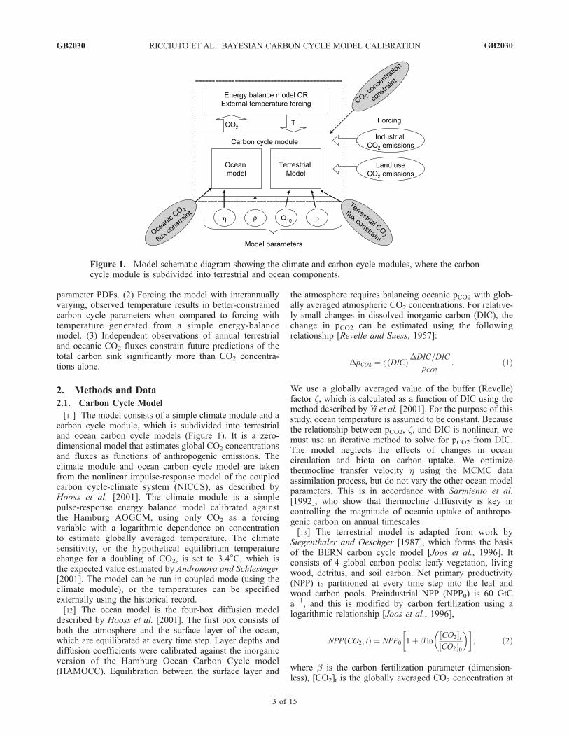
[11] The model consists of a simple climate module and acarbon cycle module, which is subdivided into terrestrialand ocean carbon cycle models (Figure 1). It is a zero-dimensional model that estimates global CO2 concentrationsand fluxes as functions of anthropogenic emissions. Theclimate module and ocean carbon cycle model are takenfrom the nonlinear impulse-response model of the coupledcarbon cycle-climate system (NICCS), as described byHooss et al. [2001]. The climate module is a simplepulse-response energy balance model calibrated againstthe Hamburg AOGCM, using only CO2 as a forcingvariable with a logarithmic dependence on concentrationto estimate globally averaged temperature. The climatesensitivity, or the hypothetical equilibrium temperaturechange for a doubling of CO2, is set to 3.4�C, which isthe expected value estimated by Andronova and Schlesinger[2001]. The model can be run in coupled mode (using theclimate module), or the temperatures can be specifiedexternally using the historical record.[12] The ocean model is the four-box diffusion model

described by Hooss et al. [2001]. The first box consists ofboth the atmosphere and the surface layer of the ocean,which are equilibrated at every time step. Layer depths anddiffusion coefficients were calibrated against the inorganicversion of the Hamburg Ocean Carbon Cycle model(HAMOCC). Equilibration between the surface layer and

the atmosphere requires balancing oceanic pCO2 with glob-ally averaged atmospheric CO2 concentrations. For relative-ly small changes in dissolved inorganic carbon (DIC), thechange in pCO2 can be estimated using the followingrelationship [Revelle and Suess, 1957]:

DpCO2 ¼ z DICð ÞDDIC=DIC

pCO2: ð1Þ

We use a globally averaged value of the buffer (Revelle)factor z, which is calculated as a function of DIC using themethod described by Yi et al. [2001]. For the purpose of thisstudy, ocean temperature is assumed to be constant. Becausethe relationship between pCO2, z, and DIC is nonlinear, wemust use an iterative method to solve for pCO2 from DIC.The model neglects the effects of changes in oceancirculation and biota on carbon uptake. We optimizethermocline transfer velocity h using the MCMC dataassimilation process, but do not vary the other ocean modelparameters. This is in accordance with Sarmiento et al.[1992], who show that thermocline diffusivity is key incontrolling the magnitude of oceanic uptake of anthropo-genic carbon on annual timescales.[13] The terrestrial model is adapted from work by

Siegenthaler and Oeschger [1987], which forms the basisof the BERN carbon cycle model [Joos et al., 1996]. Itconsists of 4 global carbon pools: leafy vegetation, livingwood, detritus, and soil carbon. Net primary productivity(NPP) is partitioned at every time step into the leaf andwood carbon pools. Preindustrial NPP (NPP0) is 60 GtCa�1, and this is modified by carbon fertilization using alogarithmic relationship [Joos et al., 1996],

NPP CO2; tð Þ ¼ NPP0 1þ b lnCO2½ �tCO2½ �0

� �� ; ð2Þ

where b is the carbon fertilization parameter (dimension-less), [CO2]t is the globally averaged CO2 concentration at

Figure 1. Model schematic diagram showing the climate and carbon cycle modules, where the carboncycle module is subdivided into terrestrial and ocean components.


3 of 15

GB2030

time t in parts per million (ppm), and [CO2]0 is thepreindustrial CO2 concentration (280 ppm). For the purposeof this study, we neglect the possible effects of changingmoisture, temperature and radiation on NPP; although thesefactors are important, there is likely to be strong regionalvariation [Nemani et al., 2003], and there are no obviousparameters to describe these effects in a globally aggregatedpredictive model.[14] Given preindustrial conditions, the modeled terrestri-

al carbon cycle is in equilibrium; heterotrophic respirationbalances NPP0, and the net flux from terrestrial ecosystemsto the atmosphere is zero. A portion of the leaf and woodpools are converted to detritus and soil carbon at each timestep, and a portion of detritus is converted to soil carbon.Heterotrophic respiration of CO2 to the atmosphere occursfrom the detritus and soil carbon pools, represented by aloss of a fraction of each pool every time step. Heterotrophicrespiration rates (RH) are modified from preindustrial valuesusing the Q10 relationship,

RH DT ; tð Þ ¼ a1S1 tð Þ þ a2S2 tð Þ½ �QDT10ð Þ

10 ; ð3Þ

where S1 is the size of the detritus pool in GtC, S2 is the sizeof the soil carbon pool in GtC, a1 and a2 are factors relatingthe size of the pool to the annual carbon flux, DT is theglobal temperature deviation from the preindustrial mean(�C), and Q10 is a dimensionless parameter controlling thesensitivity of respiration to temperature. A Q10 of 2, forexample, implies a doubling of global respiration rates for a10�C increase in temperature given a constant carbon poolsize. Note that respiration rates depend not only on Q10 andtemperature at time t, but also on the sizes of the respiringcarbon pools. This results in an increase in respirationthrough the indirect effects of CO2 fertilization, whichcauses the carbon pools to grow larger as a function ofincreasing CO2 concentrations. For simplicity, we assumethat the same Q10 values apply to both the detrital and soilcarbon pools. We also assume that changing values of CO2

and temperature affect neither the partitioning of NPPbetween the leaf and wood pools, nor the partitioning ofcarbon within pools.

2.2. Model Forcing Data

[15] The calibration period of the model is 1850–2004.Future predictions are made using specified emissions orstabilization scenarios from 2005 to 2100. In 1850, terres-trial NPP and pool sizes are set to their preindustrial values[Siegenthaler and Oeschger, 1987], the global temperatureanomaly DT is set to zero, and the atmospheric concentra-tion is set to 280 ppm. The model is then in equilibriumwith no net ocean-atmosphere or net terrestrial-atmospherecarbon fluxes. The model is forced with anthropogenicemissions, including emissions from fossil fuel burning,cement production and land-use change. Global estimates ofcarbon emissions from fossil fuel burning and cementproduction from 1850 to 2002 are from Marland et al.[2005]. We extend this estimate to 2003 and 2004 by linearextrapolation from the previous 10-year period. Land-useemissions from the period 1850–2000 are estimates from

Houghton [2003], with linear extrapolation to 2001–2004from the previous 10-year period. These emissions areexternal to the terrestrial carbon cycle model and do notaffect the terrestrial pool sizes in our simulation. Addition-ally, the model may be forced with a historical temperaturerecord when it is not coupled with the energy balancemodel. In these cases, we use the globally averaged tem-perature data set covering the period from 1856 to 2004from Jones et al. [2005]. We subtract the mean of the periodover the first 30 years of the record, so that the averagetemperature over this period is assumed to equal thepreindustrial mean (where Dt = 0). We also set DT to zeroduring the period 1850–1855, when global temperaturedata were not available. We neglect uncertainties in thetemperature and emissions data.

2.3. Observational Constraints

[16] The model is constrained by observations of CO2

concentrations and estimates of global ocean fluxes. CO2

concentration constraints include data from the Law Domeice core between 1850 and 1959 [Etheridge et al., 1996;MacFarling-Meure et al., 2006], and from the Mauna LoaObservatory from 1960 to 2004 [Keeling and Whorf, 2005].Both sites were chosen as proxies for the global average.The Law Dome data set is an irregular time series in whichdata points represent different samples of air in the ice corewith different ages. We assume that the uncertainty of eachestimate is independent and normally distributed. Thisuncertainty contains both observational error and processerror due to the model structure. The mean air age of thesample was taken as the year of observation for the purposeof model evaluation. The annual Mauna Loa CO2 contains45 annual data points (1960–2004). Because the processerror is not known, we solve for the total uncertainty sm(observational and process error) of these CO2 observationsby including it as a parameter in the data assimilation. In theManua Loa time series, we also account for autocorrelationusing an additional model parameter r. This is discussedfurther below.[17] A number of independent estimates of oceanic sink

strength can be used to constrain our model. The WorldOcean Circulation Experiment (WOCE) in the 1990s in-cluded an extensive survey of DIC and related tracers. Onthe basis of these observations, Sabine et al. [2004],estimate a cumulative oceanic sink for anthropogenic CO2

of 118 ± 19 GtC from 1800 to 1994. Our model assumesthat before 1850, the oceans were in preindustrial equilib-rium; therefore, we take this estimate as a constraint on thecumulative ocean sink from 1850 to 1994. This may be aslight overestimation of uptake because of possible anthro-pogenic emissions that were absorbed before 1850. Asecond constraint on the strength of the oceanic carbonsink arises from the chlorofluorocarbon (CFC) data set,which was combined with measured DIC to estimateaverage annual uptake over the decades of the 1980s andthe 1990s. McNeil et al. [2003] estimate an average annualoceanwide uptake of 1.6 ± 0.4 GtC a�1 over the 1980s, and2.0 ± 0.4 GtC a�1 over the 1990s. To compare the modeloutput to these estimates, modeled annual ocean fluxes wereaveraged over each decade. Because of the limited number


4 of 15

GB2030

of data points, we do not solve for process error orautocorrelation in the oceanic sink observations. The totalerror of these observations is considered to be normallydistributed with a standard deviation equal to the reportedobservational error.

2.4. Data Assimilation Technique

[18] Markov Chain Monte Carlo (MCMC) is a powerfulmethod to assimilate observations into nonlinear modelsthat are relatively fast and have a modest number ofparameters. MCMC simulates direct draws from a jointprobability density function, making no assumptions aboutthe shape of this distribution. We apply MCMC in aBayesian framework by using prior information aboutparameters. We employ the Metropolis-Hastings algorithm[Hastings, 1970; Metropolis et al., 1953].[19] The posterior probability ppost of a sample k from the

joint parameter distribution qqk is a function of the priorprobability pprior and the observations x, and is calculated asfollows:

ppost qkjxð Þ ¼ L xjqkð Þpprior qkð ÞXNi¼1

L xjqið Þpprior qið Þ: ð4Þ

The denominator on the right-hand side of this equation is anormalization factor such that the sum of posterior proba-bilities over N possible sets of parameters is equal to one.The construction of the Markov chain only requires knowl-edge of probability and likelihood ratios, so that we mayignore this normalization factor during this step. Thefunction L is the likelihood of observing all of the obser-vations x given the set of parameters qk. If all observationsare independently and identically distributed (IID) andfollow a normal distribution, then the likelihood is

L xjqkð Þ ¼Yn�1

i¼0

1ffiffiffiffiffiffiffiffiffiffi2ps2

i

p exp � 1

2

f qk; tið Þ � xi

si

� �2 !; ð5Þ

where f(qk, ti) is the model prediction of observation xigiven the set of parameters qk. The likelihood of a set of nindependent observations is the product over the likelihoodsof individual observations x0, x1, . . ., xn�1 at times t0, t1, . . .,tn�1. We assume that each observation is sampled indepen-dently from a normal distribution with a mean xi andstandard deviation si representing the variability due toobservation noise and internal variability that is not cap-tured by the model.[20] This formulation of the likelihood function follows

previous studies using MCMC that assume IID and normallydistributed variability [Braswell et al., 2005;Hargreaves andAnnan, 2002]. This can be a useful and reasonable approx-imation if the observation errors are large and if the processnoise is indeed IID. However, many environmental timeseries show statistically significant autocorrelation. In thiscase, a more refined likelihood function has to be used. Thiscan be illustrated specifically for the annual CO2 concen-trations as observed at Mauna Loa from 1960 to 2004,which display significant autocorrelation as a result of

internal variability that cannot be reproduced by our simplemodel. A different form of the likelihood function is used totest the hypothesis that neglecting autocorrelation in theresiduals (modeled � observed) of annual CO2 concentra-tion causes biased and overconfident parameter estimates.This form does not assume that the residuals are indepen-dent, but instead that they display significant lag-1 autocor-relation. In this case, the model prediction y is given by

yt ¼ f emissions; q; tð Þ: ð6Þ

The variable xt representing observed CO2 concentrations isassumed to be equal to the model prediction yi with asuperimposed error term ui, which is composed of a randomcomponent and a component that depends upon theprevious time step,

xt ¼ f emissions; q; tð Þ þ ut

ut ¼ rut�1 þ et:ð7Þ

The et term represents the total error term, which is assumedto be independent and normally distributed with a mean ofzero and a standard deviation s. The term ut is assumed tobe generated by a first-order autoregressive process. Giventhese assumptions, the likelihood function is given byZellner and Tiao [1964],

L xjqkð Þ ¼ 1

sffiffiffiffiffiffi2p

p� �n

exp � f qk ; t0ð Þ � x0 �Mð Þ2

2s2

(

�Xn�1

i¼1

f qk ; tið Þ � xi � r f qk; ti�1ð Þ � xi�1ð Þð Þ2

2s2

)ð8Þ

This represents the likelihood of observing x, which is avector of observations with n time steps, given a set ofparameters qk. r is the lag-1 autocorrelation parameter, forwhich we estimate the PDF in the same manner as thecarbon cycle parameters. These assumptions also requirethat the uncertainty in the mean of the observation for thefirst time step (t = 0) be specified as an unknown parameterM. Because the effect of this parameter is small, we neglectit in this analysis to improve computational efficiency.Neglecting this parameter is equivalent to considering theconditional likelihood. Unlike equation (5), this form ofthe likelihood function assumes that all observations havethe same standard deviation of total error s.[21] To construct the joint parameter PDF, we must

sample many sets of parameters q. In a Bayesian frame-work, prior information is combined with the likelihood toproduce a posterior probability using equation (4). Thesimplest way to do this would be to compute likelihoodsat random points over the range of the prior distribution andcombine this information to produce a PDF. However, mostof the posterior probability mass may be concentrated in asmall area of the prior range, making this sampling methodinefficient. MCMC makes use of information about theshape of the likelihood function in order to preferentiallysample in regions where the posterior probability is high.


5 of 15

GB2030

This technique is best suited for convex problems with asingle maximum of the likelihood function.[22] After a sufficiently long iteration (referred to as the

‘‘burn-in’’ period), the Markov chain reaches a stationarydistribution that converges to the joint parameter posteriorPDF. A length of 106 model evaluations with a burn-inperiod of 105 evaluations results in numerically stableresults for the considered problem. We choose proposalstep sizes that result in acceptance rates between 25 and50%, which is generally the most efficient range for theMCMC algorithm [Harmon and Challenor, 1997]. Afterburn-in values are removed, this yields a Markov chainlength of at least 2 105 parameter sets that are used toconstruct parameter estimates and uncertainties. This valueis considerably lower than the total number of modelevaluations because many proposal steps are not accepted.A comparison among multiple chains with different startingpoints indicates that a length of 2 105 is sufficient toconverge to the joint posterior PDFs at the resolution thatthey are presented.[23] Initial carbon cycle parameters are chosen from the

best estimates in the literature, and the value of the lag-1autocorrelation r is set to 0 in accordance with the nullhypothesis that there is no autocorrelation in the residuals ofannual CO2 concentration data (Table 1). Parameter priordistributions are nearly uninformative (uniformly distribu-ted over a large range) where possible, but nonphysicalvalues of parameters are excluded. The thermocline transfervelocity h prior ranges from 0 to 1000 m a�1 to excludenegative values, which are nonphysical. The carbon fertiliza-tion parameter b ranges from 0 to 1000; the exclusion ofnegative values in this case means that increased atmosphericCO2 concentrations cannot decrease NPP. Similarly, Q10

ranges from 1 to 1000 so that increased temperaturemust havethe effect of increasing respiration. The upper limit of 1000 forall three of these parameters is an arbitrary value chosen to belarge enough that our finite Markov chains are never actuallyconstrained by these bounds. The lag 1 autocorrelationparameter r is a correlation coefficient and ranges between�1and 1. The parameter sm, the standard deviation of theManua Loa CO2 residuals, ranges from 0.1 (the estimatedobservation error) to 10.0 ppm.

2.5. Experimental Design

[24] To test the first two hypotheses outlined above, threeseparate model calibrations are performed: (case a) basecase, with observed interannually varying temperature andaccounting for autocorrelation in the likelihood function asin equation (8); (case b) neglecting autocorrelation, withobserved temperature and neglecting autocorrelation in thelikelihood function as in equation (5); and (case c) smooth

temperature, with modeled (smooth) temperature and ac-counting for autocorrelation in the likelihood function. Allassimilations use the same number of model evaluations,initial guesses, step sizes and prior distributions for modelparameters except that in the second experiment, the auto-correlation parameter r is held constant at zero. Three sets ofjoint parameter PDFs are then obtained. A comparisonbetween calibrations a and b is used to test the first hypothesisthat neglecting autocorrelation results in biased and over-confident parameter estimates. A comparison betweencalibrations a and c is used to test the second hypothesisthat forcing the model with observed temperature is avaluable constraint on the terrestrial carbon cycle parameters.[25] The Markov chain generated from base case is used

for predictions and additional analysis. We predict themagnitude of the allowable CO2 emissions through the year2100 under the S550 ppm IPCC stabilization scenario fromthe years 2005–2100. Using a fixed concentration ratherthan anthropogenic emissions as input requires a slightlydifferent model construction. For each year, the temperaturedeviation DT is calculated given the specified CO2 concen-tration, and the strength of the carbon sink is then estimatedgiven the model parameters, CO2 concentration, DT, and aninitial estimate of allowable emissions. The quantity ‘‘al-lowable emissions’’ is defined as the amount of anthropo-genic emissions (land use + fossil fuel) necessary to stay onthe stabilization scenario concentration trajectory, given thestrength of the carbon sink. Because anthropogenic emis-sions are a model input and CO2 concentrations are a modeloutput, we use an iterative process to equilibrate prescribedCO2 concentrations with allowable emissions.[26] Finally, we test the hypothesis that observations of

annual terrestrial and oceanic CO2 fluxes reduce totalpredicted sink uncertainty, which is equivalent to theuncertainty in allowable emissions in the stabilizationscenario. These flux ‘‘observations’’ are generated fromthe base-case maximum likelihood solution, and observa-tion error is superimposed on these values. We neglectpossible process error, which is unknown because actualobservations do not exist. Future ‘‘observations’’ of CO2 arealso generated from the base-case maximum likelihoodsolution. We simulate the effects of observation and processerror seen in the Mauna Loa observations by superimposingan AR1 process on these observations. The AR1 process isgenerated using the maximum likelihood value of the lag-1autocorrelation parameter r and the standard deviation ofthe total error s. In addition, we generate a temperature timeseries for use in the model. The long-term trend is predictedusing the simple energy-balance model, and an AR1 processis superimposed on this time series with the same statisticalproperties as the 1856–2004 observations. To reduce noise

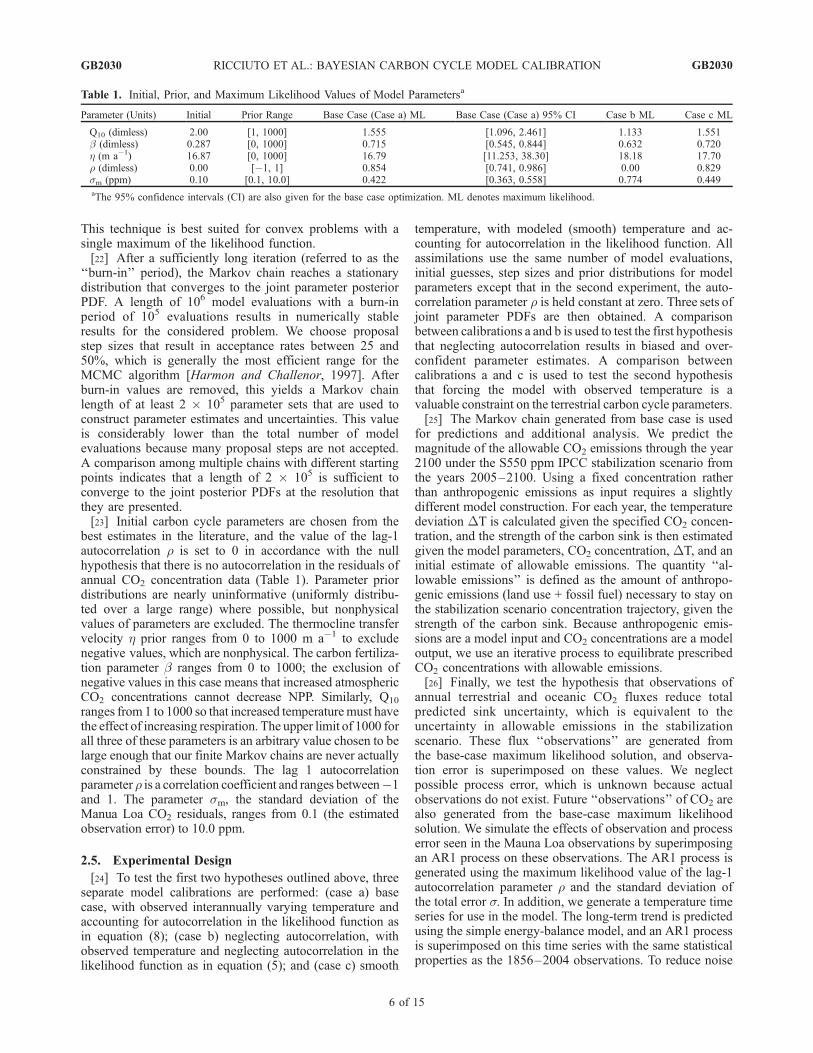
Table 1. Initial, Prior, and Maximum Likelihood Values of Model Parametersa

Parameter (Units) Initial Prior Range Base Case (Case a) ML Base Case (Case a) 95% CI Case b ML Case c ML

Q10 (dimless) 2.00 [1, 1000] 1.555 [1.096, 2.461] 1.133 1.551b (dimless) 0.287 [0, 1000] 0.715 [0.545, 0.844] 0.632 0.720h (m a�1) 16.87 [0, 1000] 16.79 [11.253, 38.30] 18.18 17.70r (dimless) 0.00 [�1, 1] 0.854 [0.741, 0.986] 0.00 0.829sm (ppm) 0.10 [0.1, 10.0] 0.422 [0.363, 0.558] 0.774 0.449

aThe 95% confidence intervals (CI) are also given for the base case optimization. ML denotes maximum likelihood.


6 of 15

GB2030

in predictions of allowable emissions uncertainty, wegenerate ten AR1 time series with the same statisticalproperties to produce different realizations of the predictedtemperature and CO2 time series; results are averaged.[27] Specifically, we test four cases: (1) no observations

of terrestrial or oceanic fluxes, and annual observations ofterrestrial and oceanic fluxes with uncertainties of (2) 1.00GtC a�1, (3) 0.50 GtC a�1 and (4) 0.25 GtC a�1. In all fourcases, we assume that CO2 concentrations are still observedannually at Mauna Loa. We then examine the 95% range ofallowable emissions in the year 2050 as a function ofnumber of annual observations beginning in 2005 and asa function of observational uncertainty.

3. Results and Discussion

3.1. Base-Case Parameter Distributions

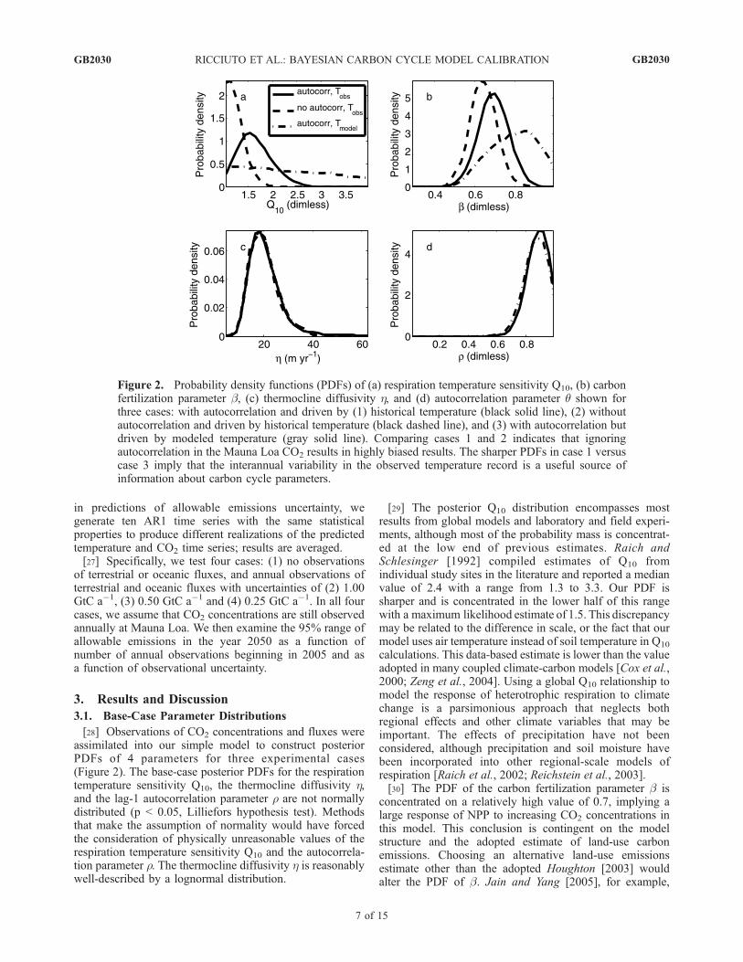
[28] Observations of CO2 concentrations and fluxes wereassimilated into our simple model to construct posteriorPDFs of 4 parameters for three experimental cases(Figure 2). The base-case posterior PDFs for the respirationtemperature sensitivity Q10, the thermocline diffusivity h,and the lag-1 autocorrelation parameter r are not normallydistributed (p < 0.05, Lilliefors hypothesis test). Methodsthat make the assumption of normality would have forcedthe consideration of physically unreasonable values of therespiration temperature sensitivity Q10 and the autocorrela-tion parameter r. The thermocline diffusivity h is reasonablywell-described by a lognormal distribution.

[29] The posterior Q10 distribution encompasses mostresults from global models and laboratory and field experi-ments, although most of the probability mass is concentrat-ed at the low end of previous estimates. Raich andSchlesinger [1992] compiled estimates of Q10 fromindividual study sites in the literature and reported a medianvalue of 2.4 with a range from 1.3 to 3.3. Our PDF issharper and is concentrated in the lower half of this rangewith a maximum likelihood estimate of 1.5. This discrepancymay be related to the difference in scale, or the fact that ourmodel uses air temperature instead of soil temperature in Q10

calculations. This data-based estimate is lower than the valueadopted in many coupled climate-carbon models [Cox et al.,2000; Zeng et al., 2004]. Using a global Q10 relationship tomodel the response of heterotrophic respiration to climatechange is a parsimonious approach that neglects bothregional effects and other climate variables that may beimportant. The effects of precipitation have not beenconsidered, although precipitation and soil moisture havebeen incorporated into other regional-scale models ofrespiration [Raich et al., 2002; Reichstein et al., 2003].[30] The PDF of the carbon fertilization parameter b is

concentrated on a relatively high value of 0.7, implying alarge response of NPP to increasing CO2 concentrations inthis model. This conclusion is contingent on the modelstructure and the adopted estimate of land-use carbonemissions. Choosing an alternative land-use emissionsestimate other than the adopted Houghton [2003] wouldalter the PDF of b. Jain and Yang [2005], for example,

Figure 2. Probability density functions (PDFs) of (a) respiration temperature sensitivity Q10, (b) carbonfertilization parameter b, (c) thermocline diffusivity h, and (d) autocorrelation parameter q shown forthree cases: with autocorrelation and driven by (1) historical temperature (black solid line), (2) withoutautocorrelation and driven by historical temperature (black dashed line), and (3) with autocorrelation butdriven by modeled temperature (gray solid line). Comparing cases 1 and 2 indicates that ignoringautocorrelation in the Mauna Loa CO2 results in highly biased results. The sharper PDFs in case 1 versuscase 3 imply that the interannual variability in the observed temperature record is a useful source ofinformation about carbon cycle parameters.


7 of 15

GB2030

conclude that land-use emissions estimates derived fromHoughton [2003] are considerably larger than their modeledestimate based on the land-use data set of Ramankutty andFoley [1999]. Different ecosystem models produce asignificant spread in estimates of land-use emissions evenwhen forced with the same land-use change data set[McGuire et al., 2001]. Because the oceanic sink isconstrained, a land-use emission uncertainty would translateinto increased uncertainty about the terrestrial carbon cycleparameters, especially b.[31] In the Bern carbon cycle model, which forms the

basis for our terrestrial model and uses the same formulationfor carbon fertilization, a value of b = 0.287 was used tobalance an estimated deforestation source of 1.1 GtC a�1 inthe 1980s. [Joos et al., 1996]. The maximum likelihoodestimate of b (Figure 2) is more than twice this value, butwithin the upper range of values in other models[Kicklighter et al., 1999]. This difference from the Bernmodel is primarily driven by the fact that Houghton [2003]estimates a larger anthropogenic land-use emission flux ofnearly 2.0 GtC a�1 in the 1980s. In addition, our modelrequires a larger value of b to balance the respirationincrease resulting from increased temperature, which is notconsidered in the Bern model [Joos et al., 1996]. Our valueof b = 0.7 implies that NPP has increased by 12 GtC a�1

(20%) since preindustrial times. Despite the discrepancybetween this and other models, the estimated PDF of b isconsistent with free-air carbon enrichment (FACE) experi-mental data, which indicate a value of b = 0.6 across a rangeof diverse sites [Norby et al., 2005].[32] The global aggregate modeling approach allows for a

rigorous statistical analysis with small computationaldemands but limits the number of considered processes.Changes in regional temperatures, precipitation patterns andnitrogen fertilization may be important drivers of theterrestrial carbon sink. For example, Bruno and Joos[1997] conclude that carbon fertilization is insufficient toexplain the biospheric sink. Caspersen et al. [2000] estimatethat growth enhancement due to carbon fertilization isnegligible in the upper Midwest region of the United States,and that forest regrowth is the primary reason for the carbonsink in this region. However, this may not be true of allregions, and the forest inventory data used in this analysismay lack the precision necessary to make the conclusionthat carbon fertilization is negligible [Joos et al., 2002].[33] The mode of the estimated thermocline transfer

velocity h is approximately 16.8 m a�1, nearly identical tothe 16.9 m a�1 used in the original version of NICCS thatwas calibrated against the Hamburg Ocean Carbon Cyclemodel [Hooss et al., 2001]. There is a wide distribution ofvalues, as the 95% confidence interval ranges from 11.25 ma�1 to 38.3 m a�1. This implies a large uncertainty in thestrength of the ocean carbon sink despite the observationalconstraints. Note that within the adopted model structure,the observational constraints of Sabine et al. [2004] andMcNeil et al. [2003] slightly contradict each other, whichmagnifies the uncertainty associated with the ocean carbonsink (discussed below).[34] The assimilation produces significant correlations

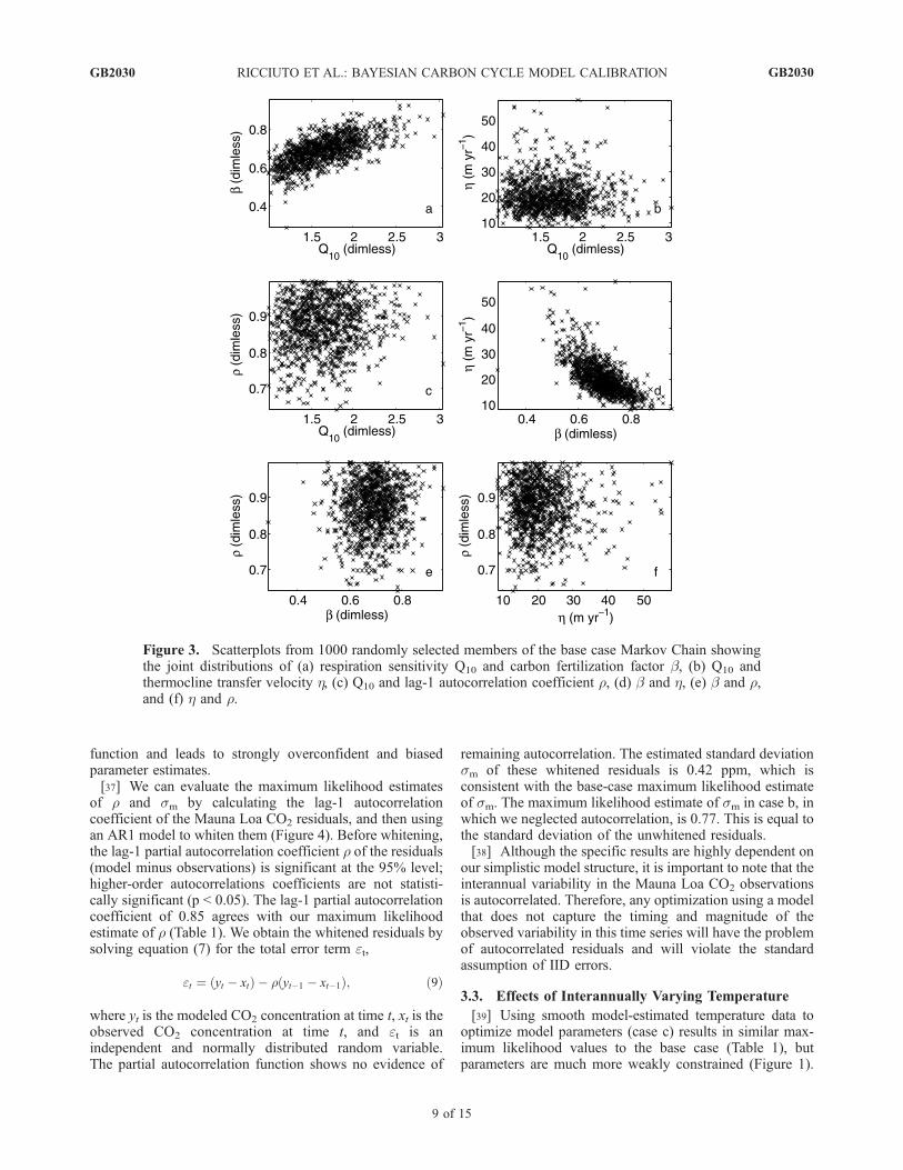
(p < 0.05) in two pairs of model parameters (Figure 3).

There is a significant positive correlation between (1) therespiration temperature sensitivity (Q10) and the carbonfertilization parameter (b) and (2) the carbon fertilizationparameter (b) and the thermocline transfer velocity (h). Asdiscussed above, the atmospheric CO2 budget provides astrong constraint on the total sink strength but a poorconstraint on the partitioning between the terrestrial andocean sinks. The considered ocean sink observationsconstrain the terrestrial sink, because the total sink is givenby the atmospheric CO2 budget. Uncertainty in theobservational constraints on the ocean sink hence directlytranslates into uncertainty in the partitioning of the terrestrialand ocean carbon sinks. As a result, the carbon fertilizationfactor (b) is positively correlated with the strength of theterrestrial sink, and the thermocline transfer velocity (h) ispositively correlated with the strength of the ocean carbonsink. The inverse correlation between the carbon fertilizationfactor b and the thermocline diffusivity h results because highvalues of the carbon fertilization factor and low values ofthermocline diffusivity match the observational constraints ina similar way as low values of the carbon fertilization factorand high values of thermocline transfer velocity.[35] Our analysis does not consider constraints on terres-

trial gross fluxes (NPP and respiration) as the only obser-vationally based candidates are the results of inversions ofCO2 concentrations or derived from other tracers that wehave not included in our model for simplicity. Because weuse global CO2 as a constraint, synthesis inversions usingCO2 concentrations are not independent sources of infor-mation unless trend information is removed, which is nottypically done and removes most of the information fromthe inversion [Enting, 2002]. A calibration including globalterrestrial carbon uptake (similar to the oceanic constraints)would likely result in a stronger constraint on carbon fluxpartitioning. The observed positive correlation betweenrespiration temperature sensitivity (Q10) and the carbonfertilization factor (b) is expected because the carbonfertilization factor controls the magnitude of NPP and therespiration temperature sensitivity Q10 controls the magni-tude of respiration. High values of respiration and highvalues of NPP produce a similar net terrestrial sink as lowvalues of respiration and low values of NPP. Our analysissuggests no significant correlation (p < 0.05) betweenrespiration temperature sensitivity (Q10) and thermoclinetransfer velocity (h), or between the lag-1 autocorrelationparameter (r) and any of the other three parameters.

3.2. Effects of Neglecting Autocorrelation

[36] Neglecting autocorrelation in the likelihood functionchanges the character of parameter PDFs (Figure 1).Neglecting autocorrelation biases the mode of the posteriorQ10 value by about 30% and results in an arepsicialtightening of the 95% confidence limit by about 50%.Similarly, the carbon fertilization factor b is shifted towardlower values with a maximum likelihood estimate that is10% lower and a 95% confidence interval that is 15%tighter when neglecting autocorrelation. The estimate of h isless affected. Neglecting autocorrelation violates an im-portant assumption used in constructing the likelihood


8 of 15

GB2030

function and leads to strongly overconfident and biasedparameter estimates.[37] We can evaluate the maximum likelihood estimates

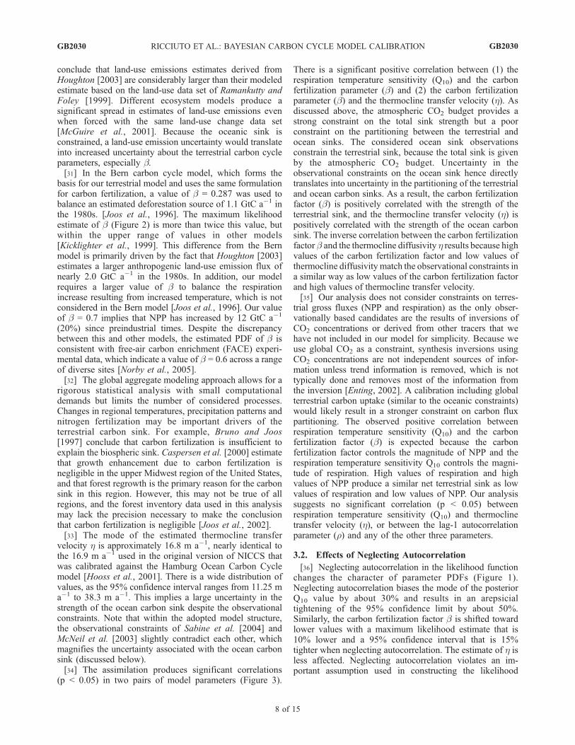
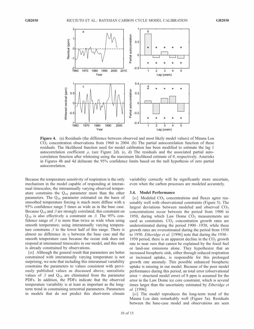
of r and sm by calculating the lag-1 autocorrelationcoefficient of the Mauna Loa CO2 residuals, and then usingan AR1 model to whiten them (Figure 4). Before whitening,the lag-1 partial autocorrelation coefficient r of the residuals(model minus observations) is significant at the 95% level;higher-order autocorrelations coefficients are not statisti-cally significant (p < 0.05). The lag-1 partial autocorrelationcoefficient of 0.85 agrees with our maximum likelihoodestimate of r (Table 1). We obtain the whitened residuals bysolving equation (7) for the total error term et,

et ¼ yt � xtð Þ � r yt�1 � xt�1ð Þ; ð9Þ

where yt is the modeled CO2 concentration at time t, xt is theobserved CO2 concentration at time t, and et is anindependent and normally distributed random variable.The partial autocorrelation function shows no evidence of

remaining autocorrelation. The estimated standard deviationsm of these whitened residuals is 0.42 ppm, which isconsistent with the base-case maximum likelihood estimateof sm. The maximum likelihood estimate of sm in case b, inwhich we neglected autocorrelation, is 0.77. This is equal tothe standard deviation of the unwhitened residuals.[38] Although the specific results are highly dependent on

our simplistic model structure, it is important to note that theinterannual variability in the Mauna Loa CO2 observationsis autocorrelated. Therefore, any optimization using a modelthat does not capture the timing and magnitude of theobserved variability in this time series will have the problemof autocorrelated residuals and will violate the standardassumption of IID errors.

3.3. Effects of Interannually Varying Temperature

[39] Using smooth model-estimated temperature data tooptimize model parameters (case c) results in similar max-imum likelihood values to the base case (Table 1), butparameters are much more weakly constrained (Figure 1).

Figure 3. Scatterplots from 1000 randomly selected members of the base case Markov Chain showingthe joint distributions of (a) respiration sensitivity Q10 and carbon fertilization factor b, (b) Q10 andthermocline transfer velocity h, (c) Q10 and lag-1 autocorrelation coefficient r, (d) b and h, (e) b and r,and (f) h and r.


9 of 15

GB2030

Because the temperature sensitivity of respiration is the onlymechanism in the model capable of responding at interan-nual timescales, the interannually varying observed temper-ature constrains the Q10 parameter more than the otherparameters. The Q10 parameter estimated on the basis ofsmoothed temperature forcing is much more diffuse with a95% confidence range 5 times as wide as in the base case.Because Q10 and b are strongly correlated, this constraint onQ10 is also effectively a constraint on b. The 95% con-fidence range of b is more than twice as wide when usingsmooth temperature; using interannually varying tempera-ture constrains b to the lower half of this range. There isalmost no difference in h between the base case and thesmooth temperature case because the ocean sink does notrespond at interannual timescales in our model, and this sinkis already constrained by observations.[40] Although the general result that parameters are better

constrained with interannually varying temperature is notsurprising, we note that including this interannual variabilityconstrains the parameters to values consistent with previ-ously published values as discussed above; unrealisticvalues of b and Q10 are eliminated from the parameterPDFs. In addition, the PDFs indicate that the observedtemperature variability is at least as important as the long-term trend in constraining terrestrial parameters. Parametersin models that do not predict this short-term climate

variability correctly will be significantly more uncertain,even when the carbon processes are modeled accurately.

3.4. Model Performance

[41] Modeled CO2 concentrations and fluxes agree rea-sonably well with observational constraints (Figure 5). Thelargest deviations between modeled and observed CO2

concentrations occur between the period from 1900 to1950, during which Law Dome CO2 measurements areused as constraints. CO2 concentration growth rates areunderestimated during the period 1900–1930, while thesegrowth rates are overestimated during the period from 1930to 1950. Etheridge et al. [1996] note that during the 1930–1950 period, there is an apparent decline in the CO2 growthrate to near zero that cannot be explained by the fossil fuelor land-use emissions alone. They hypothesize that anincreased biospheric sink, either through reduced respirationor increased uptake, is responsible for this prolongedgrowth rate anomaly. This possible enhanced biosphericuptake is missing in our model. Because of the poor modelperformance during this period, an total error (observationalerror + structural model error) of 8 ppm is assumed for theerror in the Law Dome ice core constraint, which is severaltimes larger than the uncertainty estimated by Etheridge etal. [1996].[42] The model reproduces the long-term trend of the

Mauna Loa data remarkably well (Figure 5a). Residualsbetween the base-case model and observations are seen

Figure 4. (a) Residuals (the difference between observed and most likely model values) of Mauna LoaCO2 concentration observations from 1960 to 2004. (b) The partial autocorrelation function of theseresiduals. The likelihood function used for model calibration has been modified to estimate the lag 1autocorrelation coefficient r, (see Figure 2d). (c, d) The residuals and the associated partial auto-correlation function after whitening using the maximum likelihood estimate of q, respectively. Asterisksin Figures 4b and 4d delineate the 95% confidence limits based on the null hypothesis of zero partialautocorrelation.


10 of 15

GB2030

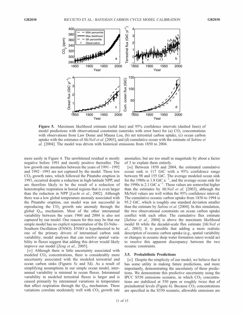
more easily in Figure 4. The unwhitened residual is mostlynegative before 1991 and mostly positive thereafter. Thelow growth rate anomalies between the years of 1991–1992and 1992–1993 are not captured by the model. These lowCO2 growth rates, which followed the Pinatubo eruption in1991, occurred despite a reduction in high-latitude NPP, andare therefore likely to be the result of a reduction ofheterotrophic respiration in boreal regions that is even largerthan the reduction in NPP [Lucht et al., 2002]. Althoughthere was a low global temperature anomaly associated withthe Pinatubo eruption, our model was not successful inreproducing the CO2 growth rate anomaly through theglobal Q10 mechanism. Most of the other interannualvariability between the years 1960 and 2004 is also notcaptured by our model. One reason for this may be that oursimple model has no explicit representation of the El-Nino–Southern Oscillation (ENSO). ENSO is hypothesized to beone of the primary drivers of interannual carbon sinkvariability; model analyses that can resolve spatial varia-bility in fluxes suggest that adding this driver would likelyimprove our model [Zeng et al., 2005].[43] Although there is little uncertainty associated with

modeled CO2 concentrations, there is considerably moreuncertainty associated with the modeled terrestrial andocean carbon sinks (Figures 5c and 5d). As a result ofsimplifying assumptions in our simple ocean model, inter-annual variability is minimal in ocean fluxes. Interannualvariability in modeled terrestrial fluxes is larger and iscaused primarily by interannual variations in temperaturethat affect respiration through the Q10 mechanism. Thesevariations correlate moderately well with CO2 growth rate

anomalies, but are too small in magnitude by about a factorof 3 to explain them entirely.[44] Between 1850 and 2004, the estimated cumulative

ocean sink is 117 GtC with a 95% confidence rangebetween 98 and 155 GtC. The average modeled ocean sinkfor the 1980s is 1.8 GtC a�1, and the average ocean sink forthe 1990s is 2.1 GtC a�1. These values are somewhat higherthan the estimates by McNeil et al. [2003], although theMcNeil values are well within the 95% confidence interval.The cumulative oceanic carbon uptake from 1850 to 1994 is95.2 GtC, which is roughly one standard deviation smallerthan the estimate by Sabine et al. [2004]. In this simulation,the two observational constraints on ocean carbon uptakeconflict with each other. The cumulative flux estimate[Sabine et al., 2004] is above the maximum likelihoodmodel fit while the decadal-scale flux estimate [McNeil etal., 2003]. It is possible that adding a more realisticdescription of oceanic carbon uptake (e.g., spatial variabilityor changes in oceanic deep water formation rates) would actto resolve this apparent discrepancy between the twooceanic constraints.

3.5. Probabilistic Predictions

[45] Despite the simplicity of our model, we believe that ithas some utility in making future predictions, and moreimportantly, demonstrating the uncertainty of these predic-tions. We demonstrate this predictive uncertainty using theIPCC S550 emissions scenario, in which CO2 concentra-tions are stabilized at 550 ppm or roughly twice that ofpreindustrial levels (Figure 6). Because CO2 concentrationsare specified in the S550 scenario, allowable emissions are

Figure 5. Maximum likelihood estimate (solid line) and 95% confidence intervals (dashed lines) ofmodel predictions with observational constraints (asterisks with error bars) for (a) CO2 concentrationswith observations from Law Dome and Mauna Loa, (b) net terrestrial carbon uptake, (c) ocean carbonuptake with the estimates ofMcNeil et al. [2003], and (d) cumulative ocean with the estimate of Sabine etal. [2004]. The model was driven with historical emissions from 1850 to 2004.


11 of 15

GB2030

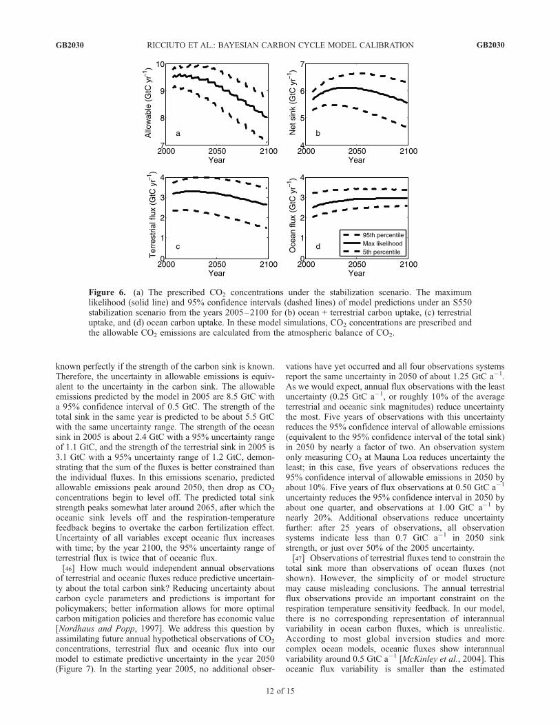
known perfectly if the strength of the carbon sink is known.Therefore, the uncertainty in allowable emissions is equiv-alent to the uncertainty in the carbon sink. The allowableemissions predicted by the model in 2005 are 8.5 GtC witha 95% confidence interval of 0.5 GtC. The strength of thetotal sink in the same year is predicted to be about 5.5 GtCwith the same uncertainty range. The strength of the oceansink in 2005 is about 2.4 GtC with a 95% uncertainty rangeof 1.1 GtC, and the strength of the terrestrial sink in 2005 is3.1 GtC with a 95% uncertainty range of 1.2 GtC, demon-strating that the sum of the fluxes is better constrained thanthe individual fluxes. In this emissions scenario, predictedallowable emissions peak around 2050, then drop as CO2

concentrations begin to level off. The predicted total sinkstrength peaks somewhat later around 2065, after which theoceanic sink levels off and the respiration-temperaturefeedback begins to overtake the carbon fertilization effect.Uncertainty of all variables except oceanic flux increaseswith time; by the year 2100, the 95% uncertainty range ofterrestrial flux is twice that of oceanic flux.[46] How much would independent annual observations

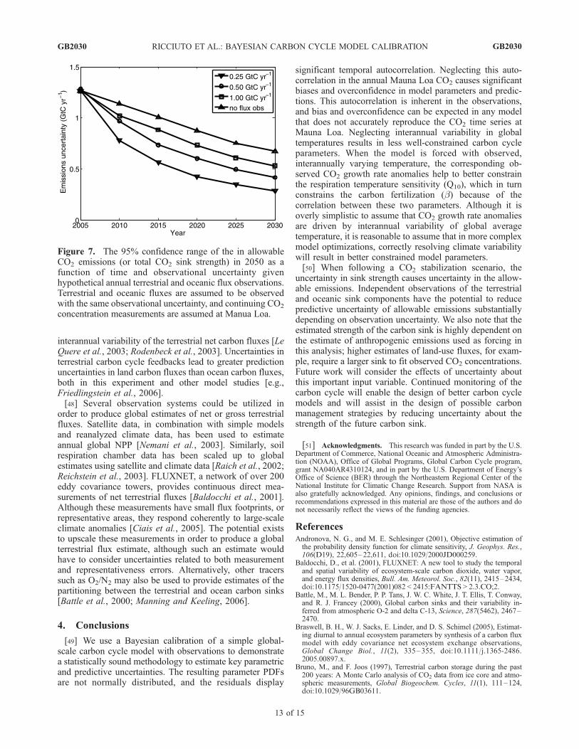
of terrestrial and oceanic fluxes reduce predictive uncertain-ty about the total carbon sink? Reducing uncertainty aboutcarbon cycle parameters and predictions is important forpolicymakers; better information allows for more optimalcarbon mitigation policies and therefore has economic value[Nordhaus and Popp, 1997]. We address this question byassimilating future annual hypothetical observations of CO2

concentrations, terrestrial flux and oceanic flux into ourmodel to estimate predictive uncertainty in the year 2050(Figure 7). In the starting year 2005, no additional obser-

vations have yet occurred and all four observations systemsreport the same uncertainty in 2050 of about 1.25 GtC a�1.As we would expect, annual flux observations with the leastuncertainty (0.25 GtC a�1, or roughly 10% of the averageterrestrial and oceanic sink magnitudes) reduce uncertaintythe most. Five years of observations with this uncertaintyreduces the 95% confidence interval of allowable emissions(equivalent to the 95% confidence interval of the total sink)in 2050 by nearly a factor of two. An observation systemonly measuring CO2 at Mauna Loa reduces uncertainty theleast; in this case, five years of observations reduces the95% confidence interval of allowable emissions in 2050 byabout 10%. Five years of flux observations at 0.50 GtC a�1

uncertainty reduces the 95% confidence interval in 2050 byabout one quarter, and observations at 1.00 GtC a�1 bynearly 20%. Additional observations reduce uncertaintyfurther: after 25 years of observations, all observationsystems indicate less than 0.7 GtC a�1 in 2050 sinkstrength, or just over 50% of the 2005 uncertainty.[47] Observations of terrestrial fluxes tend to constrain the

total sink more than observations of ocean fluxes (notshown). However, the simplicity of or model structuremay cause misleading conclusions. The annual terrestrialflux observations provide an important constraint on therespiration temperature sensitivity feedback. In our model,there is no corresponding representation of interannualvariability in ocean carbon fluxes, which is unrealistic.According to most global inversion studies and morecomplex ocean models, oceanic fluxes show interannualvariability around 0.5 GtC a�1 [McKinley et al., 2004]. Thisoceanic flux variability is smaller than the estimated

Figure 6. (a) The prescribed CO2 concentrations under the stabilization scenario. The maximumlikelihood (solid line) and 95% confidence intervals (dashed lines) of model predictions under an S550stabilization scenario from the years 2005–2100 for (b) ocean + terrestrial carbon uptake, (c) terrestrialuptake, and (d) ocean carbon uptake. In these model simulations, CO2 concentrations are prescribed andthe allowable CO2 emissions are calculated from the atmospheric balance of CO2.


12 of 15

GB2030

interannual variability of the terrestrial net carbon fluxes [LeQuere et al., 2003; Rodenbeck et al., 2003]. Uncertainties interrestrial carbon cycle feedbacks lead to greater predictionuncertainties in land carbon fluxes than ocean carbon fluxes,both in this experiment and other model studies [e.g.,Friedlingstein et al., 2006].[48] Several observation systems could be utilized in

order to produce global estimates of net or gross terrestrialfluxes. Satellite data, in combination with simple modelsand reanalyzed climate data, has been used to estimateannual global NPP [Nemani et al., 2003]. Similarly, soilrespiration chamber data has been scaled up to globalestimates using satellite and climate data [Raich et al., 2002;Reichstein et al., 2003]. FLUXNET, a network of over 200eddy covariance towers, provides continuous direct mea-surements of net terrestrial fluxes [Baldocchi et al., 2001].Although these measurements have small flux footprints, orrepresentative areas, they respond coherently to large-scaleclimate anomalies [Ciais et al., 2005]. The potential existsto upscale these measurements in order to produce a globalterrestrial flux estimate, although such an estimate wouldhave to consider uncertainties related to both measurementand representativeness errors. Alternatively, other tracerssuch as O2/N2 may also be used to provide estimates of thepartitioning between the terrestrial and ocean carbon sinks[Battle et al., 2000; Manning and Keeling, 2006].

4. Conclusions

[49] We use a Bayesian calibration of a simple global-scale carbon cycle model with observations to demonstratea statistically sound methodology to estimate key parametricand predictive uncertainties. The resulting parameter PDFsare not normally distributed, and the residuals display

significant temporal autocorrelation. Neglecting this auto-correlation in the annual Mauna Loa CO2 causes significantbiases and overconfidence in model parameters and predic-tions. This autocorrelation is inherent in the observations,and bias and overconfidence can be expected in any modelthat does not accurately reproduce the CO2 time series atMauna Loa. Neglecting interannual variability in globaltemperatures results in less well-constrained carbon cycleparameters. When the model is forced with observed,interannually varying temperature, the corresponding ob-served CO2 growth rate anomalies help to better constrainthe respiration temperature sensitivity (Q10), which in turnconstrains the carbon fertilization (b) because of thecorrelation between these two parameters. Although it isoverly simplistic to assume that CO2 growth rate anomaliesare driven by interannual variability of global averagetemperature, it is reasonable to assume that in more complexmodel optimizations, correctly resolving climate variabilitywill result in better constrained model parameters.[50] When following a CO2 stabilization scenario, the

uncertainty in sink strength causes uncertainty in the allow-able emissions. Independent observations of the terrestrialand oceanic sink components have the potential to reducepredictive uncertainty of allowable emissions substantiallydepending on observation uncertainty. We also note that theestimated strength of the carbon sink is highly dependent onthe estimate of anthropogenic emissions used as forcing inthis analysis; higher estimates of land-use fluxes, for exam-ple, require a larger sink to fit observed CO2 concentrations.Future work will consider the effects of uncertainty aboutthis important input variable. Continued monitoring of thecarbon cycle will enable the design of better carbon cyclemodels and will assist in the design of possible carbonmanagement strategies by reducing uncertainty about thestrength of the future carbon sink.

[51] Acknowledgments. This research was funded in part by the U.S.Department of Commerce, National Oceanic and Atmospheric Administra-tion (NOAA), Office of Global Programs, Global Carbon Cycle program,grant NA040AR4310124, and in part by the U.S. Department of Energy’sOffice of Science (BER) through the Northeastern Regional Center of theNational Institute for Climatic Change Research. Support from NASA isalso gratefully acknowledged. Any opinions, findings, and conclusions orrecommendations expressed in this material are those of the authors and donot necessarily reflect the views of the funding agencies.

ReferencesAndronova, N. G., and M. E. Schlesinger (2001), Objective estimation ofthe probability density function for climate sensitivity, J. Geophys. Res.,106(D19), 22,605–22,611, doi:10.1029/2000JD000259.

Baldocchi, D., et al. (2001), FLUXNET: A new tool to study the temporaland spatial variability of ecosystem-scale carbon dioxide, water vapor,and energy flux densities, Bull. Am. Meteorol. Soc., 82(11), 2415–2434,doi:10.1175/1520-0477(2001)082<2415:FANTTS>2.3.CO;2.

Battle, M., M. L. Bender, P. P. Tans, J. W. C. White, J. T. Ellis, T. Conway,and R. J. Francey (2000), Global carbon sinks and their variability in-ferred from atmospheric O-2 and delta C-13, Science, 287(5462), 2467–2470.

Braswell, B. H., W. J. Sacks, E. Linder, and D. S. Schimel (2005), Estimat-ing diurnal to annual ecosystem parameters by synthesis of a carbon fluxmodel with eddy covariance net ecosystem exchange observations,Global Change Biol., 11(2), 335–355, doi:10.1111/j.1365-2486.2005.00897.x.

Bruno, M., and F. Joos (1997), Terrestrial carbon storage during the past200 years: A Monte Carlo analysis of CO2 data from ice core and atmo-spheric measurements, Global Biogeochem. Cycles, 11(1), 111–124,doi:10.1029/96GB03611.

Figure 7. The 95% confidence range of the in allowableCO2 emissions (or total CO2 sink strength) in 2050 as afunction of time and observational uncertainty givenhypothetical annual terrestrial and oceanic flux observations.Terrestrial and oceanic fluxes are assumed to be observedwith the same observational uncertainty, and continuing CO2

concentration measurements are assumed at Manua Loa.


13 of 15

GB2030

Caspersen, J. P., S. W. Pacala, J. C. Jenkins, G. C. Hurtt, P. R. Moorcroft,and R. A. Birdsey (2000), Contributions of land-use history to carbonaccumulation in US forests, Science, 290(5494), 1148 – 1151,doi:10.1126/science.290.5494.1148.

Ciais, P., et al. (2005), Europe-wide reduction in primary productivitycaused by the heat and drought in 2003, Nature, 437(7058), 529–533,doi:10.1038/nature03972.

Cox, P. M., R. A. Betts, C. D. Jones, S. A. Spall, and I. J. Totterdell (2000),Acceleration of global warming due to carbon-cycle feedbacks in a coupledclimate model, Nature, 408(6809), 184–187, doi:10.1038/35041539.

Dufresne, J. L., P. Friedlingstein,M. Berthelot, L. Bopp, P. Ciais, L. Fairhead,H. Le Treut, and P.Monfray (2002), On themagnitude of positive feedbackbetween future climate change and the carbon cycle, Geophys. Res. Lett.,29(10), 1405, doi:10.1029/2001GL013777.

Enting, I. G. (2002), An empirical characterization of signal versus noise inCO2 data, Tellus, Ser. B, 54, 301–306.

Etheridge, D. M., L. P. Steele, R. L. Langenfelds, R. J. Francey, J. M.Barnola, and V. I. Morgan (1996), Natural and anthropogenic changesin atmospheric CO2 over the last 1000 years from air in Antarctic ice andfirn, J. Geophys. Res., 101(D2), 4115–4128, doi:10.1029/95JD03410.

Friedlingstein, P., J. L. Dufresne, P. M. Cox, and P. Rayner (2003), Howpositive is the feedback between climate change and the carbon cycle?,Tellus, Ser. B, 55, 692–700, doi:10.1034/j.1600-0889.2003.01461.x.

Friedlingstein, P., et al. (2006), Climate-carbon cycle feedback analysis:Results from the C4MIP model intercomparison, J. Clim., 19(14),3337–3353, doi:10.1175/JCLI3800.1.

Hargreaves, J. C., and J. D. Annan (2002), Assimilation of paleo-data in asimple Earth system model, Clim. Dyn., 19(5 – 6), 371 – 381,doi:10.1007/s00382-002-0241-0.

Harmon, R., and P. Challenor (1997), A Markov chain Monte Carlo methodfor estimation and assimilation intomodels,Ecol. Modell., 101(1), 41–59,doi:10.1016/S0304-3800(97)01947-9.

Hastings, W. K. (1970), Monte Carlo sampling methods using MarkovChains and their applications, Biometrika, 57, 97–109, doi:10.1093/biomet/57.1.97.

Hooss, G., R. Voss, K. Hasselmann, E. Maier-Reimer, and F. Joos (2001), Anonlinear impulse response model of the coupled carbon cycle-climatesystem (NICCS), Clim. Dyn., 18(3 – 4), 189–202, doi:10.1007/s003820100170.

Houghton, R. A. (2003), Revised estimates of the annual net flux of carbonto the atmosphere from changes in land use and land management 1850–2000, Tellus, Ser. B, 55, 378–390, doi:10.1034/j.1600-0889.2003.01450.x.

Jain, A. K., and X. J. Yang (2005), Modeling the effects of two differentland cover change data sets on the carbon stocks of plants and soils inconcert with CO2 and climate change, Global Biogeochem. Cycles, 19,GB2015, doi:10.1029/2004GB002349.

Jones, P. D., E. B. Parker, T. J. Osborn, and K. R. Briffa (2005), Globaland hemispheric temperature anomalies–Land and marine instrumentalrecords, in Trends: A Compendium of Data on Global Change, pp. 603–608, Carbon Dioxide Inf. Anal. Cent., Oak Ridge Natl. Lab., Oak Ridge,Tenn.

Joos, F., M. Bruno, R. Fink, U. Siegenthaler, T. F. Stocker, and C. LeQuere(1996), An efficient and accurate representation of complex oceanic andbiospheric models of anthropogenic carbon uptake, Tellus, Ser. B, 48,397–417, doi:10.1034/j.1600-0889.1996.t01-2-00006.x.

Joos, F., I. C. Prentice, and J. I. House (2002), Growth enhancement due toglobal atmospheric change as predicted by terrestrial ecosystem models:Consistent with US forest inventory data, Global Change Biol., 8(4),299–303, doi:10.1046/j.1354-1013.2002.00505.x.

Kaminski, T., W. Knorr, P. J. Rayner, and M. Heimann (2002), Assimilatingatmospheric data into a terrestrial biosphere model: A case study of theseasonal cycle, Global Biogeochem. Cycles, 16(4), 1066, doi:10.1029/2001GB001463.

Keeling, C. D., and T. P. Whorf (2005), Atmospheric CO2 records fromsites in the SIO air sampling network, in Trends: A Compendium of Dataon Global Change, pp. 16–26, Carbon Dioxide Inf. Anal. Cent., OakRidge Natl. Lab., Oak Ridge, Tenn.

Kheshgi, H. S., A. K. Jain, and D. J. Wuebbles (1999), Model-based esti-mation of the global carbon budget and its uncertainty from carbondioxide and carbon isotope records, J. Geophys. Res., 104(D24),31,127–31,143, doi:10.1029/1999JD900992.

Kicklighter, D. W., et al. (1999), A first-order analysis of the potential roleof CO2 fertilization to affect the global carbon budget: A comparison offour terrestrial biosphere models, Tellus, Ser. B, 51, 343 –366,doi:10.1034/j.1600-0889.1999.00017.x.

Le Quere, C., et al. (2003), Two decades of ocean CO2 sink and variability,Tellus, Ser. B, 55, 649–656, doi:10.1034/j.1600-0889.2003.00043.x.

Lucht, W., I. C. Prentice, R. B. Myneni, S. Sitch, P. Friedlingstein,W. Cramer, P. Bousquet, W. Buermann, and B. Smith (2002), Climaticcontrol of the high-latitude vegetation greening trend and Pinatubo effect,Science, 296(5573), 1687–1689, doi:10.1126/science.1071828.

MacFarlingMeure, C., D. Etheridge, C. Trudinger, P. Steele, R. Langenfelds,T. van Ommen, A. Smith, and J. Elkins (2006), Law Dome CO2, CH4 andN2O ice core records extended to 2000 years BP, Geophys. Res. Lett., 33,L14810, doi:10.1029/2006GL026152.

Manning, A. C., and R. F. Keeling (2006), Global oceanic and land bioticcarbon sinks from the Scripps atmospheric oxygen flask sampling net-work, Tellus, Ser. B, 58, 95–116.

Marland, G., T. A. Boden, and R. J. Andres (2005), Global, regional andnational fossil fuel CO2 emissions, in Trends: A Compendium of Data onGlobal Change, http://cdiac.ornl.gov/trends/emis/meth_reg.htm, CarbonDioxide Inf. Anal. Cent., Oak Ridge Natl. Lab., Oak Ridge, Tenn.

McGuire, A. D., et al. (2001), Carbon balance of the terrestrial biosphere inthe twentieth century: Analyses of CO2, climate and land use effects withfour process-based ecosystem models, Global Biogeochem. Cycles,15(1), 183–206, doi:10.1029/2000GB001298.

McKinley, G. A., C. Rodenbeck, M. Gloor, S. Houweling, and M. Heimann(2004), Pacific dominance to global air-sea CO2 flux variability: A novelatmospheric inversion agrees with ocean models, Geophys. Res. Lett., 31,L22308, doi:10.1029/2004GL021069.

McNeil, B. I., R. J. Matear, R. M. Key, J. L. Bullister, and J. L. Sarmiento(2003), Anthropogenic CO2 uptake by the ocean based on the global chlor-ofluorocarbon data set, Science, 299(5604), 235–239, doi:10.1126/science.1077429.

Metropolis, N., A. Rosenbluth, R. Rosenbluth, A. Teller, and E. Teller(1953), Equation of state calculations by fast computing machines,J. Chem. Phys., 21, 1087–1092, doi:10.1063/1.1699114.

Nemani, R. R., C. D. Keeling, H. Hashimoto, W. M. Jolly, S. C. Piper, C. J.Tucker, R. B. Myneni, and S. W. Running (2003), Climate-drivenincreases in global terrestrial net primary production from 1982 to1999, Science, 300(5625), 1560–1563, doi:10.1126/science.1082750.

Norby, R. J., et al. (2005), Forest response to elevated CO2 is conservedacross a broad range of productivity, Proc. Natl. Acad. Sci. U. S. A., 102,18,052–18,056.

Nordhaus, W. D., and D. Popp (1997), What is the value of scienepsicknowledge? An application to global warming using the PRICE model,Energy J., 18(1), 1–45.

Oreskes, N., K. Shraderfrechette, and K. Belitz (1994), Verification, valida-tion, and confirmation of numerical-models in the Earth-sciences,Science, 263(5147), 641–646, doi:10.1126/science.263.5147.641.

Raich, J. W., and W. H. Schlesinger (1992), The global carbon-dioxide fluxin soil respiration and its relationship to vegetation and climate, Tellus,Ser. B, 44, 81–99, doi:10.1034/j.1600-0889.1992.t01-1-00001.x.

Raich, J. W., C. S. Potter, and D. Bhagawati (2002), Interannual variabilityin global soil respiration, 1980–94, Global Change Biol., 8(8), 800–812, doi:10.1046/j.1365-2486.2002.00511.x.

Ramankutty, N., and J. A. Foley (1999), Estimating historical changes inglobal land cover: Croplands from 1700 to 1992, Global Biogeochem.Cycles, 13(4), 997–1027, doi:10.1029/1999GB900046.

Rayner, P. J., M. Scholze, W. Knorr, T. Kaminski, R. Giering, andH. Widmann (2005), Two decades of terrestrial carbon fluxes from acarbon cycle data assimilation system (CCDAS), Global Biogeochem.Cycles, 19, GB2026, doi:10.1029/2004GB002254.

Reichstein, M., et al. (2003), Modeling temporal and large-scale spatialvariability of soil respiration from soil water availability, temperatureand vegetation productivity indices, Global Biogeochem. Cycles, 17(4),1104, doi:10.1029/2003GB002035.

Revelle, R., and H. E. Suess (1957), Carbon dioxide exchange betweenatmosphere and ocean and the question of an increase of atmosphericCO2 during the past decades, Tellus, 9, 18–27.

Rodenbeck, C., S. Houweling, M. Gloor, and M. Heimann (2003), Time-dependent atmospheric CO2 inversions based on interannually varyingtracer transport, Tellus, Ser. B, 55, 488 – 497, doi:10.1034/j.1600-0889.2003.00033.x.

Sabine, C. L., et al. (2004), The oceanic sink for anthropogenic CO2,Science, 305(5682), 367–371, doi:10.1126/science.1097403.

Sarmiento, J. L., J. C. Orr, and U. Siegenthaler (1992), A perturbationsimulation of CO2 uptake in an ocean general circulation model, J. Geo-phys. Res., 97(C3), 3621–3645.

Siegenthaler, U., and H. Oeschger (1987), Biospheric CO2 emissions duringthe past 200 years reconstructed by deconvolution of ice core data, Tellus,Ser. B, 39, 140–154.

Vukicevic, T., B. H. Braswell, and D. Schimel (2001), A diagnostic study oftemperature controls on global terrestrial carbon exchange, Tellus, Ser. B,53, 150–170, doi:10.1034/j.1600-0889.2001.d01-13.x.


14 of 15

GB2030

Yi, C. X., P. Gong, M. Xu, and Y. Qi (2001), The effects of buffer andtemperature feedback on the oceanic uptake of CO2, Geophys. Res. Lett.,28(5), 751–754, doi:10.1029/2000GL011569.

Zellner, A., and G. C. Tiao (1964), Bayesian analysis of the regressionmodel with autocorrelated errors, J. Am. Stat. Assoc., 59(307), 763–778, doi:10.2307/2283097.

Zeng, N., H. F. Qian, E. Munoz, and R. Iacono (2004), How strong iscarbon cycle-climate feedback under global warming?, Geophys. Res.Lett., 31, L20203, doi:10.1029/2004GL020904.

Zeng, N., A. Mariotti, and P. Wetzel (2005), Terrestrial mechanisms ofinterannual CO2 variability, Global Biogeochem. Cycles, 19(1),GB1016, doi:10.1029/2004GB002273.

��K. J. Davis, Department of Meteorology, Pennsylvania State University,

University Park, PA 16802, USA.K. Keller, Department of Geosciences, Pennsylvania State University,

University Park, PA 16802, USA.D. M. Ricciuto, Environmental Sciences Division, Oak Ridge National

Laboratory, P.O. Box 2008, MS, Oak Ridge, TN 37831, USA.([email protected])


15 of 15

GB2030

A Bayesian calibration of a simple carbon cycle model: The ...€¦ · A Bayesian calibration of a...

Documents

Transcript of A Bayesian calibration of a simple carbon cycle model: The ...€¦ · A Bayesian calibration of a...