A Bayesian algorithm for a Markov SwitchingGARCH model

Dhiman DasCity University of New York

Abstract

Applications of GARCH methods are now quite widespread in macroe-conomic and financial time series. New formulations have been devel-oped in order to address the statistical regularity observed in thesetime series such as assymetric nature and strong persistence of vari-ances. This paper develops a ARMA-GARCH model with Markovswitching conditional variances to simulataneously address the abovetwo conditions. A Bayesian algorithm is developed for the estimationpurpose and applied to two datasets.

1 Introduction

Analysis of economic time series started receiving special attention with Boxand Jenkins’ (1976) initial attempt to characterize the regularity in economicdata. Due to its initial success in accounting for important economic timeseries, Box and Jenkins’ methods became extremely popular. The basis forsuch modelling approach was the Wold representation: any covariance sta-tionary time series can be expressed as a moving average function of presentand past innovations. This moving average function can always be approx-imated by a low order autoregressive process, sometimes with some movingaverage components. However it did not take too long for econometricians torealize the shortcomings of Box and Jenkins’ methods, particularly with theobservation that many economic time series show considerable non-linearity,which it did not have the tools to handle. Initially, the focus of most macro-econometric and financial time series modeling centered on the conditionalfirst moments, with any temporal dependencies in the higher order momentstreated as nuisance. The realization that economic decisions in the data gen-erating process involve considerable non-linear behavior re-oriented the focusof macroeconomic and financial time series studies.

1

One of the widely successful approaches in this direction is the Au-toregressive Conditional Heteroskedastic (ARCH) model, suggested by En-gle(1982), and its various developments and extensions such as the Gen-eralized ARCH(GARCH) model of Bollerslev(1986) and the ExponentialGARCH (EGARCH) model of Nelson (1991). The key insight offered bythe ARCH model is the distinction between the conditional and the uncon-ditional second order moments. While the unconditional covariance matrixfor the variables of interest may be time invariant, the conditional variancesand covariances often depend non-trivially on the past states of the world.Understanding the exact nature of this temporal dependence is crucial formany issues in macroeconomics and finance, such as irreversible investments,derivative pricing, the term structure of interest rates, and general dynamicasset pricing relationships.

A large amount of theoretical and empirical research has been done onthese models during the last two decades and they have provided an im-proved description of financial markets’ volatility. A usual result of ARCHmodels is the highly persistent behavior of shocks to conditional variance.This persistence, however, is not consistent with the result of recent papersthat analyze the volatility after the stock crash of 1987, as Schwert (1990)and Engle and Mustaffa (1992) argue. On the other hand, some suggest acase for an integrated process. Lamoreux and Lastrapes (1990) argue thatthe near integrated behavior of the conditional variance might be due to thepresence of structural breaks, which are not accounted for by standard ARCHmodels. In the same article, the authors point out that models with switch-ing parameter values, like the Markov switching model of Hamilton (1989),may provide more appropriate modeling of volatility. Hamilton’s MarkovSwitching model can be viewed as an extension of Goldfeld and Quandt’s(1973) model of the important case of structural changes in the parametersof an autoregressive process. In his simple two state processes, Hamilton as-sumes the existence of an unobserved variable, St, which describes the statethe process is in. He postulates a Markov Chain for the evolution of theunobserved variable given by a pair of transition probabilities.

Apart from Hamilton’s original work on business cycles, many papers useHamilton’s model on stock market returns and other financial time series.Schwert (1989) considers a model in which returns may have either a highor a low variance, switches between these return distributions determinedby a two state Markov process. Turner, Startz, and Nelson (1989) considera Markov switching model in which either the mean, the variance, or bothmay differ between two regimes. Hamilton and Susmel (1993) propose amodel with sudden discrete changes in the process which governs volatility.They found that a Markov switching process provides a better statistical fit

2

to the data than ARCH models without switching. Many economic seriesshow evidences of changes in regime. Even if they are rare, during theseevents the volatility of the series changes substantially. ARCH models focuson the dynamics of the process itself and fails to account for the switchingin the dynamics. It underestimates theconditional variance at the time ofthe change from a normal volatility state to a high volatility state and overestimates the conditional variance when the economy goes back to normalstate.

The reason for the renewed vigor in understanding the nature of the vari-ance of the time series process is that in most cases the variance portraysthe risk associated with a financial time series. The recent surge of literaturein the field of financial instruments emphasizes the variance process for en-gineering the risk and return associated with any financial asset. To a greatextent the early wave of papers on analyzing financial instruments took aconsiderably simpler view of the variance structure without recognizing theextent to which the subtleties of the non-linear structures (like GARCH,state dependence, threshold models) might affect the actual outcome of thepricing process of a risky asset.

In the next section we discuss the particular aspects of GARCH modellingthat this paper intends to address. We also mention the context of developinga Bayesian estimaiton technique for the same. Section 3 elaborates on theformulation of the model. Section 4 elaborates on the Bayesian procedure.Section 5 concludes with an application of the algorithm on a simulateddataset and a dataset of the Bombay Stock Exchange Index.

2 GARCH, and Bayesian Algorithms

Due to rapid acceptance in various economic application there has been asurge of literature trying to improve on the basic GARCH model to charac-terize the nature of volatility that is observed. In the following we discuss twomain trends which are close to the plan of this essay. The first deals with theassumption, implicit in the GARCH model, that the conditional volatility ofthe asset is affected symmetrically by positive and negative innovations. Forvarious financnial and macroeconomic time series it is unlikely that positiveand negative shocks have the same impact on volatility. In finance theorythis asymmetry is sometimes ascribed to a leverage effect and sometimes toa risk premium effect. By the former theory, as the price of stock falls, itsdebt-equity ratio rises, increasing the volatility of returns to equity holders.By the latter theory, news of increasing volatility reduces the demand fora stock because of risk aversion. The early attempts in this area were by

3

Sentana’s (1995) quadratic ARCH and Bera and Higgins’ (1992) non-linearARCH models.

The second stream of developments concern the failure to account for allthe non linearity that are observed in economic and financial time series, par-ticularly those due to non stationarity. In many high-frequency time-seriesapplications, the conditional variance estimated using a GARCH(p, q) pro-cess exhibits a strong persistence. This provides an empirical motivation forthe Integrated GARCH model. In these types of models, the autoregressivepolynomial of the squared error has a unit root and so the shocks are per-sistent for future forecasts. Lamoureux and Lastrapes (1990) argue that thepersistence in GARCH models might be due to mis-specifications of the vari-ance equation. By introducing dummy variables for deterministic shifts inthe unconditional variances, they discover that the duration of the volatilityshocks is substantially reduced. A similar point is raised by Diebold (1986),who conjectures that the apparent existence of a unit root as in the IGARCHclass of models may be the result of shifts in regimes, which affect the levelof the unconditional variances. This has led to a review of the discussion ofnon-linearity in these type of models. One of the most important research inthis direction is introducing Hamilton’s Markov switching model to accountfor the specific type of non-linearity in conditional heteroskedasticity model.The switching process is introduced in various ways by various authors. Thesimplest way to introduce a switching process to the constant term in the con-ditional variance equation (Cai(1994)). Hamilton and Susmel(1994) considerintroducing the Switching parameter to the coefficients of the conditionalvariance term while Hansen(1994) considers switching the Student t degreesof freedom parameter where the degree of freedom parameter is allowed tovary over time as a probit type function. Authors like Hamilton and Susmel(1994), Bollen, Gray and Whaley (1996), Susmel (1999), Dueker (1997), andothers have found encouraging results in equity price and interest rate data.

Bayesian estimation methods for time series processes are by now quitepopular. In various macroeconomic and financial time series it has foundmajor success. A detailed discussion of such methods can be found in Tsu-rumi(00) and refernces there in. In most time series formulations, alternativemethods of Maximum Likelihood gives rise to complex likelihood functionseither with too many parameters or a computationally intractable form, orboth. Besides available maximization algorithms may reach optimality slowlyor not at all. On the other hand Bayesian estimation techinques are basedon Markov Chain Monte Carlo (MCMC) principle. The main idea behindthe Monte Carlo principle is that anything we want to know about a randomvariable x can be learned by sampling many times from f(x), the probabilitydensity function of x. First discussed by Metropolis and Ulam(49), these

4

techniques have gained wide acceptance in recent years with availibility ofadvanced computational power. The idea behind the Markov Chain principleis the fact that high dimensional joint densities are completely characterizedby lower dimensional conditional densities. To learn about f(x, y) the ideais to learn about x conditional on what we know about y, g(x|y) and thento learn about y conditional on what we know about x, g(y|x). Iterate thesetwo steps till we have enough information. This in fact is the Bayesian ideaabout the Bayesian estimation.

Any model that can be estimated by maximum likelihood method canbe estimated using Bayesian methods. But Bayesian simulation lets us workwith models and data set thought to be difficult otherwise. Particularly thereare major successes in areas like hierarchical models, data set with missingvalues, item response models, heavy tailed distributions, mixture models,models with dynamics in the latent variable, among others.

3 The Model

In this section, we consider an extension of the ARMA-GARCH model inwhich the conditional variance term has a regime switching term, St whichfollows a Markov Switching process. A number of papers in the areas of finan-cial macroeconomics discuss why regime switching could be possible. Cec-chetti, Lam and Mark(1990) consider a Lucas asset-pricing model in whichthe economy’s endowment switches between high economic growth and loweconomic growth. They show that such switching in fundamentals accountsfor a number of features of stock market returns, such as leptokurtosis andmean reversion. Blanchard and Watson’s (1982) model of stochastic bubblesalso points in that direction. In each period, a bubble may either survive orcollapse; in such a world, returns could be drawn from one of two distribu-tions - surviving bubbles or collapsing bubbles.

There are a number of papers which attempted extending the ideas ofHamilton’s Markov Switching model to examine the variance structure ofstock market returns.The most important aspect of having a regime switch-ing process in influencing the dynamics is the fact that a movement in eitherdirection (up or down) at any point of time might have different implicationdepending on the regime the process is in. Thus, a certain increase in volatil-ity in a collapsing bubble will have completely different implication, had itbeen a surviving bubble. The GARCH models are successful in allowing achange of variance over time, but seem to overlook the special characteristicof such changing variance, depending on regimes, that is so typical of stockmarket returns and other financial time series. A markov regime switch-

5

ing model provides a more flexible structure than the basic GARCH model.Schwert(1989), Turner, Startz and Nelson (1989) and Hamilton and Susmel(1993), all use certain variations of introducing a Markov Switching elementin the mean or the variance structure of the returns.

This paper attempts to develop a Bayesian estimation procedure for sucha process. Besides there is one way in which this model differs from the gen-eral class of regime switching GARCH models. In most models, the variancestructure switched regimes according to the state of volatility. In this modelthe variance structure switch regimes based on the state of the process andnot the variance. This is to highlight the essential differences that variancemight have in determining the dynamics of the process, during phases ofupward and downward trend in the time series.

Another important aspect of the Bayesian techniques that is used in thismodel is the fact that it is based on a hybrid model involving both Metropol-isHastings and Gibbs technique. The main reason which prompted the in-troduction of the Gibbs sampling is the estimation of the state variables.The state variables are as long as the data series. At every iteration, undera Metropolis Hastings algorithm it will require that we generate the wholevector of state variables one at a time. The multi-move Gibbs sampling onthe other hand hastens the process.

The following describes the basic structure of the model:

yt = γxt + ut

ut =p∑

j=1

φjut−j + εt +q∑

j=1

θjεt−j, εt|It−1 ∼ N(0, σ2t )

σ2t = µ0 + µ1St +

r∑j=1

αjε2t−j +

s∑j=1

βjσ2t−j (1)

where yt is the dependent variable; xt is the independent variable;γ is theregression coefficient; σ2

t is the conditional variance ofε; St is the state dummyvariable taking integer values in [0,1]; α and β are the coefficient of theGARCH process.

We will closely follow Nakatsuma(2000) who constructs the posterior den-sity functions of the model:

p(δ|Y,X) =l(Y |X, δ)p(δ)∫l(Y |X, δ)p(δ)dδ

(2)

where δ is the set of all the parameters of the model, l(Y |X, δ) is the likelihoodfunction, and p(δ) is the prior.

6

Likelihood function

Likelihood function for the above model:

l(Y |X, δ) =n∏

t=1

1√2πσ2

t

exp[− ε2t

2σ2t

](3)

where,

εt ={ε0 t = 0yt − xtγ −

∑pj=1 φj(yt−j − xt−jγ)−

∑qj=1 θj εt−j t = 1, . . . , n

(4)

and we assume y0 = ε0, yt = 0 for t < 0 and xt = 0 for t ≤ 0. Pre-sampleerror ε0 is treated as a parameter.

Prior

We use the following prior:

p(ε0, γ, φ, θ, µ0, µ1, α, β) = N(µε0 ,Σε0)×N(µγ,Σγ)

×N(µφ,Σφ)×N(µθ,Σθ)

×N(µϕ,Σα)×N(µβ,Σβ) (5)

where ϕ = {µ0, µ1, α}.

4 MCMC procedure

To apply the Monte Carlo method, we need to generate samples {δ1, . . . δm}from the posterior distribution. Since we cannot generate them directly, weuse the MH algorithm. In the MH algorithm, we generate a valueδ from theproposal distribution g(δ) and accept the proposal value with probability:

λ(δ, δ) = min{1,p(δ|Y,X)/g(δ)

p(δ|Y,X)/g(δ)

}(6)

To construct a MCMC procedure for the model, Nakatsuma divides theparameters into two groups. Let δ1 = (ε0, γ, φ, θ) be the first group andδ2 = (µ0, µ1, α, β) be the second group.For each group of parameters he usesdifferent proposal distributions, which are discussed below.

7

4.1 Proposal for δ1

The proposal distribution for the first group δ1 is based on the original model:

yt = xtγ +p∑

j=1

φj(yt−j − xt−jγ) + εt +q∑

j=1

θjεt−j εt ∼ N(0, σ2t ) (7)

under the assumption that the conditional variances {σ2t }n

t=1 are fixed andknown. Using the above equation Nakatsuma generates δ1 from their pro-posal distributions by the MCMC procedure by Chib and Greenberg(1994)with some modifications.

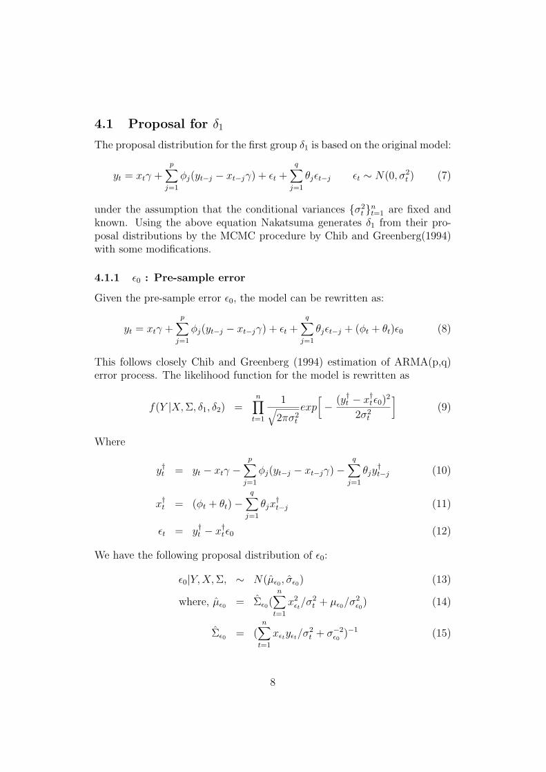
4.1.1 ε0 : Pre-sample error

Given the pre-sample error ε0, the model can be rewritten as:

yt = xtγ +p∑

j=1

φj(yt−j − xt−jγ) + εt +q∑

j=1

θjεt−j + (φt + θt)ε0 (8)

This follows closely Chib and Greenberg (1994) estimation of ARMA(p,q)error process. The likelihood function for the model is rewritten as

f(Y |X,Σ, δ1, δ2) =n∏

t=1

1√2πσ2

t

exp[− (y†t − x†tε0)

2

2σ2t

](9)

Where

y†t = yt − xtγ −p∑

j=1

φj(yt−j − xt−jγ)−q∑

j=1

θjy†t−j (10)

x†t = (φt + θt)−q∑

j=1

θjx†t−j (11)

εt = y†t − x†tε0 (12)

We have the following proposal distribution of ε0:

ε0|Y,X,Σ, ∼ N(µε0 , σε0) (13)

where, µε0 = Σε0(n∑

t=1

x2εt/σ2

t + µε0/σ2ε0

) (14)

Σε0 = (n∑

t=1

xεtyεt/σ2t + σ−2

ε0)−1 (15)

8

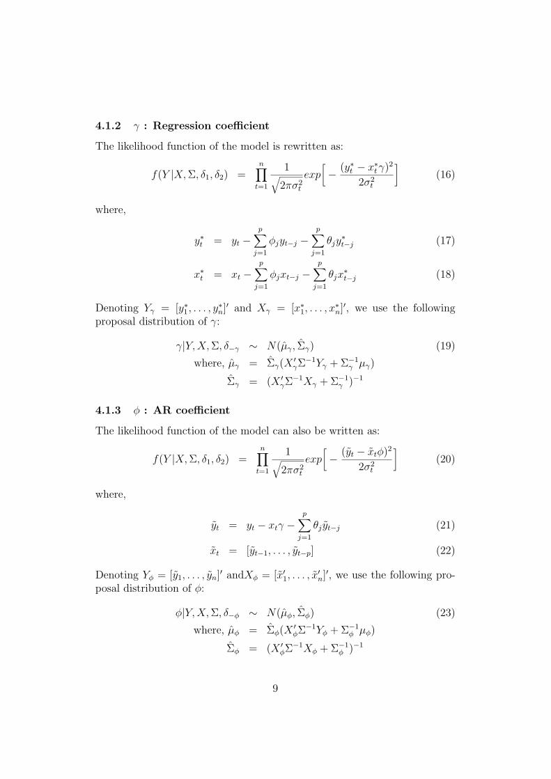
4.1.2 γ : Regression coefficient

The likelihood function of the model is rewritten as:

f(Y |X,Σ, δ1, δ2) =n∏

t=1

1√2πσ2

t

exp[− (y∗t − x∗tγ)

2

2σ2t

](16)

where,

y∗t = yt −p∑

j=1

φjyt−j −p∑

j=1

θjy∗t−j (17)

x∗t = xt −p∑

j=1

φjxt−j −p∑

j=1

θjx∗t−j (18)

Denoting Yγ = [y∗1, . . . , y∗n]′ and Xγ = [x∗1, . . . , x

∗n]′, we use the following

proposal distribution of γ:

γ|Y,X,Σ, δ−γ ∼ N(µγ, Σγ) (19)

where, µγ = Σγ(X′γΣ

−1Yγ + Σ−1γ µγ)

Σγ = (X ′γΣ

−1Xγ + Σ−1γ )−1

4.1.3 φ : AR coefficient

The likelihood function of the model can also be written as:

f(Y |X,Σ, δ1, δ2) =n∏

t=1

1√2πσ2

t

exp[− (yt − xtφ)2

2σ2t

](20)

where,

yt = yt − xtγ −p∑

j=1

θj yt−j (21)

xt = [yt−1, . . . , yt−p] (22)

Denoting Yφ = [y1, . . . , yn]′ andXφ = [x′1, . . . , x′n]′, we use the following pro-

posal distribution of φ:

φ|Y,X,Σ, δ−φ ∼ N(µφ, Σφ) (23)

where, µφ = Σφ(X′φΣ

−1Yφ + Σ−1φ µφ)

Σφ = (X ′φΣ

−1Xφ + Σ−1φ )−1

9

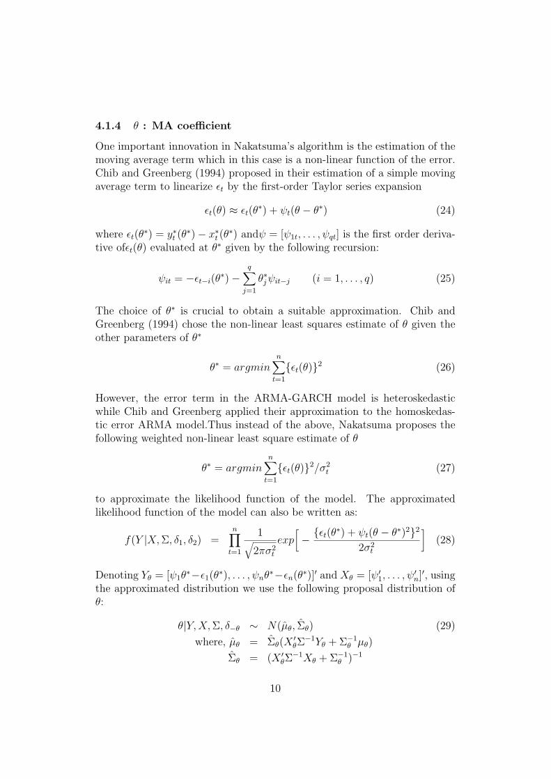
4.1.4 θ : MA coefficient

One important innovation in Nakatsuma’s algorithm is the estimation of themoving average term which in this case is a non-linear function of the error.Chib and Greenberg (1994) proposed in their estimation of a simple movingaverage term to linearize εt by the first-order Taylor series expansion

εt(θ) ≈ εt(θ∗) + ψt(θ − θ∗) (24)

where εt(θ∗) = y∗t (θ

∗)− x∗t (θ∗) andψ = [ψ1t, . . . , ψqt] is the first order deriva-

tive ofεt(θ) evaluated at θ∗ given by the following recursion:

ψit = −εt−i(θ∗)−

q∑j=1

θ∗jψit−j (i = 1, . . . , q) (25)

The choice of θ∗ is crucial to obtain a suitable approximation. Chib andGreenberg (1994) chose the non-linear least squares estimate of θ given theother parameters of θ∗

θ∗ = argminn∑

t=1

{εt(θ)}2 (26)

However, the error term in the ARMA-GARCH model is heteroskedasticwhile Chib and Greenberg applied their approximation to the homoskedas-tic error ARMA model.Thus instead of the above, Nakatsuma proposes thefollowing weighted non-linear least square estimate of θ

θ∗ = argminn∑

t=1

{εt(θ)}2/σ2t (27)

to approximate the likelihood function of the model. The approximatedlikelihood function of the model can also be written as:

f(Y |X,Σ, δ1, δ2) =n∏

t=1

1√2πσ2

t

exp[− {εt(θ∗) + ψt(θ − θ∗)2}2

2σ2t

](28)

Denoting Yθ = [ψ1θ∗−ε1(θ∗), . . . , ψnθ

∗−εn(θ∗)]′ and Xθ = [ψ′1, . . . , ψ

′n]′, using

the approximated distribution we use the following proposal distribution ofθ:

θ|Y,X,Σ, δ−θ ∼ N(µθ, Σθ) (29)

where, µθ = Σθ(X′θΣ

−1Yθ + Σ−1θ µθ)

Σθ = (X ′θΣ

−1Xθ + Σ−1θ )−1

10

4.2 Proposal for δ2

The proposal distribution for the second group δ2 are based on an approxi-mated GARCH model:

ε2t = µ0 + µ1St +l∑

j=1

(αj + βj)ε2t−j + wt −

s∑j=1

βjwt−j + αtw0 (30)

wt ∼ N(0, 2σ4t )

Given {ε2t}nt=1 and conditional variances {σ2

t }nt=1 it is possible to generate δ2

from their proposal distributions by the MCMC procedure similar to Chiband Greenberg’s method. However, before obtaining the ARCH and theGARCH coefficients, the next important step would be to obtain the statevariables in the variance expression.

The Markov Switching Process

At this point, we need to discuss the Bayesian estimation procedure for theMarkov Switching states. Let St be a stochastic variable taking the values0 or 1. Furthermore, we assume St evolves according to a Markov Chain,independent of past observations of yt i.e.,

P [St = j|St−1 = i, St−2 = i′, ....., yt−1] = P [St = j|St−1 = i] = pij (31)

The pij’s will be elements of a (2 × 2) transition matrix of states P whichcollects probability of going to state j at time t given being at state i at timet− 1.

P =

[p00 p10

p01 p11

](32)

The columns should sum to unity. So that we can write P as

P =

[q 1− p

1− q p

](33)

Assuming we have complete information about the vector of parameters{µ0, µ1} and the transition probabilities pij, we collect them into a setθ. If wehave a sequence of observation on yt for t ∈ {0, T} we now want to calculatethe likelihood of these observations as a function of the parameter vector θand the sequence of the state probabilities P [St = 0|yt; θ, P (St−1 = 1)] for

11

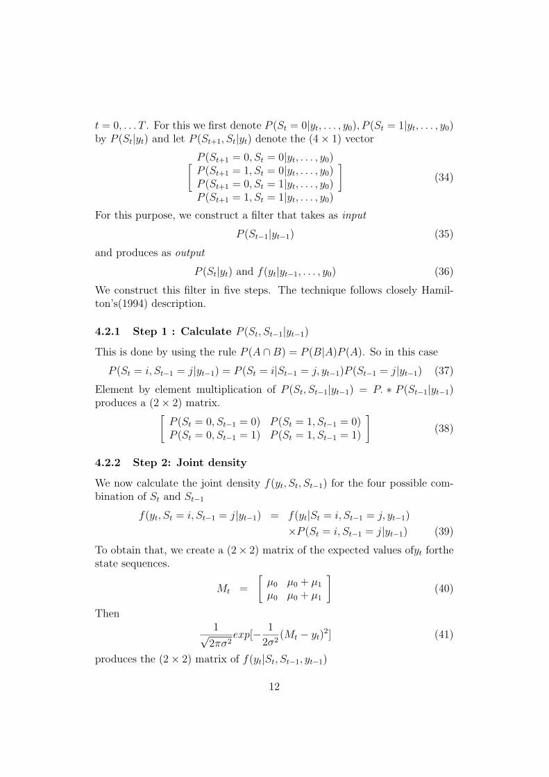
t = 0, . . . T . For this we first denote P (St = 0|yt, . . . , y0), P (St = 1|yt, . . . , y0)by P (St|yt) and let P (St+1, St|yt) denote the (4× 1) vector

[ P (St+1 = 0, St = 0|yt, . . . , y0)P (St+1 = 1, St = 0|yt, . . . , y0)P (St+1 = 0, St = 1|yt, . . . , y0)P (St+1 = 1, St = 1|yt, . . . , y0)

](34)

For this purpose, we construct a filter that takes as input

P (St−1|yt−1) (35)

and produces as output

P (St|yt) and f(yt|yt−1, . . . , y0) (36)

We construct this filter in five steps. The technique follows closely Hamil-ton’s(1994) description.

4.2.1 Step 1 : Calculate P (St, St−1|yt−1)

This is done by using the rule P (A ∩B) = P (B|A)P (A). So in this case

P (St = i, St−1 = j|yt−1) = P (St = i|St−1 = j, yt−1)P (St−1 = j|yt−1) (37)

Element by element multiplication of P (St, St−1|yt−1) = P. ∗ P (St−1|yt−1)produces a (2× 2) matrix.[

P (St = 0, St−1 = 0) P (St = 1, St−1 = 0)P (St = 0, St−1 = 1) P (St = 1, St−1 = 1)

](38)

4.2.2 Step 2: Joint density

We now calculate the joint density f(yt, St, St−1) for the four possible com-bination of St and St−1

f(yt, St = i, St−1 = j|yt−1) = f(yt|St = i, St−1 = j, yt−1)

×P (St = i, St−1 = j|yt−1) (39)

To obtain that, we create a (2× 2) matrix of the expected values ofyt forthestate sequences.

Mt =

[µ0 µ0 + µ1

µ0 µ0 + µ1

](40)

Then1√

2πσ2exp[− 1

2σ2(Mt − yt)

2] (41)

produces the (2× 2) matrix of f(yt|St, St−1, yt−1)

12

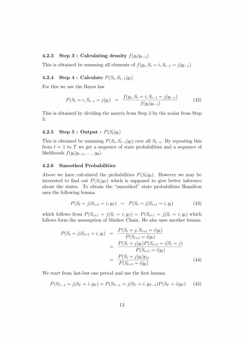
4.2.3 Step 3 : Calculating density f(yt|yt−1)

This is obtained be summing all elements of f(yt, St = i, St−1 = j|yt−1)

4.2.4 Step 4 : Calculate P (St, St−1|yt)

For this we use the Bayes law

P (St = i, St−1 = j|yt) =f(yt, St = i, St−1 = j|yt−1)

f(yt|yt−1)(42)

This is obtained by dividing the matrix from Step 2 by the scalar from Step3.

4.2.5 Step 5 : Output : P (St|yt)

This is obtained be summing P (St, St−1|yt) over all St−1. By repeating thisfrom t = 1 to T we get a sequence of state probabilities and a sequence oflikelihoods f(yt|yt−1, . . . , y0).

4.2.6 Smoothed Probabilities

Above we have calculated the probabilities P (St|yt). However we may beinterested to find out P (St|yT ) which is supposed to give better inferenceabout the states. To obtain the “smoothed” state probabilities Hamiltonuses the following lemma

P (St = j|St+1 = i, yT ) = P (St = j|St+1 = i, yt) (43)

which follows from P (St+1 = j|St = i, yT ) = P (St+1 = j|St = i, yt) whichfollows form the assumption of Markov Chain. He also uses another lemma

P (St = j|St+1 = i, yt) =P (St = j, St+1 = i|yt)

P (St+1 = i|yt)

=P (St = j|yt)P (St+1 = i|St = j)

P (St+1 = i|yt)

=P (St = j|yt)pji

P (St+1 = i|yt)(44)

We start from last-but-one period and use the first lemma:

P (ST−1 = j|ST = i, yT ) = P (ST−1 = j|ST = i, yT−1)P (ST = i|yT ) (45)

13

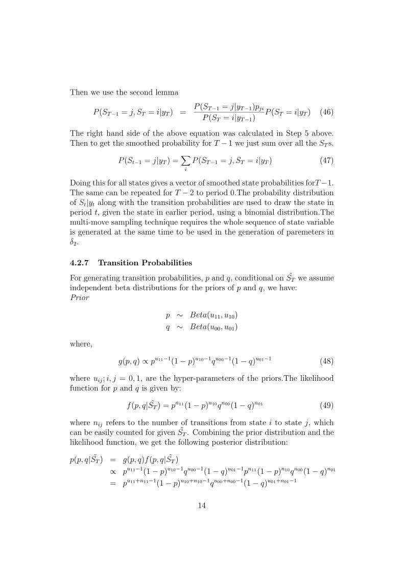
Then we use the second lemma

P (ST−1 = j, ST = i|yT ) =P (ST−1 = j|yT−1)pji

P (ST = i|yT−1)P (ST = i|yT ) (46)

The right hand side of the above equation was calculated in Step 5 above.Then to get the smoothed probability for T − 1 we just sum over all the ST s.

P (St−1 = j|yT ) =∑

i

P (ST−1 = j, ST = i|yT ) (47)

Doing this for all states gives a vector of smoothed state probabilities forT−1.The same can be repeated for T − 2 to period 0.The probability distributionof St|yt along with the transition probabilities are used to draw the state inperiod t, given the state in earlier period, using a binomial distribution.Themulti-move sampling technique requires the whole sequence of state variableis generated at the same time to be used in the generation of paremeters inδ2.

4.2.7 Transition Probabilities

For generating transition probabilities, p and q, conditional on ST we assumeindependent beta distributions for the priors of p and q, we have:Prior

p ∼ Beta(u11, u10)

q ∼ Beta(u00, u01)

where,

g(p, q) ∝ pu11−1(1− p)u10−1qu00−1(1− q)u01−1 (48)

where uij; i, j = 0, 1, are the hyper-parameters of the priors.The likelihoodfunction for p and q is given by:

f(p, q|ST ) = pn11(1− p)n10qn00(1− q)n01 (49)

where nij refers to the number of transitions from state i to state j, whichcan be easily counted for given ST . Combining the prior distribution and thelikelihood function, we get the following posterior distribution:

p(p, q|ST ) = g(p, q)f(p, q|ST )

∝ pu11−1(1− p)u10−1qu00−1(1− q)u01−1pn11(1− p)n10qn00(1− q)n01

= pu11+n11−1(1− p)u10+n10−1qu00+n00−1(1− q)u01+n01−1

14

4.3 α : ARCH coefficient

The likelihood function of the approximated GARCH model is rewritten as

f(ε2t |Y,X,Σ, δ1, δ2) =n∏

t=1

1√2π(2σ4

t )exp

[− (ε2t − ζtα)2

2(2σ4t )

](50)

where ε2 = [ε21, . . . , ε2n]′ , ε2t = ε2t −

∑sj=1 βj ε

2t−j andζt = [ιt, ε

2t−1, . . . , εt−r].

Let Yα = [ε21, . . . , ε2n]′ andXα = [ζ ′1, . . . , ζ

′n]′. We have the following proposald-

istribution of α:

α|Y,X,Σ, δ−α ∼ N(µα, Σα) (51)

where, µα = Σα(X ′αΛ−1Yα + Σ−1

α µα)

Σα = (X ′αΛ−1Xα + Σ−1

α )−1

Λ = diag{2σ41, . . . , 2σ

4n}

4.4 β : GARCH coefficient

The likelihood function of the approximated GARCH model is rewritten as

f(ε2|Y,X,Σ, δ1, δ2) =n∏

t=1

1√2π(2σ4

t )exp

[− {wt(β

∗)− ξt(β − β∗)}2

2(2σ4t )

](52)

where ξt = [ξ1t, ξ2t] is the first-order derivative of σ2t (β) evaluated at β∗.

Let Yβ = [w1(β∗)+ξ1β

∗, . . . , wn(β∗)+ξnβ∗]′and Xβ = [ξ′1, . . . , ξ

′n]′. Using the

approximated likelihood function, we have the following proposal distributionof β:

β|Y,X,Σ, δβ ∼ N(µβ, Σβ) (53)

where, µβ = Σβ(X ′βΛ−1Yβ + Σ−1

β µβ)

Σβ = (X ′βΛ−1Xβ + Σ−1

β )−1

Λ = diag{2σ41, . . . , 2σ

4n}

5 Results and Conclusions

We apply the algorithms for a ARMA(1,1) Markov Switching GARCH modelon simulated data and also on a market data set. The market data that isbeing considered is one of the most important market index in Indian Stockmarket, the Bombay Stock Exchange (BSE) SENSEX, which is composed ofa basket of 30 Indian stocks. The above procedure was implemented on asimulated Switching GARCH data and the results are as follows:

15

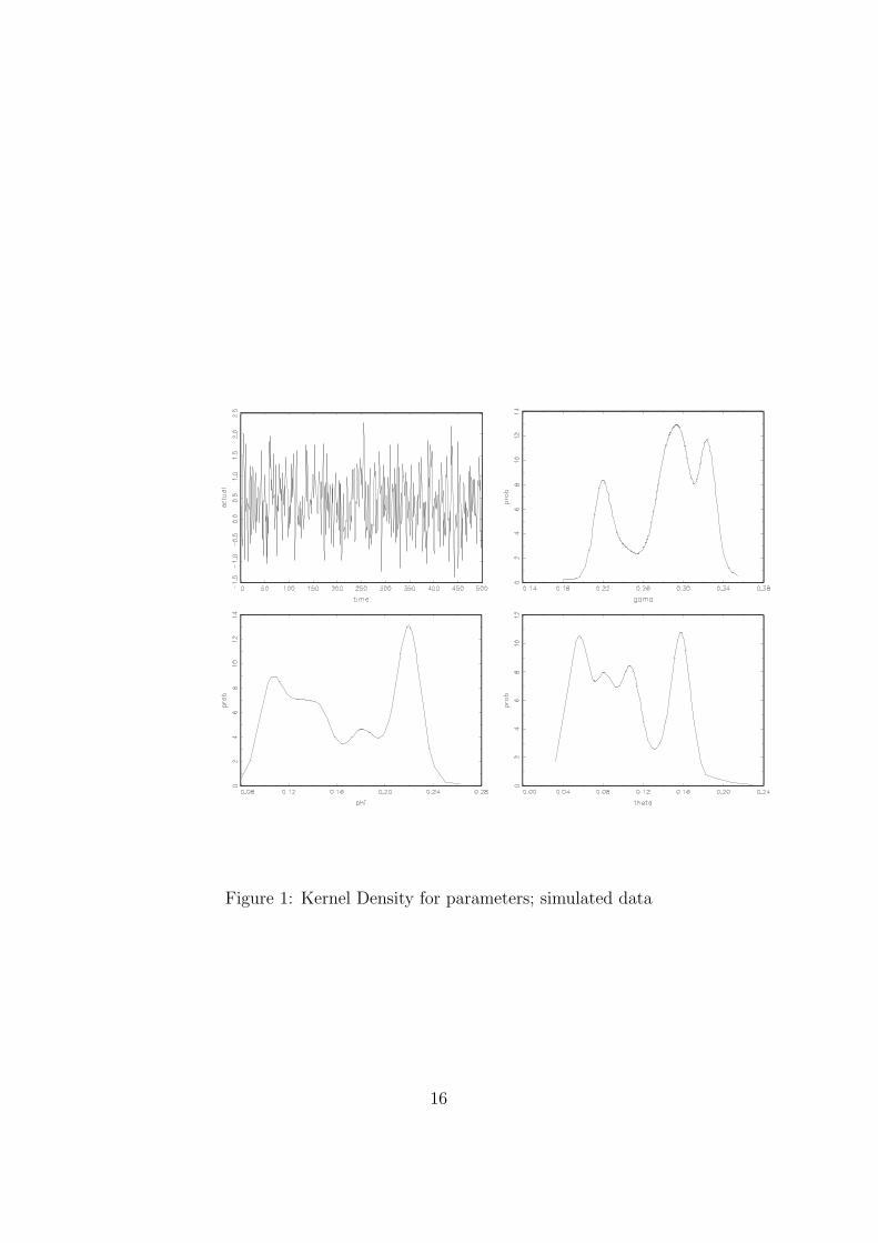
Figure 1: Kernel Density for parameters; simulated data

16

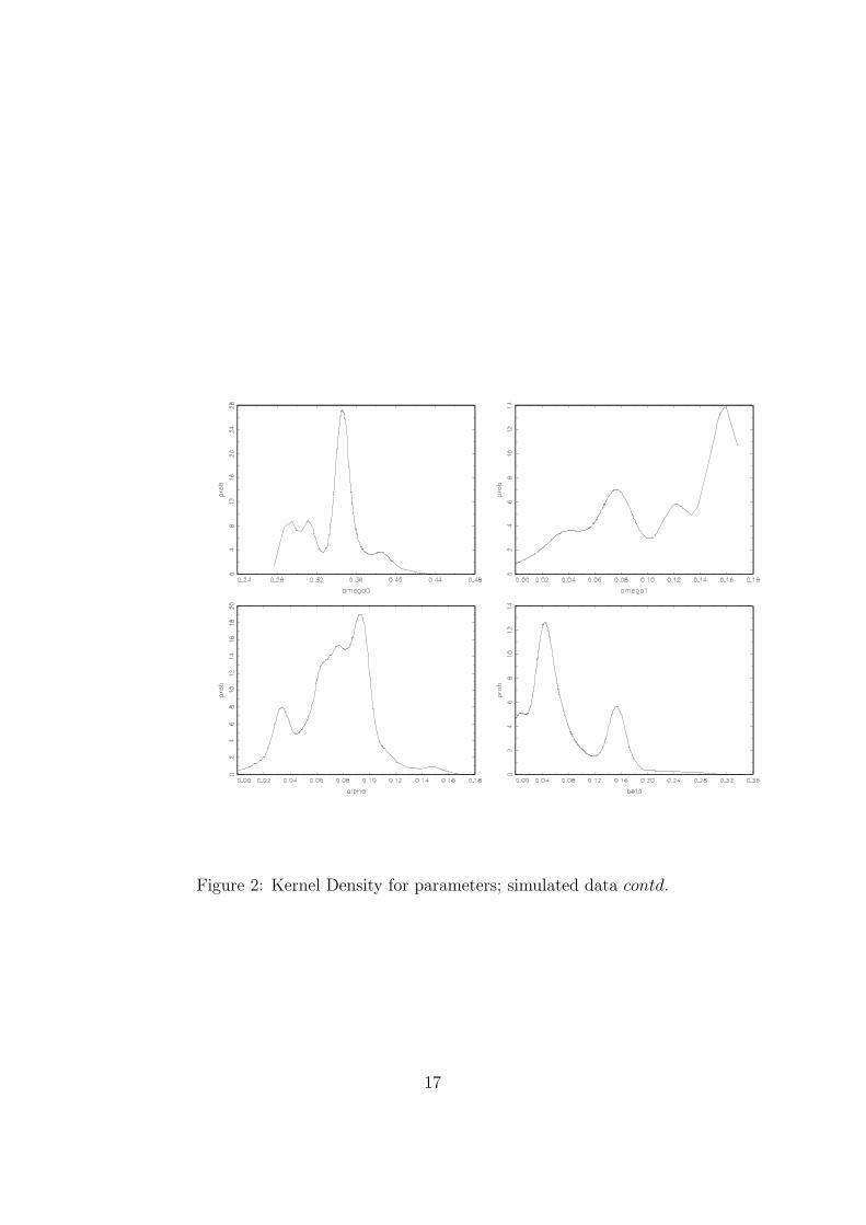
Figure 2: Kernel Density for parameters; simulated data contd.

17

Parameters Original values Estimated values Standard deviation

γ 0.3000 0.2820 0.0383φ 0.1000 0.1657 0.0462θ 0.1000 0.1032 0.0419ω0 0.3000 0.3360 0.0289ω1 0.1000 0.1141 0.0481α 0.1000 0.0742 0.0267β 0.1000 0.0725 0.0567

The model seems to have satisfactory performance with respect to the originalvalues.The same algorithm is then applied on the BSE sensex data and theresults are asfollows:

Parameters Estimated values Standard deviation

γ -0.1081 0.0696φ 0.5337 0.0439θ -0.4286 0.0563ω0 1.0398 0.1841ω1 0.5640 0.1793α 0.1516 0.0210β 0.6118 0.0750

The statistical significance of the switching parameter makes the point re-garding the applicability of a Markov switching GARCH model on the marketdata.

Conclusion

Time series processes study systems, whose dynamics are strongly depen-dent on itself or past values of related variables. Considerable informationcan however be also gained from the second moments. The GARCH modeladvanced the understanding of time series process by incorporating the sec-ond moments. A Markov Switching GARCH process accomodates furtherthe aspect of time series dynamics being affected by external unpredictableprocesses. Incorporating a Markov Switching process for the conditionalvariance of the underlying asset prices will only enhance predictive power.Literature on derivative pricing generally does not consider these aspects ofthe time dynamics, which are so common in observed data. Previously the

18

Figure 3: Kernel Density for parameters; BSE Sensex data

19

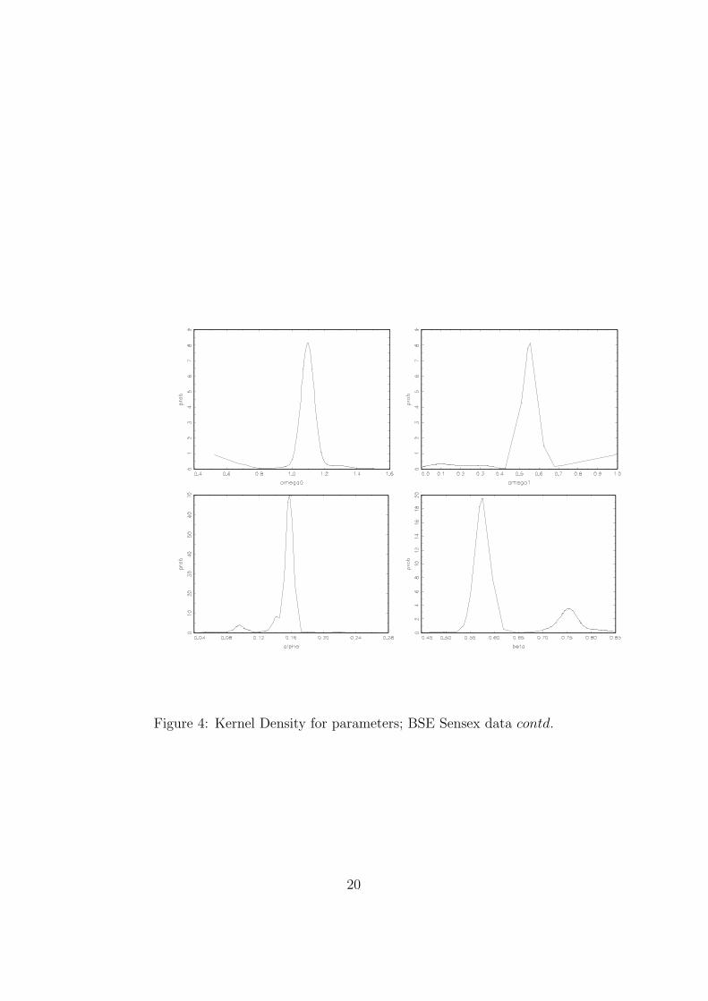
Figure 4: Kernel Density for parameters; BSE Sensex data contd.

20

variances were plugged into the Black Scholes option pricing formula (En-gle, Hong, Kane and Noh(1993)). Recently Duan (89) developed a GARCHoption-pricing model, where he introduced the concept of local risk neutralvaluation with respect to an underlying GARCH asset pricing process. Us-ing local risk neutral valuation, the Markov Switching GARCH can also beapplied in derivative pricing. Further research in this area requires the clari-fication of certain aspects of the Bayesian estimation technique. We need tolook into the convergence of the MCMC draws using plots and test statis-tic such as the fluctuation test discussed in Goldman, Valieva and Tsurumi(2003). We should also look at identification and the applicability of the filterthat generates the state probabilities for a more precise algorithm for estimat-ing such processes as discussed in Kaufman and Fruhwirth-Schnatter (2002).In addition, the performance of this technique in comparison to other spec-ifications of asymmetric GARCH model should be investigated using Bayesfactor and predictive densities.

References

[1] J. Albert and S. Chib. A Markov model of unconditional variance inARCH. Journal of Econometrics, 58, 1993.

[2] R.T. Baillie and T. Bollerslev. Prediction in Dynamic Models withTime-Dependent Conditional Variances. Journal of Econometrics, 52,1992.

[3] R. Barnett, G. Kohn and S. Sheather. Bayesian estimation of an au-toregressive model using Markov Chain Monte Carlo. Journal of Econo-metrics, 74, 1996.

[4] L. Bauwens and M. Lubrano. Bayesian inference on GARCH modelsusing Gibbs sampler. Econometrics Journal, 1, 1998.

[5] A.K. Bera and H.L. Higgins. A Survey of ARCH Models: Properties,Estimation and Testing. Journal of Economic Surveys, 4, 1993.

[6] O.J. Blanchard and M.W. Watson. Bubbles, rational expectations andfinancial markets. Lexington Books, 1982.

[7] S. F. Bollen, N. P. B. Gray and Whaley R. E. Regime switching inforeign exchange rates: Evidence from currency option prices. Journalof Econometrics, 94, 2000.

21

[8] T. Bollerslev. Generalized autoregressive conditional heteroskedasticity.Journal of Econometrics, 31, 1986.

[9] G. Box and G. Jenkins. Time Series Analysis: Forecasting and Control.Holden-Day, 1976.

[10] J. Cai. Bayes Regression and Autocorrelated Errors: A Gibbs SampleApproach. Journal of Business and Economic Statistics, 12, 1994.

[11] B. P. Carlin and A.E. Gelfand. Approaches for Empirical Bayes Con-fidence Intervals. Journal of the American Statistical Association, 85,1990.

[12] N. G. Carlin, B.P. Polson and D.S. Stoffer. A Monte Carlo Approach toNonnormal and Nonlinear State-Space Modeling. Journal of the Amer-ican Statistical Association, 87, 1992.

[13] C. Carter and R. Kohn. On Gibbs Sampling for State Space Models.Biometrika, (81), 1994.

[14] P. Cecchetti, S. G. Lam and M. Nelson. Mean Reversion in EquilibriumAsset Prices. American Economic Review, 80, 1990.

[15] S. Chib and E. Greenberg. Understanding the Metropolis Hastings Al-gorithm. The American Statistician, 49, 1995.

[16] F. X. Diebold. Modeling the Persistence of Conditional Variances: AComment. Econometric Reviews, 5, 1986.

[17] J. C. Duan. The GARCH option Pricing model. Mathematical Finance,1995.

[18] M. Dueker. Markov Switching in GARCH Processes and Mean- Revert-ing Stock Market Volatility. Journal of Business and Economic Statis-tics, 15, 1997.

[19] R. Engle and C. Mustafa. Implied ARCH Models from Option Prices.Journal of Econometrics, 52, 1992.

[20] R. F. Engle. Autoregressive conditional heteroskedasticity with esti-mates of the variance of United Kingdom inflation. Econometrica, 50,1982.

[21] E. F. Fama. The Behaviour of Stock Market Prices. Journal of Business,38, 1965.

22

[22] J. Geweke. Bayesian Inference in Econometric Models Using MonteCarlo Integration. Econometrica, 57, 1989.

[23] R. Glosten, L.R. Jagannathan and D.E. Runkle. On the Relation be-tween Expected Value and the Volatility of the Nominal Excess Returnon Stocks. The Journal of Finance, 48, 1993.

[24] S. Goldfeld and R. Quandt. A Markov Model for Switching Regression.Journal of Econometrics, 1, 1973.

[25] E. Goldman, E. Valieva and H. Tsurumi. Convergence Tests for MarkovChain Monte Carlo Draws. Technical report, Rutgers University, 2003.

[26] J Hamilton. A New Approach to the Economic Analysis of Nonstation-ary Time Series and the Business Cycle. Econometrica, 57, 1989.

[27] J. Hamilton. Time Series Analysis. Princeton University Press, 1994.

[28] J. Hamilton and R. Susmel. Autoregressive Conditional Heteroskedas-ticity and Changes in Regime. Journal of Econometrics, 64, 1994.

[29] B. E. Hansen. Autoregressive Conditional Density Estimation. Interna-tional Economic Review, 35, 1994.

[30] W. K. Hastings. Monte Carlo sampling methods using Markov chainsand their applications. Biometrika, (57), 1970.

[31] S. L. Heston and S. Nandi. A Closed-Form GARCH Option PricingModel. Working Papers, 1997. Federal Reserve Bank of Atlanta.

[32] S. Kaufmann and S. Fruhwirth-Schnatter. Bayesian Analysis of Switch-ing ARCH Models. Journal of Time Series Analysis, 23, 2002.

[33] C. Kim and C. Nelson. State Space Models with Regime Switching:Classical and Gibbs Sampling Approaches with Aplications. MIT Press,Cambridge, 1999.

[34] F. Kleibergen and H.K. van Dijk. Nonstationarity in GARCH Models:A Bayesian Analysis. Journal of Applied Econometrics, 8, 1993.

[35] C. Lamoreux and W. Lastrapes. Persistence in Variance, StructuralChange and the GARCH Model. Journal of Business and EconomicStatistics, 5, 1990.

[36] B.B. Mandelbrot. New methods in statistical economics. Journal ofPolitical Economy, 71, 1963.

23

[37] M.N. Metropolis N.; Rosenbluth, A.W.; Rosenbluth and Teller A.H.Equation of State Calculations by Fast Computer Machines. Journal ofChemical Physics, 21, 1953.

[38] P. Muller and A. Pole. Monte Carlo Posterior Integration in GARCHmodels. Sankhya, 6, 1998.

[39] T. Nakatsuma. A Markov-Chain Sampling Algorithm for GARCH Mod-els. Studies in Nonlinear Dynamics and Econometrics, 3, 1998.

[40] T. Nakatsuma. Bayesian analyisis of ARMA-GARCH models: A Markovchain sampling approach. Journal of Econometrics, 95, 2000.

[41] D. B. Nelson. Conditional heteroskedasticity in asset pricing: a newapproach. Econometrica, 59, 1991.

[42] R. Rabemananjara and J. M. Zakoian. Threshold ARCH Models andAsymmetries in Volatility. Journal of Applied Econometrics, 1, 1993.

[43] C. Ritter and M. Tanner. Facilitating the Gibbs Sampler: The GibbsStopper and the Griddy-Gibbs Sampler. Journal of American StatisticalAssociation, 87(419), 1992.

[44] C. P. Robert and G. Casella. Monte Carlo Statistical Methods. Springer,1999.

[45] G. W. Schwert. Why Does Stock Market Volatility Change Over Time?Journal of Finance, 44, 1989.

[46] G. W. Schwert. Stock volatility and the crash of ’87. Review of FinanicalStudies, 3, 1990.

[47] E. Sentana. Quadratic ARCH Models. Review of Economic Studies, 62,1995.

[48] R. Susmel. Switching Volatility in International Equity Markets. Journalof Econometrics, 1992.

[49] H. Tsurumi. Bayesian Statistical Computations of Nonlinear FinancialTime Series Models: A Survey with Illustrations. Asia-Pacific FinancialMarkets, 7, 2000.

[50] R. Turner, C. Startz and C. Nelson. A Markov model of heteroscedas-ticity, risk, and learning in the stock market. Journal of Financial Eco-nomics, 25, 1989.

24

[51] S. vanNorden and H. Schaller. Regime Switching in Stock Market Re-turns. Technical report, Bank of Canada, 1993. Working Papers.

[52] G. Wei and M. Tanner. A Monte Carlo implementation of the EMalgorithm and the poor mans data augmentation algorithms. Journal ofthe American Statistical Association, 85, 1990.

25