A Approach to Commercial Real Estate...

0

A Comprehensive Approach to Commercial Real Estate Prices1

By

Ruijue Peng PPR, A CoStar Company

33 Arch Street Boston, MA 02110 (617) 443 3198

[email protected]

Andrew C. Florance CoStar

1331 L Street, NW Washington, DC 20005‐4101

(202) 346‐6500 [email protected]

Mingjun Huang Barclays Capital (574) 229‐4886

[email protected]

Norm Miller University of San Diego

(619) 260‐7939 [email protected]

Karl E. Case

Wellesley College (781) 283‐2178

[email protected]

1 This paper was presented at the 2010 ARES conference and won the award for “The Best Paper by A Practitioner.”

1

A Comprehensive Approach to Commercial Real Estate Prices

ABSTRACT

The CRE market is characterized by heterogeneity and a high degree of segmentation, creating a

challenge for developing a comprehensive CRE price index. Existing indices in the market place have

primarily focused on high‐value transactions — a small fraction of total CRE transactions. To capture the

multifaceted and diverse picture of the CRE market, we explored alternative repeat‐sale indexing

methodologies to determine the most appropriate approach. We found that conventional methods

using prices as breakpoints for determining market tiers produced biased indices. Our indices were thus

developed based on datasets defined by physical characteristics of properties. We concluded that using

a consistent indexing methodology to track mutually exclusive market segments is the most accurate,

straightforward, and comprehensive approach.

I. BACKGROUND

The CoStar Commercial Repeat‐Sale Index (CCRSI) was developed by using the repeat‐sale regression

technique, which has been increasingly accepted as the most clear‐cut and sufficiently rigorous method

to meet investors’ requirements. The repeat‐sale analysis, based on properties that have sold more than

once without any significant change in building characteristics between sales, is fundamentally

comparable to stock and bond indices, which are based on stock (or bond) price changes from one

period to the next. In real estate, the most well‐known repeat‐sale index is the Standard & Poor's Case–

Shiller Home Price Index. Not only has the Case‐Shiller Index become the barometer of the health of the

nation’s housing market, it has also been used by the Chicago Mercantile Exchange to support and

facilitate derivatives trading against housing. OFHEO’s Home Price Index is another example of a repeat‐

sale‐based index that has been widely used and cited in the residential housing market.

In the CRE market place, the most commonly used price index to date is the one produced by the

National Council of Real Estate Investments Fiduciaries (NCREIF). The NCREIF Index is appraisal‐based

rather than transaction‐based and is derived from a small data sample that consists solely of large and

prime properties owned by pension fund investors. The Moody’s/Real CPPI was the first CRE repeat‐sale

index, developed in 2007. However, the use of this index is limited by the lack of comprehensive data

coverage. CPPI is based on transaction data from Real Capital Analytics (RCA), which has approximately

10 years of history and focuses only on high‐value transactions. RCA data initially covered transactions

of $5 million‐up and extended to $2.5 million‐up in 2005.

CoStar began collecting CRE transaction data 20 years ago and has a total of 1.33 million CRE property

sales records in its database. It covers CRE transactions across the United States in all price ranges. This

extensive database with a long history contains a large number of repeat transactions from which we

were able to develop consistent and comprehensive price indices.

2

II. DATA & FEATURE EXTRACTION

Accurate identification of repeat‐sale pairs is critical to building an accurate index that reflects market

conditions excluding all other non‐market factors. We therefore applied three stages of filtering to the

CoStar transaction database to obtain the final sales pairs. In the first stage, we extracted a dataset

containing properties that were sold more than once. We compared multiple building characteristics to

ensure that two transactions were indeed the same asset. In the second stage, we set up 32

exclusionary criteria to filter out non‐representative transactions, such as portfolio sales, non‐arm’s‐

length transactions, and build‐to‐suit transactions. Also excluded were properties below a minimum

physical threshold of square footage and units.

The third stage of data filtering mainly targeted “flippers” — those properties sold more than once

within a short period of time — and “outliers,” properties with abnormal price increases. Both were

identified empirically. As Chart 1 shows, most transactions occurred after a 12‐month holding period,

which is consistent with generally accepted practice because of U.S. tax considerations. Therefore,

transactions occurring in less than a 12‐month period are filtered out as “flippers.”

CHART 1

0

200

400

600

800

1,000

1,200

1,400

1,600

1,800

2,000

0 12 24 36 48 60 72 84 96 108 120 132 144 156 168 180

Months between two sales

Pair Counts by Holding Period

Chart 2 shows pair distribution by the average annual price change. Most of the pairs cluster around the

10% to 20% range. The pair counts decrease quickly in both directions. Roughly 98% of the total pairs

fall into the range between ‐40% and 50%. We thus excluded the pairs at the extreme ends of the

spectrum as “outliers” for all property types except for land. The range for land is ‐50% to 60% because

it has a much wider and flatter distribution.

3

CHART 2

0

5,000

10,000

15,000

20,000

25,000

30,000

35,000

[-0.

4, -

0.3)

[-0.

3, -

0.2)

[-0.

2, -

0.1)

[-0.

1, 0

)

[0, 0

.1)

[0.1

, 0.2

)

[0.2

, 0.3

)

[0.3

, 0.4

)

[0.4

, 0.5

]

Pair Distribution by Average Annual Price Change

After the filtering process, our final dataset had a total of 85,428 repeat‐sale observations covering the

period 1996–2010. Chart 3 shows the distribution of repeat‐sale pair counts by property type and the

corresponding share of transaction value of each property type. Apartment ranks highest in the number

of repeat‐sale transactions, while office leads in the total value of transactions. This result is expected.

Office transactions occur less frequently than apartment sales, but offices tend to sell at higher prices.

CHART 3

APT, 35%

IND, 16%OFF, 17%

RET, 21%

Land, 4%

Flex, 3%

Hotel, 3%Other, 1%

Pair Counts

APT, 27%

IND, 9%

OFF, 41%

RET, 13%

Land, 2%

Flex, 3%Hotel, 5%

Other, 1%

Transaction Value

4

The relationship between transaction frequency and transaction value can be further illustrated by the

distribution of repeat‐sale pair counts over price brackets and the dollar value of transactions in each

bracket. As shown in Chart 4, most of the transaction activities are concentrated in the low price

bracket below $1.25 million. As prices increase, the number of transactions diminishes rapidly.

Transaction value, on the other hand, is concentrated in the high price brackets. In particular, those

transactions greater than $5 million account for the major share of total transaction value, even though

the number of these high‐priced transactions represents a small fraction of the total number of

transactions.

CHART 4

0

5000

10000

15000

20000

25000

30000

Pair Counts by Bucket ‐‐ All Types

$0

$20

$40

$60

$80

$100

$120

$140Billions

Transaction Value by Bucket ‐‐ All Types

Chart 5 shows the distribution patterns for each of the four major property types. The divergence of

transaction frequency and transaction value is significant for apartment. But it is most pronounced for

office properties, where the largest number of transactions occur in the brackets below $10 million, but

transactions priced above $10 million constitute most of the total transaction value. Industrial

properties, on the other hand, generally sell within a narrow price range, and as a result, we see

transaction activities and value both below $10 million. We would expect retail to show a divergence

similar to that of office. However high‐end retail transactions are underrepresented in our repeat‐sale

dataset due to the fact that retail transactions are generally included in multi‐asset portfolio sales. Also

the physical characteristics of retail properties change significantly from one sale to the next, which

makes retail transactions less likely to meet our criteria for repeat‐sale pairs.

5

CHART 5

0

2000

4000

6000

8000

10000

12000

Pair Counts by Bucket ‐‐ Apartment

$0

$10

$20

$30

$40

$50

Billions

Transaction Value by Bucket ‐‐ Apartment

0500

10001500200025003000350040004500

Pair Counts by Bucket ‐‐ Office

$0$5

$10$15$20$25$30$35$40$45

Billions

Transaction Value by Bucket ‐‐ Office

0

1000

2000

3000

4000

5000

6000

7000

Pair Counts by Bucket ‐‐ Retail

$0$2$4$6$8

$10$12$14$16$18

Billions

Transaction Value by Bucket ‐‐ Retail

0

1000

2000

3000

4000

5000

Pair Counts by Bucket ‐‐ Industrial

$0

$2

$4

$6

$8

$10

$12

Billions

Transaction Value by Bucket ‐‐ Industrial

6

Clearly, the heterogeneity of the CRE market is multi‐dimensional. There is general divergence between

transaction activities and values, and the degree of divergence varies across property types. It is this

complexity that differentiates CRE from the housing market and attracts different investors with

different investment goals, resulting in widely varying performances. Therefore, our goal is to capture

the diversity of CRE market and its unique behavior.

III. METHODOLOGY

Since the repeat‐sale regression was first introduced by Bailey, Muth, and Nourse (1963), significant

advances have been made by Case‐Shiller (1987), Case‐Shiller (1989), Shiller (1991), Goetzmann (1992),

Clapp‐Giacotto (1992), Gatzlaff‐Haurin (1997), and others. To date, there are two types of repeat‐sale

regression methodologies. The first most commonly used method treats every transaction equally,

regardless of the value of the transaction. The resulting index is an equal‐weighted, geometric mean

index. The second method, known as the arithmetic mean repeat‐sale regression, introduced by Shiller

in 1991, weighs price change by the value of each transaction. The Standard & Poor's Case–Shiller Home

Price Index, for example, is an arithmetic mean index. We explored both approaches in developing the

CoStar index. See Appendix 1 for a mathematic presentation of the two methodologies.

Generally speaking, the geometric, equal‐weighted methodology is more relevant for measuring the

performance of individual properties, while the arithmetic, value‐weighted index is a better measure of

overall market performance. For capturing CRE price movement, however, each method has its pros and

cons. Due to the difference between transaction frequency and transaction value, a single, equal‐

weighted index is inadequate. Because every transaction has the same impact on the results regardless

of transaction price, an equal‐weighted index will be biased towards low‐value deals where transaction

frequency is the highest.

The value‐weighted index, on the other hand, captures the heavy influence of the high‐end properties

on overall market value and can be particularly useful for asset allocation analysis. However, the value‐

weighted index is less relevant for broad investment activities because the majority of transactions

occur in the low‐value ranges. Also, the value‐weighted index may produce statistical noise since a few

very expensive sales will have a disproportionate impact on the results. Therefore, in practice, value‐

weighted methodology has limited applicability, unless there are sufficient data to mitigate the noise.

Table 1 illustrates the differences in the two approaches. All three scenarios under Up Market on the

left‐hand side have the same appreciation, but the sales prices are different. The equal‐weighted results

show the same overall price change for all three scenarios, while the value‐weighted results are tied

closely to the appreciation of higher prices. The same holds true in the Down Market scenarios. The

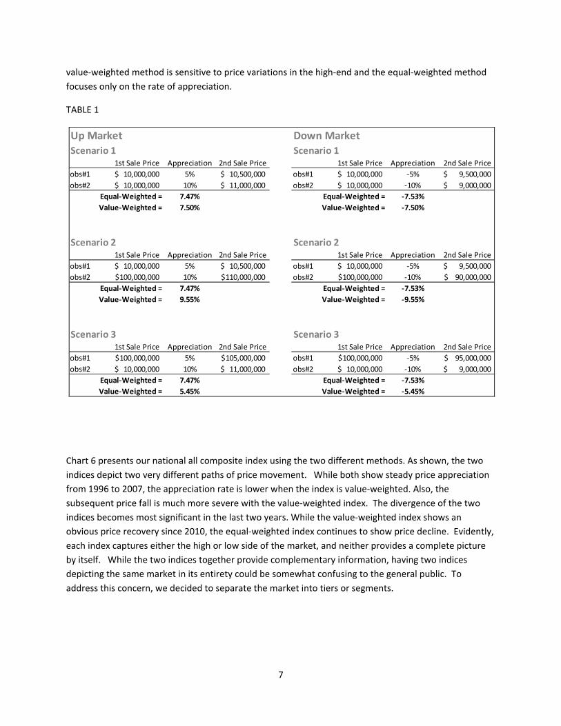
7

value‐weighted method is sensitive to price variations in the high‐end and the equal‐weighted method

focuses only on the rate of appreciation.

TABLE 1

Up Market Down MarketScenario 1 Scenario 1

1st Sale Price Appreciation 2nd Sale Price 1st Sale Price Appreciation 2nd Sale Price

obs#1 10,000,000$ 5% 10,500,000$ obs#1 10,000,000$ ‐5% 9,500,000$

obs#2 10,000,000$ 10% 11,000,000$ obs#2 10,000,000$ ‐10% 9,000,000$

Equal‐Weighted = 7.47% Equal‐Weighted = ‐7.53%

Value‐Weighted = 7.50% Value‐Weighted = ‐7.50%

Scenario 2 Scenario 21st Sale Price Appreciation 2nd Sale Price 1st Sale Price Appreciation 2nd Sale Price

obs#1 10,000,000$ 5% 10,500,000$ obs#1 10,000,000$ ‐5% 9,500,000$

obs#2 100,000,000$ 10% 110,000,000$ obs#2 100,000,000$ ‐10% 90,000,000$



Scenario 3 Scenario 31st Sale Price Appreciation 2nd Sale Price 1st Sale Price Appreciation 2nd Sale Price

obs#1 100,000,000$ 5% 105,000,000$ obs#1 100,000,000$ ‐5% 95,000,000$

obs#2 10,000,000$ 10% 11,000,000$ obs#2 10,000,000$ ‐10% 9,000,000$



Chart 6 presents our national all composite index using the two different methods. As shown, the two

indices depict two very different paths of price movement. While both show steady price appreciation

from 1996 to 2007, the appreciation rate is lower when the index is value‐weighted. Also, the

subsequent price fall is much more severe with the value‐weighted index. The divergence of the two

indices becomes most significant in the last two years. While the value‐weighted index shows an

obvious price recovery since 2010, the equal‐weighted index continues to show price decline. Evidently,

each index captures either the high or low side of the market, and neither provides a complete picture

by itself. While the two indices together provide complementary information, having two indices

depicting the same market in its entirety could be somewhat confusing to the general public. To

address this concern, we decided to separate the market into tiers or segments.

8

CHART 6

0

50

100

150

200

250

Mar-96

Mar-97

Mar-98

Mar-99

Mar-00

Mar-01

Mar-02

Mar-03

Mar-04

Mar-05

Mar-06

Mar-07

Mar-08

Mar-09

Mar-10

Value-Weighted All Equal-Weighted All

However, our efforts to divide transactions into market tiers illuminated some issues in the current

practice of segmenting properties by price breakpoints. In the CRE marketplace, $5 million and $2.5

million are the traditional cut‐off points for determining what is high‐end and what is low‐end. In the

course of our research, we discovered that segmenting market transactions by price breakpoints has

great potential to bias the resulting index.

Table 2 presents the results of our simulations demonstrating how price based cut‐offs produce bias for

the high‐end tier. There are four possible ways to divide a market using transaction prices. If the first

sale price is the cut‐off point, the resulting index will capture falling prices, but not rising prices, resulting

in downward bias. Conversely, using the second‐sale price as the breakpoint, results in an upward bias.

If both first and second sale prices are required to be greater than a certain price breakpoint, then price

movements are pushed below the breakpoint into a lower priced market segment, resulting in an

understatement of volatility. Using either the first sale or the second sale price as breakpoints, on the

other hand, draws in price movements from the market segment below the breakpoints, resulting in an

overstatement of volatility.

In summary, the simulation results of four possible cuts show that using the first sale price generates the

lowest average annual growth, 2.9%, whereas using the second sales price results in the highest annual

growth rate, 7.7%. While the either / or approach generates the highest volatility, 12.2%, using both

sales prices results in the lowest volatility, 9.6%.

9

TABLE 2

First Sale Price > 2.5 Million Second Sale Price > 2.5 Million

Downward Bias Upward Bias

Peak to Trough: 45% Peak to Trough: 31%

Average Annual Growth: 2.9% Average Annual Growth: 7.7%

Volatility: 11.6% Volatility: 9.8%

Both First Sale Price and Either First Sale Price or

Second Sale Price > 2.5 Million Second Sale Price > 2.5 Million

Under State Volatility Over State Volatility

Peak to Trough: 34% Peak to Trough: 43%

Average Annual Growth: 4.6% Average Annual Growth: 6.0%

Volatility: 9.6% Volatility: 12.2%

Possible Ways to Extract the High‐Value Segment Based on Price

The varying results from using price cut‐offs to define market segments highlights the flaws in this

approach. Because property price is used twice, first to define the data set and then to produce the

index, a circular reference is created, and the resulting bias becomes difficult to correct. Given this

finding, we decided to try a different approach to differentiate market segments. Rather than use

pricing breakpoints, we divided the market into two segments —investment grade and general

commercial — based on building characteristics such as square footage and building class. In this paper,

the investment grade segment contains the following properties: Class A and B offices with 20,000

square feet or more, industrial and flex properties with 40,000 square feet or more, multifamily

properties with 50 units or more, hotels with 150 units or more, and finally retail properties with 20,000

square feet or more. All the remaining properties are designated as general commercial. Using physical

characteristics guarantees a consistent set of properties for index development.

The investment grade properties comprise a little less than 30% of the total transactions but capture

more than 75% of the transaction value. The general commercial properties tend to be smaller in dollar

value but count for a majority of transactions. Chart 7 shows the pair count share and the value share of

10

the two segments over time. The composition of property types for investment grade is similar to the

overall dataset shown in Chart 3. Multifamily still leads in the number of repeat‐sale transactions, while

office leads in the total value of transactions.

CHART 7

0

2,000

4,000

6,000

8,000

10,000

12,000

200

0

200

1

200

2

200

3

200

4

200

5

200

6

200

7

200

8

200

9

201

0

Share of Pair Couts

GeneralCommercial

InvestmentGrade

0.0E+00

1.0E+10

2.0E+10

3.0E+10

4.0E+10

5.0E+10

6.0E+10

7.0E+10

8.0E+10

9.0E+10

2000

2001

2002

2003

2004

2005

2006

2007

2008

2009

2010

Share of Transaction Value

IV. RESULTS & DISCUSSION

Chart 8 presents two equal‐weighted indices, one for investment grade properties and the other for

general commercial. As shown, the equal‐weighted index for investment grade closely resembles the

value‐weighted index for the entire market. The equal‐weighted general commercial index, on the

other hand, is very similar to the equal‐weighted index for all properties.

Both chart 6 and chart 8 convey the same message — high‐value properties underperformed low‐value

properties for much of the time since 1996. After the downturn in 2009, however, high‐value properties

have been outperforming their counterparts. The results demonstrated so far illustrate two

methodologies, and both capture the market more completely than a single index. We can either use

two indexing methods (equal‐weighted and value‐weighted) to track one overall market, or we can use

the same indexing method (the equal‐weighted) to track two mutually exclusive market segments. We

found the latter approach gives a clearer picture of the market, is less complicated, and is the most

consistent.

11

CHART 8

0

50

100

150

200

250

Mar-96

Mar-97

Mar-98

Mar-99

Mar-00

Mar-01

Mar-02

Mar-03

Mar-04

Mar-05

Mar-06

Mar-07

Mar-08

Mar-09

Mar-10

Value-Weighted All Equal-Weighted All

Equal-Weighted Investment Grade Equal-Weighted General Commercial

Chart 9 compares the performance of investment grade properties with general commercial for four

major property types. Consistent with distribution patterns of transaction frequency and value as seen

in Chart 5, office and apartment show the most significant price difference between investment grade

and general commercial. Industrial, on the other hand, has the least differentiation between

investment grade and general commercial.

While in‐depth analysis of market performance is beyond the scope of this paper, there are a couple of

observations worth mentioning. In general, the prices of investment grade properties went up and down

more dramatically than those of general commercial properties over the period we tracked, and this

high volatility of high‐value properties has some fundamental implications for CRE investors.

Interestingly, this observation differs from the stock market, where small‐cap stocks are more volatile.

The volatility of high‐value property can certainly be explained by structural reasons, such as long

construction cycles and long lease terms. However, what also makes commercial real estate assets

fundamentally different from stocks is the way real estate is traded, which makes liquidity a significant

issue. Most properties trade in lump sums in private search markets, and properties with higher values

have fewer potential buyers, making high‐value properties less liquid. Conversely, in the stock market,

large‐cap stocks are more liquid, and thus less volatile, due to a greater number of investors willing to

trade fractional ownership shares in any given day. Following this logic, the small‐deal CRE market, with

its greater number of participants, is more liquid and thus less volatile.

12

In an efficient market, high volatility must be compensated by high returns. According to our indices,

however, the appreciation of investment grade properties was lower than that of general commercial

properties most of the time, except in the most recent months. Because return on real estate

investment includes both appreciation and income return, which are not included in this study, we

cannot conclude definitively whether or not high‐value properties have generated returns sufficient to

compensate for their higher risk of illiquidity. The issue remains a challenge for CRE investors,

particularly for institutional investors.

From the end of 2009, investment grade prices have clearly stabilized and recovered from the bottom.

Examining the sub‐indices by property type and by tier (Chart 9), we can see that the recent price uptick

is caused mainly by the investment grade office and apartment property types. This confirms

conventional thinking that high‐end properties — the targets for bargain hunting — are the first to

recover after a recession. By tracking all levels of performance, however, we show that the recovery is

limited to small number of properties, and any generalization based on the performance of a small

segment of the market can be misleading. If fact, whether or not the high‐end recovery is sustainable

depends on a fundamental improvement in the broader market — an improvement that would be

indicated by an upward movement of the general commercial index, a market segment that is highly

reflective of broad investment activities, but is often ignored in existing real estate research.

V. SUMMARY

In conclusion, no single index can fully capture the multifaceted and diverse nature of CRE. However,

CoStar’s rich dataset made it possible for us to approach the challenge from multiple angles. By

comparing value‐weighted and equal‐weighted indices, we found that using an equal‐weighted index to

track separate market segments is a more consistent approach, and the result is easy to comprehend.

Also, our analysis reveals the conventional approach for using price cut‐offs to differentiate market tiers

will cause problematic bias in the index. A consistent set of properties defined by physical

characteristics is necessary for developing an index that provides accurate benchmarks for various levels

of CRE investment activities.

13

CHART 9

0

20

40

60

80

100

120

140

160

180

200

1996 1997 1998 1999 2000 2001 2002 2003 2004 2005 2006 2007 2008 2009 2010

Office

Office ‐ General Office ‐ Inv Grade

0

50

100

150

200

250

1996 1997 1998 1999 2000 2001 2002 2003 2004 2005 2006 2007 2008 2009 2010

Apartment

Apartment ‐ General Apartment ‐ Inv Grade

0

50

100

150

200

250

1996 1997 1998 1999 2000 2001 2002 2003 2004 2005 2006 2007 2008 2009 2010

Retail

Retail ‐ General Retail ‐ Inv Grade

0

50

100

150

200

250

1996 1997 1998 1999 2000 2001 2002 2003 2004 2005 2006 2007 2008 2009 2010

Industiral

Industrial ‐ General Industrial ‐ Inv Grade

14

VI. REFERENCES

1. Bailey, M.J., R.F. Muth, and H.O. Nourse. 1963. “A Regression Method for Real Estate Price Index

Construction.” Journal of the American Statistical Association, 58: 933‐942.

2. Case, K.E., and R.J. Shiller. 1987. “Price of Single‐Family Homessince 1970: New Indexes for Four

Cities.” New England Economic Review, 1987: 45‐56.

3. Case, K.E., and R.J. Shiller. 1989. “The Efficiency of the Market for Single‐Family Homes.”

American Economic Review, 79: 125‐137.

4. Shiller, R.J. 1991. “Arithmetic Repeat‐sales Price Estimators.” Journal of Housing Economics (1):

110‐126.

5. Goetzmann, W.H. 1992. “The Accuracy of Real Estate Indices: Repeated Sale Estimators.”

Journal of Real Estate Finance and Economics, 5(1): 5‐53.

6. Clapp, J.M., and C. Giacotto. 1992. “Estimating Price Trends for Residential Property: A

Comparison of Repeated Sales and Assessed Value Methods.” Journal of Real Estate Finance and

Economics, 5(4):357‐374.

7. Gatzlaff, D., and D. Haurin. 1997. “Sample Selection Bias and Repeated‐Sales Index Estimates.”

Journal of Real Estate Finance and Economics, 14(1): 23‐40.

8. Calhoun, C.A. 1996. “OFHEO House Price Indexes: HPI Technical Description,”

http://www.fhfa.gov/webfiles/896/hpi_tech.pdf.

9. Standard & Poor’s. 2006. “S&P/Case‐Shiller® metro Area Home Price Indices,”

http://www2.standardandpoors.com/spf/pdf/index/SPCS_MetroArea_HomePrices_Methodology.pdf.

10. Geltner, D., and Pollakowski, H. 2007. “A Set of Indexes for Trading Commercial Real Estate

Based on the Real Capital Analytics Transaction Prices Database,” MIT Center for Real Estate.

11. Meese, R.A., and N.E. Wallace. 1997. “The Construction of Residential Housing Price Indices: A

Comparison of Repeat‐Sales, Hedonic‐Regression, and Hybrid Approaches.” Journal of Real Estate

Finance and Economics, 14: 51‐73.

15

APPENDIX A. Geometric Repeat‐Sale Regression With geometric repeat‐sale regression (GRS), the logarithm of cumulative price appreciation for a property between two sales is expressed as:

ttf

s tXttXtRtP

tPY )()()(1lnln

(1)

otherwise

ttttX sf

0

1)(

where P( tf ) is the 1

st sale price, P(ts) is the 2nd sale price, R(t) is the appreciation rate at period t, X(t) is a

dummy variable, and β(t) is the regression coefficient. Because the appreciation rate R is calculated based on the ratio of 1st and 2nd sale prices, all transactions are equally weighted independent of the values of the transactions. With estimated appreciation rate R, the price index is

t

t

tRtIndex0

1)(.

In matrix format, the representation of Equation (1) can be expressed as:

XY (2) Assuming the error term follows the Gaussian diffusion process, β can be estimated by the ordinary least square (OLS):

YXXXOLS '' 1 (3)

For repeated sales occurring between long time durations, the appreciation rate R(t) estimated from Equations (1) and (3) is the average over the period. This average may not capture the appreciation rate at a particular given time. To correct for the heteroskedasticity problem (the longer the time span between two transactions, the more idiosyncratic the errors), a second regression is estimated to find the variance dependence on the time span between two sales:

22 tCtBAV (4) With the expected variance for each pair, a third OLS regression is estimated to obtain interval‐weighted coefficients:

16

V

tXt

V

Y )()(

(5) Equations (2), (4), and (5) complete the interval‐weighted geometric repeat‐sale regression (I‐GRS).2

B. Arithmetic Repeat‐Sale Regression Arithmetic repeat‐sale regression (ARS) is analogous to GRS, but with some modified assumptions. A primary objective of ARS is to provide a value‐weighted repeat‐sale price index similar to market‐cap weighted stock indices. Following Shiller (1991), we define:

t

t P

P0 (7)

Here t is the inverse of accumulated price appreciation between time t and a base period (t = 0). For

the base period, 10 . The price index is given by

t

tIndex1

)( .

The price difference of two repeat‐sales, after adjusting by the inverse index value , should be zero with a random distribution error ,

nnstnfk PP (8)

where n denotes property n, and f, s denote time periods of the repeat‐sales. To estimate , we define a dummy variable

otherwise

t period time in nproperty of salerepeat secondfor

t period time in nproperty of salerepeat first for

nt

0

1

1

and a matrix Z with elements ntZ = nt (t =1, 2, …). Equation (8) can be expressed as

XY

2 The ordinary least square estimator βols, Equation (3), can be unreliable when observations are limited. Goetzmann (1992)first suggested the ridge estimator as an additional step to repeat‐sale regression if collinearity is present in its parameter matrix due to data limitation. See CCSRI Methodology at http://www.costar.com/uploadedFiles/About_Costar/CCRSI/articles/pdfs/CCRSI-Methodology.pdf for the application of ridge estimator.

17

where the elements of matrix X and Y are

ntX = ntntP

(t =1, 2, …),

ntY = ‐ ntntP

(t =0).

The ARS method calculates the value of from

YZXZ 1̂ (9)

The resulting ̂ is an arithmetic value‐weighted average of the inverse of price appreciation. For

repeated sales occurring between long time durations, the appreciation rate estimated from Equations (7)‐(9) is again the average over the period. Interval adjustment for ARS is similar to that of GRS as given in Equations (4) and (5). 3

3 ARS often requires a robust weighting procedure to mitigate influence of sale pairs with extreme price change. See CCSRI Methodology at http://www.costar.com/uploadedFiles/About_Costar/CCRSI/articles/pdfs/CCRSI-Methodology.pdf more details.

A Approach to Commercial Real Estate...

Documents

Transcript of A Approach to Commercial Real Estate...