A A Source Transformation via Operator Overloading Method...
43
A A Source Transformation via Operator Overloading Method for the Automatic Differentiation of Mathematical Functions in MATLAB Matthew J. Weinstein 1 Anil V. Rao 2 University of Florida Gainesville, FL 32611 A source transformation via operator overloading method is presented for computing derivatives of math- ematical functions defined by MATLAB computer programs. The transformed derivative code that results from the method of this paper computes a sparse representation of the derivative of the function defined in the original code. As in all source transformation automatic differentiation techniques, an important feature of the method is that any flow control in the original function code is preserved in the derivative code. Furthermore, the resulting derivative code relies solely upon the native MATLAB library. The method is useful in applications where it is required to repeatedly evaluate the derivative of the original function. The approach is demonstrated on several examples and is found to be highly efficient when compared with well known MATLAB automatic differentiation programs. Categories and Subject Descriptors: G.1.4 [Numerical Analysis]: Automatic Differentiation General Terms: Automatic Differentiation, Numerical Methods, MATLAB. Additional Key Words and Phrases: Scientific Computation, Applied Mathematics. ACM Reference Format: Weinstein, M. J. and Rao, A. V. 2014. A Combined Source Transformation and Operator Overloaded Method for Generating Derivative Programs of Mathematical Functions in MATLAB. ACM Trans. Math. Soft. V, N, Article A (January YYYY), 43 pages. DOI = 10.1145/0000000.0000000 http://doi.acm.org/10.1145/0000000.0000000 1. INTRODUCTION Automatic differentiation, or as it has more recently been termed, algorithmic differ- entiation, (AD) is the process of determining accurate derivatives of a function defined by computer programs [Griewank 2008] using the rules of differential calculus. The objective of AD is to employ the rules of differential calculus in an algorithmic manner in order to efficiently obtain a derivative that is accurate to machine precision. AD exploits the fact that a computer program that contains an implementation of a math- ematical function y = f (x) can be decomposed into a sequence of elementary function The authors gratefully acknowledge support for this research from the U.S. Office of Naval Research (ONR) under Grant N00014-11-1-0068 and from the U.S. Defense Advanced Research Projects Agency (DARPA) Under Contract HR0011-12-0011. Disclaimer: The views expressed are those of the authors and do not reflect the official policy or position of the Department of Defense or the U.S. Government. Author’s addresses: M. J. Weinstein and A. V. Rao, Department of Mechanical and Aerospace Engineering, P.O. Box 116250, University of Florida, Gainesville, FL 32611-6250; e-mail: {mweinstein,anilvrao}@ufl.edu. Permission to make digital or hard copies of part or all of this work for personal or classroom use is granted without fee provided that copies are not made or distributed for profit or commercial advantage and that copies show this notice on the first page or initial screen of a display along with the full citation. Copyrights for components of this work owned by others than ACM must be honored. Abstracting with credit is per- mitted. To copy otherwise, to republish, to post on servers, to redistribute to lists, or to use any component of this work in other works requires prior specific permission and/or a fee. Permissions may be requested from Publications Dept., ACM, Inc., 2 Penn Plaza, Suite 701, New York, NY 10121-0701 USA, fax +1 (212) 869-0481, or [email protected]. © YYYY ACM 1539-9087/YYYY/01-ARTA $15.00 DOI 10.1145/0000000.0000000 http://doi.acm.org/10.1145/0000000.0000000 ACM Transactions on Mathematical Software, Vol. V, No. N, Article A, Publication date: January YYYY.
Transcript of A A Source Transformation via Operator Overloading Method...

A
A Source Transformation via Operator Overloading Method for theAutomatic Differentiation of Mathematical Functions in MATLAB
Matthew J. Weinstein1
Anil V. Rao2
University of FloridaGainesville, FL 32611
A source transformation via operator overloading method is presented for computing derivatives of math-
ematical functions defined by MATLAB computer programs. The transformed derivative code that results
from the method of this paper computes a sparse representation of the derivative of the function defined in
the original code. As in all source transformation automatic differentiation techniques, an important feature
of the method is that any flow control in the original function code is preserved in the derivative code.
Furthermore, the resulting derivative code relies solely upon the native MATLAB library. The method is
useful in applications where it is required to repeatedly evaluate the derivative of the original function. The
approach is demonstrated on several examples and is found to be highly efficient when compared with well
known MATLAB automatic differentiation programs.
Categories and Subject Descriptors: G.1.4 [Numerical Analysis]: Automatic Differentiation
General Terms: Automatic Differentiation, Numerical Methods, MATLAB.
Additional Key Words and Phrases: Scientific Computation, Applied Mathematics.
ACM Reference Format:
Weinstein, M. J. and Rao, A. V. 2014. A Combined Source Transformation and Operator Overloaded Methodfor Generating Derivative Programs of Mathematical Functions in MATLAB. ACM Trans. Math. Soft. V, N,Article A (January YYYY), 43 pages.DOI = 10.1145/0000000.0000000 http://doi.acm.org/10.1145/0000000.0000000
1. INTRODUCTION
Automatic differentiation, or as it has more recently been termed, algorithmic differ-entiation, (AD) is the process of determining accurate derivatives of a function definedby computer programs [Griewank 2008] using the rules of differential calculus. Theobjective of AD is to employ the rules of differential calculus in an algorithmic mannerin order to efficiently obtain a derivative that is accurate to machine precision. ADexploits the fact that a computer program that contains an implementation of a math-ematical function y = f(x) can be decomposed into a sequence of elementary function
The authors gratefully acknowledge support for this research from the U.S. Office of Naval Research (ONR)under Grant N00014-11-1-0068 and from the U.S. Defense Advanced Research Projects Agency (DARPA)Under Contract HR0011-12-0011. Disclaimer: The views expressed are those of the authors and do notreflect the official policy or position of the Department of Defense or the U.S. Government.Author’s addresses: M. J. Weinstein and A. V. Rao, Department of Mechanical and Aerospace Engineering,P.O. Box 116250, University of Florida, Gainesville, FL 32611-6250; e-mail: {mweinstein,anilvrao}@ufl.edu.Permission to make digital or hard copies of part or all of this work for personal or classroom use is grantedwithout fee provided that copies are not made or distributed for profit or commercial advantage and thatcopies show this notice on the first page or initial screen of a display along with the full citation. Copyrightsfor components of this work owned by others than ACM must be honored. Abstracting with credit is per-mitted. To copy otherwise, to republish, to post on servers, to redistribute to lists, or to use any componentof this work in other works requires prior specific permission and/or a fee. Permissions may be requestedfrom Publications Dept., ACM, Inc., 2 Penn Plaza, Suite 701, New York, NY 10121-0701 USA, fax +1 (212)869-0481, or [email protected].© YYYY ACM 1539-9087/YYYY/01-ARTA $15.00DOI 10.1145/0000000.0000000 http://doi.acm.org/10.1145/0000000.0000000
ACM Transactions on Mathematical Software, Vol. V, No. N, Article A, Publication date: January YYYY.

A:2 M. J. Weinstein, and A. V. Rao
operations. The derivative is then obtained by applying the standard differentiationrules (e.g., product, quotient, and chain rules).
The most well known methods for automatic differentiation are forward and reversemode. In either forward or reverse mode, each link in the calculus chain rule is im-plemented until the derivative of the dependent output(s) with respect to the indepen-dent input(s) is encountered. The fundamental difference between forward and reversemodes is the direction in which the derivative calculations are performed. In the for-ward mode, the derivative calculations are performed from the dependent input vari-ables of differentiation to the output independent variables of the program, while inreverse mode the derivative calculations are performed from the independent outputvariables of the program back to the dependent input variables.
Forward and reverse mode automatic differentiation methods are classically imple-mented using either operator overloading or source transformation. In an operator-overloaded approach, a custom class is constructed and all standard arithmetic op-erations and mathematical functions are defined to operate on objects of the class.Any object of the custom class typically contains properties that include the functionvalue and derivatives of the object at a particular numerical value of the input. Fur-thermore, when any operation is performed on an object of the class, both function andderivative calculations are executed from within the overloaded operation. Well knownimplementations of forward and reverse mode AD that utilize operator overloading in-clude MXYZPTLK [Michelotti 1991], ADOL-C [Griewank et al. 1996], COSY INFIN-ITY [Berz et al. 1996], ADOL-F [Shiriaev and Griewank 1996], FADBAD [Bendtsenand Stauning 1996], IMAS [Rhodin 1997], AD01 [Pryce and Reid 1998], ADMIT-1[Coleman and Verma 1998b], ADMAT [Coleman and Verma 1998a], INTLAB [Rump1999], FAD [Aubert et al. 2001], MAD [Forth 2006], and CADA [Patterson et al. 2013]
In a source transformation approach, a function source code is transformed into aderivative source code, where, when evaluated, the derivative source code computes adesired derivative. An AD tool based on source transformation may be thought of as anAD preprocessor, consisting of both a compiler and a library of differentiation rules. Aswith any preprocessor, source transformation is achieved via four fundamental steps:parsing of the original source code, transformation of the program, optimization ofthe new program, and the printing of the optimized program. In the parsing phase,the original source code is read and transformed into a set of data structures whichdefine the procedures and variable dependencies of the code. This information maythen be used to determine which operations require a derivative computation, and thespecific derivative computation may be found by means of the mentioned library. Indoing so, the data representing the original program is augmented to include informa-tion on new derivative variables and the procedures required to compute them. Thistransformed information then represents a new derivative program, which, after anoptimization phase, may be printed to a new derivative source code. While the imple-mentation of a source transformation AD tool is much more complex than that of anoperator overloaded tool, it usually leads to faster run-time speeds. Moreover, due tothe fact that a source transformation tool produces source code, it may, in theory, be ap-plied recursively to produce nth-order derivative files, though Hessian symmetry maynot be exploited. Well known implementations of forward and reverse mode AD thatutilize source transformation include DAFOR [Berz 1987], GRESS [Horwedel 1991],PADRE2 [Kubota 1991], Odysée [Rostaing-Schmidt 1993], TAF [Giering and Kamin-ski 1996], ADIFOR [Bischof et al. 1992; Bischof et al. 1996], PCOMP [Dobmann et al.1995], ADiMat [Bischof et al. 2002], TAPENADE [Hascoët and Pascual 2004], ELIAD[Tadjouddine et al. 2003] and MSAD [Kharche and Forth 2006].
In recent years, MATLAB [Mathworks 2010] has become extremely popular as aplatform for developing automatic differentiation tools. ADMAT/ADMIT [Coleman and
ACM Transactions on Mathematical Software, Vol. V, No. N, Article A, Publication date: January YYYY.

A Source Transformation via Operator Overloading Method for Generating Derivatives in MATLAB A:3
Verma 1998a; 1998b] was the first automatic differentiation program written in MAT-LAB. The ADMAT/ADMIT package utilizes operator overloading to implement boththe forward and reverse modes to compute either sparse or dense Jacobians and Hes-sians. The next operator overloading approach was developed as a part of the INTLABtoolbox [Rump 1999], which implements the sparse forward mode to compute first andsecond derivatives. More recently, the package MAD [Forth 2006] has been developed.While MAD also employs operator overloading, unlike previously developed MATLABAD tools, MAD utlizes the derivvec class to store directional derivatives within in-stances of the fmad class. In addition to operator overloaded methods that evaluatederivatives at a numeric value of the input argument, the hybrid source transfoma-tion and operator overloaded package ADiMat [Bischof et al. 2003] has been devel-oped. ADiMat employs source transformation to create a derivative source code. Thederivative code may then be evaluated in a few different ways. If only a single di-rectional derivative is desired, then the generated derivative code may be evaluatedindependently on numeric inputs in order to compute the derivative; this is referredto as the scalar mode. Thus, a Jacobian may be computed by a process known as stripmining, where each column of the Jacobian matrix is computed separately. In order tocompute the entire Jacobian in a single evaluation of the derivative file, it is requiredto use either an overloaded derivative class or a collection of ADiMat specific run-time functions. Here it is noted that the derivative code used for both the scalar andoverloaded modes is the same, but the generated code required to evaluate the entireJacobian without overloading is slightly different as it requires that different ADiMatfunction calls be printed. The most recent MATLAB source transformation AD tool tobe developed is MSAD, which was designed to test the benefits of using source trans-formation together with MAD’s efficient data structures. The first implementation ofMSAD [Kharche and Forth 2006] was similar to the overloaded mode of ADiMat inthat it utilized source transformation to generate derivative source code which couldthen be evaluated using the derivvec class developed for MAD. The current version ofMSAD [Kharche 2012], however, does not depend upon operator overloading but stillmaintains the efficiencies of the derivvec class.
While the interpreted nature of MATLAB makes programming intuitive and easy,it also makes source transformation AD quite difficult. For example, the operation c =a*b takes on different meanings depending upon whether a or b is a scalar, vector, ormatrix, and the differentiation rule is different in each case. ADiMat deals with suchambiguities differently depending upon which ADiMat specific run-time environmentis being used. In both the scalar and overloaded modes, a derivative rule along thelines of dc = da*b + a*db is produced. Then, if evaluating in the scalar mode, da anddb are numeric arrays of the same dimensions as a and b, respectively, and the expres-sion dc = da*b + a*db may be evaluated verbatim. In the overloaded vector mode,da and db are overloaded objects, thus allowing the overloaded version of mtimes todetermine the meaning of the * operator. In its non-overloaded vector mode, ADiMatinstead produces a derivative rule along the lines of dc = adimat_mtimes(da,a,db,b),where adimat_mtimes is a run-time function which distinguishes the proper derivativerule. Different from the vector modes of AdiMat, the most recent implementation ofMSAD does not rely on an overloaded class or a separate run-time function to deter-mine the meaning the * operator. Instead, MSAD places conditional statements onthe dimensions of a and b directly within the derivative code, where each branch ofthe conditional statement contains the proper differentiation rule given the dimensioninformation.
In this research a new method is described for automatic differentiation in MAT-LAB. The method performs source transformation via operator overloading and sourcereading techniques such that the resulting derivative source code can be evaluated us-
ACM Transactions on Mathematical Software, Vol. V, No. N, Article A, Publication date: January YYYY.

A:4 M. J. Weinstein, and A. V. Rao
ing commands from only the native MATLAB library. The approach developed in thispaper utilizes the recently developed operator overloaded method described in Patter-son et al. [2013]. Different from traditional operator overloading in MATLAB wherethe derivative is obtained at a particular numeric value of the input, the method ofPatterson et al. [2013] uses the forward mode of automatic differentiation to print to afile a derivative function, which, when evaluated, computes a sparse representation ofthe derivative of the original function. Thus, by evaluating a function program on theoverloaded class, a reusable derivative program that depends solely upon the nativeMATLAB library is created. Different from a traditional source transformation tool,the method of [Patterson et al. 2013] requires that all object sizes be known, thus suchambiguities as the meaning of the * operator are eliminated as the sizes of all variablesare known at the time of code generation. This approach was shown to be particularlyappealing for problems where the same user program is to be differentiated at a setof different numeric inputs, where the overhead associated with the initial overloadedevaluation becomes less significant with each required numerical evaluation of thederivative program.
The method of Patterson et al. [2013] is limited in that it cannot transform MATLABfunction programs that contain flow control (that is, conditional, or iterative state-ments) into derivative programs containing the same flow control statements. Indeed,a key issue that arises in any source code generation technique is the ability to handleflow control statements that may be present in the originating program. In a typicaloperator overloaded approach, flow is dealt with during execution of the program onthe particular instance of the class. That is, because any typical overloaded objectscontain numeric function information, any flow control statements are evaluated inthe same manner as if the input argument had been numeric. In a typical forwardmode source transformation approach, flow control statements are simply copied overfrom the original program to the derivative program. In the method of Patterson et al.[2013], however, the differentiation routine has no knowledge of flow control nor is anynumeric function information known at the time the overloaded operations are per-formed. Thus, a function code that contains conditional statements that depend uponthe numeric values of the input cannot be evaluated on instances of the class. Fur-thermore, if an iterative statement exists in the original program, all iterations willbe evaluated on overloaded objects and separate calculations corresponding to eachiteration will be printed to the derivative file.
In this paper a new approach for generating derivative source code in MATLAB isdescribed. The approach of this paper combines the previously developed overloadedcada class of Patterson et al. [2013] with source-to-source transformation in such amanner that any flow control in the original MATLAB source code is preserved in thederivative code. Two key aspects of the method are developed in order to allow fordifferentiation of programs that contain flow control. First, because the method of Pat-terson et al. [2013] is not cognizant of any flow control statements which may exist ina function program, it is neither possible to evaluate conditional statements nor is itpossible to differentiate the iterations of a loop without unrolling the loop and printingeach iteration of the loop to the resulting derivative file. In this paper, however, anintermediate source program is created where flow control statements are replaced bytransformation routines. These transformation routines act as a pseudo-overloading ofthe flow control statements which they replace, thus enabling evaluation of the inter-mediate source program on instances of the cada class, where the control of the flow ofthe program is given to the transformation routines. Second, due to the sparse natureof the cada class, the result of any overloaded operation is limited to a single derivativesparsity pattern, where different sparsity patterns may arise depending upon condi-tional branches or loop iterations. This second issue is similar to the issues experienced
ACM Transactions on Mathematical Software, Vol. V, No. N, Article A, Publication date: January YYYY.

A Source Transformation via Operator Overloading Method for Generating Derivatives in MATLAB A:5
when applying the vertex elimination tool ELIAD to Fortran programs containing con-ditional branches. The solution using ELIAD was to determine the union of derivativesparsity patterns across each conditional branch [Tadjouddine et al. 2003]. Similarly,in this paper, an overloaded union operator is developed which is used to determine theunion of the derivative sparsity patterns that are generated by all possible conditionalbranches and/or loop iterations in the original source code, thus making it possible toprint derivative calculations that are valid for all possible branches/loop iterations.
This paper is organized as follows. In Section 2 the notation and conventions usedthroughout the paper are described. In Section 3 brief reviews are provided of thepreviously developed CADA differentiation method and cada class. In Section 4 theconcepts of overloaded unions and overmapped objects are described. In Section 5 a de-tailed explanation is provided of the method used to perform user source to derivativesource transformation of user functions via the cada class. In Section 6 four examplesare given to demonstrate the capabilities of the proposed method and to compare themethod against other well known MATLAB AD tools. In Section 7 a discussion is givenof the results obtained in Section 6. Finally, in Section 8 conclusions on our work aregiven.
2. NOTATION AND CONVENTIONS
In this paper we employ the following notation. First, without loss of generality, con-sider a vector function of a vector f(x) where f : Rn −→ R
m, where a vector is denotedby a lower-case bold letter. Thus, if x ∈ R
n, then x and f(x) are column vectors withthe following forms, respectively:
x =
x1
x2
...xn
∈ Rn, (1)
Consequently, f(x) has the form
f(x) =
f1(x)f2(x)
...fm(x)
∈ Rm, (2)
where xi, (i = 1, . . . , n) and fj(x), (j = 1, . . . ,m) are, respectively, the elements of xand f(x). The Jacobian of the vector function f(x), denoted Jf(x), is then an m × nmatrix
Jf(x) =
∂f1∂x1
∂f1∂x2
· · · ∂f1∂xn
∂f2∂x1
∂f2∂x2
· · · ∂f2∂xn
......
. . ....
∂f1∂xm
∂fm∂x2
· · · ∂fm∂xn
∈ Rm×n. (3)
Assuming the Jacobian Jf(x) contains Nnz non-zero elements, we denote ifx ∈ ZNnz
+ ,jfx ∈ Z
Nnz
+ , to be the row and column locations of the non-zero elements of Jf(x). Fur-thermore, we denote df
x ∈ RNnz to be the non-zero elements of Jf(x) such that
dfx(k) =∂f[if
x(k)]
∂x[jfx(k)]
, (k = 1 . . . Nnz), (4)
ACM Transactions on Mathematical Software, Vol. V, No. N, Article A, Publication date: January YYYY.
A:6 M. J. Weinstein, and A. V. Rao
where dfx(k), ifx(k), and jfx(k) refer to the kth elements of the vectors df
x, ifx, and jfx,respectively.
Because the method described in this paper performs both the analysis and over-loaded evaluation of source code, it is necessary to develop conventions and nota-tion for these processes. First, MATLAB variables will be denoted using typewritertext (for example, y). Next, when referring to a MATLAB source code fragment, anupper-case non-bold face text will be used (for example, A), where a subscript maybe added in order to distinguish between multiple similar code fragments (for exam-ple, Ai, Ai,j). Then, given a MATLAB source code fragment A of a program P , thefragments of code that are evaluated before and after the evaluation of A are de-noted Pred (A) and Succ (A), respectively, where Pred (A), A, and Succ (A) are mu-tually disjoint sets such that Pred (A)∩A = A∩Succ (A) = Pred (A)∩Succ (A) = ∅ andPred (A) ∪A ∪ Succ (A) = P . Next, any overloaded object will be denoted using a calli-graphic character (for example, Y). Furthermore, an overloaded object that is assignedto a variable is referred to as an assignment object, while an overloaded object thatresults from an overloaded operation but is not assigned to a variable is referred toas an intermediate object. It is noted that an intermediate object is not necessarily thesame as an intermediate variable as defined in Griewank [2008]. Instead, intermedi-ate objects as defined in this paper are the equivalent of statement-level intermediatevariables. To clarify, consider the evaluation of the line of MATLAB code y = sin(x) +x evaluated on the overloaded object X . This evaluation will first result in the creationof the intermediate object V = sin(X ) followed by the assignment object Y = V + X ,where Y is then assigned to the variable y.
3. REVIEW OF THE CADA DIFFERENTIATION METHOD
Patterson et al. [2013] describes a forward mode operator overloading method fortransforming a mathematical MATLAB program into a new MATLAB program, which,when evaluated, computes the non-zero derivatives of the original program. Themethod of Patterson et al. [2013] relies upon a MATLAB class called cada. Unlikeconventional operator overloading methods that operate on numerical values of theinput argument, the CADA differentiation method does not store numeric functionand derivative values. Instead, instances of the cada class store only the size of thefunction, non-zero derivative locations, and symbolic identifiers. When an overloadedoperation is called on an instance of the cada class, the proper function and non-zeroderivative calculations are printed to a file. It is noted that the method of Pattersonet al. [2013] was developed for MATLAB functions that contain no flow control state-ments and whose derivative sparsity pattern is fixed (that is, the nonzero elements ofthe Jacobian of the function are the same on each call to the function). In other words,given a MATLAB program containing only a single basic block and with fixed inputsizes and derivative sparsity patterns, the method of Patterson et al. [2013] can gener-ate a MATLAB code that contains the statements that compute the non-zero derivativeof the original function. In this section we provide a brief description of a slightly mod-ified version of the cada class and the method used by overloaded operations to printderivative calculations to a file.
3.1. The cada Class
During the evaluation of a user program on cada objects, a derivative file is simultane-ously being generated by storing only sizes, symbolic identifiers, and sparsity patternswithin the objects themselves and writing the computational steps required to com-pute derivatives to a file. Without loss of generality, we consider an overloaded objectY, where it is assumed that there is a single independent variable of differentiation,
ACM Transactions on Mathematical Software, Vol. V, No. N, Article A, Publication date: January YYYY.
A Source Transformation via Operator Overloading Method for Generating Derivatives in MATLAB A:7
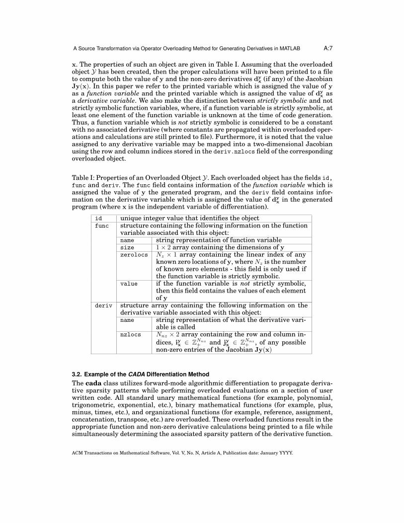
x. The properties of such an object are given in Table I. Assuming that the overloadedobject Y has been created, then the proper calculations will have been printed to a fileto compute both the value of y and the non-zero derivatives dy
x (if any) of the JacobianJy(x). In this paper we refer to the printed variable which is assigned the value of yas a function variable and the printed variable which is assigned the value of dy
x asa derivative variable. We also make the distinction between strictly symbolic and notstrictly symbolic function variables, where, if a function variable is strictly symbolic, atleast one element of the function variable is unknown at the time of code generation.Thus, a function variable which is not strictly symbolic is considered to be a constantwith no associated derivative (where constants are propagated within overloaded oper-ations and calculations are still printed to file). Furthermore, it is noted that the valueassigned to any derivative variable may be mapped into a two-dimensional Jacobianusing the row and column indices stored in the deriv.nzlocs field of the correspondingoverloaded object.
Table I: Properties of an Overloaded Object Y. Each overloaded object has the fields id,func and deriv. The func field contains information of the function variable which isassigned the value of y the generated program, and the deriv field contains infor-mation on the derivative variable which is assigned the value of dy
x in the generatedprogram (where x is the independent variable of differentiation).
id unique integer value that identifies the objectfunc structure containing the following information on the function
variable associated with this object:name string representation of function variablesize 1× 2 array containing the dimensions of yzerolocs Nz × 1 array containing the linear index of any
known zero locations of y, where Nz is the numberof known zero elements - this field is only used ifthe function variable is strictly symbolic.
value if the function variable is not strictly symbolic,then this field contains the values of each elementof y
deriv structure array containing the following information on thederivative variable associated with this object:name string representation of what the derivative vari-
able is callednzlocs Nnz × 2 array containing the row and column in-
dices, iyx ∈ ZNnz
+ and jyx ∈ ZNnz
+ , of any possiblenon-zero entries of the Jacobian Jy(x)
3.2. Example of the CADA Differentiation Method
The cada class utilizes forward-mode algorithmic differentiation to propagate deriva-tive sparsity patterns while performing overloaded evaluations on a section of userwritten code. All standard unary mathematical functions (for example, polynomial,trigonometric, exponential, etc.), binary mathematical functions (for example, plus,minus, times, etc.), and organizational functions (for example, reference, assignment,concatenation, transpose, etc.) are overloaded. These overloaded functions result in theappropriate function and non-zero derivative calculations being printed to a file whilesimultaneously determining the associated sparsity pattern of the derivative function.
ACM Transactions on Mathematical Software, Vol. V, No. N, Article A, Publication date: January YYYY.

A:8 M. J. Weinstein, and A. V. Rao
In this section the CADA differentiation method is explained by considering a MAT-LAB function such that x ∈ R
n is the input and is the variable of differentiation. Letv(x) ∈ R
m contain Nnz ≤ m × n non-zero elements in the Jacobian, Jv(x), and letivx ∈ R
Nnz and jvx ∈ RNnz be the row and column indices, respectively, correspond-
ing to the non-zero elements of Jv(x). Furthermore, let dvx ∈ R
Nnz be a vector of thenon-zero elements of Jv(x). Assuming no zero function locations are known in v, thecada instance, V, would posses the following relevant properties: (i) func.name=’v.f’;(ii) func.size=[m 1]; (iii) deriv.name=’v.dx’; and (iv) deriv.nzlocs=[ivx jvx]. It is as-sumed that, since the object V has been created, the function variable, v.f, and thederivative variable, v.dx, have been printed to a file in such a manner that, upon eval-uation, v.f and v.dx will be assigned the numeric values of v and dv
x, respectively.Suppose now that the unary array operation g : R
m → Rm (e.g. sin, sqrt, etc.) is
encountered during the evaluation of the MATLAB function code. If we consider thefunction w = g(v(x)), it can easily be seen that Jw(x) and Jv(x) will contain possiblenon-zero elements in the same locations. Additionally, the non-zero derivative valuesdwx may be calculated as
dwx (k) = g′(v[ivx(k)])d
vx(k), (k = 1 . . . Nnz), (5)
where g′(·) is the derivative of g(·) with respect to the argument of the function g. Inthe file that is being created, the derivative variable, w.dx, would be written as follows.Assume that the index ivx is printed to a file such that it will be assigned to the vari-able findex within the derivative program. Then the derivative computation wouldbe written as w.dx = dg(v.f(findex)).*v.dx, and the function computation wouldsimply be written as w.f = g(v.f), where dg(·) and g(·) represent the MATLAB op-erations corresponding to g′(·) and g(·), respectively. The resulting overloaded object,W, would then have the same properties as V with the exception of id, func.name, andderiv.name. Here we emphasize that, in the above example, the derivative calculationis only valid for a vector, v, whose non-zero elements of Jv(x) lie in the row locationsdefined by ivx, and that the values of ivx and m are known at the time of the overloadedoperation.
3.3. Motivation for a New Method to Generate Derivative Source Code
The aforementioned discussion identifies the fact that the CADA method as developedin Patterson et al. [2013] may be used to transform a mathematical program contain-ing a simple basic block into a derivative program, which, when executed in MATLAB,will compute the non-zero derivatives of a fixed input size version of the original pro-gram. The method may also be applied to programs containing unrollable loops, where,if evaluated on cada objects, the resulting derivative code would contain an unrolledrepresentation of the loop. Function programs containing indeterminable conditionalstatements (that is, conditional statements which are dependent upon strictly sym-bolic objects), however, cannot be evaluated on instances of the cada class as multiplebranches may be possible. The remainder of this paper is focused on developing themethods to allow for the application of the cada class to differentiate function pro-grams containing indeterminable conditional statements and loops, where the flowcontrol of the originating program is preserved in the derivative program.
4. OVERMAPS AND UNIONS
Before proceeding to the description of the method, it is important to describe anovermap and a union, both which are integral parts of the method itself. Specifically,due to the nature of conditional blocks and loop statements, it is often the case thatdifferent assignment objects may be written to the same variable, where the deter-mination of which object is assigned depends upon which conditional branch is taken
ACM Transactions on Mathematical Software, Vol. V, No. N, Article A, Publication date: January YYYY.
A Source Transformation via Operator Overloading Method for Generating Derivatives in MATLAB A:9
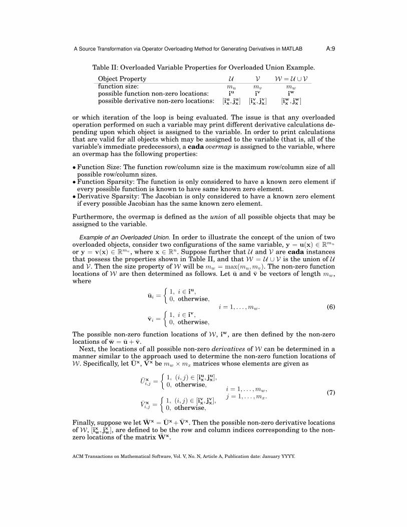
Table II: Overloaded Variable Properties for Overloaded Union Example.
Object Property U V W = U ∪ Vfunction size: mu mv mw
possible function non-zero locations: iu iv iw
possible derivative non-zero locations: [iux, jux] [ivx, j
vx] [iwx , jwx ]
or which iteration of the loop is being evaluated. The issue is that any overloadedoperation performed on such a variable may print different derivative calculations de-pending upon which object is assigned to the variable. In order to print calculationsthat are valid for all objects which may be assigned to the variable (that is, all of thevariable’s immediate predecessors), a cada overmap is assigned to the variable, wherean overmap has the following properties:
• Function Size: The function row/column size is the maximum row/column size of allpossible row/column sizes.
• Function Sparsity: The function is only considered to have a known zero element ifevery possible function is known to have same known zero element.
• Derivative Sparsity: The Jacobian is only considered to have a known zero elementif every possible Jacobian has the same known zero element.
Furthermore, the overmap is defined as the union of all possible objects that may beassigned to the variable.
Example of an Overloaded Union. In order to illustrate the concept of the union of twooverloaded objects, consider two configurations of the same variable, y = u(x) ∈ R
mu
or y = v(x) ∈ Rmv , where x ∈ R
n. Suppose further that U and V are cada instancesthat possess the properties shown in Table II, and that W = U ∪ V is the union of Uand V. Then the size property of W will be mw = max(mu,mv). The non-zero functionlocations of W are then determined as follows. Let u and v be vectors of length mw,where
ui =
{
1, i ∈ iu,0, otherwise,
vi =
{
1, i ∈ iv,0, otherwise,
i = 1, . . . ,mw. (6)
The possible non-zero function locations of W, iw, are then defined by the non-zerolocations of w = u+ v.
Next, the locations of all possible non-zero derivatives of W can be determined in amanner similar to the approach used to determine the non-zero function locations ofW. Specifically, let Ux, Vx be mw ×mx matrices whose elements are given as
Uxi,j =
{
1, (i, j) ∈ [iux, jux],
0, otherwise,
V xi,j =
{
1, (i, j) ∈ [ivx, jvx],
0, otherwise,
i = 1, . . . ,mw,j = 1, . . . ,mx.
(7)
Finally, suppose we let Wx = Ux+Vx. Then the possible non-zero derivative locationsof W, [ixw, jxw], are defined to be the row and column indices corresponding to the non-zero locations of the matrix Wx.
ACM Transactions on Mathematical Software, Vol. V, No. N, Article A, Publication date: January YYYY.

A:10 M. J. Weinstein, and A. V. Rao
5. SOURCE TRANSFORMATION VIA THE OVERLOADED CADA CLASS
A new method is now described for generating derivative files of mathematical func-tions implemented in MATLAB, where the function source code may contain flow con-trol statements. Source transformation on such function programs is performed usingthe overloaded cada class together with an overmap as described in Section 4. Themethod has the feature that the resulting derivative code depends solely on the func-tions from the native MATLAB library (that is, derivative source code generated by themethod does not depend upon overloaded statements or separate run-time functions).Furthermore, the structure of the flow control statements is transcribed to the deriva-tive source code. In this section we describe in detail the various processes that areused to carry out the source transformation. An outline of the source transformationmethod is shown in Fig. 1.
User Source toIntermediate Source
Transformation1
Source CodeData
Empty ParsingEvaluation
2
OvermappingEvaluation
4
PrintingEvaluation
6
user program
user programinput data
intermediate
program
Create MappingScheme
3
Analyze LoopOrganizationalOperation Data
5
Output.mat file
Output.m file
OFS/CFS OFS/CFS/OMS
+
+
index matrix
names
stored
objects
loop
dataref/asgn
indices
index matrices (for organizational operations within loops)
Fig. 1: Source Transformation via Operator Overloading Process
From Fig. 1 it is seen that the inputs to the transformation process are the userprogram to be differentiated together with the information required to create cadainstances of the inputs to the user program. Using Fig. 1 as a guide, the source trans-formation process starts by performing a transformation of the original source code toan intermediate source code (process ①). This intermediate source code is then evalu-ated three times on cada instances. During the first evaluation (process ②), a recordof all objects and locations relative to flow control statements is built to form an objectflow structure (OFS) and a control flow structure (CFS), but no derivative calculationsare performed. Next, an object mapping scheme (OMS) is created (process ③) using theDFS and CFS obtained from the first evaluation, where the OMS is required for thesecond and third evaluations. During the second evaluation (process ④), the intermedi-ate source code is evaluated on cada instances, where each overloaded cada operationdoes not print any calculations to a file. During this second evaluation, overmaps are
ACM Transactions on Mathematical Software, Vol. V, No. N, Article A, Publication date: January YYYY.

A Source Transformation via Operator Overloading Method for Generating Derivatives in MATLAB A:11
built and are stored in global memory (shown as stored objects output of process ④)while data is collected regarding any organizational operations contained within loops(shown as loop data output of process ④). The organizational operation data is thenanalyzed to produce special derivative mapping rules for each operation (process ⑤).During the third evaluation of the intermediate source program (process ⑥), all of thedata produced from processes ②–⑤ is used to print the final derivative program toa file. In addition, a MATLAB binary file is written that contains the reference andassignment indices required for use in the derivative source code. The details of thesteps required to transform a function program containing no function/sub-functioncalls into a derivative program are given in Sections 5.1–5.6 and correspond to theprocesses ①–⑥, respectively, shown in Fig. 1. Section 5.7 then shows how the methodsdeveloped in Sections 5.1–5.6 are applied to programs containing multiple functioncalls.
5.1. User Source-to-Intermediate-Source Transformation
The first step in generating derivative source code is to perform source-to-source trans-formation on the original program to create an intermediate source code, where theintermediate source code is an augmented version of the original source code thatcontains calls to transformation routines. This initial transformation is performed viaa purely lexical analysis within MATLAB, where first the user code is parsed line byline to determine the location of any flow control keywords (that is, if, elseif, else,for, end). The code is then read again, line by line, and the intermediate program isprinted by copying sections of the user code and applying different augmentations atthe statement and flow control levels.
Figure 2 shows the transformation of a basic block in the original program, A, intothe basic block of the intermediate program, A′. At the basic block level, it is seen thateach user assignment is copied exactly from the user program to the intermediate pro-gram, but is followed by a call to the transformation routine VarAnalyzer . It is alsoseen that, after any object is written to a variable, the variable analyzer is providedthe assignment object, the string of code whose evaluation resulted in the assignmentobject, the name of the variable to which the object was written, and a flag statingwhether or not the assignment was an array subscript assignment. After each assign-ment object is sent to the VarAnalyzer , the corresponding variable is immediatelyrewritten on the output of the VarAnalyzer routine. By sending all assigned variablesto the variable analyzer it is possible to distinguish between assignment objects andintermediate objects and determine the names of the variables to which each assign-ment object is written. Additionally, by rewriting the variables on the output of thevariable analyzer, full control over the evaluating workspace is given to the transfor-mation routines. Consequently, all variables (and any operations performed on them)are forced to be overloaded.
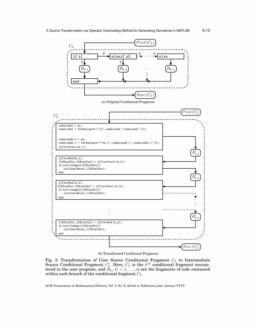
Figure 3 shows the transformation of the kth conditional fragment encountered inthe original program to a transformed conditional fragment in the intermediate pro-gram. In the original conditional fragment, Ck, each branch contains the code fragmentBk,i (i = 1, . . . , n), where the determination of which branch is evaluated depends uponthe logical values of the statements s1,s2,· · · ,sn-1. In the transformed conditionalfragment, it is seen that no flow control surrounds any of the branches. Instead, allconditional variables are evaluated and sent to the IfInitialize transformation rou-tine. Then the transformed branch fragments B′
k,1, · · · , B′
k,n are evaluated in a linearmanner, with a call to the transformation routines IfIterStart and IfIterEnd be-fore and after the evaluation of each branch fragment. By replacing all conditionalstatements with transformation routines, the control of the flow is given to the trans-
ACM Transactions on Mathematical Software, Vol. V, No. N, Article A, Publication date: January YYYY.
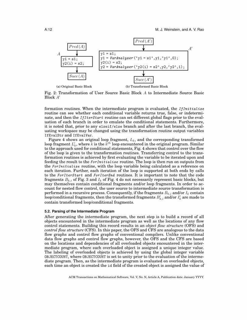
A:12 M. J. Weinstein, and A. V. Rao
y1 = s1;y2(i) = s2;
Pred (A)
Succ (A)
A
(a) Original Basic Block
y1 = s1;y1 = VarAnalyzer (‘y1 = s1’,y1,‘y1’,0);y2(i) = s2;y2 = VarAnalyzer (‘y2(i) = s2’,y2,‘y2’,1);
Pred (A′)
Succ (A′)
A′
(b) Transformed Basic Block
Fig. 2: Transformation of User Source Basic Block A to Intermediate Source BasicBlock A′
formation routines. When the intermediate program is evaluated, the IfInitialize
routine can see whether each conditional variable returns true, false, or indetermi-nate, and then the IfIterStart routine can set different global flags prior to the eval-uation of each branch in order to emulate the conditional statements. Furthermore,it is noted that, prior to any elseif/else branch and after the last branch, the eval-uating workspace may be changed using the transformation routine output variablesIfEvalStr and IfEvalVar.
Figure 4 shows an original loop fragment, Lk, and the corresponding transformedloop fragment L′
k, where k is the kth loop encountered in the original program. Similarto the approach used for conditional statements, Fig. 4 shows that control over the flowof the loop is given to the transformation routines. Transferring control to the trans-formation routines is achieved by first evaluating the variable to be iterated upon andfeeding the result to the ForInitialize routine. The loop is then run on outputs fromthe ForInitialize routine, with the loop variable being calculated as a reference oneach iteration. Further, each iteration of the loop is supported at both ends by callsto the ForIterStart and ForIterEnd routines. It is important to note that the codefragments Bk,i of Fig. 3 and Ik of Fig. 4 do not necessarily represent basic blocks, butmay themselves contain conditional fragments and/or loop fragments. In order to ac-count for nested flow control, the user source to intermediate source transformation isperformed in a recursive process. Consequently, if the fragments Bk,i and/or Ik containloop/conditional fragments, then the transformed fragments B′
k,i and/or I ′k are made tocontain transformed loop/conditional fragments.
5.2. Parsing of the Intermediate Program
After generating the intermediate program, the next step is to build a record of allobjects encountered in the intermediate program as well as the locations of any flowcontrol statements. Building this record results in an object flow structure (OFS) andcontrol flow structure (CFS). In this paper, the OFS and CFS are analogous to the dataflow graphs and control flow graphs of conventional compilers. Unlike conventionaldata flow graphs and control flow graphs, however, the OFS and the CFS are basedon the locations and dependencies of all overloaded objects encountered in the inter-mediate program, where each overloaded object is assigned a unique integer value.The labeling of overloaded objects is achieved by using the global integer variableOBJECTCOUNT, where OBJECTCOUNT is set to unity prior to the evaluation of the interme-diate program. Then, as the intermediate program is evaluated on overloaded objects,each time an object is created the id field of the created object is assigned the value of
ACM Transactions on Mathematical Software, Vol. V, No. N, Article A, Publication date: January YYYY.
A Source Transformation via Operator Overloading Method for Generating Derivatives in MATLAB A:13
if s1 elseif s2 · · · elseF F F
Bk,1 Bk,2 · · · Bk,n
T T
Pred (Ck)
end
Succ (Ck)
Ck
(a) Original Conditional Fragment
cadacond1 = s1;cadacond1 = VarAnalyzer (‘s1’,cadacond1,‘cadacond1’,0);
...cadacondn-1 = sn;cadacondn-1 = VarAnalyzer (‘sn-1’,cadacondn-1,‘cadacondn-1’,0);
IfIterStart (k,1);
IfIterEnd (k,1);[IfEvalStr,IfEvalVar] = IfIterStart (k,2);if not(isempty(IfEvalStr))
cellfun(@eval,(IfEvalStr);end
IfIterEnd (k,2);[IfEvalStr,IfEvalVar] = IfIterStart (k,3);if not(isempty(IfEvalStr))
cellfun(@eval,(IfEvalStr);
end
...
[IfEvalStr,IfEvalVar] = IfIterEnd (k,n);if not(isempty(IfEvalStr))
cellfun(@eval,(IfEvalStr);
end
B′
k,1
B′
k,2
...
B′
k,n
Pred (C ′
k)
Succ (C ′
k)
C ′
k
(b) Transformed Conditional Fragment
Fig. 3: Transformation of User Source Conditional Fragment Ck to IntermediateSource Conditional Fragment C ′
k. Here, Ck is the kth conditional fragment encoun-tered in the user program, and Bk,i (i = 1, . . . , n) are the fragments of code containedwithin each branch of the conditional fragment Ck.
ACM Transactions on Mathematical Software, Vol. V, No. N, Article A, Publication date: January YYYY.

A:14 M. J. Weinstein, and A. V. Rao
for i = sf
Ik
end
Pred (Lk)
Succ (Lk)
Lk
(a) Original LoopFragment
cadaLoopVar_k = sf;cadaLoopVar_k = ...
VarAnalyzer (‘sf’,cadaLoopVar_k,‘cadaLoopVar_k’,0);[adigatorForVar_k, ForEvalStr, ForEvalVar] = ...
ForInitialize (k,cadaLoopVar_k);if not(isempty(ForEvalStr))
cellfun(@eval,ForEvalStr)
end
for adigatorForVar_k_i = adigatorForVar_k;cadaForCount_k = ForIterStart (k,adigatorForVar_k_i);i = cadaLoopVar_k(:,cadaForCount_k);
i = VarAnalyzer (‘cadaLoopVar_k(:,cadaForCount_k)’,i,‘i’,0);
I ′k
[ForEvalStr, ForEvalVar] = ...ForIterEnd (k,adigatorForVar_k_i);
end
if not(isempty(ForEvalStr))cellfun(@eval,ForEvalStr)
end
Pred (L′
k)
Succ (L′
k)
L′
k
(b) Transformed Loop Fragment
Fig. 4: Transformation of User Source Loop Fragment Lk to Intermediate Source LoopFragment L′
k. The quantity Lk refers to the kth loop fragment encountered in the userprogram and Ik is the fragment of code contained within the loop.
OBJECTCOUNT, and OBJECTCOUNT is incremented. Here it is noted that if an object takeson the id field equal to i on one evaluation of the intermediate program, then thatobject will take on the id field equal to i on any evaluation of the intermediate pro-gram. Furthermore, if a loop is to be evaluated for multiple iterations, then the valueof OBJECTCOUNT prior to the first iteration is saved, and OBJECTCOUNT is set to the savedvalue prior to the evaluation of any iteration of the loop. By resetting OBJECTCOUNT atthe start of each loop iteration, we ensure that the id assigned to all objects within aloop are iteration independent.
Because it is required to know the OFS and CFS prior to performing any derivativeoperations, the OFS and CFS are built by evaluating the intermediate program ona set of empty overloaded objects. During this evaluation, no function or derivativeproperties are built. Instead, only the id field of each object is assigned and the OFSand CFS are built. Using the unique id assigned to each object, the OFS is built asfollows:
ACM Transactions on Mathematical Software, Vol. V, No. N, Article A, Publication date: January YYYY.
A Source Transformation via Operator Overloading Method for Generating Derivatives in MATLAB A:15
• Whenever an operation is performed on an object O to create a new object, P, werecord that the O.idth object was last used to create the P.idth object. Thus, after theentire program has been evaluated, the location (relative to all other created objects)of the last operation performed on O is known.
• If an object O is written to a variable, v, it is recorded that the O.idth object waswritten to a variable with the name ‘v’. Furthermore, it is noted if the object O wasthe result of an array subscript assignment or not.
Similarly, the CFS is built based off of the OBJECTCOUNT in the following manner:
• Before and immediately after the evaluation of each branch of each conditional frag-ment, the value of OBJECTCOUNT is recorded. Using these two values, it can be deter-mined which objects are created within each branch (and subsequently which vari-ables are written, given the OFS).
• Before and immediately after the evaluation of a single iteration of each for loop,the value of OBJECTCOUNT is recorded. Using the two recorded values it can then bedetermined which objects are created within the loop.
The OFS and CFS then contain most of the information contained in conventional dataflow graphs and control flow graphs, but are more suitable to the recursive manner inwhich flow control is handled in this paper.
5.3. Creating an Object Overmapping Scheme
Using the OFS and CFS obtained from the empty evaluation, it is then required thatan object mapping scheme (OMS) be built, where the OMS will be used in both theovermapping and printing evaluations. The OMS is used to tell the various transfor-mation routines when an overloaded union must be performed to build an overmap,where the overmapped object is being stored, and when the overmapped object mustbe written to a variable in the evaluating workspace. Similarly, the OMS must also tellthe transformation routines when an object must be saved, to where it will be saved,and when the saved object must be written to a variable in the evaluating workspace.We now look at how the OMS must be built in order to deal with both conditionalbranches and loop statements. We would like to note that while loops can contain breakand/or continue statements we do not present these cases for the sake of conciseness.
5.3.1. Conditional Statement Mapping Scheme. It is required to print conditional frag-ments to the derivative program such that different branches may be taken dependingupon numerical input values. The difficulty that arises using the cada class is that,given a conditional fragment, different branches can write different assignment objectsto the same output variable, and each of these assignment objects can contain differ-ing function and/or derivative properties. To ensure that any operations performed onthese variables after the conditional block are valid for any of the conditional branches,a conditional overmap must be assigned to all variables defined within a conditionalfragment and used later in the program (that is, the outputs of the conditional frag-ment). Given a conditional fragment C ′
k containing n branches, where each branchcontains the fragment B′
k,i (as shown in Fig. 3), the following rules are defined:
Mapping Rule 1:. If a variable y is written within C ′
k and read within Succ (C ′
k),then a single conditional overmap, Yc,o, must be created and assigned to the variabley prior to the execution of Succ (C ′
k).Mapping Rule 1.1:. For each branch fragment B′
k,i (i = 1, . . . , n) within which y
is written, the last object assigned to y within B′
k,i must belong to Yc,o.
ACM Transactions on Mathematical Software, Vol. V, No. N, Article A, Publication date: January YYYY.
A:16 M. J. Weinstein, and A. V. Rao
Mapping Rule 1.2:. If there exists a branch fragment B′
k,i within which y is not
written, or there exists no else branch, then the last object which is written toy within Pred (C ′
k) must belong to Yc,o.Mapping Rule 1.3:. If the conditional fragment C ′
k belongs to a parent condi-tional fragment C ′
j , where y belongs to a conditional overmap defined for C ′
j ,then the conditional overmap Yc,o must belong to the conditional overmap de-fined for the fragment C ′
j . The converse is not necessarily true.
Using Mapping Rule 1, it is determined for each conditional fragment which variablesrequire a conditional overmap and which assignment objects belong to which condi-tional overmaps. The second issue with evaluating transformed conditional fragmentsis that each branch is no longer being evaluated independently. Instead, each branchis evaluated in a linear manner. To force each conditional branch to be evaluated in-dependently, the following mapping rule is defined for each transformed conditionalfragment C ′
k:
Mapping Rule 2:. If a variable y is written within Pred (C ′
k), rewritten within abranch fragment B′
k,i and read within a branch fragment B′
k,j (i < j), then the lastobject written to y within Pred (C ′
k) must be saved. Furthermore, the saved objectmust be assigned to the variable y prior to the evaluation of the fragment B′
k,j .
In order to adhere to Mapping Rule 2, we use the OFS and CFS to determine theid of all objects which must be saved, where they will be saved to, and the id of theassignment objects who must be replaced with the saved objects.
5.3.2. Loop Mapping Scheme. In order to print derivative calculations within loops inthe derivative program, a single loop iteration must be evaluated on a set of overloadedinputs to the loop, where the input function sizes and/or derivative sparsity patternsmay change with each loop iteration. While simply overmapping the loop inputs willresult in a loop which is valid for all iterations, by doing so, some overloaded opera-tions within the loop may result in objects with false non-zero derivatives. Therefore,sparsity within the loop is maintained by creating both a loop overmap for each loopinput and for each assignment object created within the loop. The first mapping ruleis now given for a transformed loop L′
k of the form shown in Fig. 4.
Mapping Rule 3:. If a variable is written within I ′k, then it must belong to a loopovermap.
Mapping Rule 3.1:. If a variable y is written within Pred (L′
k), read within I ′k,and then rewritten within I ′k (that is, y is an iteration dependent input to I ′k),then the last objects written to y within Pred (L′
k) and I ′k must share the sameloop overmap. Furthermore, during the printing evaluation, the loop overmapmust be written to the variable y prior to the evaluation of I ′k.Mapping Rule 3.2:. If an assignment object belongs to a loop overmap on oneloop iteration, then it belongs to the same loop overmap on all other loop itera-tions.Mapping Rule 3.3:. If an assignment object is created within multiple nestedloops, then it still only belongs to one loop overmap.Mapping Rule 3.4:. Any assignment object which results from an array sub-script assignment belongs to the same loop overmap as the last object whichwas written to the same variable.Mapping Rule 3.5:. Any object belonging to a conditional overmap within a loopmust share the same loop overmap as all objects which belong to the conditionalovermap.
ACM Transactions on Mathematical Software, Vol. V, No. N, Article A, Publication date: January YYYY.
A Source Transformation via Operator Overloading Method for Generating Derivatives in MATLAB A:17
Using this set of rules together with the developed OFS and CFS, it is determined,for each loop L′
k, which assignment objects belong to which loop overmaps. The secondmapping rule associated with loops results from the fact that, after the loop has beenevaluated, it is no longer necessary for any active loop overmaps to exist in the eval-uating workspace. Loop overmaps are eliminated from the evaluating workspace byreplacing them with assignment objects that result from the overloaded evaluation ofall iterations of the loop. This final mapping rule is stated as follows:
Mapping Rule 4:. For any outer loop L′
k (that is, there does not exist L′
j such thatL′
k ⊂ L′
j), if a variable y is written within I ′k, and read within Succ (L′
k), then thelast object written to y within the loop during the overmapping evaluation must besaved. Furthermore, the saved object must be written to y prior to the evaluation ofSucc (L′
k) in both the overmapping and printing evaluations.
The id field of any assignment objects subject to Mapping Rule 4 are marked so thatthe assignment objects may be saved at the time of their creation and accessed at alater time.
5.4. Overmapping Evaluation
The purpose of the overmapping evaluation is to build the aforementioned conditionalovermaps and loop overmaps, as well as to collect data regarding organizational op-erations within loop statements. This overmapping evaluation is performed by eval-uating the intermediate program on overloaded cada objects, where no calculationsare printed to file, but rather only data is collected. Recall now from Mapping Rules1 and 3 that any object belonging to a conditional and/or loop overmap must be anassignment object. Additionally, all assignment objects are sent to the VarAnalyzer
routine immediately after they are created. Thus, building the conditional and loopovermaps may be achieved by performing overmapped unions within the variable an-alyzer routine. The remaining transformation routines must then control the flow ofthe program and manipulate the evaluating workspace such that the proper overmapsare built. We now describe the tasks performed by the transformation routines duringthe overmapping evaluation of conditional and loop fragments.
5.4.1. Overmapping Evaluation of Conditional Fragments. During the overmapping eval-uation of a conditional fragment, it is required to emulate the correspondingconditional statements of the original program. First, those branches on whichovermapping evaluations are performed must be determined. This determinationis made by analyzing the conditional variables given to the IfInitialize routine(cadacond1,. . . ,cadacondn-1 of Fig. 3), where each of these variables may take on avalue of true, false, or indeterminate. Any value of indeterminate implies that the vari-able may take on the value of either true or false within the derivative program. Usingthis information, it can be determined if overmapping evaluations are not to be per-formed within any of the branches. For any such branches within which overmappingevaluations are not to be performed, empty evaluations are performed in a mannersimilar to those performed in the parsing evaluation. Next, it is required that allbranches of the conditional fragment be evaluated independently (that is, we mustadhere to Mapping Rule 2). Thus, for a conditional fragment C ′
k, if a variable is writ-ten within Pred (C ′
k), rewritten within B′
k,i, and then read within B′
k,j (i < j), thenthe variable analyzer will use the developed OMS to save the last assignment objectwritten to the variable within Pred (C ′
k). The saved object may then be written to theevaluating workspace prior to the evaluation of any dependent branches using the out-puts of the IfIterStart routines corresponding to the dependent branches. Finally, inorder to ensure that any overmaps built after the conditional fragment are valid for all
ACM Transactions on Mathematical Software, Vol. V, No. N, Article A, Publication date: January YYYY.
A:18 M. J. Weinstein, and A. V. Rao
branches of the conditional fragment, all conditional overmaps associated with the con-ditional fragment must be assigned to the evaluating workspace. For some conditionalovermap, these assignments are achieved ideally within the VarAnalyzer at the timewhich the last assignment object belonging to the conditional overmap is assigned. If,however, such assignments are not possible (due to the variable being read prior to theend of the conditional fragment), then the conditional overmap may be assigned to theevaluating workspace via the outputs of the last IfIterEnd routine.
5.4.2. Overmapping Evaluation of Loops. As seen from Fig. 4, all loops in the intermediateprogram are preceded by a call to the ForInitialize routine. In the overmappingevaluation, this routine determines the size of the second dimension of the object to belooped upon, and returns adigatorForVar_k such that the loop will be evaluated as itwould be in the user program. During these loop iterations, the loop overmaps are builtand organizational operation data is collected. Here we stress that at no time duringthe overmapping evaluation are any loop overmaps active in the evaluating workspace.Thus, after the loop has been evaluated for all iterations, the objects which resultfrom the evaluation of the last iteration of the loop will be active in the evaluatingworkspace. Furthermore, on this last iteration, the VarAnalyzer routine saves anyobjects subject to Mapping Rule 4 for use in the printing evaluation.
5.5. Organizational Operations within For Loops
Consider that all organizational operations may be written as one or more references orassignments, horizontal or vertical concatenation can be written as multiple subscriptindex assignments, reshapes can be written as either a reference or a subscript indexassignment, etc. Now, consider that, given a changing function reference/assignmentindex, it is not possible in general to write the reference or assignment of a derivativevariable in terms of the changing function reference/assignment index. As a result, it isnot possible to print rolled loops in the derivative program that contain organizationaloperations simply by building overmaps.
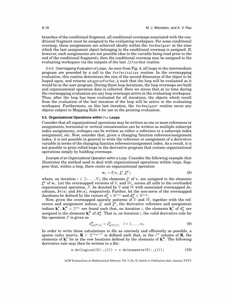
Example of an Organizational Operation within a Loop. Consider the following example thatillustrates the method used to deal with organizational operations within loops. Sup-pose that, within a loop, there exists an organizational operation
wi = f(vi, jvi , j
wi ), (8)
where, on iteration i ∈ [1, . . . , N ], the elements jvi of vi are assigned to the elementsjwi of wi. Let the overmapped versions of Vi and Wi, across all calls to the overloadedorganizational operation, F , be denoted by V and W with associated overmapped Ja-cobians, Jv(x) and Jw(x), respectively. Further, let the non-zeros of the overmappedJacobians be defined by the vectors dv
x ∈ Rnzv and dw
x ∈ Rnzw .
Now, given the overmapped sparsity patterns of V and W , together with the ref-erence and assignment indices, jvi and jwi , the derivative reference and assignmentindices k
vi , k
wi ∈ Z
mi are found such that, on iteration i, the elements kvi of dv
x areassigned to the elements k
wi of dw
x . That is, on iteration i, the valid derivative rule forthe operation F is given as
dwx[kw
i(l)] = dvx[kv
i(l)] l = 1, . . . ,mi (9)
In order to write these calculations to file as concisely and efficiently as possible, asparse index matrix, K ∈ Z
nzw×N is defined such that, in the ith column of K, theelements of k
vi lie in the row locations defined by the elements of k
wi . The following
derivative rule may then be written to a file:
w.dx(logical(K(:,i))) = v.dx(nonzeros(K(:,i))); (10)
ACM Transactions on Mathematical Software, Vol. V, No. N, Article A, Publication date: January YYYY.
A Source Transformation via Operator Overloading Method for Generating Derivatives in MATLAB A:19
Where K corresponds to the index matrix K, i is the loop iteration, and w.dx,v.dx arethe derivative variables associated with W , V .
5.5.1. Collecting and Analyzing Organizational Operation Data. As seen in the exampleabove, derivative rules for organizational operations within loops rely on index ma-trices to print valid derivative variable references and assignments. Here it is empha-sized that, given the proper index matrix, valid derivative calculations are printed tofile in the manner shown in Eq. 10 for any organizational operation contained within aloop. The aforementioned example also demonstrates that the index matrices may bebuilt given the overmapped inputs and outputs (for example, W and V), together withthe iteration dependent function reference and assignment indices (e.g. jvi and jwi ).While there exists no single operation in MATLAB which is of the form of Eq. (8), itis noted that the function reference and assignment indices may be easily determinedfor any organizational operation by collecting certain data at each call to the operationwithin a loop. Namely, for any single call to an organizational operation, any inputreference/assignment indices and function sizes of all inputs and outputs are collectedfor each iteration of a loop within which the operation is contained. Given this infor-mation, the function reference and assignment indices are then determined for eachiteration to rewrite the operation to one of the form presented in Eq. (8). In order tocollect this data, each overloaded organizational operation must have a special rou-tine written to store the required data when it is called from within a loop during theovermapping evaluations. Additionally, in the case of multiple nested loops, the datafrom each child loop must be neatly collected on each iteration of the parent loop’sForIterEnd routine. Furthermore, because it is required to obtain the overmappedversions of all inputs and outputs and it is sometimes the case that an input and/oroutput does not belong to a loop overmap, it is also sometimes the case that unionsmust be performed within the organizational operations themselves in order to buildthe required overmaps.
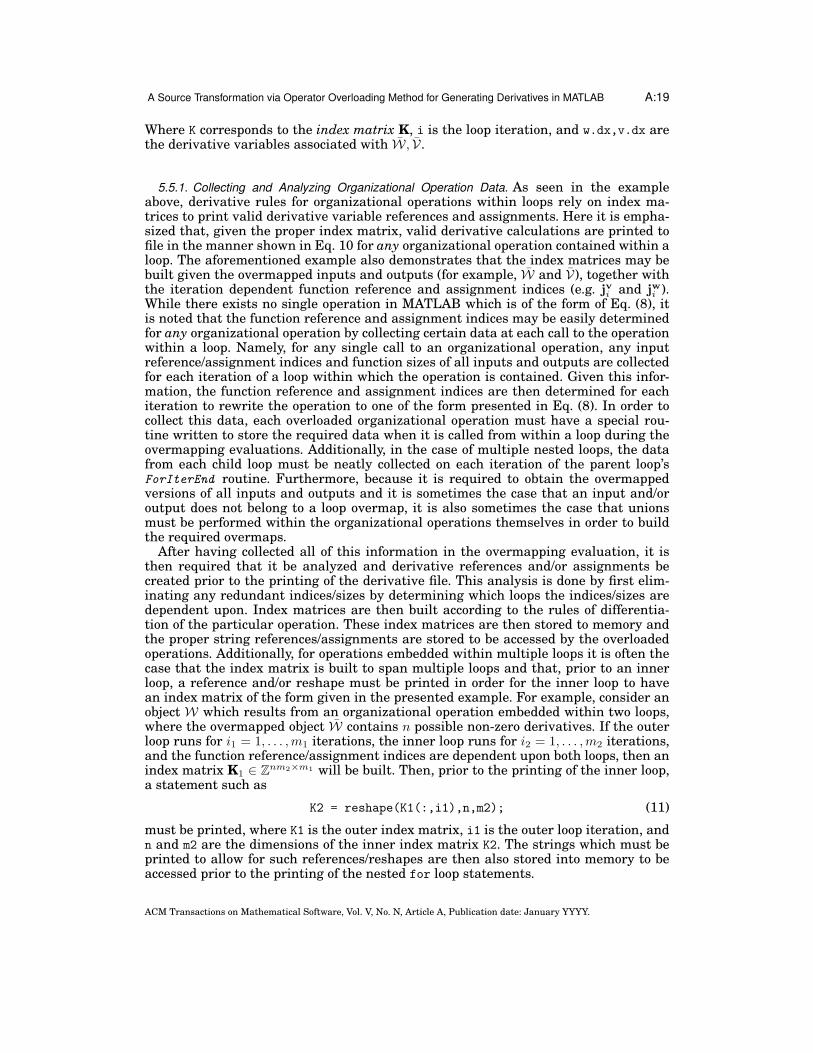
After having collected all of this information in the overmapping evaluation, it isthen required that it be analyzed and derivative references and/or assignments becreated prior to the printing of the derivative file. This analysis is done by first elim-inating any redundant indices/sizes by determining which loops the indices/sizes aredependent upon. Index matrices are then built according to the rules of differentia-tion of the particular operation. These index matrices are then stored to memory andthe proper string references/assignments are stored to be accessed by the overloadedoperations. Additionally, for operations embedded within multiple loops it is often thecase that the index matrix is built to span multiple loops and that, prior to an innerloop, a reference and/or reshape must be printed in order for the inner loop to havean index matrix of the form given in the presented example. For example, consider anobject W which results from an organizational operation embedded within two loops,where the overmapped object W contains n possible non-zero derivatives. If the outerloop runs for i1 = 1, . . . ,m1 iterations, the inner loop runs for i2 = 1, . . . ,m2 iterations,and the function reference/assignment indices are dependent upon both loops, then anindex matrix K1 ∈ Z
nm2×m1 will be built. Then, prior to the printing of the inner loop,a statement such as
K2 = reshape(K1(:,i1),n,m2); (11)
must be printed, where K1 is the outer index matrix, i1 is the outer loop iteration, andn and m2 are the dimensions of the inner index matrix K2. The strings which must beprinted to allow for such references/reshapes are then also stored into memory to beaccessed prior to the printing of the nested for loop statements.
ACM Transactions on Mathematical Software, Vol. V, No. N, Article A, Publication date: January YYYY.

A:20 M. J. Weinstein, and A. V. Rao
5.6. Printing Evaluation
During the printing evaluation we finally print the derivative code to a file by evalu-ating the intermediate program on instances of the cada class, where each overloadedoperation prints calculations to the file in the manner presented in Section 3. In orderto print if statements and for loops to the file that contains the derivative program,the transformation routines must both print flow control statements and ensure theproper overloaded objects exist in the evaluating workspace. Manipulating the evalu-ating workspace in this manner enables all overloaded operations to print calculationsthat are valid for the given flow control statements. Unlike in the overmapping evalua-tions, if the evaluating workspace is changed, then the proper re-mapping calculationsmust be printed to the derivative file such that all function variables and derivativevariables within the printed file reflect the properties of the objects within the activeevaluating workspace. We now introduce the concept of an overloaded re-map and ex-plore the various tasks performed by the transformation routines to print derivativeprograms containing both conditional and loop fragments.
5.6.1. Re-Mapping of Overloaded Objects. During the printing of the derivative program,it is often the case that an overloaded object must be written to a variable in the in-termediate program by means of the transformation routines, where the variable waspreviously written by the overloaded evaluation of a statement copied from the userprogram. Because the derivative program is simultaneously being printed as the in-termediate program is being evaluated, any time a variable is rewritten by means ofa transformation routine, the printed function and derivative variable must be madeto reflect the properties of the new object being written to the evaluating workspace.If an object O is currently assigned to a variable in the intermediate program, and atransformation routine is to assign a different object, P, to the same variable, thenthe overloaded operation which prints calculations to transform the function variableand derivative variable(s) which reflect the properties of O to those which reflect theproperties of P is referred to as the re-map of O to P. To describe this process, con-sider the case where both O and P contain derivative information with respect to aninput object X . Furthermore, let o.f and o.dx be the function variable and derivativevariable which reflect the properties of O. Here it can be assumed that, because O isactive in the evaluating workspace, the proper calculations have been printed to thederivative file to compute o.f and o.dx. If it is desired to re-map O to P such that thevariables o.f and o.dx are used to create the function variable, p.f, and derivativevariable, p.dx, which reflect the properties of P, the following steps are executed:
• Build the function variable, p.f:Re-Mapping Case 1.A:. If p.f is to have a greater row and/or column dimensionthan those of o.f, then p.f is created by appending zeros to the rows and/orcolumns of o.f.Re-Mapping Case 1.B:. If p.f is to have a lesser row and/or column dimensionthan those of o.f, then p.f is created by removing rows and/or columns from o.f.Re-Mapping Case 1.C:. If p.f is to have the same dimensions as those of o.f, thenp.f is set equal to o.f.
• Build the derivative variable, p.dx:Re-Mapping Case 2.A:. If P has more possible non-zero derivatives than O, thenp.dx is first set equal to a zero vector and then o.dx is assigned to elements ofp.dx, where the assignment index is determined by the mapping of the derivativelocations defined by O.deriv.nzlocs into those defined by P.deriv.nzlocs.Re-Mapping Case 2.B:. If P has less possible non-zero derivatives than O, thenp.dx is created by referencing off elements of o.dx, where the reference index is
ACM Transactions on Mathematical Software, Vol. V, No. N, Article A, Publication date: January YYYY.

A Source Transformation via Operator Overloading Method for Generating Derivatives in MATLAB A:21
determined by the mapping of the derivative locations defined by P.deriv.nzlocsinto those defined by O.deriv.nzlocs.Re-Mapping Case 2.C:. If P has the same number of possible non-zero derivativesas O, then p.dx is set equal to o.dx.
It is noted that, in the 1.A and 2.A cases, the object O is being re-mapped to theovermapped object P, where O belongs to P. In the 1.B and 2.B cases, the overmappedobject, O, is being re-mapped to an object P, where P belongs to O. Furthermore, there-mapping operation is only used to either map an object to an overmapped objectwhich it belongs, or to map an overmapped object to an object which belongs to theovermap.
5.6.2. Printing Evaluation of Conditional Fragments. Printing a valid conditional fragmentto the derivative program requires that the following tasks must be performed. First,it is necessary to print the conditional statements, that is, print the statements if,elseif, else, and end. Second, it is required that each conditional branch is evaluatedindependently (as was the case with the overmapping evaluation). Third, after theconditional fragment has been evaluated in the intermediate program (and printedto the derivative file), all associated conditional overmaps must be assigned to theproper variables in the intermediate program. In addition, all of the proper re-mappingcalculations must be printed to the derivative file such that when each branch of thederivative conditional fragment is evaluated it will calculate derivative variables andfunction variables that reflect the properties of the active conditional overmaps in theintermediate program. These three aforementioned tasks are now explained in furtherdetail.
The printing of the conditional branch headings is fairly straightforward due tothe manner in which all expressions following the if/elseif statements in the userprogram are written to a conditional variable in the intermediate program (as seenin Fig. 3). Thus, each IfIterStart routine may simply print the branch heading as:if cadacond1, elseif cadacond2, else and so on. As each branch of the conditionalfragment is then evaluated the overloaded cada operations will print derivative andfunction calculations to the derivative file in the manner described in Section 3. Aswas the case with the overmapping evaluations, each of the branch fragments must beevaluated independently, where this evaluation is performed in the same manner asdescribed in Section 5.4.1. Likewise, it is ensured that the evaluating workspace willcontain all associated conditional overmaps in the same manner as in the overmap-ping evaluation. Unlike the overmapping evaluation, however, conditional overmapsare not built during the printing evaluations. Instead, the conditional overmaps arestored within memory and may be accessed by the transformation routines in orderto print the proper re-mapping calculations to the derivative file. For some conditionalfragment C ′
k within which the variable y has been written, the following calculationsare required to print the function variable and derivative variable that reflect theproperties of the conditional overmap Yc,o:
• If an object Y belongs to Yc,o as a result of Mapping Rule 1.1 and is not to be operatedon from within the branch it is created, then Y is re-mapped to Yc,o from within theVarAnalyzer routine at the time of which Y is assigned to y.
• If an object Y belongs to Yc,o as a result of Mapping Rule 1.1 and is to be operated onfrom within the branch it is created, then Y is stored from within the VarAnalyzer
and the IfIterEnd routine corresponding to the branch performs the re-map of Y toYc,o.
• For each branch within which y is not written, the IfIterEnd routine accesses bothYc,o and the last object written to y within Pred (C ′
k) (where this will have been saved
ACM Transactions on Mathematical Software, Vol. V, No. N, Article A, Publication date: January YYYY.
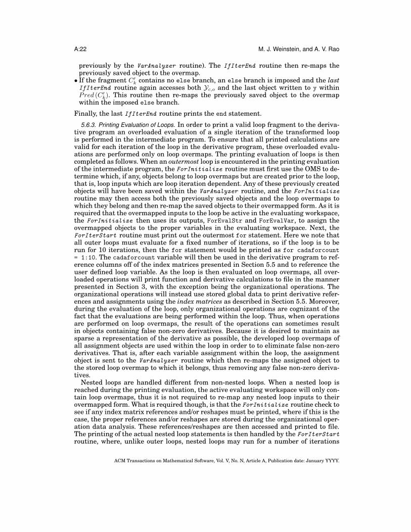
A:22 M. J. Weinstein, and A. V. Rao
previously by the VarAnalyzer routine). The IfIterEnd routine then re-maps thepreviously saved object to the overmap.
• If the fragment C ′
k contains no else branch, an else branch is imposed and the lastIfIterEnd routine again accesses both Yc,o and the last object written to y withinPred (C ′
k). This routine then re-maps the previously saved object to the overmapwithin the imposed else branch.
Finally, the last IfIterEnd routine prints the end statement.
5.6.3. Printing Evaluation of Loops. In order to print a valid loop fragment to the deriva-tive program an overloaded evaluation of a single iteration of the transformed loopis performed in the intermediate program. To ensure that all printed calculations arevalid for each iteration of the loop in the derivative program, these overloaded evalu-ations are performed only on loop overmaps. The printing evaluation of loops is thencompleted as follows. When an outermost loop is encountered in the printing evaluationof the intermediate program, the ForInitialize routine must first use the OMS to de-termine which, if any, objects belong to loop overmaps but are created prior to the loop,that is, loop inputs which are loop iteration dependent. Any of these previously createdobjects will have been saved within the VarAnalyzer routine, and the ForInitialize
routine may then access both the previously saved objects and the loop overmaps towhich they belong and then re-map the saved objects to their overmapped form. As it isrequired that the overmapped inputs to the loop be active in the evaluating workspace,the ForInitialize then uses its outputs, ForEvalStr and ForEvalVar, to assign theovermapped objects to the proper variables in the evaluating workspace. Next, theForIterStart routine must print out the outermost for statement. Here we note thatall outer loops must evaluate for a fixed number of iterations, so if the loop is to berun for 10 iterations, then the for statement would be printed as for cadaforcount= 1:10. The cadaforcount variable will then be used in the derivative program to ref-erence columns off of the index matrices presented in Section 5.5 and to reference theuser defined loop variable. As the loop is then evaluated on loop overmaps, all over-loaded operations will print function and derivative calculations to file in the mannerpresented in Section 3, with the exception being the organizational operations. Theorganizational operations will instead use stored global data to print derivative refer-ences and assignments using the index matrices as described in Section 5.5. Moreover,during the evaluation of the loop, only organizational operations are cognizant of thefact that the evaluations are being performed within the loop. Thus, when operationsare performed on loop overmaps, the result of the operations can sometimes resultin objects containing false non-zero derivatives. Because it is desired to maintain assparse a representation of the derivative as possible, the developed loop overmaps ofall assignment objects are used within the loop in order to to eliminate false non-zeroderivatives. That is, after each variable assignment within the loop, the assignmentobject is sent to the VarAnalyzer routine which then re-maps the assigned object tothe stored loop overmap to which it belongs, thus removing any false non-zero deriva-tives.
Nested loops are handled different from non-nested loops. When a nested loop isreached during the printing evaluation, the active evaluating workspace will only con-tain loop overmaps, thus it is not required to re-map any nested loop inputs to theirovermapped form. What is required though, is that the ForInitialize routine check tosee if any index matrix references and/or reshapes must be printed, where if this is thecase, the proper references and/or reshapes are stored during the organizational oper-ation data analysis. These references/reshapes are then accessed and printed to file.The printing of the actual nested loop statements is then handled by the ForIterStart
routine, where, unlike outer loops, nested loops may run for a number of iterations
ACM Transactions on Mathematical Software, Vol. V, No. N, Article A, Publication date: January YYYY.

A Source Transformation via Operator Overloading Method for Generating Derivatives in MATLAB A:23
which is dependent upon a parent loop. If it is the case that a nested loop changessize depending upon a parent loop’s iteration, then the loop statement is printed as:for cadaforcount2 = 1:K(cadaforcount1), where cadaforcount2 takes on the nestedloop iteration, cadaforcount1 is the parent loop iteration, and K is a vector containingthe sizes of the nested loop. Any evaluations performed within the nested loop are thenhandled exactly as if they were within an outer loop, and when the ForIterEnd routineof the nested loop is encountered it prints the end statement.
After the outer loop has been evaluated, the outermost ForIterEnd routine thenprints the end statement and must check to see if it needs to perform any re-mapsas a result of Mapping Rule 4. In other words, the OMS is used to determine whichvariables defined within the loop will be read after the loop (that is, which variablesare outputs of the loop). The objects that were written to these variables as a resultof the last iteration of the loop in the overmapping evaluation are saved and are nowaccessible by the ForIterEnd routine. The loop overmaps are then re-mapped to thesaved objects, and the outputs of ForIterEnd , ForEvalStr and ForEvalVar, are used toassign the saved objects to the evaluating workspace. Printing loops in this mannerensures that all calculations printed within the loop are valid for all iterations of theloop. Furthermore, this printing process ensures that any calculations printed afterthe loop are valid only for the result of the evaluation of all iterations of the loops(thus maintaining sparsity).
5.6.4. Storage of Global Data Required to Evaluate Derivative File. Because the method pre-sented in this paper is geared towards applications in which the derivative is requiredat a number of different values, it is most efficient to determine all references andassignment indices required to evaluate the derivative file only once prior to all eval-uations of the derivative file for a particular application. Thus, unlike the methodof Patterson et al. [2013], where all reference and assignment indices are embeddedwithin the derivative program itself, in the method of this paper these reference andassignment indices are written as variable names to a MATLAB binary file (which isan output of the process shown in Fig. 1). These variable names are then used withinthe derivative program itself and are recalled from global MATLAB memory. Further-more, in the case where the associated global structure is cleared, it is restored on anensuing call to the derivative program by loading the aforementioned MATLAB binaryfile associated with the derivative program. Using this aforementioned approach tokeeping track of reference and assignment indices, the overhead associated with read-ing the indices is incurred only once. Furthermore, the derivative program is printedmuch more concisely than it would have been had the indices themselves been printedto the derivative file.
5.7. Multiple User Functions
At this point, the methods have been described that transform a program containingonly a single function into a derivative program containing only a single function. Itis often the case, however, that a user program consists of multiple functions and/orsub-functions. The method of this paper handles both the cases of called functions andsub-functions in the same manner. In order to deal with programs containing mul-tiple function calls, the transformations of Fig. 5 are applied during the user sourceto intermediate source transformation phase. In the parsing phase, it is then deter-mined which functions F ′
k are called more than a single time. If a function is calledonly once, then the input and output objects are saved during the overmapping evalu-ation phase. Then, in the printing evaluation phase, when the function F ′
k is called, theFunctionInit routine returns the saved outputs and sets the adigatorFlag true, re-turning the outputs to the calling function. After the calling function has been printed,
ACM Transactions on Mathematical Software, Vol. V, No. N, Article A, Publication date: January YYYY.
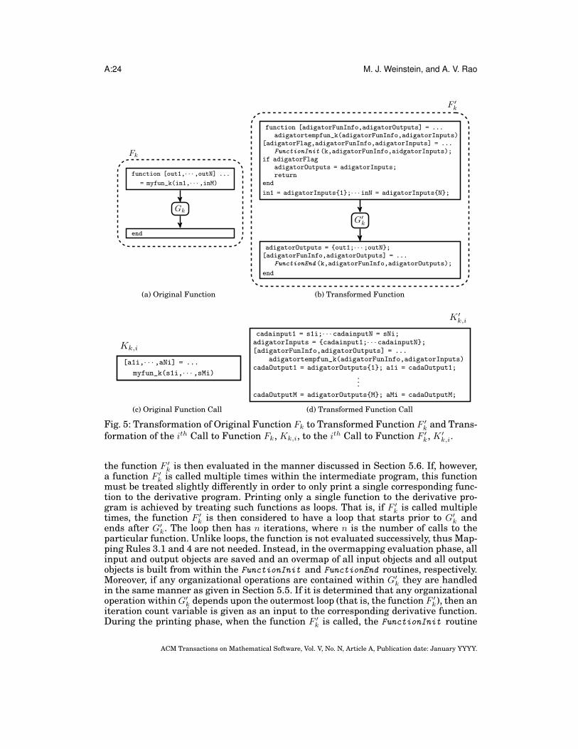
A:24 M. J. Weinstein, and A. V. Rao
function [out1,· · · ,outN] ...
= myfun_k(in1,· · · ,inM)
Gk
end
Fk
(a) Original Function
function [adigatorFunInfo,adigatorOutputs] = ...adigatortempfun_k(adigatorFunInfo,adigatorInputs)
[adigatorFlag,adigatorFunInfo,adigatorInputs] = ...FunctionInit (k,adigatorFunInfo,aidgatorInputs);
if adigatorFlagadigatorOutputs = adigatorInputs;return
end
in1 = adigatorInputs{1};· · · inN = adigatorInputs{N};
G′
k
adigatorOutputs = {out1;· · · ;outN};[adigatorFunInfo,adigatorOutputs] = ...
FunctionEnd (k,adigatorFunInfo,adigatorOutputs);
end
F ′
k
(b) Transformed Function
[a1i,· · · ,aNi] = ...
myfun_k(s1i,· · · ,sMi)
Kk,i
(c) Original Function Call
cadainput1 = s1i;· · · cadainputN = sNi;adigatorInputs = {cadainput1;· · · cadainputN};[adigatorFunInfo,adigatorOutputs] = ...
adigatortempfun_k(adigatorFunInfo,adigatorInputs)cadaOutput1 = adigatorOutputs{1}; a1i = cadaOutput1;
.
.
.
cadaOutputM = adigatorOutputs{M}; aMi = cadaOutputM;
K ′
k,i
(d) Transformed Function Call
Fig. 5: Transformation of Original Function Fk to Transformed Function F ′
k and Trans-formation of the ith Call to Function Fk, Kk,i, to the ith Call to Function F ′
k, K ′
k,i.
the function F ′
k is then evaluated in the manner discussed in Section 5.6. If, however,a function F ′
k is called multiple times within the intermediate program, this functionmust be treated slightly differently in order to only print a single corresponding func-tion to the derivative program. Printing only a single function to the derivative pro-gram is achieved by treating such functions as loops. That is, if F ′
k is called multipletimes, the function F ′
k is then considered to have a loop that starts prior to G′
k andends after G′
k. The loop then has n iterations, where n is the number of calls to theparticular function. Unlike loops, the function is not evaluated successively, thus Map-ping Rules 3.1 and 4 are not needed. Instead, in the overmapping evaluation phase, allinput and output objects are saved and an overmap of all input objects and all outputobjects is built from within the FunctionInit and FunctionEnd routines, respectively.Moreover, if any organizational operations are contained within G′
k they are handledin the same manner as given in Section 5.5. If it is determined that any organizationaloperation within G′
k depends upon the outermost loop (that is, the function F ′
k), then aniteration count variable is given as an input to the corresponding derivative function.During the printing phase, when the function F ′
k is called, the FunctionInit routine
ACM Transactions on Mathematical Software, Vol. V, No. N, Article A, Publication date: January YYYY.

A Source Transformation via Operator Overloading Method for Generating Derivatives in MATLAB A:25
re-maps the given inputs for the particular call to the overmapped inputs, prints thefunction call, re-maps the overmapped outputs to the stored outputs, and then returnsthe stored outputs. The function is then not evaluated by setting the adigatorFlag totrue. Instead, after the calling function is finished printing, the function F ′
k is thenevaluated on the overmapped inputs as if it were a for loop.
6. EXAMPLES
The method described in Section 5 (which is implemented in the software ADiGator)now is applied to four examples. The first example provides a detailed examination ofthe process that ADiGator uses to handle conditional statements. The second exampleis the well known Speelpenning problem of Speelpenning [1980] and demonstrates theability of ADiGator to handle a for loop while simultaneously providing a comparisonbetween a rolled loop and an unrolled loop. The third example is a polynomial datafitting example which contains a for loop and provides a comparison between the effi-ciency of ADiGator with the previously developed operator overloaded tool MAD [Forth2006] and the combination source transformation and operator overloading tool ADi-Mat [Bischof et al. 2003]. The fourth example is a large scale nonlinear programmingproblem (NLP) whose constraint function contains multiple levels of flow control. Thisfourth example is used to compare the efficiency of the first- and second-order deriva-tive code generated by ADiGator against the previously developed software tools INT-LAB [Rump 1999], MAD [Forth 2006], and ADiMat [Bischof et al. 2003]. Comparisonswere performed against INTLAB version 6, MAD version 1.4, and ADiMat version0.5.9. All computations were performed on an Apple Mac Pro with Mac OS-X 10.9.2(Mavericks) and a 2 × 2.4 GHz Quad-Core Intel Xeon processor with 24 GB 1066 MHzDDR3 RAM using MATLAB version R2014a.
Example 1: Conditional Statement
In this example we investigate the transformation of a user program containing a con-ditional statement into a derivative program containing the same conditional state-ment. The original user program and the transformed intermediate program is shownin Figure 6, where it is seen that the variable y is written within both the if branchand the else branch. Furthermore, because the variable y is read after the conditionalfragment, a conditional overmap, Yc,o, is required to print derivative calculations thatare valid for both the if and else branches.
Now let Yif and Yelse be the overloaded objects written to y as a result of the over-loaded evaluation of the if and else branches, respectively, in the intermediate pro-gram. Using this notation, the required conditional overmap is Yc,o = Yif∪Yelse, wherethis conditional overmap is built during the overmapping evaluation of the interme-diate program shown in Figure 6. Fixing the input to be a vector of length five, thesparsity patterns of the Jacobians defined by Yif, Yelse, and Yc,o are shown in Fig-ure 7, and the final transformed derivative program is seen in Figure 8. From Fig-ure 8, it is seen that re-mapping calculations are required from within both the ifand else branches, where these re-mapping calculations represent the mapping ofthe non-zero elements of the Jacobians shown in Figures 7a and 7b into those shownin Figure 7c. More precisely, in the if branch of the derivative program, the assign-ment indices Gator1Indices.Index4 maps the derivative variable of Yif into elements[1, 3, 4, 6, 7, 9, 10, 12, 13] of the derivative variable of Yc,o. Similarly, in the else branch ofthe derivative program, the assignment index Gator1Indices.Index8 maps the deriva-tive variable of Yelse into the [1, 2, 4, 5, 7, 8, 10, 11, 13] elements of the derivative variableof Yc,o. Thus, the evaluation of the derivative program shown in Figure 8 always pro-duces a 13 element derivative variable, z.dx, which is mapped into a Jacobian of theform shown in Figure 7c using the mapping index written to z.dx_location. Due to
ACM Transactions on Mathematical Software, Vol. V, No. N, Article A, Publication date: January YYYY.

A:26 M. J. Weinstein, and A. V. Rao
User Program Intermediate Program
function z = myfun(x)
N = 5;x1 = x(1);xN = x(N);
if x1 > xNy = x*x1;
elsey = x*xN;
end
z = sin(y);
function [adigatorFunInfo, adigatorOutputs] = ...adigatortempfunc1(adigatorFunInfo,adigatorInputs)
[adigatorFlag, adigatorFunInfo, adigatorInputs] = ...FunctionInit (1,adigatorFunInfo,adigatorInputs);
if adigatorFlag; adigatorOutputs = adigatorInputs; return; end;x = adigatorInputs{1};
N = 5;N = VarAnalyzer (‘N = 5;’,N,‘N’,0);x1 = x(1);x1 = VarAnalyzer (‘x1 = x(1);’,x1,‘x1’,0);xN = x(N);xN = VarAnalyzer (‘xN = x(N);’,xN,‘xN’,0);
% ADiGator IF Statement #1: STARTcadacond1 = x1 > xN;cadacond1 = VarAnalyzer (‘cadacond1 = x1 > xN’,cadacond1,‘cadacond1’,0);IfInitialize (1,cadacond1,[]);IfIterStart (1,1);
y = x*x1;y = VarAnalyzer (‘y = x*x1;’,y,‘y’,0);
IfIterEnd (1,1);[IfEvalStr, IfEvalVar] = IfIterStart (1,2);if not(isempty(IfEvalStr)); cellfun(@eval,IfEvalStr); end
y = x*xN;y = VarAnalyzer (‘y = x*xN;’,y,‘y’,0);
[IfEvalStr, IfEvalVar] = IfIterEnd (1,2);if not(isempty(IfEvalStr)); cellfun(@eval,IfEvalStr); end% ADiGator IF Statement #1: END
z = sin(y);z = VarAnalyzer (‘z = sin(y);’,z,‘z’,0);
adigatorOutputs = {z};[adigatorFunInfo, adigatorOutputs] = ...
FunctionEnd (1,adigatorFunInfo,adigatorOutputs);
Fig. 6: User Source-to-Intermediate Source Transformation for Example 1.
the nature of the if and else branches of the derivative program, at least 4 elementsof the derivative variable z.dx will always be identically zero, where the locations ofthe zero elements will depend upon which branch of the conditional block is taken.
d1 d2 d4 d6 d80 d3 0 0 00 0 d6 0 00 0 0 d7 00 0 0 0 d9
(a) struct(Yif.deriv)
d1 0 0 0 00 d3 0 0 00 0 d5 0 00 0 0 d7 0d2 d4 d6 d8 d9
(b) struct(Yelse.deriv)
d1 d3 d6 d9 d120 d4 0 0 00 0 d7 0 00 0 0 d10 0d2 d5 d8 d11 d13
(c) struct(Yc,o.deriv)
Fig. 7: Derivative Sparsity Patterns of Yif, Yelse, and Yc,o = Yif ∪ Yelse.
Example 2: Speelpenning Problem
This example demonstrates the transformation of a function program containing a forloop into a derivative program containing the same for loop. The function program to
ACM Transactions on Mathematical Software, Vol. V, No. N, Article A, Publication date: January YYYY.

A Source Transformation via Operator Overloading Method for Generating Derivatives in MATLAB A:27
function z = myderiv(x)global ADiGator_myderivif isempty(ADiGator_myderiv); ADiGator_LoadData(); endGator1Indices = ADiGator_myderiv.myderiv.Gator1Indices;Gator1Data = ADiGator_myderiv.myderiv.Gator1Data;% ADiGator Start Derivative Computations
FunctionInit
N.f = 5; %User Line: N = 5;x1.dx = x.dx(1); x1.f = x.f(1); %User Line: x1 = x(1);xN.dx = x.dx(5); xN.f = x.f(N.f); %User Line: xN = x(N);cadacond1 = gt(x1.f,xN.f); %User Line: cadacond1 = x1 > xN
OverloadedOperations
if cadacond1IfIterStart
cada1tempdx = x1.dx(Gator1Indices.Index1);cada1td1 = zeros(9,1);cada1td1(Gator1Indices.Index2) = x1.f.*x.dx;cada1td1(Gator1Indices.Index3) = ...
cada1td1(Gator1Indices.Index3) + x.f(:).*cada1tempdx;y.dx = cada1td1;y.f = x.f.*x1.f; %User Line: y = x*x1;
OverloadedOperation
cada1tempdx = y.dx;y.dx = zeros(13,1);y.dx(Gator1Indices.Index4,1) = cada1tempdx;
Re-MappingOperation
elseIfIterStart
cada1tempdx = xN.dx(Gator1Indices.Index5);cada1td1 = zeros(9,1);cada1td1(Gator1Indices.Index6) = xN.f.*x.dx;cada1td1(Gator1Indices.Index7) = ...
cada1td1(Gator1Indices.Index7) + x.f(:).*cada1tempdx;y.dx = cada1td1;y.f = x.f.*xN.f; %User Line: y = x*xN;
OverloadedOperations
cada1tempdx = y.dx;y.dx = zeros(13,1);y.dx(Gator1Indices.Index8,1) = cada1tempdx;
Re-MappingOperation
endIfIterEnd
cada1tf1 = y.f(Gator1Indices.Index9);z.dx = cos(cada1tf1(:)).*y.dx;z.f = sin(y.f); %User Line: z = sin(y);
OverloadedOperations
z.dx_size = [5,5];z.dx_location = Gator1Indices.Index10;end
function ADiGator_LoadData()global ADiGator_myderivADiGator_myderiv = load(‘myderiv.mat’);returnend
FunctionEnd
Fig. 8: Transformed Derivative Program for Example 1 Showing from where Each Lineis Printed.
be transformed computes the Speelpenning function [Speelpenning 1980] given as
y =N∏
i=1
xi, (12)
where Eq. (12) is implemented using a for loop as shown in Fig. 9. From Fig. 9, twomajor challenges of transforming the loop are identified. First, it is seen that the vari-able y is an input to the loop, rewritten within the loop, and read after the loop (as the
ACM Transactions on Mathematical Software, Vol. V, No. N, Article A, Publication date: January YYYY.

A:28 M. J. Weinstein, and A. V. Rao
User Program Intermediate Program
function y = SpeelFun(x)
y = 1;
for I = 1:length(x)
y = y*x(I);
end
function [adigatorFunInfo, adigatorOutputs] = ...adigatortempfun_1(adigatorFunInfo,adigatorInputs)
[flag, adigatorFunInfo, adigatorInputs] = ...FunctionInit (1,adigatorFunInfo,adigatorInputs);
if flag; adigatorOutputs = adigatorInputs; return; end;x = adigatorInputs{1};
y = 1;y = VarAnalyzer (‘y = 1;’,y,‘y’,0);
% ADiGator FOR Statement #1: STARTcadaLoopVar_1 = 1:length(x);cadaLoopVar_1 = ...
VarAnalyzer (‘cadaLoopVar_k = 1:length(x);’,cadaLoopVar_k,‘cadaLoopVar_k’,0);[adigatorForVar_1, ForEvalStr, ForEvalVar] = ForInitialize (1,cadaLoopVar_1);if not(isempty(ForEvalStr)); cellfun(@eval,ForEvalStr); endfor adigatorForVar_1_i = adigatorForVar_1
cadaForCount_1 = ForIterStart (1,adigatorForVar_1_i);I = cadaLoopVar_1(:,cadaForCount_1);I = VarAnalyzer (‘I = cadaLoopVar_1(:,cadaForCount_1);’,I,‘I’,0);y = y*x(I);y = adigatorVarAnalyzer(’y = y*x(I);’,y,’y’,0);[ForEvalStr, ForEvalVar]= ForIterEnd (1,adigatorForVar_1_i);
endif not(isempty(ForEvalStr)); cellfun(@eval,ForEvalStr); end% ADiGator FOR Statement #1: END
adigatorOutputs = {y};[adigatorFunInfo, adigatorOutputs] = ...
FunctionEnd (1,adigatorFunInfo,adigatorOutputs);
Fig. 9: User Source-to-Intermediate-Source Transformation for Speelpenning Problem.
output of the function), thus a loop overmap, Yc,o must be built to print valid derivativecalculations within the loop. Second, it is seen that the reference x(I) depends uponthe loop iteration, where the object assigned to x has possible non-zero derivatives.Thus, an index matrix, K, and an overmapped subsref output, Ro, must be built toallow for the iteration dependent derivative reference corresponding to the functionreference x(I). To further investigate, let Yi be the object written to y after the evalua-tion of the ith iteration of the loop from within the intermediate program. Furthermore,we allow Ri to be the intermediate object created as a result of the overloaded evalua-tion of x(I) within the intermediate program. The overmapped objects Yl,o and Ro arenow defined as
Yl,o =
N⋃
i=0
Yi (13)
and
Ro =N⋃
i=1
Ri, (14)
where Y0 represents the object written to y prior to the evaluation of the loop in theintermediate program. Now, as the input object, X , has a Jacobian with a diagonalsparsity pattern (which does not change), then each object Ri will have a 1×N gradientwhere the ith element is a possible non-zero. Thus, the union of all such gradients overi results in all N elements being possibly non-zero, that is, a full gradient. Within thederivative program, the reference operation must then result in a derivative variable oflength N , where on iteration i, the ith element of the derivative variable correspondingto X must be assigned to the ith element of the derivative variable corresponding toRo. This reference and assignment is done as described in Section 5.5 using the index
ACM Transactions on Mathematical Software, Vol. V, No. N, Article A, Publication date: January YYYY.

A Source Transformation via Operator Overloading Method for Generating Derivatives in MATLAB A:29
matrix K ∈ ZN×N , where
Ki,j =
{
i, i = j0, i 6= j
i = 1, . . . , Nj = 1, . . . , N
. (15)
Now, because Ri contains a possible non-zero derivative in the ith location of the gra-dient and Yi = Yi−1 ∗ Ri, Yi will contain i possible non-zero derivatives in the first ilocations. Furthermore, the union of Yi over i = 0, . . . , N results in an object Yl,o con-taining N possible non-zero derivatives (that is, a full gradient). Thus, in the derivativeprogram, the object Y0 must be re-mapped to the object Yl,o prior to the printing evalu-ation of the loop in the intermediate program. The result of the printing evaluation ofthe intermediate program for N = 10 is seen in Fig. 10. In particular, Fig. 10 shows there-mapping of the object Y0 to Yl,o immediately prior to the loop. Additionally, it is seenthat the derivative variable cada1f1dx (which results from the aforementioned refer-ence within the loop) is of length 10, where the reference and assignment of cada1f1dxdepends upon the loop iteration. This reference and assignment is made possible bythe index matrix K who is assigned to the variable Gator1Indices.Index1 within thederivative program.
Rolled vs. Unrolled Loops for Speelpenning Problem. The following important issue arisesin this example due to the fact that the loop remains rolled in the derivative code.Specifically, by imposing the overmapping scheme and maintaining a rolled loop in thederivative code, all derivative computations are forced to be dense on vectors of lengthN . If, on the other hand, the loop had been unrolled, all derivative computations oniteration i would have been performed sparsely on vectors of length i. Unrolling theloop, however, increases the size of the derivative program. To investigate the trade-offbetween between a rolled and an unrolled loop, consider for this example the Jacobian-to-function evaluation ratio, CPU(Jf)/CPU(f), for different values of N using a deriva-tive code generated with a function code that contains a rolled version of the loop and asecond derivative code generated using a function code that contains an unrolled ver-sion of the loop. The values of CPU(Jf)/CPU(f) for both the rolled and unrolled casesare shown in Table III for N = (10, 100, 1000, 10000). It is seen that unrolling the loopsresults in a more efficient derivative code, but this increase in computational efficiencycomes at the expense of generating a significantly larger derivative file. On the otherhand, it is seen that, in the worst case (N = 100), the evaluation of the rolled loop isonly about four times slower than that of the unrolled loop.
Table III: Sizes of GatorAD Generated Derivative Programs and Ratios of Jacobian-to-Function Computation time, CPU(Jf)/CPU(f), for the Rolled and Unrolled Speelpen-ning Function. File sizes were computed as the sum of the sizes of the produced .mand.mat files, and CPU(Jf)/CPU(f) were obtained by averaging the values obtainedover 1000 Jacobian and function evaluations.
CPU(Jf)/CPU(f) CPU(Jf)/CPU(f) Program Sizes (kB) Program Sizes (kB)N Ratio with Ratio with with with
Rolled Loop Unrolled Loop Rolled Loop Unrolled Loop10 223 65 1.5 2.9100 1255 297 1.9 23.31000 2522 780 6.3 370.810000 5960 3831 60.4 82170.3
ACM Transactions on Mathematical Software, Vol. V, No. N, Article A, Publication date: January YYYY.

A:30 M. J. Weinstein, and A. V. Rao
function y = SpeelDer(x)global ADiGator_SpeelDerif isempty(ADiGator_SpeelDer); ADiGator_LoadData(); endGator1Indices = ADiGator_SpeelDer.SpeelDer.Gator1Indices;Gator1Data = ADiGator_SpeelDer.SpeelDer.Gator1Data;% ADiGator Start Derivative Computations
FunctionInit
y.f = 1; %User Line: y = 1;cada1f1 = length(x.f);cadaforvar1.f = 1:cada1f1; %User Line: cadaforvar1 = 1:length(x);
OverloadedOperations
y.dx = zeros(10,1);Re-MappingOperation
for cadaforcount1 = 1:10ForInitialize
I.f = cadaforvar1.f(:,cadaforcount1);%User Line: I = cadaforvar1(:,cadaforcount1);
OverloadedOperation
cada1td1 = zeros(10,1);cada1td1(logical(Gator1Indices.Index1(:,cadaforcount1))) =...x.dx(nonzeros(Gator1Indices.Index1(:,cadaforcount1)));
cada1f1dx = cada1td1;cada1f1 = x.f(I.f);
OrganizationalOverloaded Operation
cada1td1 = cada1f1*y.dx;cada1td1 = cada1td1 + y.f*cada1f1dx;y.dx = cada1td1;y.f = y.f*cada1f1;%User Line: y = y*x(I);
OverloadedOperation
endForIterEnd
y.dx_sizy.dx_size = 10;y.dx_location = Gator1Indices.Index2;end
function GatorAD_LoadData()global GatorAD_mymax2D_derivGatorAD_mymax2D_deriv = load(‘GatorAD_mymax2D_deriv.mat’);returnend
FunctionEnd
Fig. 10: Derivative Program for Speelpenning Problem for N = 10 Showing Origin ofEach Printed Line of Code.
ACM Transactions on Mathematical Software, Vol. V, No. N, Article A, Publication date: January YYYY.
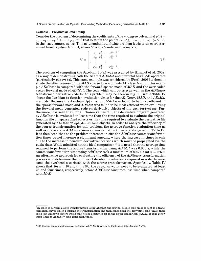
A Source Transformation via Operator Overloading Method for Generating Derivatives in MATLAB A:31
Example 3: Polynomial Data Fitting
Consider the problem of determining the coefficients of the m-degree polynomial p(x) =p1 + p2x+ p3x
2 + · · ·+ pmxm−1 that best fits the points (xi, di), (i = 1, . . . , n), (n > m),in the least squares sense. This polynomial data fitting problem leads to an overdeter-mined linear system Vp = d, where V is the Vandermonde matrix,
V =
1 x1 x21 · · · xm−1
1
1 x2 x22 · · · xm−1
2...
......
1 xn x2n · · · xm−1
n
. (16)
The problem of computing the Jacobian Jp(x) was presented by [Bischof et al. 2002]as a way of demonstrating both the AD tool ADiMat and powerful MATLAB operators(particularly, mldivide). This same example was considered by [Forth 2006] to demon-strate the effectiveness of the MAD sparse forward mode AD class fmad. In this exam-ple ADiGator is compared with the forward sparse mode of MAD and the overloadedvector forward mode of ADiMat. The code which computes p as well as the ADiGatortransformed derivative code for this problem may be seen in Fig. 11, while Table IVshows the Jacobian-to-function evaluation times for the ADiGator, MAD, and ADiMatmethods. Because the Jacobian Jp(x) is full, MAD was found to be most efficient inthe sparse forward mode and ADiMat was found to be most efficient when evaluatingthe forward mode generated code on derivative objects of the opt_derivclass. Fur-thermore, it is seen that, for all chosen values of n, the derivative program generatedby ADiGator is evaluated in less time than the time required to evaluate the originalfunction file on sparse fmad objects or the time required to evaluate the derivative filegenerated by ADiMat on opt_derivclass objects. In order to analyze the efficiency ofthe source transformation for this problem, the average function evaluation time aswell as the average ADiGator source transformation times are also given in Table IV.It is then seen that as the problem increases in size the ADiGator source transforma-tion times do not increase a significant amount, where the increase in times is onlydue to the increase in non-zero derivative locations which must be propagated via thecada class. While admitted not the ideal comparison,3 it is noted that the average timerequired to perform the source transformation using ADiMat was 0.936 s, while thesource transformation time using AdiGator took a maximum of 0.474 s (at n = 2560).An alternative approach for evaluating the efficiency of the ADiGator transformationprocess is to determine the number of Jacobian evaluations required in order to over-come the overhead associated with the source transformation. Specifically, Table IVshows that, for n = 10 and n = 2560, the Jacobian would need to be evaluated, at least26 and four times, respectively, before ADiGator consumes less time when comparedwith MAD.
3In order to perform source transformation using ADiMat, the original source code must be sent to a trans-formation server which performs the transformation and then sends back the derivative code. Thus, thereare a few unknown factors which may not be accounted for in the direct comparison of ADiMat code gener-ation times to ADiGator code generation times.
ACM Transactions on Mathematical Software, Vol. V, No. N, Article A, Publication date: January YYYY.
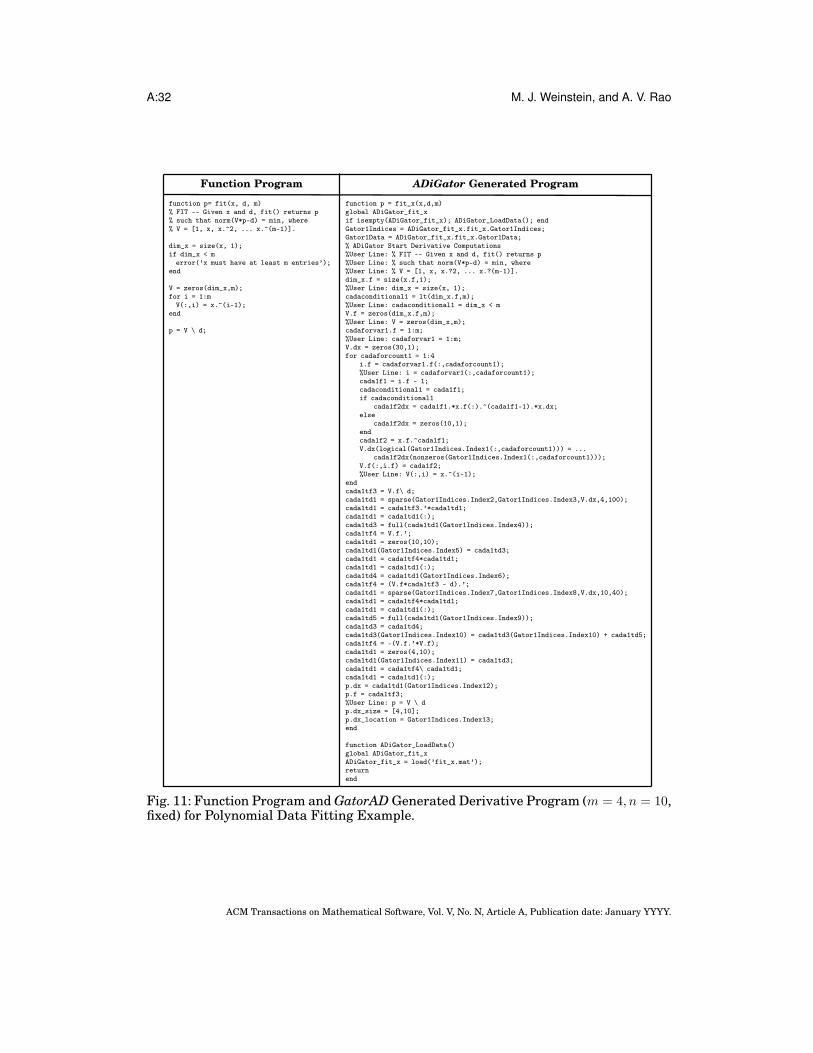
A:32 M. J. Weinstein, and A. V. Rao
Function Program ADiGator Generated Program
function p= fit(x, d, m)% FIT -- Given x and d, fit() returns p% such that norm(V*p-d) = min, where% V = [1, x, x.^2, ... x.^(m-1)].
dim_x = size(x, 1);if dim_x < merror(’x must have at least m entries’);
end
V = zeros(dim_x,m);for i = 1:mV(:,i) = x.^(i-1);
end
p = V \ d;
function p = fit_x(x,d,m)global ADiGator_fit_xif isempty(ADiGator_fit_x); ADiGator_LoadData(); endGator1Indices = ADiGator_fit_x.fit_x.Gator1Indices;Gator1Data = ADiGator_fit_x.fit_x.Gator1Data;% ADiGator Start Derivative Computations%User Line: % FIT -- Given x and d, fit() returns p%User Line: % such that norm(V*p-d) = min, where%User Line: % V = [1, x, x.?2, ... x.?(m-1)].dim_x.f = size(x.f,1);%User Line: dim_x = size(x, 1);cadaconditional1 = lt(dim_x.f,m);%User Line: cadaconditional1 = dim_x < mV.f = zeros(dim_x.f,m);%User Line: V = zeros(dim_x,m);cadaforvar1.f = 1:m;%User Line: cadaforvar1 = 1:m;V.dx = zeros(30,1);for cadaforcount1 = 1:4
i.f = cadaforvar1.f(:,cadaforcount1);%User Line: i = cadaforvar1(:,cadaforcount1);cada1f1 = i.f - 1;cadaconditional1 = cada1f1;if cadaconditional1
cada1f2dx = cada1f1.*x.f(:).^(cada1f1-1).*x.dx;else
cada1f2dx = zeros(10,1);endcada1f2 = x.f.^cada1f1;V.dx(logical(Gator1Indices.Index1(:,cadaforcount1))) = ...
cada1f2dx(nonzeros(Gator1Indices.Index1(:,cadaforcount1)));V.f(:,i.f) = cada1f2;%User Line: V(:,i) = x.^(i-1);
endcada1tf3 = V.f\ d;cada1td1 = sparse(Gator1Indices.Index2,Gator1Indices.Index3,V.dx,4,100);cada1td1 = cada1tf3.’*cada1td1;cada1td1 = cada1td1(:);cada1td3 = full(cada1td1(Gator1Indices.Index4));cada1tf4 = V.f.’;cada1td1 = zeros(10,10);cada1td1(Gator1Indices.Index5) = cada1td3;cada1td1 = cada1tf4*cada1td1;cada1td1 = cada1td1(:);cada1td4 = cada1td1(Gator1Indices.Index6);cada1tf4 = (V.f*cada1tf3 - d).’;cada1td1 = sparse(Gator1Indices.Index7,Gator1Indices.Index8,V.dx,10,40);cada1td1 = cada1tf4*cada1td1;cada1td1 = cada1td1(:);cada1td5 = full(cada1td1(Gator1Indices.Index9));cada1td3 = cada1td4;cada1td3(Gator1Indices.Index10) = cada1td3(Gator1Indices.Index10) + cada1td5;cada1tf4 = -(V.f.’*V.f);cada1td1 = zeros(4,10);cada1td1(Gator1Indices.Index11) = cada1td3;cada1td1 = cada1tf4\ cada1td1;cada1td1 = cada1td1(:);p.dx = cada1td1(Gator1Indices.Index12);p.f = cada1tf3;%User Line: p = V \ dp.dx_size = [4,10];p.dx_location = Gator1Indices.Index13;end
function ADiGator_LoadData()global ADiGator_fit_xADiGator_fit_x = load(’fit_x.mat’);returnend
Fig. 11: Function Program and GatorAD Generated Derivative Program (m = 4, n = 10,fixed) for Polynomial Data Fitting Example.
ACM Transactions on Mathematical Software, Vol. V, No. N, Article A, Publication date: January YYYY.

A Source Transformation via Operator Overloading Method for Generating Derivatives in MATLAB A:33
Table IV: Ratio of Jacobian-to-Function Computation Time, CPU(Jp(x))/CPU(p(x)),for Example 4 (m = 4) Using ADiGator, MAD, and ADiMat, Together with ADiGatorCode Generation Times and Function Evaluation Times. MAD was used in the sparseforward mode and ADiMat was used in the vector forward mode with the derivativeclass opt_derivclass. All times CPU(Jp(x)) and CPU(p(x)) were obtained by averag-ing over 100 trials and ADiGator file generation times were obtained by averaging over10 trials. It is noted that the entries for ADiMat are omitted at n = 1280 and n = 2560due to large Jacobian CPU times.
Problem Size CPU(Jp(x))/CPU(p(x)) ADiGator File CPU(p(x))n ADiGator MAD ADiMat Gen. Time (s) (ms)10 5 49 849 0.114 0.10220 7 50 1031 0.116 0.11040 7 48 1887 0.120 0.11780 7 44 4115 0.118 0.131160 9 48 23231 0.120 0.130320 11 46 103882 0.124 0.162640 17 52 604633 0.140 0.241
1280 53 139 - 0.227 0.3982560 109 300 - 0.474 0.675
ACM Transactions on Mathematical Software, Vol. V, No. N, Article A, Publication date: January YYYY.

A:34 M. J. Weinstein, and A. V. Rao
Example 4: Sparse Non-Linear Programming
Consider the following nonlinear programming problem (NLP) that arises from thediscretization of a scaled version of the optimal control problem described in [Darbyet al. 2011] using a multiple-interval formulation of the Legendre-Gauss-Radau (LGR)orthogonal collocation method as described in Patterson et al. [2013]. The NLP decisionvector z ∈ R
4N+4 is given as
z = [x1,x2,x3,u, β] , (17)
where N is a parameter that defines the number of collocation points [Garg et al. 2011;Garg et al. 2010; Garg et al. 2011; Patterson and Rao 2012], x1 ∈ R
N+1, x2 ∈ RN+1,
x3 ∈ RN+1, u ∈ R
N , and β ∈ R. Furthermore, let f : R4N+4 → R3N be defined as
fi(z) =
[
N+1∑
k=1
Di,kx1k −β
2x2i sinx3i
]
, (i = 1, . . . , N),
fN+i(z) =
[
N+1∑
k=1
Di,kx2k −β
2
(
ζ − θ
c1− c2 sinx3i
)
]
, (i = 1, . . . , N),
f2N+i(z) =
[
N+1∑
k=1
Di,kx3k −β
2
c2x2i
(ui − cosx3i)
]
, (i = 1, . . . , N),
(18)
where
ζ = ζ(T (h), h, v),θ = θ(T (h), ρ(h), h, v),
(19)
and the functions ζ, θ, T , and ρ, are evaluated at values h = x1i and v = x2i, where x1i
and x2i are the ith elements of the vectors x1 and x2, respectively. Furthermore, thequantity [Dik] ∈ R
N×(N+1) in Eq. (18) is the LGR differentiation matrix [Garg et al.2011; Garg et al. 2010; Garg et al. 2011; Patterson and Rao 2012]. It is noted thatN = NkK, where K is the number of mesh intervals that the problem is divided viausing the multiple-interval LGR collocation method. The objective of the NLP whicharises from the discretization is to minimize the cost function
J = β (20)
subject to the nonlinear algebraic constraints
f(x) = 0 (21)
and the simple bounds on the decision variables
zmin ≤ z ≤ zmax, (22)
where
x1 = b1 , xN+1 = b2,xN+2 = b3 , x2N+2 = b4x2N+3 = b5 , x3N+3 = b6.
(23)
A key aspect of this example is the modification of the functions T (h) and ρ(h) fromsmooth functions (as used in Darby et al. [2011]) to the following piecewise continuousfunctions taken from Ref. NOAA [1976]:
ρ(h) = c3p(h)
T (h)(24)
ACM Transactions on Mathematical Software, Vol. V, No. N, Article A, Publication date: January YYYY.

A Source Transformation via Operator Overloading Method for Generating Derivatives in MATLAB A:35
Table V: Constants and Parameters for Example 4.
c1 3.9240× 10² c2 1.6818× 10⁴ c3 8.6138× 101
c4 2.8814× 10² c5 6.4900× 100 c6 4.0519× 10⁹
c7 2.8808× 10² c8 5.2560× 100 c9 2.1664× 10²
c10 9.0600× 10⁸ c11 1.7300× 100 c12 1.5700× 10⁻¹
c13 6.0000× 10⁻⁵ c14 4.00936× 100 c15 2.2000× 100
b1 0 b2 2.0000× 10 b3 2.6000× 10b4 5.9000× 100 b5 0 b6 0
where
(T (h), p(h)) =
(
c4 − c5h, c6
[
T (h)c7
]c8)
, h < 11,
(c9, c10ec11−c12h) , otherwise.
(25)
In the implementation considered in this example, Eq. (25) is represented by a con-ditional statement nested within a for loop. Figure 12 shows the MATLAB code thatcomputes the function f(z), where it is seen that the source code contains multipleloops, an indeterminate conditional statement (nested within a loop) and a loop iter-ation dependent conditional statement. Table V shows the constants and parametersused in this example.
In order to solve the NLP of Eqs. (20)–(22), typically either a first-derivative (quasi-Newton) or a second-derivative (Newton) NLP solver is used. In a first-derivativesolver the objective gradient and constraint Jacobian, Jf(z), are used together with adense quasi-Newton approximation of the Lagrangian Hessian. In a second-derivativesolver, the objective gradient and constraint Jacobian are used together with the Hes-sian of the NLP Lagrangian, where in this case the Lagrangian is given by
L = β + λT f(z). (26)
In this example we now concern ourselves with the computation of both the constraintJacobian, Jf(z), and the Lagrangian Hessian, HL(z). Moreover, the efficiencies withwhich the method of this paper generates the constraint Jacobian and Lagrangian Hes-sian source code is presented along with the computational efficiency of the resultingderivative code. In order to analyze the performance of the method as the aforemen-tioned NLP increases in size, the number of LGR points in each mesh interval is setto four (that is, Nk = 4) and the number of mesh intervals, K, is varied. Thus, in thisexample, the total number of LGR points is always N = 4K. Finally, the comparativeperformance of the method developed in this paper against the well known MATLABautomatic differentiation tools INTLAB, MAD, and ADiMat is provided.
Table VI shows the ratio of the constraint Jacobian evaluation time to constraintfunction evaluation time, CPU(Jf )/CPU(f ), using the derivative code generated byADiGator alongside the values of CPU(Jf )/CPU(f ) using ADiMat, INTLAB, and MAD,where ADiMat is used in both of its non-overloaded (scalar and vector) modes whilebeing supplied the compressed seed matrix S ∈ R
4N+4×5, while MAD was used in thecompressed mode with the same seed matrix. Also, it is noted that the compressedseed matrix, S, has a column dimension 1 + max(Nk) = 5, for any K used in this ex-ample. From Table VI it is seen that the Jacobian is computed in a smaller amount oftime using the ADiGator generated code than any of the other methods. Moreover, itis seen that, for all values of K used, the time required to evaluate the derivative codegenerated by ADiGator (and produce the entire Jacobian) is slightly greater than the
ACM Transactions on Mathematical Software, Vol. V, No. N, Article A, Publication date: January YYYY.
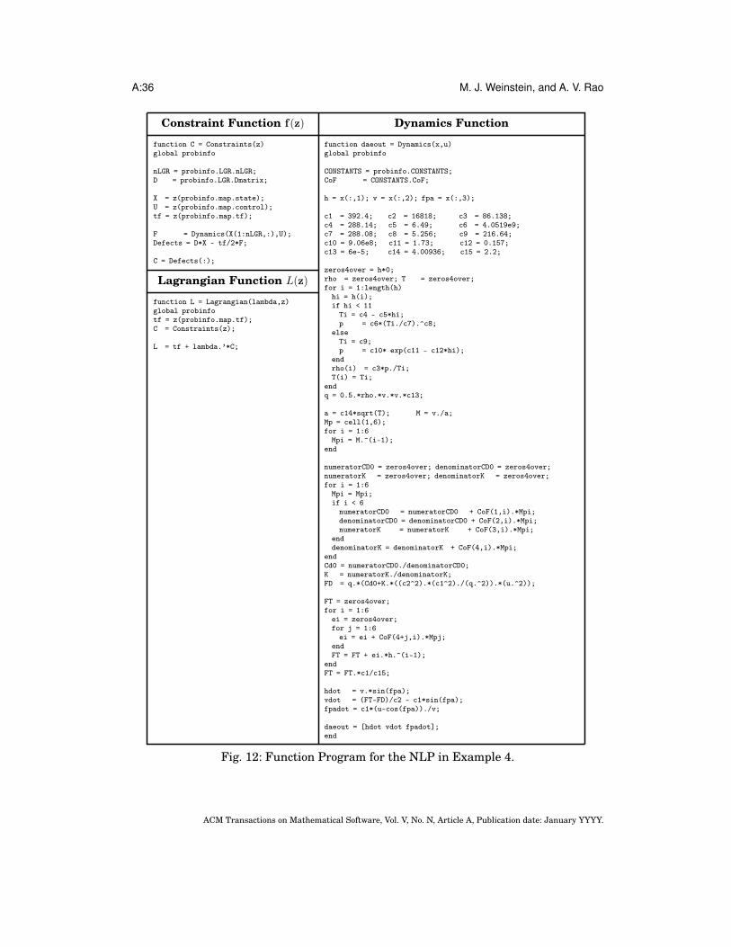
A:36 M. J. Weinstein, and A. V. Rao
Constraint Function f(z) Dynamics Function
function C = Constraints(z)global probinfo
nLGR = probinfo.LGR.nLGR;D = probinfo.LGR.Dmatrix;
X = z(probinfo.map.state);U = z(probinfo.map.control);tf = z(probinfo.map.tf);
F = Dynamics(X(1:nLGR,:),U);Defects = D*X - tf/2*F;
C = Defects(:);
function daeout = Dynamics(x,u)global probinfo
CONSTANTS = probinfo.CONSTANTS;CoF = CONSTANTS.CoF;
h = x(:,1); v = x(:,2); fpa = x(:,3);
c1 = 392.4; c2 = 16818; c3 = 86.138;c4 = 288.14; c5 = 6.49; c6 = 4.0519e9;c7 = 288.08; c8 = 5.256; c9 = 216.64;c10 = 9.06e8; c11 = 1.73; c12 = 0.157;c13 = 6e-5; c14 = 4.00936; c15 = 2.2;
zeros4over = h*0;rho = zeros4over; T = zeros4over;for i = 1:length(h)hi = h(i);if hi < 11Ti = c4 - c5*hi;p = c6*(Ti./c7).^c8;
elseTi = c9;p = c10* exp(c11 - c12*hi);
endrho(i) = c3*p./Ti;T(i) = Ti;
endq = 0.5.*rho.*v.*v.*c13;
a = c14*sqrt(T); M = v./a;Mp = cell(1,6);for i = 1:6Mpi = M.^(i-1);
end
numeratorCD0 = zeros4over; denominatorCD0 = zeros4over;numeratorK = zeros4over; denominatorK = zeros4over;for i = 1:6Mpi = Mpi;if i < 6numeratorCD0 = numeratorCD0 + CoF(1,i).*Mpi;denominatorCD0 = denominatorCD0 + CoF(2,i).*Mpi;numeratorK = numeratorK + CoF(3,i).*Mpi;
enddenominatorK = denominatorK + CoF(4,i).*Mpi;
endCd0 = numeratorCD0./denominatorCD0;K = numeratorK./denominatorK;FD = q.*(Cd0+K.*((c2^2).*(c1^2)./(q.^2)).*(u.^2));
FT = zeros4over;for i = 1:6ei = zeros4over;for j = 1:6ei = ei + CoF(4+j,i).*Mpj;
endFT = FT + ei.*h.^(i-1);
endFT = FT.*c1/c15;
hdot = v.*sin(fpa);vdot = (FT-FD)/c2 - c1*sin(fpa);fpadot = c1*(u-cos(fpa))./v;
daeout = [hdot vdot fpadot];end
Lagrangian Function L(z)
function L = Lagrangian(lambda,z)global probinfotf = z(probinfo.map.tf);C = Constraints(z);
L = tf + lambda.’*C;
Fig. 12: Function Program for the NLP in Example 4.
ACM Transactions on Mathematical Software, Vol. V, No. N, Article A, Publication date: January YYYY.

A Source Transformation via Operator Overloading Method for Generating Derivatives in MATLAB A:37
time required to evaluate the derivative code generated by ADiMat in the scalar mode(and produce a single column of the compressed Jacobian).
Table VI: Ratio of Jacobian-to-Function Computation Time, CPU(Jf)/CPU(f), for Ex-ample 4 Using ADiGator, ADiMat, INTLAB and MAD. ADiMat was supplied the com-pressed seed matrix in both the scalar forward and non-overloaded vector forwardmodes and MAD was used in the compressed forward mode and the sparse forwardmode. All times CPU(Jf) and CPU(f) were obtained by taking the average over 100Jacobian and function evaluations.
NLP Size CPU(Jf(z))/CPU(f(z))ADiGator ADiMat ADiMat INTLAB MAD MAD
K N = 4K (scalar) (vector) (comp) (sparse)4 16 17 79 142 149 188 1868 32 21 93 210 220 275 27616 64 29 116 322 332 417 42132 128 41 151 502 511 636 650
Table VII now shows the ratio of Lagrangian Hessian evaluation time to Lagrangianfunction evalaution, CPU(HL)/CPU(L), using the derivative code generated by ADi-Gator alongside the values of CPU(HL)/CPU(L) using ADiMat, INTLAB and MAD.Unlike the constraint Jacobian, the Lagrangian Hessian is incompressible and as suchMAD is only used in the sparse forward over forward mode. The non-overloaded modesof ADiMat may not be used to compute the Lagrangian Hessian as only the diagonalelements of Hessians may be computed via strip-mining and, currently, source trans-formation may not be recursively called on ADiMat generated code produced for thenon-overloaded vector mode (as it is written in terms of ADiMat specific run-time func-tions). The computation of the Lagrangian Hessian using ADiMat was thus found tobe most efficient when evaluating a Lagrangian gradient code generated in the re-verse mode on a set of overloaded objects (the default mode of the ADiMat functionadmHessian). From Table VII it is again seen that the ADiGator generated code is moreefficient than the other methods. It is also seen, however, that this efficiency appearsto dissipate (when compared to INTLAB) as the NLP grows in size.
Table VII: Ratio of Hessian-to-Function Computation Time, CPU(HL(z))/CPU(f(z)),for Example 4 Using ADiGator, ADiMat, INTLAB and MAD. MAD was used in thesparse forward over forward mode and ADiMat was used in the operator overloadingover reverse source transformation mode. All times CPU(HL(z)) and CPU(L(z)) wereobtained by taking the average over 100 Jacobian and function evaluations.
NLP Size CPU(HL(z))/CPU(L(z))K N = 4K ADiGator INTLAB MAD ADiMat
4 16 32 198 708 52028 32 48 270 1132 959016 64 93 382 2287 2120632 128 330 573 6879 55697
To this point in the example it has been shown that the Jacobian and Hessian pro-grams generated by the method of this paper are efficient when compared with otherMATLAB AD tools. The expense of the code generation then comes into question. Thetime required to generate the constraint Jacobian and Lagrangian Hessian derivative
ACM Transactions on Mathematical Software, Vol. V, No. N, Article A, Publication date: January YYYY.

A:38 M. J. Weinstein, and A. V. Rao
files using ADiGator are now given in Table VIII as well as the constraint and La-grangian function evaluation times. Unlike the previous example, there are two rea-sons for the increase in derivative file generation times seen in Table VIII. Namely,the increase in time is both due to an increase in the number of propagated non-zeroderivative locations, together with an increase in the number of required overloadedoperations. That is, since the dimension N is looped upon in the dynamics function ofFig. 12, as N increases the number of required overloaded operations also increases.In an attempt to quantify the efficiency of the transformation process, we first com-pare the generation times of Table VIII to similar ADiMat source transformations. Inorder to do so, we computed the average time to generate constraint Jacobian and La-grangian Hessian derivative files using the forward mode of ADiMat. These times arenow given as 1.40s and 3.42s, respectively, and are thus less than those required byADiGator.
Table VIII: ADiGator Constraint Jacobian and Lagrangian Hessian Code GenerationTimes with Constraint and Lagrangian Function Evaluation Times. The times takento generate the constraint Jacobian and Lagrangian Hessian files were averaged over10 trials, where the Lagrangian Hessian generation time is the time taken to performtwo successive source transformations, once on the Lagrangian file and once on the re-sulting derivative file. The constraint and Lagrangian function evaluation times wereaveraged over 100 trials.
ADiGator Code FunctionNLP Size Generation Times (s) Evaluation Times (ms)
K N = 4K Jf HL f L
4 16 1.70 6.87 0.381 0.4188 32 2.02 8.44 0.400 0.43516 64 2.72 11.54 0.480 0.48232 128 4.17 17.90 0.537 0.571
In order to further quantify the efficiency of the method of this paper applied to thisexample, we solved the NLP of Eqs. (20)–(22) using the NLP solver IPOPT [Biegler andZavala 2008; Waechter and Biegler 2006]. IPOPT was used in both the quasi-Newtonand Newton modes with the following initial guess of the NLP decision vector:
x1 = linear(b1, b2, N + 1)x2 = linear(b3, b4, N + 1)x3 = linear(b5, b6, N + 1)u = linear(0, 0, N)β = 175,
(27)
where the function linear(a, b,M) provides a set of M linearly equally-spaced pointsbetween a and b. The number of constraint Jacobian evaluations required to solve theproblem in the quasi-Newton mode and the number of constraint Jacobian and La-grangian Hessian evaluations required to solve the problem in the Newton mode werethen recorded. The recorded values were then used to predict the amount of derivativecomputation time that would be required when supplying IPOPT with derivatives us-ing the ADiGator, ADiMat, INTLAB, and MAD tools. The results are now given in Ta-bles IX and X, respectively, where the total derivative computation time was computedas the time to evaluate the Jacobian/Hessian the required amount of times (using theaverage evaluation times of Tables VI–VII) plus any required source transformationoverhead. Moreover, it is also noted that the total ADiGator time of Table X does notreflect the time required to generate the constraint Jacobian file since the constraint
ACM Transactions on Mathematical Software, Vol. V, No. N, Article A, Publication date: January YYYY.

A Source Transformation via Operator Overloading Method for Generating Derivatives in MATLAB A:39
Jacobian file is produced in the process of generating the Lagrangian Hessian file.From Table IX it may be seen that, even though the majority of the computation timerequired by ADiGator is spent in the file generation, that the expense of the file gener-ation is worth the time saved in the solving of the NLP. From Table X it may be seenthat, for the values of K = 4 and K = 8, the overhead required to generate the La-grangian Hessian file using ADiGator outweighs the time savings at NLP solve time,and thus INTLAB is the most efficient. At the values of K = 16 adn K = 32, how-ever, due to a larger number of required Jacobian and Hessian evaluations, ADiGatorbecomes the more efficient tool.
Table IX: Total Derivative Computation Time to Solve NLP of Example 4 Using IPOPTin First-Derivative Mode. Derivative computation times were computed as the esti-mated total time to perform the number of required Jacobian evaluations plus anysource transformation overhead. The transformation overhead of ADiGator is the Ja-cobian code generation time shown in Table VIII and the transformation overheadof ADiMat is the time required to generate the forward mode Jacobian code (1.40s).Estimated Jacobian evaluation times of ADiMat and MAD were computed by usingthe average times of the scalar compressed and compressed modes, respectively, fromTable VI.
NLP Size Jacobian Derivative Computation Time (s)K N = 4K Evaluations ADiGator ADiMat INTLAB MAD
4 16 62 2.1 3.3 3.5 4.48 32 98 2.8 5.1 8.6 10.8
16 64 132 4.4 8.2 19.6 24.632 128 170 7.9 15.1 46.7 58.1
Table X: Total Derivative Computation Time to Solve NLP of Example 4 Using IPOPTin Second-Derivative Mode. Derivative computation times were computed as the totaltime to perform the number of required Jacobian and Hessian evaluations plus anysource transformation overhead. The transformation overhead of ADiGator is the av-erage Hessian code generation time shown in Table VIII and the transformation over-head of ADiMat is the average time required to generate the forward mode constraintJacobian code (1.40s) together with the average time required to generate the reversemode Lagrangian gradient code (5.75s). Estimated Jacobian evaluation times of ADi-Mat and MAD were computed by using the average times of the scalar compressed andcompressed modes, respectively, from Table VI.
NLP Size Jacobian Hessian Derivative Computation Time (s)K N = 4K Evaluations Evaluations ADiGator ADiMat INTLAB MAD
4 16 31 30 7.5 73.3 4.2 11.18 32 39 38 9.6 167.3 7.9 23.016 64 53 52 14.5 541.6 17.5 67.232 128 152 150 49.5 4790.8 90.8 641.2
7. DISCUSSION
The four examples given in Section 6 demonstrate both the utility and the efficiencyof the method presented in this paper. The first example showed the ability of themethod to perform source transformation on a user program containing a conditionalstatement and gave an in depth look at the processes which must take place to do so.The second example demonstrated the manner in which a user program that contains
ACM Transactions on Mathematical Software, Vol. V, No. N, Article A, Publication date: January YYYY.

A:40 M. J. Weinstein, and A. V. Rao
a loop can be transformed into a derivative program that contains the same loop. Thesecond example also provided a discussion of the trade-offs between using a rolled andan unrolled loop. In particular, it was seen in the second example that using an un-rolled loop led to a more efficient derivative code at the expense of generating a muchlarger size derivative file, while using a rolled loop led to slightly less efficient butmuch more aesthetically pleasing derivative code and a significantly smaller deriva-tive file. The third example showed the efficiency of the method when applied to alarge dense problem and compared to the tools of MAD and ADiMat. It is also seenthat the method of this paper is not the most preferred choice if it is required to com-pute the derivative only a smaller number of times. On the other hand, in applicationswhere a large number of function evaluations is required, the method of this paper ismore efficient than other well known automatic differentiation tools. The fourth ex-ample shows the performance of the method on a large sparse nonlinear programmingproblem where the constraint function contains multiple levels of flow control. Fromthis fourth example it is seen that the method can be used to generate efficient first-and second-order derivative code of programs containing loops and conditional state-ments. Furthermore, it is shown that the presented method is particularly appealingfor problems requiring a large number of derivative evaluations.
One aspect of the CADA method which was emphasized in [Patterson et al. 2013]was its ability to be repeatably applied to a program, thus creating second- and higherorder derivative files. It is noted that, similar to CADA, the method of this paper gener-ates standalone derivative code and is, thus, repeatable if higher-order derivatives aredesired. Unlike the method of Patterson et al. [2013], however, ADiGator has the abil-ity to recognize when it is performing source transformation on a file that was createdby ADiGator and has the ability to recognize the naming scheme used in the previ-ously generated file. This awareness enables the method to eliminate any redundant1st through (n − 1)th derivative calculations in the nth derivative file. For example, ifsource transformation were performed twice on a function y = sin(x) such that thesecond transformation is done without knowledge of the first derivative transforma-tion, the source transformation would be performed as follows:
y = sin(x)
dy = cos(x)
{
ddy = -sin(x)dy = cos(x)
y = sin(x)
{
dy = cos(x)y = sin(x)
(28)
It is seen that, in the second derivative file, the first derivative would be printed twice,once as a function variable and once as a derivative variable. On the other hand, themethod of this paper would have knowledge of the naming scheme used in the firstderivative file, and would thus eliminate this redundant line of code in the file thatcontains the second derivative.
7.1. Limitations of the Approach
The method of this paper utilizes fixed input sizes and sparsity patterns to exploitsparsity at each required derivative computation and to reduce the required compu-tations at run-time. The exact reasons which allow for the proposed method to gen-erate efficient stand-alone derivative code also add limitations to the approach. Theprimary limitation being that derivative files may only be created for a fixed inputsize and sparsity pattern. Thus, if one wishes to change the input size, a new deriva-tive file must be created. Moreover, the times required to generate derivative files arelargely based upon the number of required overloaded evaluations in the intermediateprogram. Thus, if a loop is to run for many iterations (as was the case in the fourth
ACM Transactions on Mathematical Software, Vol. V, No. N, Article A, Publication date: January YYYY.
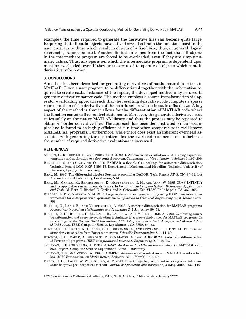
A Source Transformation via Operator Overloading Method for Generating Derivatives in MATLAB A:41
example), the time required to generate the derivative files can become quite large.Requiring that all cada objects have a fixed size also limits the functions used in theuser program to those which result in objects of a fixed size, thus, in general, logicalreferencing cannot be used. Another limitation comes from the fact that all objectsin the intermediate program are forced to be overloaded, even if they are simply nu-meric values. Thus, any operation which the intermediate program is dependent uponmust be overloaded, even if they are never used to operate on objects which containderivative information.
8. CONCLUSIONS
A method has been described for generating derivatives of mathematical functions inMATLAB. Given a user program to be differentiated together with the information re-quired to create cada instances of the inputs, the developed method may be used togenerate derivative source code. The method employs a source transformation via op-erator overloading approach such that the resulting derivative code computes a sparserepresentation of the derivative of the user function whose input is a fixed size. A keyaspect of the method is that it allows for the differentiation of MATLAB code wherethe function contains flow control statements. Moreover, the generated derivative coderelies solely on the native MATLAB library and thus the process may be repeated toobtain nth-order derivative files. The approach has been demonstrated on four exam-ples and is found to be highly efficient at run-time when compared with well knownMATLAB AD programs. Furthermore, while there does exist an inherent overhead as-sociated with generating the derivative files, the overhead becomes less of a factor asthe number of required derivative evaluations is increased.
REFERENCES
AUBERT, P., DI CÉSARÉ, N., AND PIRONNEAU, O. 2001. Automatic differentiation in C++ using expressiontemplates and application to a flow control problem. Computing and Visualization in Science 3, 197–208.
BENDTSEN, C. AND STAUNING, O. 1996. FADBAD, a flexible C++ package for automatic differentiation.Technical Report IMM–REP–1996–17, Department of Mathematical Modelling, Technical University ofDenmark, Lyngby, Denmark. aug.
BERZ, M. 1987. The differential algebra Fortran precompiler DAFOR. Tech. Report AT–3: TN–87–32, LosAlamos National Laboratory, Los Alamos, N.M.
BERZ, M., MAKINO, K., SHAMSEDDINE, K., HOFFSTÄTTER, G. H., AND WAN, W. 1996. COSY INFINITYand its applications in nonlinear dynamics. In Computational Differentiation: Techniques, Applications,and Tools, M. Berz, C. Bischof, G. Corliss, and A. Griewank, Eds. SIAM, Philadelphia, PA, 363–365.
BIEGLER, L. T. AND ZAVALA, V. M. 2008. Large-scale nonlinear programming using IPOPT: An integratingframework for enterprise-wide optimization. Computers and Chemical Engineering 33, 3 (March), 575–582.
BISCHOF, C., LANG, B., AND VEHRESCHILD, A. 2003. Automatic differentiation for MATLAB programs.Proceedings in Applied Mathematics and Mechanics 2, 1 Joh Wiley, 50–53.
BISCHOF, C. H., BÜCKER, H. M., LANG, B., RASCH, A., AND VEHRESCHILD, A. 2002. Combining sourcetransformation and operator overloading techniques to compute derivatives for MATLAB programs. InProceedings of the Second IEEE International Workshop on Source Code Analysis and Manipulation(SCAM 2002). IEEE Computer Society, Los Alamitos, CA, USA, 65–72.
BISCHOF, C. H., CARLE, A., CORLISS, G. F., GRIEWANK, A., AND HOVLAND, P. D. 1992. ADIFOR: Gener-ating derivative codes from Fortran programs. Scientific Programming 1, 1, 11–29.
BISCHOF, C. H., CARLE, A., KHADEMI, P., AND MAUER, A. 1996. ADIFOR 2.0: Automatic differentiationof Fortran 77 programs. IEEE Computational Science & Engineering 3, 3, 18–32.
COLEMAN, T. F. AND VERMA, A. 1998a. ADMAT: An Automatic Differentiation Toolbox for MATLAB. Tech-nical Report. Computer Science Department, Cornell University.
COLEMAN, T. F. AND VERMA, A. 1998b. ADMIT-1: Automatic differentiation and MATLAB interface tool-box. ACM Transactions on Mathematical Software 26, 1 (March), 150–175.
DARBY, C. L., HAGER, W. W., AND RAO, A. V. 2011. Direct trajectory optimization using a variable low-order adaptive pseudospectral method. Journal of Spacecraft and Rockets 48, 3 (May–June), 433–445.
ACM Transactions on Mathematical Software, Vol. V, No. N, Article A, Publication date: January YYYY.

A:42 M. J. Weinstein, and A. V. Rao
DOBMANN, M., LIEPELT, M., AND SCHITTKOWSKI, K. 1995. Algorithm 746: Pcomp—a fortran code forautomatic differentiation. ACM Transactions on Mathematical Software 21, 3, 233–266.
FORTH, S. A. 2006. An efficient overloaded implementation of forward mode automatic differentiation inMATLAB. ACM Transactions on Mathematical Software 32, 2 (April–June), 195–222.
GARG, D., HAGER, W. W., AND RAO, A. V. 2011. Pseudospectral methods for solving infinite-horizon optimalcontrol problems. Automatica 47, 4 (April), 829–837.
GARG, D., PATTERSON, M. A., DARBY, C. L., FRANÇOLIN, C., HUNTINGTON, G. T., HAGER, W. W., ANDRAO, A. V. 2011. Direct trajectory optimization and costate estimation of finite-horizon and infinite-horizon optimal control problems via a radau pseudospectral method. Computational Optimization andApplications 49, 2 (June), 335–358.
GARG, D., PATTERSON, M. A., HAGER, W. W., RAO, A. V., BENSON, D. A., AND HUNTINGTON, G. T. 2010. Aunified framework for the numerical solution of optimal control problems using pseudospectral methods.Automatica 46, 11 (November), 1843–1851.
GIERING, R. AND KAMINSKI, T. 1996. Recipes for adjoint code construction. Tech. Rep. 212, Max-Planck-Institut für Meteorologie.
GRIEWANK, A. 2008. Evaluating Derivatives: Principles and Techniques of Algorithmic Differentiation.Frontiers in Appl. Mathematics. SIAM Press, Philadelphia, Pennsylvania.
GRIEWANK, A., JUEDES, D., AND UTKE, J. 1996. Algorithm 755: ADOL-C, a package for the automaticdifferentiation of algorithms written in c/c++. ACM Transactions on Mathematical Software 22, 2 (April–June), 131–167.
HASCOËT, L. AND PASCUAL, V. 2004. TAPENADE 2.1 user’s guide. Rapport Technique 300, INRIA, SophiaAntipolis.
HORWEDEL, J. E. 1991. GRESS, a preprocessor for sensitivity studies of Fortran programs. In AutomaticDifferentiation of Algorithms: Theory, Implementation, and Application, A. Griewank and G. F. Corliss,Eds. SIAM, Philadelphia, PA, 243–250.
KHARCHE, R. V. 2012. Matlab automatic differentiation using source transformation.KHARCHE, R. V. AND FORTH, S. A. 2006. Source transformation for MATLAB automatic differentiation. In
Computational Science – ICCS, Lecture Notes in Computer Science, V. N. Alexandrov, G. D. van Albada,P. M. A. Sloot, and J. Dongarra, Eds. Vol. 3994. Springer, Heidelberg, Germany, 558–565.
KUBOTA, K. 1991. PADRE2, a Fortran precompiler yielding error estimates and second derivatives. InAutomatic Differentiation of Algorithms: Theory, Implementation, and Application, A. Griewank andG. F. Corliss, Eds. SIAM, Philadelphia, PA, 251–262.
MATHWORKS. 2010. Version R2010b. The MathWorks Inc., Natick, Massachusetts.MICHELOTTI, L. 1991. MXYZPTLK: A C++ hacker’s implementation of automatic differentiation. In Auto-
matic Differentiation of Algorithms: Theory, Implementation, and Application, A. Griewank and G. F.Corliss, Eds. SIAM, Philadelphia, PA, 218–227.
NOAA. 1976. U. S. standard atmosphere, 1976. National Oceanic and Amospheric [sic] Administration : forsale by the Supt. of Docs., U.S. Govt. Print. Off.
PATTERSON, M. A. AND RAO, A. V. 2012. Exploiting sparsity in direct collocation pseudospectral methodsfor solving continuous-time optimal control problems. Journal of Spacecraft and Rockets, 49, 2 (March–April), 364–377.
PATTERSON, M. A., WEINSTEIN, M. J., AND RAO, A. V. 2013. An efficient overloaded method for computingderivatives of mathematical functions in matlab. ACM Transactions on Mathematical Software, 39, 3(July), 17:1–17:36.
PRYCE, J. D. AND REID, J. K. 1998. ADO1, a Fortran 90 code for automatic differentiation. Tech. Rep. RAL-TR-1998-057, Rutherford Appleton Laboratory, Chilton, Didcot, Oxfordshire, OX11 OQX, England.
RHODIN, A. 1997. {IMAS} integrated modeling and analysis system for the solution of optimal control prob-lems. Computer Physics Communications 107, 1?3, 21 – 38.
ROSTAING-SCHMIDT, N. 1993. Différentiation automatique: Application à un problème d’optimisation enmétéorologie. Ph.D. thesis, Université de Nice-Sophia Antipolis.
RUMP, S. M. 1999. Intlab – interval laboratory. In Developments in Reliable Computing, T. Csendes, Ed.Kluwer Academic Publishers, Dordrecht, Germany, 77–104.
SHIRIAEV, D. AND GRIEWANK, A. 1996. Adol-f automatic differentiation of fortran codes. In ComputationalDifferentiation: Techniques, Applications, and Tools. SIAM, 375–384.
SPEELPENNING, B. 1980. Compiling fast partial derivatives of functions given by algorithms. Ph.D. thesis,University of Illinois at Urbana-Champaign.
TADJOUDDINE, M., FORTH, S. A., AND PRYCE, J. D. 2003. Hierarchical automatic differentiation by vertexelimination and source transformation. In Computational Science and Its Applications – ICCSA 2003,
ACM Transactions on Mathematical Software, Vol. V, No. N, Article A, Publication date: January YYYY.

A Source Transformation via Operator Overloading Method for Generating Derivatives in MATLAB A:43
Proceedings of the International Conference on Computational Science and its Applications, Montreal,Canada, May 18–21, 2003. Part II, V. Kumar, M. L. Gavrilova, C. J. K. Tan, and P. L’Ecuyer, Eds. LectureNotes in Computer Science, vol. 2668. Springer, 115–124.
WAECHTER, A. AND BIEGLER, L. T. 2006. On the implementation of a primal-dual interior-point filter linesearch algorithm for large-scale nonlinear programming. Mathematical Programming 106, 1 (March),575–582.
ACM Transactions on Mathematical Software, Vol. V, No. N, Article A, Publication date: January YYYY.