arX

iv:1

604.

0142

4v3

[as

tro-

ph.C

O]

9 J

un 2

016

A 2.4% Determination of the Local Value of the Hubble Constant1

Adam G. Riess2,3, Lucas M. Macri4, Samantha L. Hoffmann4, Dan Scolnic2,5, Stefano Casertano3,

Alexei V. Filippenko6, Brad E. Tucker6,7, Mark J. Reid8, David O. Jones2, Jeffrey M. Silverman9,

Ryan Chornock10, Peter Challis8, Wenlong Yuan4, Peter J. Brown4, and Ryan J. Foley11,12

ABSTRACT

We use the Wide Field Camera 3 (WFC3) on the Hubble Space Telescope (HST) to

reduce the uncertainty in the local value of the Hubble constant from 3.3% to 2.4%.

The bulk of this improvement comes from new, near-infrared observations of Cepheid

variables in 11 host galaxies of recent type Ia supernovae (SNe Ia), more than doubling

the sample of reliable SNe Ia having a Cepheid-calibrated distance to a total of 19; these

in turn leverage the magnitude-redshift relation based on ∼ 300 SNe Ia at z<0.15. All

19 hosts as well as the megamaser system NGC4258 have been observed with WFC3

in the optical and near-infrared, thus nullifying cross-instrument zeropoint errors in the

relative distance estimates from Cepheids. Other noteworthy improvements include a

33% reduction in the systematic uncertainty in the maser distance to NGC4258, a larger

sample of Cepheids in the Large Magellanic Cloud (LMC), a more robust distance to

the LMC based on late-type detached eclipsing binaries (DEBs), HST observations of

Cepheids in M31, and new HST-based trigonometric parallaxes for Milky Way (MW)

Cepheids.

1Based on observations with the NASA/ESA Hubble Space Telescope, obtained at the Space Telescope Science

Institute, which is operated by AURA, Inc., under NASA contract NAS 5-26555.

2Department of Physics and Astronomy, Johns Hopkins University, Baltimore, MD, USA

3Space Telescope Science Institute, Baltimore, MD, USA; ariess@stsci.edu

4George P. and Cynthia Woods Mitchell Institute for Fundamental Physics and Astronomy, Department of Physics

& Astronomy, Texas A&M University, College Station, TX, USA

5Kavli Institute for Cosmological Physics, University of Chicago, Chicago, IL, USA

6Department of Astronomy, University of California, Berkeley, CA, USA

7The Research School of Astronomy and Astrophysics, Australian National University, Mount Stromlo Observa-

tory, Weston Creek, ACT, Australia

8Harvard-Smithsonian Center for Astrophysics, Cambridge, MA, USA

9Department of Astronomy, University of Texas, Austin, TX, USA

10Astrophysical Institute, Department of Physics and Astronomy, Ohio University, Athens, OH, USA

11Department of Physics, University of Illinois at Urbana-Champaign, Urbana, IL, USA

12Department of Astronomy, University of Illinois at Urbana-Champaign, Urbana, IL, USA

– 2 –

We consider four geometric distance calibrations of Cepheids: (i) megamasers in

NGC4258, (ii) 8 DEBs in the LMC, (iii) 15 MW Cepheids with parallaxes measured with

HST/FGS, HST/WFC3 spatial scanning and/or Hipparcos, and (iv) 2 DEBs in M31.

The Hubble constant from each is 72.25±2.51, 72.04±2.67, 76.18±2.37, and 74.50±3.27

km s−1 Mpc−1, respectively. Our best estimate of H0 = 73.24 ± 1.74 km s−1 Mpc−1

combines the anchors NGC4258, MW, and LMC, yielding a 2.4% determination (all

quoted uncertainties include fully-propagated statistical and systematic components).

This value is 3.4σ higher than 66.93 ± 0.62 km s−1 Mpc−1 predicted by ΛCDM with 3

neutrino flavors having a mass of 0.06 eV and the new Planck data, but the discrep-

ancy reduces to 2.1σ relative to the prediction of 69.3± 0.7 km s−1Mpc−1 based on the

comparably precise combination of WMAP+ACT+SPT+BAO observations, suggesting

that systematic uncertainties in cosmic microwave background radiation measurements

may play a role in the tension.

If we take the conflict between Planck high-redshift measurements and our local

determination of H0 at face value, one plausible explanation could involve an additional

source of dark radiation in the early Universe in the range of ∆Neff ≈ 0.4−1. We

anticipate further significant improvements in H0 from upcoming parallax measurements

of long-period MW Cepheids.

Subject headings: galaxies: distances and redshifts — cosmology: observations — cos-

mology: distance scale — supernovae: general — stars: variables: Cepheids

1. Introduction

The Hubble constant (H0) measured locally and the sound horizon observed from the cosmic

microwave background radiation (CMB) provide two absolute scales at opposite ends of the visible

expansion history of the Universe. Comparing the two gives a stringent test of the standard cosmo-

logical model. A significant disagreement would provide evidence for fundamental physics beyond

the standard model, such as time-dependent or early dark energy, gravitational physics beyond

General Relativity, additional relativistic particles, or nonzero curvature. Indeed, none of these

features has been excluded by anything more compelling than a theoretical preference for simplic-

ity over complexity. In the case of dark energy, there is no simple explanation at present, leaving

direct measurements as the only guide among numerous complex or highly tuned explanations.

Recent progress in measuring the CMB fromWMAP (Hinshaw et al. 2013; Bennett et al. 2013)

and Planck (Planck Collaboration et al. 2016) have reduced the uncertainty in the distance to the

surface of last scattering (z ∼ 1000) to below 0.5% in the context of ΛCDM, motivating complemen-

tary efforts to improve the local determination of H0 to percent-level precision (Suyu et al. 2012;

Hu 2005). Hints of mild tension at the ∼2−2.5σ level with the 3−5% measurements of H0 stated by

Riess et al. (2011), Sorce et al. (2012), Freedman et al. (2012), and Suyu et al. (2013) have been

– 3 –

widely considered and in some cases revisited in great detail (Efstathiou 2014; Dvorkin et al. 2014;

Bennett et al. 2014; Spergel et al. 2015; Becker et al. 2015), with no definitive conclusion except

for highlighting the value of improvements in the local observational determination of H0.

1.1. Past Endeavors

Considerable progress in the local determination of H0 has been made in the last 25 years, as-

sisted by observations of water masers, strong-lensing systems, SNe, the Cepheid period-luminosity

(P–L) relation (also known as the Leavitt law; Leavitt & Pickering 1912), and other sources

used independently or in concert to construct distance ladders (see Freedman & Madore 2010;

Livio & Riess 2013, for recent reviews).

A leading approach utilizes Hubble Space Telescope (HST) observations of Cepheids in the hosts

of recent, nearby SNe Ia to link geometric distance measurements to other SNe Ia in the expanding

Universe. The SN Ia HST Calibration Program (Sandage et al. 2006) and the HST Key Project

(Freedman et al. 2001) both made use of HST observations with WFPC2 to resolve Cepheids in

SN Ia hosts. However, the useful range of that camera for measuring Cepheids, .25 Mpc, placed

severe limits on the number and choice of SNe Ia which could be used to calibrate their luminosity

(e.g., SNe 1937C, 1960F, 1974G). A dominant systematic uncertainty resulted from the unreliability

of those nearby SNe Ia which were photographically observed, highly reddened, spectroscopically

abnormal, or discovered after peak brightness. Only two objects (SNe 1990N and 1981B) used

by Freedman et al. (2001, 2012) and four by Sandage et al. (2006) (the above plus SN 1994ae

and SN1998aq) were free from these shortcomings, leaving a very small set of reliable calibrators

relative to the many hundreds of similarly reliable SNe Ia observed in the Hubble flow. The resulting

ladders were further limited by the need to calibrate WFPC2 at low flux levels to the ground-based

systems used to measure Cepheids in a single anchor, the Large Magellanic Cloud (LMC). The

use of LMC Cepheids introduces additional systematic uncertainties because of their shorter mean

period (∆〈log P 〉 ≈ 0.7 dex) and lower metallicity (∆ log(O/H) = −0.25 dex, Romaniello et al.

2008) than those found with HST in the large spiral galaxies that host nearby SNe Ia. Despite

careful work, the estimates of H0 by the two teams (each with 10% uncertainty) differed by 20%,

owing in part to the aforementioned systematic errors.

More recently, the SH0ES (Supernovae, H0, for the Equation of State of dark energy) team

used a number of advancements to refine this approach to determining H0. Upgrades to the in-

strumentation of HST doubled its useful range for resolving Cepheids (leading to an eight-fold

improvement in volume and in the expected number of useful SN Ia hosts), first with the Ad-

vanced Camera for Surveys (ACS; Riess et al. 2005, 2009b) and later with the Wide Field Camera

3 (WFC3; Riess et al. 2011, hereafter R11) owing to the greater area, higher sensitivity, and smaller

pixels of these cameras. WFC3 has other superior features for Cepheid reconnaissance, including a

white-light filter (F350LP) that more than doubles the speed for discovering Cepheids and measur-

ing their periods relative to the traditional F555W filter, and a 5 square arcmin near-infrared (NIR)

– 4 –

detector that can be used to reduce the impact of differential extinction and metallicity differences

across the Cepheid sample. A precise geometric distance to NGC4258 measured to 3% using water

masers (Humphreys et al. 2013, hereafter H13) has provided a new anchor galaxy whose Cepheids

can be observed with the same instrument and filters as those in SN Ia hosts to effectively cancel

the effect of photometric zeropoint uncertainties in this step along the distance ladder. Tied to the

Hubble diagram of 240 SNe Ia (now >300 SNe Ia; Scolnic et al. 2015; Scolnic & Kessler 2016), the

new ladder was used to initially determine H0 with a total uncertainty of 4.7% (Riess et al. 2009a,

hereafter R09). R11 subsequently improved this measurement to 3.3% by increasing to 8 the num-

ber of Cepheid distances to reliable SN Ia hosts, and formally including HST/FGS trigonometric

parallaxes of 10 Milky Way (MW) Cepheids with distance D<0.5 kpc and individual precision of

8% (Benedict et al. 2007). The evolution of the error budget in these measurements is shown in

Figure 1.

Here we present a broad set of improvements to the SH0ES team distance ladder including

new near-infrared HST observations of Cepheids in 11 SN Ia hosts (bringing the total to 19), a

refined computation of the distance to NGC4258 from maser data, additional Cepheid parallax

measurements, larger Cepheid samples in the anchor galaxies, and additional SNe Ia to constrain

the Hubble flow. We present the new Cepheid data in §2 and in S. L. Hoffmann et al. (2016, in

prep.; hereafter H16). Other improvements are described throughout §3, and a consideration of

analysis variants and systematic uncertainties is given in §4. We end with a discussion in §5.

2. HST Observations of Cepheids in the SH0ES Program

Discovering and measuring Cepheid variables in SN Ia host galaxies requires a significant

investment of observing time on HST. It is thus important to select SN Ia hosts likely to produce

a set of calibrators that is a good facsimile of the much larger sample defining the modern SN Ia

magnitude-redshift relation at 0.01 < z < 0.15 (e.g., Scolnic et al. 2015; Scolnic & Kessler 2016).

Poor-quality light curves, large reddening, atypical SN explosions, or hosts unlikely to yield a

significant number of Cepheids would all limit contributions to this effort. Therefore, the SH0ES

program has been selecting SNe Ia with the following qualities to ensure a reliable calibration of

their fiducial luminosity: (1) modern photometric data (i.e., photoelectric or CCD), (2) observed

before maximum brightness and well thereafter, (3) low reddening (implying AV < 0.5 mag), (4)

spectroscopically typical, and (5) a strong likelihood of being able to detect Cepheids in its host

galaxy with HST. This last quality translates into any late-type host (with features consistent with

the morphological classification of Sa to Sd) having an expectation of D . 40 Mpc, inclination

<75, and apparent size >1′. To avoid a possible selection bias in SN Ia luminosities, the probable

distance of the host is estimated via the Tully-Fisher relation or flow-corrected redshifts as reported

– 5 –

in NED1. We will consider the impact of these selections in §4.

The occurrence of SNe Ia with these characteristics is unfortunately quite rare, leading to a

nearly complete sample of 19 objects observed between 1993 and 2015 (see Table 1). Excluding

supernovae from the 1980s, a period when modern detectors were rare and when suitable SNe Ia

may have appeared and gone unnoticed, the average rate of production is ∼ 1/year. Regrettably, it

will be difficult to increase this sample substantially (by a factor of ∼ 2) over the remaining lifetime

of HST. We estimate that a modest augmentation of the sample (at best) would occur by removing

one or more of the above selection criteria, but the consequent increase in systematic uncertainty

would more than offset the statistical gain.

Reliable SNe Ia from early-type hosts could augment the sample, with distance estimates based

on RR Lyrae stars or the tip of the red-giant branch (TRGB) for their calibration. Unfortunately,

the reduced distance range of these distance indicators for HST compared to Cepheids (2.5 mag or

D< 13 Mpc for TRGB, 5 mag or D< 4 Mpc for RR Lyrae stars) and the factor of ∼ 5 smaller

sample of SNe Ia in early-type hosts limits the sample increase to just a few additional objects

(SN 1994D, SN 1980N, 1981D, and SN 2006dd with the latter 3 all in the same host; Beaton et al.

2016), a modest fraction of the current sample of 19 SNe Ia calibrated by Cepheids.

Figure 2 shows the sources of the HST data obtained on every host we use, gathered from

different cameras, filters, time periods, HST programs and observers. All of these publicly available

data can be readily obtained from the Mikulski Archive for Space Telescopes (MAST; see Table 1).

The utility of the imaging data can be divided into two basic functions: Cepheid discovery and flux

measurement. For the former, a campaign using a filter with central wavelength in the visual band

and ∼12 epochs with nonredundant spacings spanning ∼60–90 days will suffice to identify Cepheid

variables by their unique light curves and accurately measure their periods (Madore & Freedman

1991; Saha et al. 1996; Stetson 1996). Revisits on a year timescale, although not required, will

yield increased phasing accuracy for the longest-period Cepheids. Image subtraction can be very

effective for finding larger samples of variables (Bonanos & Stanek 2003), but the additional objects

will be subject to greater photometric biases owing to blends which suppress their amplitudes and

chances of discovery in time-series data (Ferrarese et al. 2000).

Flux measurements are required in order to use Cepheids as standard candles for distance

measurement and are commonly done with HST filters at known phases in optical (F555W, F814W)

and NIR (F160W) bands to correct for the effects of interstellar dust and the nonzero width in

temperature of the Cepheid instability strip. We rely primarily on NIR “Wesenheit” magnitudes

(Madore 1982), defined as

mWH = mH −R (V −I), (1)

where H = F160W , V = F555W , I = F814W in the HST system, and R ≡ AH/(AV −AI). We

1The NASA/IPAC Extragalactic Database (NED) is operated by the Jet Propulsion Laboratory, California Insti-

tute of Technology, under contract with the National Aeronautics and Space Administration (NASA).

– 6 –

note that the value of R due to the correlation between Cepheid intrinsic color and luminosity is

very similar to that due to extinction (Macri et al. 2015), so the value of R derived for the latter

effectively also reduces the intrinsic scatter caused by the breadth of the instability strip. However,

to avoid a distance bias, we include only Cepheids with periods above the completeness limit of

detection (given in H16) in our primary fit. (In future work we will use simulations to account for

the bias of Cepheids below this limit to provide an extension of the Cepheid sample.)

In HST observations, Cepheid distances based on NIR measurements have somewhat higher

statistical uncertainties than those solely based on optical photometry owing to the smaller field of

view, lower spatial resolution, and greater blending from red giants. However, as characterized in

§4.2, this is more than offset by increased robustness to systematic uncertainties (such as metallicity

effects and possible breaks in the slope of the P–L relation) as well as the reduced impact of

extinction and a lower sensitivity to uncertainties in the reddening law. The latter is quantified

by the value of R in Equation 1, ranging from 0.3 to 0.5 at H depending on the reddening law,

a factor of ∼ 4 lower than the value at I. At the high end, the Cardelli et al. (1989) formulation

with RV = 3.3 yields R = 0.47. The Fitzpatrick (1999) formulation with RV = 3.3 and 2.5 yields

R = 0.39 and R = 0.35, respectively. At the low end, a formulation appropriate for the inner Milky

Way (Nataf et al. 2016) yields R = 0.31. We analyze the sensitivity of H0 to variations in R in §4.

2.1. Cepheid Photometry

The procedure for identifying Cepheids from time-series optical data (see Table 1 and Figure 2)

has been described extensively (Saha et al. 1996; Stetson 1996; Riess et al. 2005; Macri et al. 2006);

details of the procedures followed for this sample are presented by H16, utilize the DAO suite of

software tools for crowded-field PSF photometry, and are similar to those used previously by the

SH0ES team. The complete sample of Cepheids discovered or reanalyzed by H16 in these galaxies

(NGC4258 and the 19 SN Ia hosts) at optical wavelengths contains 2113 variables above the periods

for completeness across the instability strip (with limits estimated using the HST exposure-time

calculators and empirical tests as described in that publication). There are 1566 such Cepheids in

the 19 SN Ia hosts within the smaller WFC3-IR fields alone. The positions of the Cepheids within

each target galaxy are shown in Figure 3. For hosts in which we used F350LP to identify Cepheid

light curves, additional photometry was obtained over a few epochs in F555W and F814W. These

data were phase-corrected to mean-light values using empirical relations based on light curves

in both F555W and F350LP from Cepheids in NGC5584. Figure 4 shows composite Cepheid

light curves in F350LP/F555W for each galaxy. Despite limited sampling of the individual light

curves, the composites clearly display the characteristic “saw-toothed” light curves of Population I

fundamental-mode Cepheids, with a rise twice as fast as the decline and similar mean amplitudes

across all hosts.

For every host, optical data in F555W and F814W from WFC3 were uniformly calibrated

using the latest reference files from STScI and aperture corrections derived from isolated stars in

– 7 –

Table 1. Cepheid Hosts Observed with HST/WFC3

Galaxy SN Ia Exp. time (s) Prop IDs UT Datec

NIRa Opt.b

M101d 2011fe 4847 3776 12880 2013-03-03

N1015 2009ig 14364 39336 12880 2013-06-30

N1309d 2002fk 6991 3002 11570,12880 2010-07-24

N1365d 2012fr 3618 3180 12880 2013-08-06

N1448 2001el 6035 17562 12880 2013-09-15

N2442 2015F 6035 20976 13646 2016-01-21

N3021d 1995al 4426 2962 11570,12880 2010-06-03

N3370d 1994ae 4376 2982 11570,12880 2010-04-04

N3447 2012ht 4529 19114 12880 2013-12-15

N3972 2011by 6635 19932 13647 2015-04-19

N3982d 1998aq 4018 1400 11570 2009-08-04

N4038d 2007sr 6795 2064 11577 2010-01-22

N4258d Anchor 34199 6120 11570 2009-12-03

N4424 2012cg 3623 17782 12880 2014-01-08

N4536d 1981B 2565 2600 11570 2010-07-19

N4639d 1990N 5379 1600 11570 2009-08-07

N5584 2007af 4929 59940 11570 2010-04-04

N5917 2005cf 7235 23469 12880 2013-05-20

N7250 2013dy 5435 18158 12880 2013-10-12

U9391 2003du 13711 39336 12880 2012-12-14

Note. — (a) Data obtained with WFC3/IR and F160W. (b) Data

obtained with WFC3/UVIS and F555W, F814W, or F350LP used

to find and measure the flux of Cepheids. (c) Date of first WFC3/IR

observation. (d) Includes time-series data from an earlier program

and a different camera — see Fig. 2.

– 8 –

deep images to provide uniform flux measurements for all Cepheids. In a few cases, F555W and

F814W data from ACS and WFC3 were used in concert with their well-defined cross-calibration to

obtain photometry with a higher signal-to-noise ratio (S/N). The cross-calibration between these

two cameras has been stable to <0.01 mag over their respective lifetimes.

As in R11, we calculated the positions of Cepheids in the WFC3 F160W images using a

geometric transformation derived from the optical images using bright and isolated stars, with

resulting mean position uncertainties for the variables <0.03 pix. We used the same scene-modeling

approach to F160W NIR photometry developed in R09 and R11. The procedure is to build a model

of the Cepheid and sources in its vicinity using the superposition of point-spread functions (PSFs).

The position of the Cepheid is fixed at its predicted location to avoid measurement bias. We model

and subtract a single PSF at that location and then produce a list of all unresolved sources within

50 pixels. A scene model is constructed with three parameters per source (x, y, and flux), one

for the Cepheid (flux) and a local sky level in the absence of blending; the best-fit parameters

are determined simultaneously using a Levenberg-Marquardt-based algorithm. Example NIR scene

models for each of the 19 SN Ia hosts are shown in Figure 5.

Care must be taken when measuring photometry of visible stellar sources in crowded regions

as source blending can alter the statistics of the Cepheid background (Stetson 1987). Typically the

mean flux of pixels in an annulus around the Cepheid is subtracted from the measured flux at the

position of the Cepheid to produce unbiased photometry of the Cepheid. This mean background

or sky would include unresolved sources and diffuse background. However, we can improve the

precision of Cepheid photometry by correctly attributing some flux to the other sources in the

scene, especially those visibly overlapping with the Cepheid. The consequence of differentiating the

mean sky into individual source contributions plus a lower constant sky level is that the new sky

level will underestimate the true mix of unresolved sources and diffuse background superimposed

with the Cepheid flux (in sparse regions without blending, the original and new sky levels would

approach the same value). This effect may usefully be called the sky bias or the photometric

difference due to blending and is statistically easily rectified. To retrieve the unbiased Cepheid

photometry from the result of the scene model we could either recalculate the Cepheid photometry

using the original mean sky or correct the overestimate of Cepheid flux based on the measured

photometry of artificial stars added to the scenes. The advantage of the artificial star approach is

that the same analysis also produces an empirical error estimate and can provide an estimate of

outlier frequency.

Following this approach, we measure the mean difference between input and recovered pho-

tometry of artificial Cepheids added to the local scenes in the F160W images and fit with the same

algorithms. As in R09 and R11, we added and fitted 100 artificial stars, placed one at a time, at

random positions within 5 arcseconds of (but not coincident with) each Cepheid to measure and

account for this difference. To avoid a bias in this procedure, we initially estimate the input flux for

the artificial stars from the Cepheid period and an assumed P–L relation (iteratively determined),

measure the difference caused by blending, refine the P–L relation, and iterate until convergence.

– 9 –

Additionally, we use the offset in the predicted and measured location of the Cepheid, a visible

consequence of blending, to select similarly affected artificial stars to customize the difference mea-

surements for each Cepheid. The median difference for the Cepheids in all SN hosts hosts observed

with HST is 0.18 mag, mostly due to red-giant blends, and it approaches zero for Cepheids in

lower-density regions such as the outskirts of hosts. The Cepheid photometry presented in this

paper already accounts for the sky bias. We also estimate the uncertainty in the Cepheid flux from

the dispersion of the measured artificial-star photometry around the 2.7σ-clipped mean. The NIR

Cepheid P–L relations for all hosts and anchors are shown in Figure 6.

Likewise, in the optical images, we used as many as 200 measurements of randomly placed

stars in the vicinity of each Cepheid in F555W and F814W images to measure and account for the

photometric difference due to the process of estimating the sky in the presence of blending. Only

10 stars at a time were added to each simulated image to avoid increasing the stellar density. These

tests show that similarly to the NIR measurements, uncertainty in the Cepheid background is the

leading source of scatter in the observed P–L relations of the SN hosts. The mean dispersions

at F555W and F814W, with values for each host listed in Table 2 in columns 6 and 7, are 0.19

and 0.17 mag, respectively. All SN hosts and NGC4258 display some difference in their optical

magnitudes due to blending, with mean values of 0.05 and 0.06 mag (bright) in F555W and F814W,

respectively. The most crowded case (∆V = 0.32 and ∆I = 0.26 mag) is NGC4424, a galaxy whose

Cepheids are located in a circumnuclear starburst region with prominent dust lanes. We tabulate

the mean photometric differences due to blending for each host in Table 2, columns 2 and 3.

However, the effect of blending largely cancels when determining the color F555W−F814W used

to measure Cepheid distances via equation (1) since the blending is highly correlated across these

bands. Indeed, the estimated change in color across all hosts given in Table 2, column 4 has

a mean of only 0.005 mag (blue) and a host-to-host scatter of 0.01 mag, implying no statistically

significant difference from the initial measurement and thus we have not applied these to the optical

magnitudes in Table 4. Even the additional scatter in the mWH P–L relation owing to blending in

the optical color measurement is a relatively minor contribution of 0.07 mag. The small correction

due to blending in the optical bands does need to be accounted for when using a conventional

optical Wesenheit magnitude, mWI =F814W−RI(F555W−F814W), because (unlike the color) the

cancellation in mWI is not complete. We find a small mean difference for mW

I in our SN hosts

of 0.025 mag (bright) with a host-to-host dispersion in this quantity of 0.03 mag. If uncorrected,

this would lead to a 1% underestimate of distances and an overestimate of H0 for studies that rely

exclusively on mWI . The more symmetric effect of blending on mW

I than mWH magnitudes results

from the mixture of blue blends (which make mWI faint) and red blends (which make mW

I bright).

These results are consistent with those found from simulations by Ferrarese et al. (2000), who drew

similar conclusions. We will make use of these results for mWI in §4.2. Although the net effect of

blending for mWI is typically small, the uncertainty it produces is the dominant source of dispersion

with a mean of 0.36 mag for the SN hosts, similar in impact and scatter to what was found for

mWH .

– 10 –

Table 2. Artificial Cepheid Tests in Optical Images

Host ∆V ∆I ∆ct ∆mWI σ(V ) σ(I) σct σ(mW

I )

[mmag] [mag]

M101 6 3 1 -2 0.09 0.09 0.03 0.16

N1015 41 40 1 27 0.13 0.13 0.06 0.31

N1309 105 63 12 -1 0.35 0.26 0.10 0.48

N1365 15 19 0 7 0.13 0.13 0.06 0.29

N1448 31 24 1 6 0.14 0.13 0.06 0.29

N2442 141 109 8 23 0.24 0.21 0.10 0.48

N3021 106 134 0 75 0.23 0.22 0.09 0.46

N3370 69 55 5 26 0.23 0.19 0.07 0.37

N3447 34 23 4 -1 0.14 0.12 0.06 0.29

N3972 79 68 7 25 0.18 0.17 0.07 0.38

N3982 82 69 0 22 0.22 0.19 0.09 0.44

N4038 38 28 2 12 0.19 0.15 0.07 0.34

N4258I 5 7 -1 10 0.20 0.23 0.05 0.36

N4258O -2 1 0 0 0.08 0.07 0.02 0.10

N4424 318 262 -2 111 0.31 0.28 0.11 0.58

N4536 12 16 -1 10 0.11 0.10 0.05 0.24

N4639 56 85 -5 89 0.21 0.22 0.09 0.51

N5584 26 23 2 7 0.15 0.13 0.05 0.26

N5917 54 51 -2 32 0.20 0.19 0.08 0.42

N7250 152 91 13 -1 0.24 0.20 0.08 0.42

U9391 36 42 -3 38 0.15 0.15 0.06 0.34

Note. — ∆ = median magnitude or color offset derived from tests;

σ =dispersion around ∆; V stands for F555W; I stands for F814W;

ct= R× (V −I), with R = 0.39 for RV = 3.3 and the Fitzpatrick (1999)

extinction law; mWI =defined in text.

– 11 –

Table 3. Properties of NIR P–L Relations

Galaxy Number 〈P 〉 ∆T 〈σtot〉 σPL

FoV meas. fit (days) (days)

LMC . . . 799 785 6.6 . . . 0.09 0.08

MW . . . 15 15 8.5 . . . 0.21 0.12

M31 . . . 375 372 11.5 0 0.15 0.15

M101 355 272 251 17.0 0 0.30 0.32

N1015 27 14 14 59.8 100 0.32 0.36

N1309 64 45 44 55.2 0 0.35 0.36

N1365 73 38 32 33.6 12 0.32 0.32

N1448 85 60 54 30.9 54 0.30 0.36

N2442 285 143 141 32.5 68 0.52 0.38

N3021 36 18 18 32.8 0 0.42 0.51

N3370 86 65 63 42.1 0 0.33 0.33

N3447 120 86 80 34.5 59 0.28 0.34

N3972 71 43 42 31.5 38 0.49 0.38

N3982 22 16 16 40.6 0 0.30 0.32

N4038 28 13 13 63.4 0 0.43 0.33

N4258 228 141 139 18.8 0 0.40 0.36

N4424 8 4 3 28.9 33 0.56 . . .

N4536 47 35 33 36.5 0 0.27 0.29

N4639 35 26 25 40.4 0 0.36 0.45

N5584 128 85 83 42.6 11 0.32 0.33

N5917 21 14 13 39.8 100 0.39 0.38

N7250 39 22 22 31.3 60 0.44 0.43

U9391 36 29 28 42.2 100 0.34 0.43

Total SN 1566 1028 975 32.5 . . . . . . . . .

Total All . . . 2358 2286 . . . . . . . . . . . .

Note. — FoV: located within the WFC3/IR field of view. Meas.: good

quality measurement within allowed color range and with period above

completeness limit. Fit: after global outlier rejection, see §4.1. 〈P 〉: me-

dian period of the final NIR sample used in this analysis; ∆T =time

interval between first and last NIR epochs; 〈σtot〉 =median value of

σtot (uncertainties) for Cepheids in each host (see text for definition);

σPL =apparent dispersion of NIR P–L relation after outlier rejection.

– 12 –

Although we quantify and propagate the individual measurement uncertainty for each Cepheid,

we conservatively discard the lowest-quality measurements. As in R11, scene models of Cepheids

were considered to be useful if our software reported a fitted magnitude for the source with an

uncertainty < 0.7 mag, a set of model residual pixels with root-mean square (rms) lower than

3σ from the other Cepheid scenes, and a measured difference from the artificial star analyses of

<1.5 mag. In addition, we used a broad (1.2 mag) allowed range of F814W−F160W colors centered

around the median for each host, similar to the V−I color selection common to optical studies (see

H16), to remove any Cepheids strongly blended with redder or bluer stars of comparable brightness.

As simulations in §4.1 show, most of these result from red giants but also occasionally from blue

supergiants.

1028 of the 1566 Cepheids present in the F160W images of the SN Ia hosts with periods above

their respective completeness limits yielded a good quality photometric measurement within the

allowed color range. Excessive blending in the vicinity of a Cepheid in lower-resolution and lower-

contrast NIR images was the leading cause for the failure to derive a useful measurement for the

others. The number of Cepheids available at each step in the measurement process is given in

Table 3.

2.2. Statistical Uncertainties in Cepheid Distances

We now quantify the statistical uncertainties that apply to Cepheid-based distance estimates.

As described in the previous section, the largest source of measurement uncertainty for mWH (defined

in equation 1) arises from fluctuations in the NIR sky background due to variations in blending,

and it is measured from artificial star tests; we refer to this as σsky. For SN Ia hosts at 20–40 Mpc

and for NGC4258, the mean σsky for Cepheids in the NIR images is 0.28 mag, but it may be higher

or lower depending on the local stellar density. The next term which may contribute uncertainty

in equation 1 is σct = Rσ(V − I). While blending does not change the mean measured optical

colors (discussed in §2.1), it does add a small amount of dispersion. The artificial star tests in

the optical data yield a mean value for σct of 0.07 mag across all hosts, with values for each host

given in Table 2, column 8). There is also an intrinsic dispersion, σint, resulting from the nonzero

temperature width of the Cepheid instability strip. It can be determined empirically using nearby

Cepheid samples which have negligible background errors. We find σint = 0.08 mag for mWH (0.12

mag for mWI ) using the LMC Cepheids from Macri et al. (2015) over a comparable period range

(see Figure 6). This agrees well with expectations from the Geneva stellar models (R. I. Anderson

et al. 2016, in prep.). We use this value as the intrinsic dispersion of mean mWH magnitudes.

The last contribution comes from our use of random- or limited-phase (rather than mean-phase)

F160W magnitudes. Monte Carlo sampling of complete H-band light curves from Persson et al.

– 13 –

(2004) shows that the use of a single random phase adds an error of σph =0.12 mag2. The relevant

fractional contribution of the random-phase uncertainty for a given Cepheid with period P depends

on the temporal interval, ∆T , across NIR epochs, a fraction we approximate as fph = 1− (∆T/P )

for ∆T < P and fph = 1 for ∆T > P ; the values of ∆T are given in Table 3. The value of this

fraction ranges from ∼1 (NIR observations at every optical epoch) to zero (a single NIR follow-up

observation).

Thus, we assign a total statistical uncertainty arising from the quadrature sum of four terms:

NIR photometric error, color error, intrinsic width and random-phase:

σtot = (σ2sky+σ2

ct+σ2int+(fphσph)

2)12 .

We give the values of σtot for each Cepheid in Table 4. These have a median of 0.30 mag (mean of

0.32 mag) across all fields; mean values for each field range from 0.23 mag (NGC3447) to 0.47 mag

(NGC4424). The mean for NGC4258 is 0.39 mag. We also include in Table 4 an estimate of the

metallicity at the position of each Cepheid based on metallicity gradients measured from optical

spectra of H II regions obtained with the Keck-I 10 m telescope and presented by H16.

3. Measuring the Hubble Constant

The determination of H0 follows the formalism described in §3 of R09. To summarize, we

perform a single, simultaneous fit to all Cepheid and SN Ia data to minimize one χ2 statistic and

measure the parameters of the distance ladder. We use the conventional definition of the distance

modulus, µ = 5 logD+25, with D a luminosity distance in Mpc and measured as the difference in

magnitudes of an apparent and absolute flux, µ = m−M . We express the jth Cepheid magnitude

in the ith host as

mWH,i,j = (µ0,i−µ0,N4258)+zpW,N4258+bW log Pi,j+ZW ∆ log (O/H)i,j , (2)

where the individual Cepheid parameters are given in Table 4 and mWH,i,j was defined in Equation 1.

We determine the values of the nuisance parameters bW and ZW — which define the relation

between Cepheid period, metallicity, and luminosity — by minimizing the χ2 for the global fit to

the sample data. The reddening-free distances for the hosts relative to NGC4258 are given by the

fit parameters µ0,i−µ0,N4258, while zpW,N4258 is the intercept of the P–L relation simultaneously fit

to the Cepheids of NGC4258.

Uncertainties in the nuisance parameters are due to measurement errors and the limited period

and metallicity range spanned by the variables. In R11 we used a prior inferred from external

2The sum of the intrinsic and random phase errors, 0.14 mag, is smaller than the 0.21 mag assumed by R11; the

overestimate of this uncertainty explains why the χ2 of the P–L fits in that paper were low and resulted in the need

to rescale parameter errors.

– 14 –

Cepheid datasets to help constrain these parameters. In the present analysis, instead, we explicitly

use external data as described below to augment the constraints.

Recent HST observations of Cepheids in M31 provide a powerful ancillary set of Cepheids at

a fixed distance to help characterize NIR P–L relations. Analyses of the HST PHAT Treasury

data (Dalcanton et al. 2012) by Riess et al. (2012), Kodric et al. (2015), and Wagner-Kaiser et al.

(2015) used samples of Cepheids discovered from the ground with NIR and optical magnitudes

from HST to derive low-dispersion P–L relations. We used the union set of these samples and their

WFC3 photometry in F160W measured with the same algorithms as the previous hosts to produce

a set of 375 Cepheids with 3 < P < 78 d as shown in Figure 6. We add Equation 2 (actually, a

set of such equations) for these data to those from the other hosts, requiring the addition of one

nuisance parameter, the distance to M31, but providing a large range of log P (∼1.4 dex) for the

determination of the P–L relation slopes. These M31 Cepheids alone constrain the slope to an

uncertainty of 0.03 mag dex−1, a factor of 3 better than the prior used by R11. They also hint at

the possible evidence of a break in the mWH P–L relation at the 2σ confidence level (Kodric et al.

2015) if the location of a putative break is assumed a priori to be at 10 days as indicated by optical

P–L relations (Ngeow & Kanbur 2005). To allow for a possible break, we include two different slope

parameters in Equation 2 in the primary analysis, one for Cepheids with P >10 d and another for

P <10 d. We will consider alternative approaches for dealing with nonlinear P–L relations in §4.1.

The SN Ia magnitudes in the calibrator sample are simultaneously expressed as

m0x,i = (µ0,i − µ0,N4258) +m0

x,N4258, (3)

where the value m0x,i is the maximum-light apparent x-band brightness of a SN Ia in the ith

host at the time of B-band peak, corrected to the fiducial color and luminosity. This quantity is

determined for each SN Ia from its multiband light curves and a light-curve fitting algorithm. For

the primary fits we use SALT-II (Guy et al. 2005; Guy et al. 2010). For consistency with the most

recent cosmological fits we use version 2.4 of SALT II as used by Betoule et al. (2014) and more

recently from Scolnic & Kessler (2016) 3 and for which x = B. The fit parameters are discussed in

more detail in §4.2. In order to compare with R11 and to explore systematics in light-curve fits,

we also use MLCS2k2 (Jha et al. 2007) for which x = V (see §4.2 for further discussion).

The simultaneous fit to all Cepheid and SN Ia data via Equations 2 and 3 results in the

determination of m0x,N4258, which is the expected reddening-free, fiducial, peak magnitude of a

SN Ia appearing in NGC4258. The individual Cepheid P–L relations are shown in Figure 6.

Lastly, H0 is determined from

log H0 =(m0

x,N4258 − µ0,N4258) + 5ax + 25

5, (4)

where µ0,4258 is the independent, geometric distance modulus estimate to NGC4258 obtained

3http://kicp.uchicago.edu/∼dscolnic/Supercal/supercal vH0.fitres

– 15 –

through VLBI observations of water megamasers orbiting its central supermassive black hole

(Herrnstein et al. 1999; Humphreys et al. 2005; Argon et al. 2007; Humphreys et al. 2008, 2013).

Observations of megamasers in Keplerian motion around a supermassive blackhole in NGC 4258

provide one of the best sources of calibration of the absolute distance scale with a total uncertainty

given by H13 of 3%. However, the leading systematic error in H13 resulted from limited numerical

sampling of the multi-parameter model space of the system, given in H13 as 1.5%. The ongoing

improvement in computation speed allows us to reduce this error.

Here we make use of an improved distance estimate to NGC4258 utilizing the same VLBI data

and model from H13 but now with a 100-fold increase in the number of Monte Carlo Markov Chain

(MCMC) trial values from 107 in that publication to 109 for each of three independent “strands” of

trials or initial guesses initialized near and at ±10% of the H13 distance. By increasing the number

of samples, the new simulation averages over many more of the oscillations of trial parameters in

an MCMC around their true values. The result is a reduction in the leading systematic error of

1.5% from H13 caused by “different initial conditions” for strands with only 107 MCMC samples

to 0.3% for the differences in strands with 109 MCMC samples. The smoother probability density

function (PDF) for the distance to NGC4258 can be seen in Figure 7. The complete uncertainty

(statistical and systematic) for the maser distance to NGC4258 is reduced from 3.0% to 2.6%, and

the better fit also produces a slight 0.8% decrease in the distance, yielding

D(NGC 4258) = 7.54 ± 0.17(random) ± 0.10(systematic) Mpc,

equivalent to µ0,N4258 = 29.387 ± 0.0568 mag.

The term ax in Equation 4 is the intercept of the SN Ia magnitude-redshift relation, approx-

imately log cz − 0.2m0x in the low-redshift limit but given for an arbitrary expansion history and

for z>0 as

ax = log

(

cz

1 +1

2[1− q0] z −

1

6

[

1− q0 − 3q20 + j0]

z2 +O(z3)

)

− 0.2m0x, (5)

measured from the set of SN Ia (z,m0x) independent of any absolute (i.e., luminosity or distance)

scale. We determine ax from a Hubble diagram of up to 281 SNe Ia with a light-curve fitter used to

find the individual m0x as shown in Figure 8. Limiting the sample to 0.023<z<0.15 (to avoid the

possibility of a coherent flow in the more local volume; z is the redshift in the rest frame of the CMB

corrected for coherent flows, see §4.3) leaves 217 SNe Ia (in the next section we consider a lower cut

of z>0.01). Together with the present acceleration q0 = −0.55 and prior deceleration j0 = 1 which

can be measured via high-redshift SNe Ia (Riess et al. 2007; Betoule et al. 2014) independently of

the CMB or BAO, we find for the primary fit aB = 0.71273 ± 0.00176, with the uncertainty in q0contributing 0.1% uncertainty (see §4.3). Combining the peak SN magnitudes to the intercept of

their Hubble diagram as m0x,i + 5ax provides a measure of distance independent of the choice of

light-curve fitter, fiducial source, and measurement filter. These values are provided in Table 5.

We use matrix algebra to simultaneously express the over 1500 model equations in Equations 2

– 16 –

and 3, along with a diagonal correlation matrix containing the uncertainties. We invert the matrices

to derive the maximum-likelihood parameters, as in R09 and R11.

Individual Cepheids may appear as outliers in the mWH P–L relations owing to (1) a complete

blend with a star of comparable brightness and color, (2) a poor model reconstruction of a crowded

group when the Cepheid is a small component of the total flux or a resolved cluster is present, (3)

objects misidentified as classical Cepheids in the optical (e.g., blended Type II Cepheids), or (4)

Cepheids with the wrong period (caused by aliasing or incomplete sampling of a single cycle). For

our best fit we identify and remove outliers from the global model fit which exceed 2.7σ (see §4.1for details), comprising ∼2% of all Cepheids (or ∼5% from all SN hosts). We consider alternative

approaches for dealing with these outliers and include their impact into our systematic uncertainty

in §4.1.

Our best fit using only the maser distance to NGC4258 in Equation 4 to calibrate the Cepheids

yields a Hubble constant of 72.25 ± 2.38 km s−1 Mpc−1 (statistical uncertainty only; hereafter

“stat”), a 3.3% determination compared to 4.0% in R11. The statistical uncertainty is the quadra-

ture sum of the uncertainties in the three independent terms in Equation 4. We address systematic

errors associated with this and other measurements in §4.

3.1. Additional Anchors

We now make use of additional sources for the calibration of Cepheid luminosities, focusing

on those which (i) are fundamentally geometric, (ii) have Cepheid photometry available in the V ,

I, and H bands, and (iii) offer precision comparable to that of NGC4258, i.e., less than 5%. For

convenience, the resulting values of H0 are summarized in Table 6.

3.1.1. Milky Way Parallaxes

Trigonometric parallaxes to Milky Way Cepheids offer one of the most direct sources of ge-

ometric calibration of the luminosity of these variables. As in R11, we use the compilation from

van Leeuwen et al. (2007), who combined 10 Cepheid parallax measurements with HST/FGS from

Benedict et al. (2007) with those measured at lower precision with Hipparcos, plus another three

measured only with significance by Hipparcos. We exclude Polaris because it is an overtone pulsator

whose “fundamentalized” period is an outlier among fundamental-mode Cepheids. In their analy-

sis, Freedman et al. (2012) further reduced the parallax uncertainties provided by Benedict et al.

(2007), attributing the lower-than-expected dispersion of the P–L relation of the 10 Cepheids from

Benedict et al. (2007) as evidence for lower-than-reported measurements errors. However, we think

it more likely that this lower scatter is caused by chance (with the odds against ∼ 2σ) than over-

estimated parallax uncertainty, as the latter is dominated by the propagation of astrometry errors

which were stable and well-characterized through extensive calibration of the HST FGS. As the

– 17 –

sample of parallax measurements expands, we expect that this issue will be resolved, and for now

we retain the uncertainties as determined by Benedict et al. (2007).

We add to this sample two more Cepheids with parallaxes measured by Riess et al. (2014)

and Casertano et al. (2015) using the WFC3 spatial scanning technique. These measurements have

similar fractional distance precision as those obtained with FGS despite their factor of 10 greater

distance and provide two of only four measured parallaxes for Cepheids with P >10 d. The resulting

parallax sample provides an independent anchor of our distance ladder with an error in their mean

of 1.6%, though this effectively increases to 2.2% after the addition of a conservatively estimated

σzp=0.03 mag zeropoint uncertainty between the ground and HST photometric systems (but see

discussion in §5).

We use the parallaxes and the H, V , and I-band photometry of the MW Cepheids by replacing

Equation 2 for the Cepheids in SN hosts and in M31 with

mWH,i,j = µ0,i +MW

H,1 + bW log Pi,j + ZW ∆ log (O/H)i,j , (6)

where MWH,1 is the absolute mW

H magnitude for a Cepheid with P = 1 d, and simultaneously fitting

the MW Cepheids with the relation

MWH,i,j = MW

H,1+bW log Pi,j+ZW ∆ log (O/H)i,j , (7)

where MWH,i,j = mW

H,i,j −µπ and µπ is the distance modulus derived from parallaxes, including

standard corrections for bias (often referred to as Lutz-Kelker bias) arising from the finite S/N

of parallax measurements with an assumed uncertainty of 0.01 mag (Hanson 1979). The H, V ,

and I-band photometry, measured from the ground, are transformed to match the WFC3 F160W,

F555W, and F814W as discussed in the next subsection. Equation 3 for the SNe Ia is replaced with

m0x,i = µ0,i−M0

x . (8)

The determination of M0x for SNe Ia together with the previous term ax then determines H0,

log H0 =M0

x+5ax+25

5. (9)

The statistical uncertainty in H0 is now derived from the quadrature sum of the two indepen-

dent terms in equation 9, M0x and 5ax.

For mWH Cepheid photometry not derived directly from HST WFC3, we assume a fully-

correlated uncertainty of 0.03 mag included as an additional, simultaneous constraint equation,

0 = ∆zp ± σzp, to the global constraints with σzp = 0.03 mag. The free parameter, ∆zp, which

expresses the zeropoint difference between HST WFC3 and ground-based data, is now added to

Equation 7 for all of the MW Cepheids. This is a convenience for tracking the correlation in

the zeropoints between ground-based data and providing an estimate of its size. In future work

– 18 –

we intend to eliminate ∆zp and its uncertainty by replacing the ground-based photometry with

measurements from HST WFC3 enabled by spatial scanning (Riess et al. 2014).

Using these 15 MW parallaxes as the only anchor, we find H0 = 76.18±2.17 km s−1 Mpc−1(stat).

In order to use the parallaxes together with the maser distance to NGC4258, we recast the equa-

tions for the Cepheids in NGC4258 in the form of Equation 7 with µ0,N4258 in place of µπ and the

addition of the residual term ∆µN4258 to these as a convenience for keeping track of the correlation

among these Cepheids and the prior external constraint on the geometric distance of NGC 4258.

We then add the simultaneous constraint equation 0 = ∆µN4258±σµ0,N4258 with σµ0,N4258 = 0.0568

mag. Compared to the use of the maser-based distance in §3, σµ0,N4258 has moved from Equation 4

to the a priori constraint on ∆µN4258. This combination gives H0 = 74.04 ± 1.74 km s−1 Mpc−1

(stat), a 2.4% measurement that is consistent with the value from NGC4258 to 1.2σ considering

only the distance uncertainty in the geometric anchors.

3.1.2. LMC Detached Eclipsing Binaries

In R11 we also used photometry of Cepheids in the LMC and estimates of the distance to this

galaxy based on detached eclipsing binaries (DEBs) to augment the set of calibrators of Cepheid

luminosities. DEBs provide the means to measure geometric distances (Paczynski & Sasselov 1997)

through the ability to determine the physical sizes of the member stars via their photometric light

curves and radial velocities. The distance to the LMC has been measured with both early-type and

late-type stars in DEBs. Guinan et al. (1998), Fitzpatrick et al. (2002), and Ribas et al. (2002)

studied three B-type systems (HV2274, HV982, EROS1044) which lie close to the bar of the LMC

and therefore provide a good match to the Cepheid sample of Macri et al. (2015). In R11 we used

an average distance modulus for these of 18.486 ± 0.065 mag4. However, for early-type stars it

is necessary to estimate their surface brightness via non-LTE (local thermodynamic equilibrium)

model atmospheres, introducing an uncertainty that is difficult to quantify.

The approach using DEBs composed of late-type stars is more reliable and fully empirical

because their surface brightness can be estimated from empirical relations between this quantity

and color, using interferometric measurements of stellar angular sizes to derive surface brightnesses

(Di Benedetto 2005). Pietrzynski et al. (2013) estimated the distance to the center of the LMC

to 2% precision using 8 DEBs composed of late-type giants in a quiet evolutionary phase on the

helium burning loop, located near the center of the galaxy and along its line of nodes. The individual

measurements are internally consistent and yield µLMC = 18.493 ± 0.008 (stat) ± 0.047 (sys) mag,

with the uncertainty dominated by the accuracy of the surface brightness vs. color relation.

4A fourth system (HV5936; Fitzpatrick et al. 2003) is located several degrees away from the bar and yields a

distance that is closer by 3σ. Additional lines of evidence presented in that paper suggest this system lies above the

disk of the LMC, closer to the Galaxy.

– 19 –

Recently, Macri et al. (2015) presented NIR photometry for LMC Cepheids discovered by the

OGLE-III project (Soszynski et al. 2008), greatly expanding the sample size relative to that of

Persson et al. (2004) from 92 to 785, although the number of Cepheids with P > 10 d increased

more modestly from 39 to 110. Similarly to the M31 Cepheids, the LMC Cepheids provide greater

precision for characterizing the P–L relations than those in the SN Ia hosts, and independently

hint at a change in slope at P ≈10 d (Bhardwaj et al. 2016).

We transform the ground-based V , I and H-band Vega-system photometry of Macri et al.

(2015) into the Vega-based HST/WFC3 photometric system in F555W, F814W and F160W, re-

spectively, using the following equations:

m555 = V + 0.034 + 0.11(V − I) (10)

m814 = I + 0.02 − 0.018(V − I) (11)

m160 = H + 0.16(J −H) (12)

where the color terms were derived from synthetic stellar photometry for the two systems using

SYNPHOT (Laidler et al. 2008). To determine any zeropoint offsets (aside from the potentially

different definitions of Vega) for the optical bands we compared photometry of 97 stars in the

LMC observed in V and I by OGLE-III and in WFC3/F555W and F814W as part of HST-GO

program #13010 (P.I.: Bresolin). The latter was calibrated following the exact same procedures

as H16, which uses the UVIS 2.0 WFC3 Vegamag zeropoints. The uncertainties of the zeropoints

in the optical transformations were found to be only 4 mmag. The change in color, V − I is quite

small, at 0.014 mag or a change (decrease) in H0 of 0.3 % for a value determined solely from

an anchor with ground-based Cepheid photometry (LMC or MW). For H-band transformed to

F160W, the net offset besides the aformentioned color term is zero after cancellation of an 0.02

mag offset measured between HST and 2MASS NIR photometry (Riess 2011) and the same in the

reverse direction from the very small count-rate non-linearity of WFC3 at the brightness level of

extragalactic Cepheids (Riess 2010). The mean metallicity of the LMC Cepheids is taken from

their spectra by Romaniello et al. (2008) to be [O/H] = −0.25 dex.

Using the late-type DEB distance to the LMC as the sole anchor and the Cepheid sample of

Macri et al. (2015) for a set of constraints in the form of Equation 7 yields H0 = 72.04 ± 2.56 km

s−1 Mpc−1 (stat). As in the prior section, these fits include free parameters ∆µLMC and ∆zp, with

additional constraint 0 = ∆µLMC ± σµ,LMC. The Appendix shows how the system of equations is

arranged for this fit. The last few equations (see Appendix) express the independent constraints

on the external distances (i.e., for NGC4258 and the LMC) with uncertainties contained in the

error matrix. Using the anchor combination of NGC 4258 and the LMC, the optimal set for TRGB

calibration, gives H0=71.62 ± 1.68 km s−1 Mpc−1 (stat).

Using all three anchors, the same set used by R11 and by Efstathiou (2014), results in H0

= 73.24 ± 1.59 km s−1 Mpc−1(stat), a 2.2% determination. The fitted parameters which would

indicate consistency within the anchor sample are ∆µN4258 = −0.043 mag, within the range of its

0.0568 mag prior, and ∆µLMC = −0.042 mag, within range of its 0.0452 mag prior. The metallicity

– 20 –

term for the NIR-based Wesenheit has the same sign but only about half the size as in the optical

(Sakai et al. 2004) and is not well-detected with ZW = −0.14±0.06 mag dex−1 including systematic

uncertainties.

3.1.3. DEBs in M31

As discussed in §3, we make use of a sample of 375 Cepheids in M31 in order to help characterize

the Cepheid P–L relations. In principle, we can also use M31 as an anchor in the determination of

H0 by taking advantage of the two DEB-based distance estimates to the galaxy (Ribas et al. 2005;

Vilardell et al. 2010) which have a mean of µ0 = 24.36 ± 0.08 mag.

Yet, there are several obstacles with the use of M31 as an anchor. The PHAT HST program

(Dalcanton et al. 2012), which obtained the HST data, did not use the F555W filter, nor did it

include time-series data, so we cannot use the same individual, mean-light F555W−F814W colors

to deredden the Cepheids in F160W as for other SH0ES galaxies (or the individual mean V −I

colors to deredden H-band data with a 0.03 mag uncertainty as for LMC and MW Cepheids as

individual ground-based colors are too noisy). The best available color for measuring the individual

reddenings of the M31 Cepheids is F110W−F160W so we must recalibrate these colors to match

the reddening in the V −I data. Following Riess et al. (2012), we add a constant to these colors so

that their mean measured F160W extinction is the same as derived from the mean V −I Cepheid

colors in M31 based on data from the ground-based DIRECT program (Kaluzny et al. 1998)5. The

advantage of the latter approach is that it can account for differential reddening along the line of

sight while providing a reddening correction which is consistent with that used for Cepheids in all

other targets. We adopt an 0.02 mag systematic uncertainty, σzp,opt, between the ground-based

optical colors of Cepheids and those measured from space. With the same formalism used for the

LMC but with M31 as the sole anchor we find H0 = 74.50 ± 2.87 km s−1 Mpc−1(stat), consistent

with the value derived from the other three anchors.

On the other hand, as previously discussed, DEB distances for early-type stars (the only ones

currently measured in M31) include significant inputs from non-LTE stellar model atmospheres

with systematic uncertainties that are hard to assess. It is somewhat reassuring to note that in

the LMC, where both types of DEBs have been measured, the difference in the distance moduli

obtained from either type is only 0.01± 0.08 mag, a test with the same precision as the early-type

DEB distance to M31. Future measurements of late-type DEBs or water masers in M31 (Darling

2011) would place M31 as an anchor on equal footing with the others.

5By equating the mean V −I dereddening with that for F110W−F160W, we can solve for a color offset to ensure

they yield the same result. That is, 0.40〈V−I〉 = 1.49〈F110W−F160W−X〉, where 〈V−I〉 = 1.23 mag from DIRECT

gives X = 0.22 mag. Note that the reddening parameters (now adopted from Fitzpatrick 1999) and the Cepheid

samples differ from those used by Riess et al. (2012), leading to a different value of X.

– 21 –

To be conservative, we use as our primary determination of H0 the result from the combination

of NGC4258 masers, MW parallaxes, and LMC late-type DEBs (the same set of anchors used by

R11): H0 = 73.24 ± 1.59 km s−1 Mpc−1 (stat). Note, however, the consistency of our primary

result with the result using M31 alone. If M31 were included together with the other anchors, the

resulting value of H0 would be 73.46 ± 1.53 km s−1 Mpc−1 (stat).

While the global model accounts for the covariance between all distances and model parame-

ters, we can explore the internal agreement of the Cepheid and SN distance estimates by deriving

approximate Cepheid-only distances for the 19 hosts. For each host, we remove only its SN distance

from the global fit and derive its Cepheid distance, µ0,i based on the remaining data. The result

is a set of Cepheid distances to each host which are independent of their SN distances (although

these distances are slightly correlated with each other and thus do not provide a substitute for the

full analysis which accounts for such covariance). The results are listed in Table 5, column 5 as

approximate Cepheid distances (i.e., ignoring the covariance) and Figure 9 shows the SN distances

versus those from Cepheid optical and NIR magnitudes. Figure 10 shows an approximation to the

full distance-ladder fit to provide a sense of the sampling using the previously described approxima-

tions. These approximations should be good to ∼ 0.01–0.02 mag. The resulting relation between

the SN and Cepheid-based distances will be considered in the next section. The Cepheid-based

distances for 7 of the 8 hosts used in R11 have a mean difference of 0.01 mag and a dispersion of

0.12 mag. The eight host, N4038, shifted from −1.6σ to +1.7σ relative to the SN-inferred distances

(∆µ = −0.37 mag, closer in R16). The shift primarily arises because we conservatively excluded

a unique set of 10 variables from R11 with ultra-long periods (P > 100 days) due to very sparse

phase coverage and the poorly constrained properties of the P-L relation for these intrinsically rare

objects (Bird et al. 2009; Fiorentino et al. 2012).

4. Analysis Systematics

The statistical uncertainties quoted thus far include the full propagation of all known contribu-

tions as well as the degeneracies resulting from simultaneous modeling and characterization of the

whole dataset of >2200 Cepheids (∼ 1000 in SN hosts), 19 SNe Ia, 15 MW parallaxes, the DEB-

based distance to the LMC, and the maser distance to NGC4258. Our model formally contains

parameters used to propagate what were considered sources of systematic uncertainties in other

analyses (Freedman et al. 2001, 2012; Sandage et al. 2006) such as zeropoint errors, metallicity de-

pendences, and the slopes and breaks in the P–L relation, therefore our statistical uncertainties

incorporate many effects that others consider among systematics (see Appendix).

Following the approach of R09 and R11, we therefore explore reasonable alternatives to the

global determination of H0 which are not easily parameterized for inclusion in the framework

of §3, and we use these to determine an additional systematic error component. While truly

unknown systematic errors can never be ruled out, we address this possibility in §4 by comparing

our measurement to independent measurements of H0 which do not utilize SN-based distance

– 22 –

measurements.

4.1. Cepheid Systematics

The Cepheid outlier fraction in §3 is ∼ 2% for all hosts (or ∼5% across all SN hosts), smaller

than the 15%–20% in R11. This reduction in the outlier fraction results largely from the use of

a color selection in F814W−F160W around the median color in each host to remove blends with

unresolved sources of comparable luminosity and different color (e.g., red giants, blue supergiants,

unresolved star clusters). This is a useful criterion as it is distance- and period-independent,

insensitive to reddening, and anchored to the physical properties of Cepheids (i.e., stars with

spectral types F–K). The well-characterized LMC Cepheids from Macri et al. (2015) have a mean

I−H of 0.96 mag with a dispersion of just 0.10 mag, much smaller than the allowed 1.2 mag

breadth which alone would exclude only stars hotter than early-F or cooler than late-K (i.e., colors

which cannot result from Cepheids). Because measurement errors owing to blending are correlated

across bands, the uncertainty in this color is smaller than either band and a factor of ∼ 6 smaller

than the allowed range, so colors outside the range primarily result from color blends rather than

noise. Doubling the breadth of the color cut decreased H0 by 0.9 km s−1 Mpc−1 and removing a

color cut altogether lowered H0 by an additional 0.2 km s−1 Mpc−1 , both shifts much smaller than

the statistical uncertainty.

We further tested the use of our color cut by simulating the appearance of a distribution

of Cepheids in a galaxy at D ≈ 30 Mpc using star catalogues of the LMC. Cepheids with low

optical blending (hence identifiable by amplitude and allowed range in F555W−F814W; see H16

and Ferrarese et al. 2000) but with significant NIR blending are most often blended with red giants.

This shifts their colors redward in F814W−F160W to a degree, on average, that is proportional to

their local surface brightness. While we account for this mean, blended sky level in our photometry,

the “direct hits” by red or blue sources are removed by the color cut. However, blending may still

occur with stars of a similar color, such as the (less common) yellow supergiants, or the sample

may include a small number of objects erroneously identified as Cepheids. For these reasons we

still identify and remove a small fraction of the sample (∼ 2%) as outliers from the P–L relations.

A number of reasonable approaches would likely suffice for identifying these outliers as demon-

strated for the R11 sample (Becker et al. 2015; Efstathiou 2014; Kodric et al. 2015). R11 used a

2.5σ threshold to identify outliers from the individual H-band P–L relations for their primary H0

analysis, while evaluating the impact of no outlier rejection to determine the sensitivity of H0 to

this step. Efstathiou (2014) used a similar threshold but applied to outliers of the final, global fit.

Kodric et al. (2015) used a global rejection as well but recalculated the global fit after removing the

single most deviant point until none remained above the threshold. Becker et al. (2015) applied a

Bayesian characterization of outliers, attributing them to a second, contaminating distribution with

uniform properties. However, the artificial-star tests and LMC analysis indicate that the outliers

are well described by the tails of the blending distribution. For our primary fit we use a global

– 23 –

rejection of 2.7σ, the threshold where the χ2ν = 0.95 of our global fit matches that of a normal

distribution with the same rejection applied. Following Kodric et al. (2015) we recalculated the

global fit after removing the single most deviant point until none remain above the 2.7σ threshold.

We also performed as variants a single-pass, global rejection and a rejection from individual P–L

relations, both applied at the aforementioned threshold and a larger 3.5σ threshold, as well as no

outlier rejection. The results of all these variants are presented in Table 8. These variants of outlier

rejection changed H0 by less than 0.6 km s−1 Mpc−1 . Because the outlier fraction of 2% is quite

small here and the Cepheid slope is better constrained relative to that of R11, we conclude that

the outlier analysis does not warrant further consideration. The Cepheids in Table 4 are those that

passed the best-fit, global 2.7σ outlier rejection.

We consider a number of variants related to the Cepheid reddening law. Besides the primary

fits, which use a Fitzpatrick (1999) law with RV = 3.3, we also use RV = 2.5 and alternative

formulations of the reddening law from Cardelli et al. (1989) and Nataf et al. (2016). We also

explore variants related to a possible break in the Cepheid P–L relation near 10 days. Our primary

fit allows for a break or discontinuity (while not requiring one) by providing two independent slope

parameters: one for Cepheids at P > 10 d and one for P < 10 d. The allowance for a break only

increases the uncertainty in H0 by 0.01 kms−1 Mpc−1which is negligible. We also evaluate changes

in H0 arising from a single-slope formulation for all periods, as well as from removing all Cepheids

with P < 10 d, or removing those with P > 60 d as shown in Table 8. Interestingly, we see no

evidence of a change in slope at P = 10 d in the MWH P–L relation to a precision of 0.02 mag

dex−1 in the global fit to all Cepheids. Hints of an increasing (LMC) or decreasing (M31) slope

with period are not confirmed in this broader analysis with many more hosts. We further included

variants that ignored the possibility of a Cepheid metallicity dependence and another based on a Te

recalibration of nebular oxygen abundances (Bresolin 2011). We also included a variant foregoing

the use of optical colors to correct for NIR reddening as it tends to be low. The results of all these

variants are presented in Table 8.

Comparing the individual SN distances to the previously discussed approximate, independent

Cepheid distances, we find none of the hosts to be an outlier. There is also no evidence (<1σ) for a

trend between SN and Cepheid NIR distances over a 3.8 mag range in distance modulus (equivalent

to a factor of 5.8 in distance). This suggests that Cepheids are not associated with significant

unresolved luminosity overdensities across the range of 7–38 Mpc spanned by our sample of SN

hosts and one of our anchors (NGC4258). This agrees well with Senchyna et al. (2015), who used

HST to determine that only ∼ 3% of Cepheids in M31 are in parsec-scale clusters. Further, only a

small fraction of these would alter Cepheid photometry at the resolution available from the ground

or the similar resolution of HST at the distance of the SN hosts.

Lastly, we test for a dependence of the measured Cepheid distance with the level of blending by

comparing the six hosts with blending higher than the inner region of NGC4258 to the remaining

13. The difference in the mean model residual distances of these two subsamples is 0.02±0.07 mag,

providing no evidence of such a dependence.

– 24 –

4.2. Optical Wesenheit Period-Luminosity Relation

The SH0ES program was designed to identify Cepheids from optical images and to observe

them in the NIR with F160W to reduce systematic uncertainties related to the reddening law, its

free parameters, sensitivity to metallicity, and breaks in the P–L relation. However, some insights

into these systematics may be garnered by replacing the NIR-based Wesenheit magnitude, mWH ,

with the optical version used in past studies (Freedman et al. 2001), mWI = I − R(V −I), where

R ≡ AI/(AV −AI) and the value of R here is ∼ 4 times larger than in the NIR. The advantage of

this change is the increase in the sample by a little over 600 Cepheids in HST hosts owing to the

greater field of view (FoV) of WFC3/UVIS. Of these additional Cepheids, 250 come from M101,

140 from NGC4258, and the rest from the other SN hosts. In Table 8 we give results based on

Cepheid measurements of mWI instead of mW

H for the primary fit variant with all 4 anchors, the

primary fit anchor set of NGC4258, MW and LMC and for NGC4258 as the sole anchor.

The fits for all Cepheids with mWI data generally show a significantly steeper slope for P <10 d

than for P > 10 d, with our preferred variant giving a highly significant slope change of 0.22 ±0.03 mag dex−1. We also see strong evidence of a metallicity term with a value of −0.20±0.05 mag

dex−1 for our preferred fit, also highly significant and consistent with the value from Sakai et al.

(2004) of −0.24±0.05 mag dex−1. The constraint on the metallicity term is nearly unchanged when

using NGC4258 as the sole anchor, −0.19 ± 0.05 mag dex−1, demonstrating that the metallicity

constraint comes from the metallicity gradients and SN host-to-host distance variations and not

from improving the consistency in the distance scale of different anchors.

The dispersion between the individual SN and Cepheid distances (see Figure 9 and the next

subsection) is σ = 0.12 mag for mWI , somewhat smaller than σ = 0.15 mag from mW

H . Some

reduction may be expected because a larger number of Cepheids are available in the optical relative

to the NIR. However, the SNe have a mean distance uncertainty of 0.12 mag and the sets of mWH

magnitudes in each host have a typical mean uncertainty of 0.06 mag, indicating that the dispersion

between SN and Cepheid distances is already dominated by the SN error and leaving little room

for improvement with additional Cepheids. The one exception is NGC4424, where the paucity of

variables with valid NIR measurements results in a Cepheid-dominated calibration error which is

reduced by a third by adding Cepheids only available in the optical. Based on the good agreement

between the relative SN and Cepheid distances and uncertainties, we conclude that the intrinsic

SN dispersion of 0.1 mag from SALT-II is reasonable.

Using the three primary anchors and the optical Wesenheit P–L relation, we find H0 = 71.56±1.52 km s−1 Mpc−1 (stat), extremely similar to the NIR-based result and with a statistical error

just 0.05 km s−1Mpc−1 smaller. We determined the systematic error for the optical Wesenheit

from the dispersion of its variants after eliminating those expected to perform especially poorly

in the optical: no allowance for reddening, no metallicity term, and no lower-period cutoff. Even

without these variants, the systematic error in the optical of 2.8% is still considerably worse than

its NIR counterpart and is also larger than the statistical error. The reason is that changes to the

– 25 –

treatment of reddening, metallicity, P–L relation breaks, and outlier rejection cause larger changes

in H0 for the optical Wesenheit magnitudes than for the NIR counterparts. This is a fairly uniform

result, not driven by any one or two variants. For example, changing from the preferred Fitzpatrick

(1999) reddening law to the alternative formulations by Cardelli et al. (1989) or Nataf et al. (2016)

changes H0 by 0.10 and 0.15 km s−1Mpc−1 for mWH , respectively. These same variants change H0

by -2.15 and 3.82 km s−1 Mpc−1 for the mWI data. This increased sensitivity to the reddening law

is a natural consequence of the larger value of R. Changing the two-slope P–L formulation to a

single slope or restricting the period range to P >10 or P <60 d changes H0 by −1.64, −1.24, and

1.79 km s−1Mpc−1 , respectively, for the optical formulation. These changes are generally smaller

for the NIR Wesenheit at 0.03, -1.59, and -0.18 km s−1Mpc−1 , respectively. Finally, changing the

outlier clipping from one-at-a-time to a single pass changes H0 by 0.01 and −0.90 kms−1 Mpc−1

for the NIR and optical approaches, respectively.

Using the three primary anchors with the optical Wesenheit and now including systematic

errors, we find H0 = 71.56± 2.49 km s−1 Mpc−1, equivalent to an uncertainty of 3.5%. This result

is somewhat less precise than the 3.3% total error of R11, which used the NIR Wesenheit but only

8 SN-Cepheid hosts instead of the present 19. Until or unless additional studies can improve our

understanding of Cepheid reddening, metallicity sensitivity, and the scale of P–L breaks at optical

wavelengths, our analysis shows that improvements in the determination of H0 via Cepheids must

primarily rely on the inclusion of NIR observations.

Similar conclusions are reached when using only NGC4258 as an anchor: H0 = 72.04±2.23 km

s−1 Mpc−1 without systematic errors, so the statistical error is slightly better than the equivalent

NIR result at 3.1%. However, the systematic error of 2.4% is considerably worse, leading to a

combined value of H0 = 72.04 ± 2.83 km s−1 Mpc−1. While the use of strictly optical Wesenheit

magnitudes can be informative, our best results for H0 with lowest systematics consistently come

from using the NIR data in concert with optical observations.

4.3. Supernova Systematics

The SALT-II SN light-curve fits, the composition of the Hubble-flow sample, and sources

of SN photometry used to determine aX in Equation 5 are described in Scolnic et al. (2015);

Scolnic & Kessler (2016). These take advantage of the “Supercal” procedure (Scolnic et al. 2015)

which uses reference stars in the fields of the SNe and the homogeneous set of star photometry

over 3π steradians from Pan-STARRS to remove small photometric inconsistencies between SN

photometry obtained across multiple observatories and systems. As is common in recent analyses

of SN Ia distances (e.g., Betoule et al. 2014), to determine aX we use “quality cuts” to include only

SN Ia light curves for which the SALT color parameter (c) is within ±0.3, the light-curve parameter

(x1) is within ±3.0 (error <1.5), the χ2 of the light-curve fit is “good” (fitprob >0.001), the peak

time of the light curve is constrained to better than 2 days, and the uncertainty in the corrected

peak magnitude is < 0.2 mag. All of the 19 calibrators pass these quality cuts as well. The SN

– 26 –

redshifts are corrected for coherent (peculiar) flows based on density maps (Scolnic et al. 2014,

2015) which reduces correlated deviations from expansion caused by visible large-scale structure

and empirical residuals determined from simulations (Scolnic & Kessler 2016). A residual velocity

(peculiar) error of 250 km s−1 is assumed. As a final step, we exclude SNe Ia which deviate from

the form of Equation 5 by more than 3σ; this excludes 3% of the sample for the primary fit with

0.0233<z<0.15, leaving 217 SNe Ia (or 281 SNe Ia for variants with 0.01<z<0.15). These have a

dispersion of 0.128 mag around Equation 5 with a mean error of 0.129 mag and a χ2 per degree of

freedom of 0.91, and yield aB = 0.71273± 0.00176 for SALT-II (aV = 0.7005 for MLCS2k2). As an

alternative to the SALT-II light-curve fitter, we used the MLCS2k2 fitter (Jha et al. 2007) with a

value of RV = 2.5 for the SN host galaxy, the same as the primary fits of R11. The resulting value

of H0 is higher by 1.9 km s−1Mpc−1 or 1.1σ of the total error as given in Table 8.

As in R11, we make use of several studies (Hicken et al. 2009a; Kelly et al. 2010; Lampeitl et al.

2010; Sullivan et al. 2010) which have shown the existence of a small step brighter for the corrected

SN magnitude for hosts more massive than logMstellar ∼ 10. We use the same value of 0.06 mag

used by Betoule et al. (2014) for the size of the mass step to account for this effect. The net effect

on H0 is a small decrease of 0.7% because of the modest difference in masses of the nearby hosts

(mean logMstellar = 9.8) and of those that define the magnitude-redshift relation (Sullivan et al.

2010, mean logMstellar = 10.5). We include these corrections based on host-galaxy mass in our

present determination of m0B,i given in Table 5 and for ax, correcting those with hosts above and

below logMstellar ∼ 10 by 0.03 fainter and brighter, respectively.

An alternative host dependence on SN Ia distance has been proposed by Rigault et al. (2013,

2015) based on the local star-formation rate (LSFR) measured at the site of the SN. The results from

Rigault et al. (2015) suggested a ∼3σ correlation between SN distance residual and LSFR inferred

from ultraviolet photometry measured with GALEX for a set of 82 SNe Ia from Hicken et al.

(2009b), with somewhat higher significance for distances from MLCS2k2 and somewhat lower for

SALT-II. Jones et al. (2015) repeated the LSFR analysis using a larger sample of SNe Ia which

better matched the samples and light-curve quality selection used in the cosmological analyses of

R11 and Betoule et al. (2014) as well as the more recent version of SALT II. Using 179 GALEX-

imaged SN Ia hosts from the JLA SN sample (Betoule et al. 2014) and the Pan-STARRS sample

(Scolnic et al. 2015), or 157 used by R11, the significance of a LSFR effect diminished to . 1σ due

to two differences from Rigault et al. (2015): (1) the increase in the sample statistics, and (2) use

of the JLA or R11 quality criteria. Because we employ both the larger local SN sample as well

as the quality cuts used by Jones et al. (2015), we include only the mass-based correction whose

significance has remained in cosmological SN samples.

Nevertheless, if we were to assume the existence of a LSFR (despite the preceding lack of

significance), we can select a Hubble-flow sample to match the LSF of the calibrator sample and

thus nullify the possible impact on H0. In the calibrator sample, 17 of 19 hosts (or 89%) are above

the LSFR threshold adopted by Rigault et al. (2013, 2015), which is a larger fraction than the

50–60% in the Hubble-flow sample (Jones et al. 2015). To determine an upper limit on a LSFR

– 27 –

mismatch and thus H0 across sets, we selected all Hubble-flow SNe significantly above the LSFR

threshold (i.e., a purely LSFR sample), requiring these SNe Ia to have good GALEX detections.

By changing the Hubble flow selection, only the term aX is affected. For this all-LSFR sample, aBis higher than for the primary fit by 0.00446 at z > 0.0233 and lower by 0.0010 at z > 0.01. Thus

the Hubble constant from the primary fit increased by 0.8 or 0.2 km s−1Mpc−1 , respectively (see

Table 8). Thus even if a relation existed, we find that a LSFR in SN hosts would have no significant

impact on the determination of H0 here.

However, to address the possibility of host-galaxy dependence that arises from sample selection,

we also recalculated the intercept of the Hubble-flow SNe (aX) using only those found in spiral hosts.

Because the 19 hosts selected for Cepheid observations were chosen on the basis of their appearance

as spirals (as well as their proximity and modest inclination), this selection would be expected to

match the two samples if global star formation or its history had an impact on the measured SN

distance. Because the Hubble-flow sample is so much larger than the nearby sample, such a cut has

a modest effect on the uncertainty in H0. Doing so raised H0 for the SALT-II fitter and lowered

H0 for MLCS2k2 each by ∼ 0.5 kms−1 Mpc−1. We note that the spiral-host sample has a mean

LSFR of −2.21 dex, similar to the mean of the 19 calibrators at −2.23 dex and higher than the full

Hubble-flow set of −2.58 dex.

We also changed the lower redshift cutoff of the Hubble diagram from z = 0.023 to z = 0.01,

originally adopted to mitigate the impact of a possible local, coherent flow. This raised H0 by

0.2 km s−1 Mpc−1 for the primary fit. Changing the deceleration parameter used to fit the SNe Ia

at 0.0233<z<0.15 from q0 = −0.55 (as expected for ΩM = 0.3, ΩΛ = 0.7) to −0.60 (ΩM = 0.27,

ΩΛ = 0.73; or ΩM = 0.3, ΩDE = 0.7, w = −1.05) decreases H0 by 0.2%. More generally, an

uncertainty in ΩM of 0.02 (Betoule et al. 2014) produces an uncertainty in q0 of 0.03 resulting in

an uncertainty in H0 of 0.1%. As expected, the sensitivity of H0 to knowledge of q0 is very low as

the mean SN redshift is only 0.07. As a further test, we reduced the upper range of redshifts used

to measure the intercept from 0.15 to 0.07. This reduces the sample by nearly half, increases the

uncertainty in the intercept by 40% and increases the intercept and H0 by 0.7%. We do not use

this more limited redshift range because it introduces the potential for larger peculiar flows and

the sensitivity to knowledge of q0 is already very low.

Two of the SNe in the calibrator sample (SN 1981B and SN 1990N) were measured before the

Hubble-flow sample was acquired. Relative to the global fit, SN 1990N is faint by 0.15± 0.14 mag

and SN 1981B is bright by 0.08 ± 0.14 mag, so this older digital photometry does not appear to

bias the value of H0 in a significant way.

A budget for the sources of uncertainty in the determination of H0 is given in Table 7. These

are necessarily marginalized approximations, as they do not show the (small) covariance between

terms included in the full global fit.

Our systematic error is estimated based on the variations in H0 resulting from the reasonable,

alternative fits. These alternatives are, by their nature, difficult to formally include in the global

– 28 –

fit. All of the discussed NIR variants, 207 in total including combinations of anchors, are listed in

Table 8. As shown in Figure 11, the histogram for the primary-fit anchors (NGC4258, MW, and

LMC) is well fit by a Gaussian distribution with σ = 0.71 km s−1Mpc−1 , a systematic uncertainty

that is a little less than half of the statistical error. None of the variants is a noteworthy outlier from

this distribution. The complete error in H0 using multiple anchors can be traced to the quadrature

sum of three terms, the two independent terms in equation 9 and the systematic error. The error

in M0X for any variant, derived from the global fit, is given in third column of Table 8 and the error

in the intercept, aX , was given in §3.

Including the systematic error, we arrive at a complete result of H0 = 73.24 ± 1.74 km s−1

Mpc−1, corresponding to a total uncertainty, combining statistical and systematic contributions, of

2.4%. The two largest remaining uncertainties are the mean geometric distance calibration (1.3%)

and the mean of the 19 SN Ia calibrators (1.2%).

5. Discussion

Our primary fit of H0 = 73.24 ± 1.74 km s−1 Mpc−1 is 3.4σ higher than the value of 66.93 ±0.62 km s−1 Mpc−1 predicted by Planck Collaboration et al. (2016) based on ΛCDM with 3 neu-

trino flavors having a mass of 0.06 eV and the Planck CMB data (TT,TE,EE+SIMlow; 3.2σ for

TT+SIMlow). Assuming the 3.4σ difference is not a fluke (99.9% confidence), possible explanations

include systematic errors in the local H0 or CMB measurements, or an unexpected feature in the

cosmological model that connects them. Previous indications of ∼ 2σ tension from the less-precise

measurements of H0 and the CMB (Riess et al. 2011; Planck Collaboration et al. 2014) elicited

a number of new studies, many of which were addressed above and helped improve the present

analysis.

The analysis of the R11 dataset by Efstathiou (2014) yielded a value of H0 = 72.5 ± 2.5

km s−1Mpc−1 , similar to the primary result of 73.0 ± 2.4 km s−1Mpc−1 found by R11 using the

same three anchors (MW, LMC, and NGC4258, including the same H13 distance for NGC4258

for both) and resulting in a 1.9σ tension with Planck and ΛCDM. Efstathiou (2014) also found

H0 = 70.6 ± 3.3 km s−1 Mpc−1with NGC4258 as the only anchor, and the Planck team adopted

this value instead of the three anchor result with its reduced precision and tension. The main

difference in the analysis with R11 was the use of a global instead of P–L-specific outlier rejection.

Our use here of F814W−F160W colors to identify blends as discussed in §4.1 has significantly

reduced the need for outlier rejection, and we have adopted a global outlier rejection for the 2%

that remain. The internal model constraints on the slope and metallicity parameters have also

improved substantially over the R11 dataset with no need for the priors set by R11 or Efstathiou

(2014). We find the difference in H0 between the use of three anchors and just NGC4258 to be 1.0

km s−1Mpc−1 , less than the 1.9 km s−1Mpc−1 found by Efstathiou (2014) with the R11 dataset, a

consequence of the tightened constraints on the Cepheid relations, and we conclude that use of the

three anchors provides our best determination of H0.

– 29 –

In the previous section we addressed systematic errors related to Cepheids and SNe used in

our determination of H0. A third component comes from our use of geometric distances to calibrate

Cepheids. We used four sets: masers in NGC4258, parallaxes to MW Cepheids, DEBs in the LMC,

and DEBs in M31. The four values of H0 using each as the sole anchor (see Table 6) are in good

relative agreement, with none more than 1.5σ from the primary fit considering only their mean

geometric distance error of 2.8%. Thus we see no basis for excluding any of these four as outliers.

Among the four, NGC4258 has the advantage of a Cepheid sample with mean period closer to

those in the SN hosts and with all their photometry on the same HST system.

However, in our analyses we parameterize the difference in zeropoints for non-HST data, and

the a posteriori result of 0.013 mag for the primary fit is well below the estimated a priori constraint

of σzp = 0.03 mag, indicating no unexpected inconsistency with zeropoints. Our use of Cepheid

samples in M31 and the LMC, which sample the short- and long-period range as well as the

allowance in the fits for a P–L break, strictly limits the impact of a difference in sample mean

periods on H0. The residuals among the anchor distances for our primary fit are ∆µN4258 = −0.043,

within the range of its 0.0568 mag prior, and ∆µLMC = −0.042, within range of its 0.0452 mag

prior. To be conservative, we removed M31 from the anchor set of our primary fit for the reasons

discussed in §3.1.3 — but we discourage any additional winnowing or editing of the anchor set as

it is unwarranted by the data and is likely to give a false sense of reducing the tension merely by

inflating the present uncertainties.

We may consider whether the local determination of H0 is different than the global (i.e.,

cosmological) value. In a homogeneous and isotropic Universe the two have the same expectation

value. However, we live in an unusual place (a dark matter halo), and the inhomogeneity of matter

on our measurement scale could lead to important variations in H0. We currently account for

flows induced by visible structures using host redshift corrections derived from a map of the matter

density field calibrated by the 2M++ catalogue (with a light-to-matter bias parameter of β = 0.43

and a dipole from Carrick et al. 2015). This produces a small net increase in H0 of a few tenths of

a percent over the case of uncorrelated velocities at rest with respect to the CMB as discussed by

R11. We also account for the cosmological change in expansion rate using q0 and j0 as discussed

in §4.2. Because the Hubble diagram of SNe Ia is continuously sampled from z = 0.01 to z = 2,

a percent-level change in the local expansion rate at z > 0.15 would be empirically evident in the

distance residuals. In Figure 12 we show the relative change in H0 starting at 0.0233 < z < 0.15

and decreasing the influence of the local volume by gradually increasing the redshift cutoffs for

determining H0. As shown, the value of H0 never changes by more than 1.3 times the statistical

uncertainty in the fit of the intercept over a ∆z range of 0.2 and a factor of 5 increase in volume.

Odderskov et al. (2016) simulated the effect of inhomogeneities on the local value of H0 using

mock sources in N-body simulations using the GADGET code with a box size of 700 Mpc and 5123

dark matter particles with cosmological parameters in agreement with Planck Collaboration et al.

(2014) from z = 50 to the present. In the simulation, halos are resolved using the halo-finder

ROCKSTAR and realistic SN sampling is obtained from the redshift distribution of the samples

– 30 –

with 0.01<z<0.1. Cosmic variance is taken into account by varying the location of the observer.

The uncertainty in the local measurement of H0 is found to be 0.27% for the case of a typical SN

sample, observer in a Local Group halo and the maximum redshift of z = 0.15 for our primary fit

(I. Odderskov, priv. comm.). This analysis is in good agreement with our empirical result of 0.4%

uncertainty in H0, which shows that such convergence to the sub-percent level has occurred within

the SN sample at z < 0.15. We conclude that the uncertainty in H0 owing to inhomogeneities is

adequately taken into account by the procedure of empirically correcting the redshifts for expected

flows, testing for convergence of H0 on large scales, and comparing the propagated uncertainty to

simulations. A difference in H0 at even the > 1% level caused by inhomogeneities would be triple

the empirical or theoretical uncertainty and thus appears exceedingly unlikely.

Could the difference result from a systematic error in the Planck measurement? To explore

this possibility, we consider an independent set of CMB data from the combination of WMAP9,

ACT, and SPT observations. Based on the analysis by Calabrese et al. (2013) using ΛCDM but

including the same neutrino mass of 0.06 eV used in the Planck analysis yields H0 = 70.9 ± 1.6

km s−1Mpc−1 , a difference from our local measurement of 1.0σ and thus quite consistent. While

some of the improved agreement comes from the lower precision of this CMB dataset, most comes

from a change in the central value of H0 itself; the WMAP9+ACT+SPT value, even with the

uncertainty of the Planck data, would still be consistent at the 1.3σ level. The difference in CMB

datasets appears to play some role in the perceived tension with the local value of H0. Addison et al.

(2015) has reported a parallel 2.5σ tension (size and significance) internally within the Planck data

based on H0 parameters determined from multipoles with l<1000 and l>1000, with the two halves

of the data producing H0 = 69.7 ± 1.7 and 64.1 ± 1.7 km s−1Mpc−1 , respectively. Considering

the two Planck halves with the R11 measurement of H0, BAO, WMAP9, and SPT, Addison et al.

(2015) finds 5 of the 6 consistent with H0 ≈ 70 km s−1Mpc−1 , with only the Planck l > 1000

data pulling toward significantly lower values. Because the SPT and Planck l > 1000 data cover

similar ranges in l, their disagreement should be independent of the cosmological model and thus

could indicate the presence of a systematic error and a role in the present tension with local H0

measurements.

However, some degree of the previous tension remains, even without Planck, after includ-

ing other datasets explicitly to constrain the cosmological model. Bennett et al. (2014) used

WMAP9+ACT+SPT with BAO from BOSS DR11 and 6dFGS (their Table 2, column G) and find

H0 = 69.3 ± 0.7 km s−1 Mpc−1 , which has a 2.1σ tension with our determination of H0 (and a 2σ

tension with Planck in the other direction). A lower value of 68.1 ± 0.7 is given by Aubourg et al.

(2015) for WMAP9, BAO, and high-redshift SNe — but this neglects SPT, which pulls toward

higher H0 (Addison et al. 2015; Story et al. 2013). More direct comparisons and analyses of CMB

data may be expected to resolve the tensions between them and the local value of H0.

It is useful to compare our result with recent measurements of the local Hubble constant which

– 31 –

are independent of SNe Ia6 and which appear to support a ∼ 5% measurement. To avoid our own

biases in identifying these we use current results from the four SN-independent projects shown in

Figure 16 of Planck Collaboration et al. (2014): IR Tully-Fisher from Sorce et al. (2012), 2 strong

lenses from Suyu et al. (2013), 4 distant maser systems from Gao et al. (2016), and 38 SZ clusters

from Bonamente et al. (2006). These are plotted in Figure 13. A simple weighted average of these

SN-independent measurements gives H0 = 73.4±2.6 kms−1 Mpc−1 , nearly the same as our primary

fit though with a 45% larger uncertainty. The most precise of these is from the analysis of two strong

gravitational lenses and yields H0 = 75± 4 km s−1Mpc−1 (Suyu et al. 2013), a result that is both

independent of ours and has been reaffirmed by an independent lensing analysis (Birrer et al. 2015).

However, we note that while lensing provides an independent, absolute scale, the transformation to

H0 depends on knowledge of H(z) between z = 0 and the redshifts of the two lenses (z=0.295 and

z=0.631) which may be gathered from parameter constraints from the CMB or from an empirical

distance ladder across this redshift range. Either approach will add significantly to the overall

uncertainty. Given the breadth of evidence that the local measurement of H0 is higher than that

inferred from the CMB and ΛCDM it is worthwhile to explore possible cosmological origins for the

discrepancy.

We may consider the simplest extensions of ΛCDM which could explain a difference between

a local and cosmological Hubble constant of ∼ 4–6 km s−1Mpc−1 . We are not the first to look for

such a resolution, though the roster of datasets examined has varied substantially and evolves as

measurements improve (Wyman et al. 2014; Leistedt et al. 2014; Aubourg et al. 2015; Cuesta et al.

2015; Dvorkin et al. 2014). The simplest parameterizations of dark energy with w0 <−1 or with

w0>−1 and wa<0 can alleviate but not fully remove tension with H0 (see Figure 13) due to support

for w(z) ∼ −1 signal from high-redshift SNe Ia and BAO (Cuesta et al. 2015; Aubourg et al. 2015,

see Figure 14). A very recent (z < 0.03) and dramatic decrease in w or an episode of strong dark

energy at 3<z< 1000 may evade detection and still produce a high value of H0. Whether such a

model creates additional tensions will depend on its prescription and still, if empirically motivated,

is likely to suffer from extreme fine-tuning.

A synthesis of the studies cited above indicates a more fruitful avenue is found in the “dark

radiation” sector. An increase in the number of relativistic species (dark radiation; e.g., neutrinos)

in the early Universe increases the radiation density and expansion rate during the radiation-

dominated era, shifting the epoch of matter-radiation equality to earlier times. The resulting

reduction in size of the sound horizon (which is used as a standard ruler for the CMB and BAO)

by a few percent for one additional species (Neff = 4) increases H0 by about 7 kms−1 Mpc−1

for a flat Universe, more than enough to bridge the divide between the local and high-redshift

scales. A fractional increase (i.e., less than unity) is also quite plausible for neutrinos of differing

temperatures or massless bosons decoupling before muon annihilation in the early Universe (e.g.,

6Other measurements of H0 which also utilize SNe Ia do not provide a very meaningful comparison to ours because

they are based on far fewer reliable SN Ia calibrators than the 19 presented here as discussed in §1.1.

– 32 –

Goldstone bosons; Weinberg 2013), producing ∆Neff = 0.39 or 0.57 depending on the decoupling

temperature. An example of such a fit comes from Aubourg et al. (2015) using a comprehensive set

of BAO measurements and Planck data, finding Neff = 3.43±0.26 and H0 = 71±1.7 km s−1 Mpc−1 .

A similar result from WMAP9+SPT+ACT+SN+BAO gives Neff = 3.61± 0.6 and H0 = 71.8± 3.1

km s−1Mpc−1 (Hinshaw et al. 2013). Thus, a value of ∆Neff in the range 0.4–1.0 would relieve

some or all of the tension. Although fits to the Planck dataset (Planck Collaboration et al. 2015)

do not indicate the presence of such additional radiation, they do not exclude this full range either.

Allowing the Neff degree of freedom triples the uncertainty in the cosmological value of H0

from Planck Collaboration et al. (2015), BAO and high-redshift SNe and modestly raises its value

to H0 = 68 ± 1.6 km s−1 Mpc−1 , reducing the tension to 2.1σ and demonstrating that a local

measurement of H0 appears to offer a powerful aid to determining Neff . A cosmologically constrained

value of ∆Neff can be used to diagnose the nature of the new particle and its decoupling temperature

(Brust et al. 2013).

Including the present measurement of H0 with the Planck (Planck Collaboration et al. 2015)

data (including lensing), the full BAO set of measurements (including the Lyman-alpha QSO’s) and

the Betoule et al. (2014) SN sample pulls Neff higher to a value of 3.41± 0.22 (and H0 = 70.4± 1.2

km s−1Mpc−1 ), a result favoring (though not requiring) additional dark radiation. This fit provides

the lowest value of the best-fit log likelihood among standard extensions to ΛCDM we considered

(lower than ΛCDM by ∼ 2) and the result is shown in Figure 15. If Planck CMB, BAO, SN, and

H0 data are taken at face value, this extension of ΛCDM remains an intriguing avenue toward their

resolution and highlights the need for additional improvements in local determinations of H0. More

broadly, the present discrepancy in the measured Hubble constant may provide a clue to one of the

many enigmas contained in the 95% of the Universe within the dark sector.

Fortunately, the prospects for near-term improvements in the local determination of the Hubble

constant are quite promising. We have begun obtaining a new sample of parallax measurements of

long-period MW Cepheids using the spatial scanning technique with WFC3 on HST (Riess et al.

2014; Casertano et al. 2015). These improvements alone would reduce the total uncertainty in H0 to

∼ 1.8% based on the terms in Table 7. In a parallel effort, we are obtaining spatial-scan photometry

of a larger sample of MW Cepheids slated for even higher-precision Gaia parallax determinations

in a few years. With additional progress from this route and others, the goal of 1% (Suyu et al.

2012) is not far-fetched and has the potential, in concert with Stage-IV CMB experiments (see

Figure 16), to provide new leverage on the dark Universe.

6. Acknowledgements

We thank Alessandro Manzotti, Ariel Goobar, Mike Hudson, WeiKang Zheng, Bill Januszewski,

Robert Kirshner, Licia Verde, Liz Humphreys, Dan Shafer, the PHAT collaboration, and Peter Stet-

son for valuable discussions and other contributions, as well as Doug Welch for providing the optimal

– 33 –

temporal spacings used in the optical Cepheid searches. We are grateful to Melissa L. Graham for

assistance with the Keck observations.

This research was supported by NASA/HST grants GO-12879, 12880, 13334, 13335 & 13344

from the Space Telescope Science Institute, which is operated by the Association of Universities for

Research in Astronomy, Inc., under NASA contract NAS5-26555. L.M.M.’s group at Texas A&M

University acknowledges additional support from the Mitchell Institute for Fundamental Physics

& Astronomy. D.S. acknowledges support from the Kavli Institute for Cosmological Physics at

the University of Chicago through grant NSF PHY-1125897 and an endowment from the Kavli

Foundation and its founder Fred Kavli. A.V.F.’s group at UC Berkeley is also grateful for financial

assistance from NSF grant AST-1211916, the TABASGO Foundation, Gary and Cynthia Bengier,

and the Christopher R. Redlich Fund. P.C. is supported by NSF grant AST-1516854 to the Harvard

College Observatory. J.M.S. is supported by an NSF Astronomy and Astrophysics Postdoctoral

Fellowship under under award AST-1302771. R.J.F. gratefully acknowledges support from the

Alfred P. Sloan Foundation.

Some of the results presented herein are based on data obtained at the W. M. Keck Observatory,

which is operated as a scientific partnership among the California Institute of Technology, the

University of California, and NASA; the observatory was made possible by the generous financial

support of the W. M. Keck Foundation. We thank the Keck staff for their expert help.

A. Setup of System of Equations

Equations 1 through 8 describe the relationships between the measurements and parameters

with additional constraint equations given in §3. To improve clarity we explicitly show the system

of equations we solve to derive the value of M0B which together with the independent determi-

nation of aB provides the measurement of H0 via Equation 9. Here we refer to the vector of

measurements as y, the free parameters as q, the equation (or design) matrix as L, and the er-

ror matrix as C with χ2 = (y − Lq)TC−1(y − Lq) and maximum likelihood parameters given as

qbest = (LTC−1L)−1LTC−1y and covariance matrix (LTC−1L)−1. For the primary fit which uses 3

anchors, NGC4258, Milky Way parallaxes, and LMC DEBs we arrange L, C and q as given below

so that some terms are fully correlated across a set of measurements like the anchor distances for

NGC4258 and the LMC and ground-to-HST zeropoint errors are fully correlated and others like

the MW parallax distances are not.

– 34 –

y =

mWH,1,j

..

mWH,19,j

mWH,j,N4258 − µ0,N4258

mWH,M31,j

mWH,MW,j − µπ,j

mWH,LMC,j − µ0,LMC

m0B,1

..

m0B,19

0

0

0

l =

1 .. 0 0 1 0 0 log P h19,1/0 0 [O/H]19,1 0 logP l

19,1/0

.. .. .. .. .. .. .. .. .. .. .. ..

0 .. 1 0 1 0 0 log P h19,j/0 0 [O/H]19,j 0 log P l

19,j/0

0 .. 0 1 1 0 0 logP hN4258,j/0 0 [O/H]N4258,j 0 logP l

N4258,j/0

0 .. 0 0 1 0 1 log P hM31,j/0 0 [O/H]M31,j 0 log P l

M31,j/0

0 .. 0 0 1 0 0 log P hMW,j/0 0 [O/H]MW,j 1 logP l

MW,j/0

0 .. 0 0 1 1 0 logP hLMC,j/0 0 [O/H]MW,j 1 logP l

LMC,j/0

1 .. 0 0 0 0 0 0 1 0 0 0

0 .. 1 0 0 0 0 0 1 0 0 0

0 .. 0 0 0 0 0 0 0 0 1 0

0 .. 0 1 0 0 0 0 0 0 0 0

0 .. 0 0 0 1 0 0 0 0 0 0

q =

µ0,1

..

µ0,19

∆µN4258

MWH,1

∆µLMC

µM31

b

M0B

ZW

∆zp

bl

– 35 –

C=

σ2tot,1,j .. 0 0 0 0 0 0 .. 0 0 0 0

.. .. .. .. .. .. .. .. .. .. .. .. ..

0 .. σ2tot,19,j 0 0 0 0 0 .. 0 0 0 0

0 .. 0 σ2tot,N4258,j

0 0 0 0 .. 0 0 0 0

0 .. 0 0 σ2tot,M31,j

0 0 0 .. 0 0 0 0

0 .. 0 0 0 σ2tot,MW,j

+σ2π,j 0 0 .. 0 0 0 0

0 .. 0 0 0 0 σ2tot,LMC,j 0 .. 0 0 0 0

0 .. 0 0 0 0 0 σ2mB,1 .. 0 0 0 0

.. .. .. .. .. .. .. .. .. .. .. .. ..

0 .. 0 0 0 0 0 0 .. σ2mB,19 0 0 0

0 .. 0 0 0 0 0 0 .. 0 σ2zp 0 0

0 .. 0 0 0 0 0 0 .. 0 0 σ2µ,N4258

0

0 .. 0 0 0 0 0 0 .. 0 0 0 σ2µ,LMC

Note: The term logP h19,1/0 equals logP19,1 if P >10 d or 0 if P <10 d. The term log P l

19,1/0 equals

log P19,1 if P <10 d or 0 if P >10 d.

– 36 –

Table 4. WFC3-IR Cepheids

Field α δ ID P V −I H σtot Z Note

(deg, J2000) (mag) (days) (mag) (dex)

N3021 147.75035 33.547150 64252 16.18 0.92 25.72 0.578 8.831

N3021 147.74194 33.558410 97590 18.24 1.00 25.05 0.536 8.972

N3021 147.73714 33.560090 114118 20.60 1.13 26.80 0.581 8.930

N3021 147.74692 33.556630 80760 21.01 1.17 25.79 0.596 8.914

N3021 147.72083 33.555140 155661 22.98 0.99 25.64 0.286 8.665

N3021 147.72678 33.556140 143080 23.95 1.22 25.30 0.458 8.968

N3021 147.73210 33.548780 124526 26.78 1.18 25.49 0.365 8.875

N3021 147.73335 33.552300 122365 31.09 0.93 25.57 0.525 9.197

N3021 147.74791 33.550320 74434 31.68 0.87 24.54 0.496 9.045

N3021 147.73688 33.559300 114576 33.18 1.06 24.83 0.308 9.007

N3021 147.73288 33.560150 127220 35.31 1.49 25.65 0.308 8.945

N3021 147.72787 33.558920 141178 36.38 1.27 25.35 0.298 8.936

N3021 147.73387 33.551510 120418 35.34 0.84 25.23 0.432 9.166

N3021 147.73248 33.548850 123439 39.41 1.18 25.02 0.309 8.895

N3021 147.74989 33.550530 67964 39.83 1.24 26.08 0.432 8.964

N3021 147.75172 33.549600 59565 44.28 0.58 25.06 0.235 8.869

N3021 147.73892 33.558060 107249 56.24 1.32 24.65 0.528 9.089

N3021 147.75116 33.554140 65081 58.08 0.90 24.31 0.242 8.842

Note. — V −I stands for F555W−F814W and H stands for F160W. Z = 12 + log(O/H)

– 37 –

Table 5. Approximations for Distance Parameters

Host SN m0B,i σa µb

Ceph σ M0B,i σ

+5aB(mag)

M101 2011fe 13.310 0.117 29.135 0.045 -19.389 0.125

N1015 2009ig 17.015 0.123 32.497 0.081 -19.047 0.147

N1309 2002fk 16.756 0.116 32.523 0.055 -19.331 0.128

N1365 2012fr 15.482 0.125 31.307 0.057 -19.390 0.137

N1448 2001el 15.765 0.116 31.311 0.045 -19.111 0.125

N2442 2015F 15.840 0.142 31.511 0.053 -19.236 0.152

N3021 1995al 16.527 0.117 32.498 0.090 -19.535 0.147

N3370 1994ae 16.476 0.115 32.072 0.049 -19.161 0.125

N3447 2012ht 16.265 0.124 31.908 0.043 -19.207 0.131

N3972 2011by 16.048 0.116 31.587 0.070 -19.103 0.136

N3982 1998aq 15.795 0.115 31.737 0.069 -19.507 0.134

N4038 2007sr 15.797 0.114 31.290 0.112 -19.058 0.160

N4424 2012cg 15.110 0.109 31.080 0.292 -19.534 0.311

N4536 1981B 15.177 0.124 30.906 0.053 -19.293 0.135

N4639 1990N 15.983 0.115 31.532 0.071 -19.113 0.135

N5584 2007af 16.265 0.115 31.786 0.046 -19.085 0.124

N5917 2005cf 16.572 0.115 32.263 0.102 -19.255 0.154

N7250 2013dy 15.867 0.115 31.499 0.078 -19.196 0.139

U9391 2003du 17.034 0.114 32.919 0.063 -19.449 0.130

Note. — (a) For SALT-II, 0.1 mag added in quadrature to fitting

error. (b) Approximate, SN-independent Cepheid-based distances as

described at the end of §3.

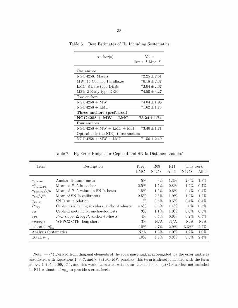
– 38 –

Table 6. Best Estimates of H0 Including Systematics

Anchor(s) Value

[km s−1 Mpc−1]

One anchor

NGC4258: Masers 72.25± 2.51

MW: 15 Cepheid Parallaxes 76.18± 2.37

LMC: 8 Late-type DEBs 72.04± 2.67

M31: 2 Early-type DEBs 74.50± 3.27

Two anchors

NGC4258 + MW 74.04± 1.93

NGC4258 + LMC 71.62± 1.78

Three anchors (preferred)

NGC4258 + MW + LMC 73.24± 1.74

Four anchors

NGC4258 + MW + LMC + M31 73.46± 1.71

Optical only (no NIR), three anchors

NGC4258 + MW + LMC 71.56± 2.49

Table 7. H0 Error Budget for Cepheid and SN Ia Distance Ladders∗

Term Description Prev. R09 R11 This work

LMC N4258 All 3 N4258 All 3

σanchor Anchor distance, mean 5% 3% 1.3% 2.6% 1.3%

σaanchorPL Mean of P–L in anchor 2.5% 1.5% 0.8% 1.2% 0.7%

σhostPL/√n Mean of P–L values in SN Ia hosts 1.5% 1.5% 0.6% 0.4% 0.4%

σSN/√n Mean of SN Ia calibrators 2.5% 2.5% 1.9% 1.2% 1.2%

σm−z SN Ia m–z relation 1% 0.5% 0.5% 0.4% 0.4%

Rσzp Cepheid reddening & colors, anchor-to-hosts 4.5% 0.3% 1.4% 0% 0.3%

σZ Cepheid metallicity, anchor-to-hosts 3% 1.1% 1.0% 0.0% 0.5%

σPL P–L slope, ∆ logP , anchor-to-hosts 4% 0.5% 0.6% 0.2% 0.5%

σWFPC2 WFPC2 CTE, long-short 3% N/A N/A N/A N/A

subtotal, σbH0

10% 4.7% 2.9% 3.3%c 2.2%

Analysis Systematics N/A 1.3% 1.0% 1.2% 1.0%

Total, σH010% 4.8% 3.3% 3.5% 2.4%

Note. — (*) Derived from diagonal elements of the covariance matrix propagated via the error matrices

associated with Equations 1, 3, 7, and 8. (a) For MW parallax, this term is already included with the term

above. (b) For R09, R11, and this work, calculated with covariance included. (c) One anchor not included

in R11 estimate of σH0to provide a crosscheck.

– 39 –

– 40 –

Fig. 1.— Uncertainties in the determination of H0. Uncertainties are squared to show their indi-

vidual contribution to the quadrature sum. These terms are given in Table 7.

– 41 –

Fig. 2.— HST observations of the host galaxies of ideal SNe Ia. The data used to observe Cepheids

in 19 SN Ia hosts and NGC4258 have been collected over 20 years with 4 cameras and over 600

orbits of HST time. 60-90 day campaigns in F555W and F814W or in F350LP were used to identify

Cepheids from their light curves with occasional reobservations years later to identify Cepheids with

P > 60 d. Near-IR follow-up observations in F160W are used to reduce the effects of host-galaxy

extinction, sensitivity to metallicity, and breaks in the P–L relation. Data sources: (1) HST

SN Ia Calibration Project, Sandage et al. (2006); (2) HST Key Project, Freedman et al. (2001);

(3) Riess et al. (2005); (4) Macri et al. (2006); and (5) Mager et al. (2013).

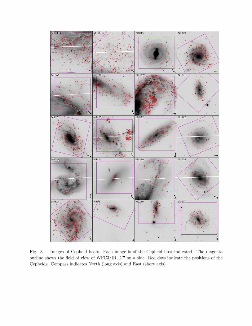
– 42 –

Fig. 3.— Images of Cepheid hosts. Each image is of the Cepheid host indicated. The magenta

outline shows the field of view of WFC3/IR, 2.′7 on a side. Red dots indicate the positions of the

Cepheids. Compass indicates North (long axis) and East (short axis).

– 43 –

0.5

0.0

-0.5

mag

-mea

n

N3021

N3370

N1309

N3982

N4639

N5584

N4038

0.5

0.0

-0.5

mag

-mea

n

N4536

N1015

N1365

N1448

N3447

N7250

N5917

0.2 0.4 0.6 0.8phase

0.5

0.0

-0.5

mag

-mea

n

N4424

0.2 0.4 0.6 0.8phase

U9391

0.2 0.4 0.6 0.8phase

N3972

0.2 0.4 0.6 0.8phase

N2442

0.2 0.4 0.6 0.8phase

M101F1

0.2 0.4 0.6 0.8phase

M101F2

0.2 0.4 0.6 0.8phase

N4258

Fig. 4.— Composite visual (F555W) or white-light (F350LP) Cepheid light curves. Each HST

Cepheid light curve with 10 < P < 80 days is plotted after subtracting the mean magnitude and

determining the phase of the observation. Two fields (F1 and F2) are shown for M101.

– 44 –

N3021 P= 44.36

Removed

Model

Residual

N3370 P= 46.59

Removed

Model

Residual

N1309 P= 41.01

Removed

Model

Residual

N3982 P= 40.44

Removed

Model

Residual

N4639 P= 41.18

Removed

Model

Residual

N5584 P= 41.75

Removed

Model

Residual

N4038 P= 43.98

Removed

Model

Residual

N4536 P= 41.67

Removed

Model

Residual

N1015 P= 50.08

Removed

Model

Residual

N1365 P= 40.72

Removed

Model

Residual

N1448 P= 40.07

Removed

Model

Residual

N3447 P= 40.54

Removed

Model

Residual

N7250 P= 68.64

Removed

Model

Residual

N5917 P= 40.05

Removed

Model

Residual

N4424 P= 36.39

Removed

Model

Residual

U9391 P= 44.89

Removed

Model

Residual

N3972 P= 53.88

Removed

Model

Residual

N2442 P= 60.74

Removed

Model

Residual

M101F1 P= 9.452

Removed

Model

Residual

N4258 P= 47.10

Removed

Model

Residual

Fig. 5.— Example WFC3 F160W Cepheid scene model for each host. A random Cepheid in the

period range of 30 < P < 70 d was selected. The four panels of each host show a 1′′ region of the

scene around each known Cepheid, the region after the Cepheid is fit and subtracted, the model of

all detected sources, and the model residuals.

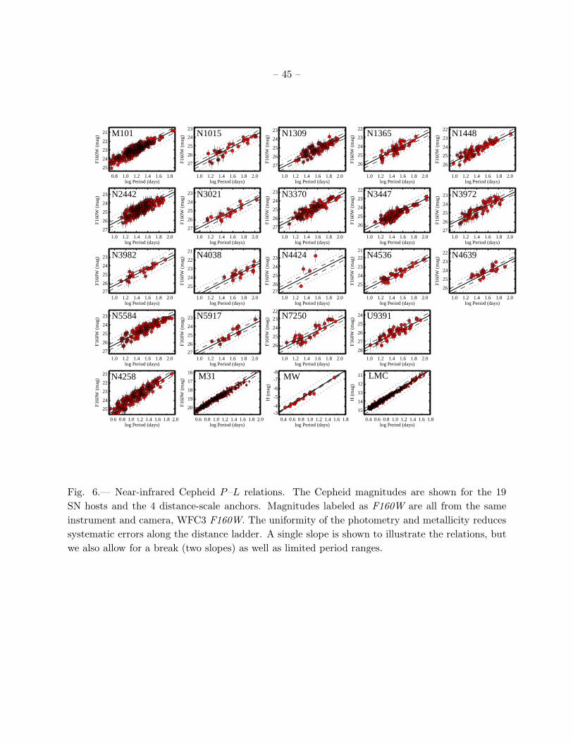
– 45 –

0.8 1.0 1.2 1.4 1.6 1.8log Period (days)

25

24

23

22

21

F160

W (

mag

) M101

1.0 1.2 1.4 1.6 1.8 2.0log Period (days)

27

26

25

24

23

F160

W (

mag

) N1015

1.0 1.2 1.4 1.6 1.8 2.0log Period (days)

27

26

25

24

23

F160

W (

mag

) N1309

1.0 1.2 1.4 1.6 1.8 2.0log Period (days)

26

25

24

23

22

F160

W (

mag

) N1365

1.0 1.2 1.4 1.6 1.8 2.0log Period (days)

26

25

24

23

22

F160

W (

mag

) N1448

1.0 1.2 1.4 1.6 1.8 2.0log Period (days)

27

26

25

24

23

F160

W (

mag

) N2442

1.0 1.2 1.4 1.6 1.8 2.0log Period (days)

27

26

25

24

23

F160

W (

mag

) N3021

1.0 1.2 1.4 1.6 1.8 2.0log Period (days)

27

26

25

24

23

F160

W (

mag

) N3370

1.0 1.2 1.4 1.6 1.8 2.0log Period (days)

26

25

24

23

22

F160

W (

mag

) N3447

1.0 1.2 1.4 1.6 1.8 2.0log Period (days)

27

26

25

24

23

F160

W (

mag

) N3972

1.0 1.2 1.4 1.6 1.8 2.0log Period (days)

27

26

25

24

23

F160

W (

mag

) N3982

1.0 1.2 1.4 1.6 1.8 2.0log Period (days)

25

24

23

22

21

F160

W (

mag

) N4038

1.0 1.2 1.4 1.6 1.8 2.0log Period (days)

27

26

25

24

23

F160

W (

mag

) N4424

1.0 1.2 1.4 1.6 1.8 2.0log Period (days)

25

24

23

22

21

F160

W (

mag

) N4536

1.0 1.2 1.4 1.6 1.8 2.0log Period (days)

26

25

24

23

22

F160

W (

mag

) N4639

1.0 1.2 1.4 1.6 1.8 2.0log Period (days)

27

26

25

24

23

F160

W (

mag

) N5584

1.0 1.2 1.4 1.6 1.8 2.0log Period (days)

27

26

25

24

23

F160

W (

mag

) N5917

1.0 1.2 1.4 1.6 1.8 2.0log Period (days)

26

25

24

23

22

F160

W (

mag

) N7250

1.0 1.2 1.4 1.6 1.8 2.0log Period (days)

28

27

26

25

24

F160

W (

mag

) U9391

0.6 0.8 1.0 1.2 1.4 1.6 1.8 2.0log Period (days)

25

24

23

22

21

F160

W (

mag

) N4258

0.6 0.8 1.0 1.2 1.4 1.6 1.8 2.0log Period (days)

20

19

18

17

16

F160

W (

mag

) M31

0.4 0.6 0.8 1.0 1.2 1.4 1.6 1.8log Period (days)

-3

-4

-5

-6

-7

-8

H (

mag

)

MW

0.4 0.6 0.8 1.0 1.2 1.4 1.6 1.8log Period (days)

15

14

13

12

11

H (

mag

)

LMC

Fig. 6.— Near-infrared Cepheid P–L relations. The Cepheid magnitudes are shown for the 19

SN hosts and the 4 distance-scale anchors. Magnitudes labeled as F160W are all from the same

instrument and camera, WFC3 F160W. The uniformity of the photometry and metallicity reduces

systematic errors along the distance ladder. A single slope is shown to illustrate the relations, but

we also allow for a break (two slopes) as well as limited period ranges.

– 46 –

6.5 7.0 7.5 8.0 8.5Distance (Mpc)

0.0

0.2

0.4

0.6

0.8

1.0no

rmal

ized

pro

babi

lity

dens

ity (

Mpc

-1)

107 MCMC TrialsHumphreys et al. (2013)

D=7.60 +/-0.17 (stat) +/-0.15 (sys)

109 MCMC TrialsD=7.54 +/-0.17 (stat) +/-0.10 (sys)

Fig. 7.— Normalized probability density function (PDF) for the maser-based distance to NGC4258.

The curve in black shows the PDF for the distance to NGC4258 based on the same multiparameter

fit of the maser data in NGC4258 from Humphreys et al. (2013) with the x-axis expanded by 18%

to match the rescaling used by H13 to account for χ2ν = 1.4. With a 100-fold increase (red curve) in

the MCMC sampling, we have reduced the 1.5% systematic error in distance from Humphreys et al.

(2013), which reflected different results with differing initial conditions using more-limited MCMC

sampling of the parameter space.

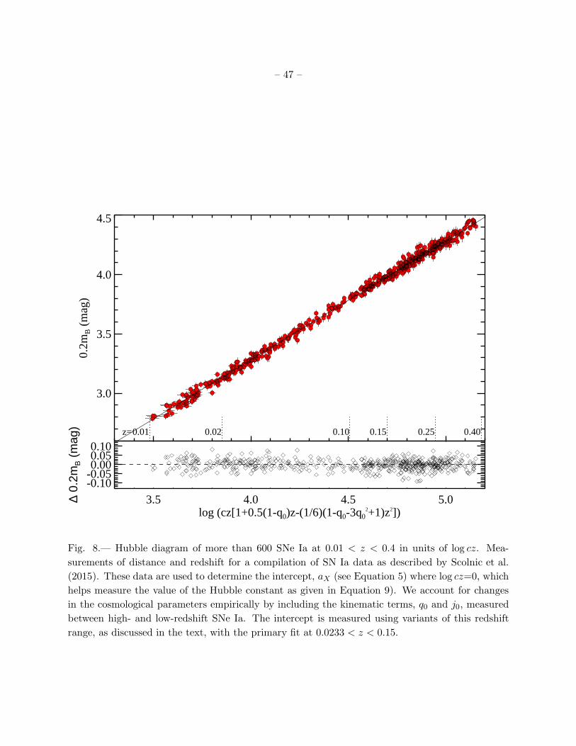
– 47 –

3.0

3.5

4.0

4.5

0.2m

B (

mag

)

0.01 0.02 0.10 0.15 0.25 0.40 z=

3.5 4.0 4.5 5.0log (cz[1+0.5(1-q0)z-(1/6)(1-q0-3q0

2+1)z2])

-0.10-0.050.000.050.10

∆ 0.

2mB (

mag

)

Fig. 8.— Hubble diagram of more than 600 SNe Ia at 0.01 < z < 0.4 in units of log cz. Mea-

surements of distance and redshift for a compilation of SN Ia data as described by Scolnic et al.

(2015). These data are used to determine the intercept, aX (see Equation 5) where log cz=0, which

helps measure the value of the Hubble constant as given in Equation 9). We account for changes

in the cosmological parameters empirically by including the kinematic terms, q0 and j0, measured

between high- and low-redshift SNe Ia. The intercept is measured using variants of this redshift

range, as discussed in the text, with the primary fit at 0.0233 < z < 0.15.

– 48 –

29

30

31

32

33C

eph

eid

mIW

(m

ag)

NGC 4258 1

2 3

4 5 6

7

8

9

10 11 12

13 14

15

16

17

18

19 1 2011fe 2 2009ig 3 2002fk 4 2012fr 5 2001el 6 2015F 7 1995al 8 1994ae 9 2012ht 10 2011by 11 1998aq 12 2007sr 13 2012cg 14 1981B 15 1990N 16 2007af 17 2005cf 18 2013dy 19 2003du

10 11 12 13SN Ia mB

0 (mag)

29

30

31

32

33

Cep

hei

d m

HW (

mag

)

1

2 3

4 5 6

7

8 9

10 11

12

13 14

15 16

17

18

19 1 M101 2 N1015 3 N1309 4 N1365 5 N1448 6 N2442 7 N3021 8 N3370 9 N3447 10 N3972 11 N3982 12 N4038 13 N4424 14 N4536 15 N4639 16 N5584 17 N5917 18 N7250 19 U9391

NGC 4258

Fig. 9.— Relative distances from Cepheids and SNe Ia. The top and bottom panels show relative

distances for 19 hosts determined from their SNe Ia and Cepheid Wesenheit optical and NIR

magnitudes, respectively. The Cepheid result for each host is an approximated distance derived

after removing that host’s SN Ia data from the full global fit for H0. The relative dispersions are

0.12 mag (top) and 0.15 mag (bottom). The maser-calibrated Cepheid distance to NGC4258 is

indicated as well as the model-fit SN Ia magnitude it would host.

– 49 –

34

36

38

40

µ (z

,H0=

73.2

,q0,

j 0)

Type Ia Supernovae → redshift(z)

29

30

31

32

33

SN I

a: m

-M (

mag

)Cepheids → Type Ia Supernovae

34 36 38 40

-0.4

0.0

0.4

∆ m

ag

SN Ia: m-M (mag)

10

15

20

25

Geometry → Cepheids

Cep

heid

: m-M

(m

ag)

Milky Way

LMC

M31

N4258

29 30 31 32 33

-0.4

0.0

0.4

∆ m

ag

Cepheid: m-M (mag)

10 15 20 25

-0.4

-0.2

0.0

0.2

0.4

-0.4

0.0

0.4

∆ m

ag

Geometry: 5 log D [Mpc] + 25

Fig. 10.— Complete distance ladder. The simultaneous agreement of pairs of geometric and

Cepheid-based distances (lower left), Cepheid and SN Ia-based distances (middle panel) and SN

and redshift-based distances provides the measurement of the Hubble constant. For each step,

geometric or calibrated distances on the x-axis serve to calibrate a relative distance indicator on

the y-axis through the determination of M or H0. Results shown are an approximation to the

global fit as discussed in the text.

– 50 –

68 70 72 74 76 78H0

0

5

10

15

# va

rian

ts

Rel

ativ

e L

ikel

ihoo

d

LMC

NGC 4258MW

M31

N4258+MW+LMCstatstat+sys

Systematicerror

Variants

N4258+MW+LMC+M31

H0 and statisticalerrors for

different anchors

Fig. 11.— Determination of systematic errors in H0 for the set of anchors used in the primary fit

(N4258, MW & LMC). By varying factors outside the global fit and its parameters such as the

assumed reddening law, its parameters, the presence of a metallicity dependence, the presence of

breaks in the P–L relations, selection of SN light curve fitter, morphology or local star formation

rate of hosts, etc. We derive a systematic error from a Gaussian fit to the variants. This error is

smaller than the indicated statistical errors.

– 51 –

0.00 0.05 0.10 0.15 0.20 0.25zmin

0.94

0.96

0.98

1.00

1.02

1.04

1.06

∆ H

\ H

H0 for zmin< z <(zmin+0.15)

Enclosed Volume (Gpc3)=

1.60 3.20 5.10 7.50 10.2

Fig. 12.— Fractional variation in H0 resulting from a progressively higher redshift (lower cosmic

variance) range used to measure the Hubble expansion, zmin < z < zmin + 0.15. Empirically

increasing zmin from 0.0233 (primary fit) to 0.25 and the maximum redshift from 0.15 (primary

fit) to 0.40 produces variations consistent with the measurement uncertainty of ± 0.004-0.006 and

the simulated uncertainty of ±0.0027 (intrinsic) from Odderskov et al. (2016). Thus a difference

between the local and global H0 of even ∼ 1% is exceedingly unlikely.

– 52 –

Fig. 13.— Local measurements of H0 compared to values predicted by CMB data in

conjunction with ΛCDM. We show 4 SN Ia-independent values selected for comparison by

Planck Collaboration et al. (2014) and their average, the primary fit from R11, its reanalysis by

Efstathiou (2014) and the results presented here. The 3.4σ difference between Planck+ΛCDM

(Planck Collaboration et al. 2016) and our result motivates the exploration of extensions to ΛCDM.

– 53 –

62 64 66 68 70 72 74H0 (km s-1 Mpc-1)

-1.2

-1.1

-1.0

-0.9

-0.8

w

Planck15+BAO+SN+H0Planck15+BAO+SN

Fig. 14.— Confidence regions determined with CosmoMC based on the data from Planck

(TT+TEB+lensing), BAO including Lyα QSOs, the JLA SN sample (Betoule et al. 2014) and

with and without our determination of H0 for the wCDM cosmological model. As shown there is a

degeneracy between w and H0 and the local measurement of H0 pulls the solution to a lower value

of w though it is still consistent with -1.

– 54 –

62 64 66 68 70 72 74H0 (km s-1 Mpc-1)

2.5

3.0

3.5

4.0

Nef

f

Planck15+BAO+SN+H0Planck15+BAO+SN

Fig. 15.— Same as Figure 14 but for the NeffCDM model. The local measurement of H0 pulls the

solution towards Neff > 3.046 which also provides a marginally better fit to the full data set than

ΛCDM.

– 55 –

1 2 3 4% error in external H0

0.02

0.04

0.06

0.08

0.10

0.12

σ (

w)

PLANCK+BAO15

PLANCK Pol+BAO15

CMB Stage IV+BAO15

This work

Fig. 16.— Constraint in the dark energy equation of state as a function of the precision of the local

determination of the Hubble constant. Past and current precision is indicated as well as a future

goal of 1%.

– 56 –

Table 8. Fits for H0

χ2dof

H0 Anc Brk Clp σ Opt PL R RV N Z γ b bl SN zm M0V av Gal

0.92 73.46 1.53 All Y 1 2.7 Y WH F 3.3 2277 Z -0.13 0.07 -3.26 0.02 -3.25 0.02 S 0.02 -19.24 0.71273 A

0.93 73.48 1.53 All Y G 2.7 Y WH F 3.3 2280 Z -0.12 0.07 -3.25 0.02 -3.25 0.02 S 0.02 -19.24 0.71273 A

0.88 72.73 1.49 All Y I 2.7 Y WH F 3.3 2280 Z -0.10 0.07 -3.31 0.02 -3.22 0.02 S 0.02 -19.27 0.71273 A

1.28 73.68 1.79 All Y G No Y WH F 3.3 2345 Z -0.10 0.08 -3.26 0.02 -3.24 0.02 S 0.02 -19.24 0.71273 A

1.10 73.67 1.66 All Y G 3.5 Y WH F 3.3 2321 Z -0.14 0.07 -3.25 0.02 -3.25 0.02 S 0.02 -19.24 0.71273 A

1.09 73.64 1.66 All Y 1 3.5 Y WH F 3.3 2320 Z -0.14 0.07 -3.25 0.02 -3.25 0.02 S 0.02 -19.24 0.71273 A

0.92 72.69 1.52 All Y I 3.5 Y WH F 3.3 2320 Z -0.09 0.07 -3.30 0.02 -3.22 0.02 S 0.02 -19.27 0.71273 A

1.11 73.21 1.66 All Y G 3.5 Y WH F 2.5 2322 Z -0.14 0.07 -3.25 0.02 -3.24 0.02 S 0.02 -19.25 0.71273 A

0.92 74.04 1.54 All Y G 2.7 Y WH C 3.3 2278 Z -0.11 0.07 -3.27 0.02 -3.27 0.02 S 0.02 -19.23 0.71273 A

0.94 73.14 1.54 All Y G 2.7 Y WH N 3.3 2278 Z -0.11 0.07 -3.24 0.02 -3.24 0.02 S 0.02 -19.25 0.71273 A

0.93 73.49 1.52 All N G 2.7 Y WH F 3.3 2280 Z -0.12 0.07 -3.25 0.01 . . . S 0.02 -19.24 0.71273 A

1.12 72.19 1.72 All 10 G 2.7 Y WH F 3.3 1318 Z -0.15 0.08 -3.26 0.03 . . . S 0.02 -19.28 0.71273 A

0.91 73.32 1.51 All 60 G 2.7 Y WH F 3.3 2180 Z -0.16 0.07 -3.25 0.01 . . . S 0.02 -19.25 0.71273 A

1.06 75.55 1.67 All Y G 2.7 Y H F 3.3 2240 Z -0.08 0.07 -3.07 0.02 -3.16 0.02 S 0.02 -19.18 0.71273 A

0.94 73.45 1.54 All Y G 2.7 Y WH F 3.3 2281 Z . . . -3.26 0.02 -3.25 0.02 S 0.02 -19.24 0.71273 A

0.93 73.60 1.53 All Y G 2.7 Y WH F 3.3 2280 Z -0.12 0.07 -3.25 0.02 -3.25 0.02 S 0.01 -19.24 0.71347 A

0.93 75.08 1.65 All Y G 2.7 Y WH F 3.3 2279 Z -0.06 0.07 -3.27 0.02 -3.25 0.02 M 0.02 -19.15 0.70326 A

0.94 74.66 1.55 All Y G 2.7 N WH F 3.3 2417 Z -0.15 0.07 -3.21 0.02 -3.26 0.02 S 0.02 -19.21 0.71273 A

0.93 73.85 1.58 All Y G 2.7 Y WH F 3.3 2280 B -0.10 0.09 -3.25 0.02 -3.25 0.02 S 0.02 -19.23 0.71273 A

0.93 73.59 1.60 All Y G 2.7 Y WH F 3.3 2280 Z -0.12 0.07 -3.25 0.02 -3.25 0.02 S 0.02 -19.24 0.71340 S

0.93 74.57 1.70 All Y G 2.7 Y WH F 3.3 2279 Z -0.06 0.07 -3.27 0.02 -3.25 0.02 M 0.02 -19.15 0.70031 S

0.93 73.76 1.66 All Y G 2.7 Y WH F 3.3 2280 Z -0.12 0.07 -3.25 0.02 -3.25 0.02 S 0.01 -19.24 0.71444 L

0.93 74.23 1.71 All Y G 2.7 Y WH F 3.3 2280 Z -0.12 0.07 -3.25 0.02 -3.25 0.02 S 0.02 -19.24 0.71719 L

0.92 73.24 1.59 NML Y 1 2.7 Y WH F 3.3 2276 Z -0.13 0.07 -3.26 0.02 -3.25 0.02 S 0.02 -19.25 0.71273 A

0.93 73.25 1.60 NML Y G 2.7 Y WH F 3.3 2279 Z -0.12 0.07 -3.25 0.02 -3.25 0.02 S 0.02 -19.25 0.71273 A

0.88 72.67 1.56 NML Y I 2.7 Y WH F 3.3 2279 Z -0.10 0.07 -3.31 0.02 -3.22 0.02 S 0.02 -19.27 0.71273 A

1.28 73.49 1.87 NML Y G No Y WH F 3.3 2344 Z -0.10 0.08 -3.26 0.02 -3.24 0.02 S 0.02 -19.24 0.71273 A

1.10 73.45 1.74 NML Y G 3.5 Y WH F 3.3 2320 Z -0.14 0.07 -3.25 0.02 -3.25 0.02 S 0.02 -19.24 0.71273 A

1.09 73.42 1.73 NML Y 1 3.5 Y WH F 3.3 2319 Z -0.14 0.07 -3.25 0.02 -3.25 0.02 S 0.02 -19.25 0.71273 A

0.92 72.62 1.59 NML Y I 3.5 Y WH F 3.3 2319 Z -0.09 0.07 -3.30 0.02 -3.22 0.02 S 0.02 -19.27 0.71273 A

1.11 73.15 1.74 NML Y G 3.5 Y WH F 2.5 2321 Z -0.14 0.07 -3.25 0.02 -3.24 0.02 S 0.02 -19.25 0.71273 A

0.92 73.33 1.59 NML Y G 2.7 Y WH C 3.3 2277 Z -0.12 0.07 -3.27 0.02 -3.27 0.02 S 0.02 -19.25 0.71273 A

0.94 73.39 1.61 NML Y G 2.7 Y WH N 3.3 2277 Z -0.11 0.07 -3.24 0.02 -3.24 0.02 S 0.02 -19.25 0.71273 A

0.93 73.26 1.59 NML N G 2.7 Y WH F 3.3 2279 Z -0.12 0.07 -3.25 0.01 . . . S 0.02 -19.25 0.71273 A

1.12 71.64 1.81 NML 10 G 2.7 Y WH F 3.3 1317 Z -0.16 0.08 -3.26 0.03 . . . S 0.02 -19.30 0.71273 A

0.91 73.06 1.58 NML 60 G 2.7 Y WH F 3.3 2179 Z -0.17 0.07 -3.25 0.01 . . . S 0.02 -19.26 0.71273 A

1.06 74.79 1.73 NML Y G 2.7 Y H F 3.3 2239 Z -0.09 0.07 -3.06 0.02 -3.17 0.02 S 0.02 -19.21 0.71273 A

0.94 73.30 1.61 NML Y G 2.7 Y WH F 3.3 2280 Z . . . -3.26 0.02 -3.25 0.02 S 0.02 -19.25 0.71273 A

0.93 73.38 1.60 NML Y G 2.7 Y WH F 3.3 2279 Z -0.12 0.07 -3.25 0.02 -3.25 0.02 S 0.01 -19.25 0.71347 A

0.93 74.89 1.72 NML Y G 2.7 Y WH F 3.3 2278 Z -0.06 0.07 -3.27 0.02 -3.25 0.02 M 0.02 -19.15 0.70326 A

0.94 74.39 1.62 NML Y G 2.7 N WH F 3.3 2416 Z -0.15 0.07 -3.21 0.02 -3.26 0.02 S 0.02 -19.22 0.71273 A

0.93 73.64 1.63 NML Y G 2.7 Y WH F 3.3 2279 B -0.11 0.09 -3.25 0.02 -3.25 0.02 S 0.02 -19.24 0.71273 A

0.93 73.37 1.66 NML Y G 2.7 Y WH F 3.3 2279 Z -0.12 0.07 -3.25 0.02 -3.25 0.02 S 0.02 -19.25 0.71340 S

0.93 74.39 1.76 NML Y G 2.7 Y WH F 3.3 2278 Z -0.06 0.07 -3.27 0.02 -3.25 0.02 M 0.02 -19.15 0.70031 S

0.93 73.54 1.73 NML Y G 2.7 Y WH F 3.3 2279 Z -0.12 0.07 -3.25 0.02 -3.25 0.02 S 0.01 -19.25 0.71444 L

– 57 –

Table 8—Continued

χ2dof

H0 Anc Brk Clp σ Opt PL R RV N Z γ b bl SN zm M0V av Gal

0.93 74.01 1.77 NML Y G 2.7 Y WH F 3.3 2279 Z -0.12 0.07 -3.25 0.02 -3.25 0.02 S 0.02 -19.25 0.71719 L

0.92 74.04 1.74 NM Y 1 2.7 Y WH F 3.3 2275 Z -0.16 0.07 -3.26 0.02 -3.25 0.02 S 0.02 -19.23 0.71273 A

0.93 74.01 1.75 NM Y G 2.7 Y WH F 3.3 2278 Z -0.14 0.07 -3.25 0.02 -3.25 0.02 S 0.02 -19.23 0.71273 A

0.87 73.67 1.71 NM Y I 2.7 Y WH F 3.3 2278 Z -0.13 0.07 -3.31 0.02 -3.22 0.02 S 0.02 -19.24 0.71273 A

1.28 74.20 2.04 NM Y G No Y WH F 3.3 2343 Z -0.12 0.08 -3.26 0.02 -3.24 0.02 S 0.02 -19.22 0.71273 A

1.10 74.30 1.90 NM Y G 3.5 Y WH F 3.3 2319 Z -0.17 0.08 -3.25 0.02 -3.25 0.02 S 0.02 -19.22 0.71273 A

1.09 74.27 1.89 NM Y 1 3.5 Y WH F 3.3 2318 Z -0.17 0.08 -3.25 0.02 -3.25 0.02 S 0.02 -19.22 0.71273 A

0.92 73.57 1.75 NM Y I 3.5 Y WH F 3.3 2318 Z -0.12 0.07 -3.30 0.02 -3.22 0.02 S 0.02 -19.24 0.71273 A

1.11 74.04 1.90 NM Y G 3.5 Y WH F 2.5 2320 Z -0.17 0.08 -3.25 0.02 -3.24 0.02 S 0.02 -19.23 0.71273 A

0.92 74.03 1.74 NM Y G 2.7 Y WH C 3.3 2277 Z -0.15 0.07 -3.28 0.02 -3.27 0.02 S 0.02 -19.23 0.71273 A

0.95 74.17 1.77 NM Y G 2.7 Y WH N 3.3 2278 Z -0.14 0.07 -3.24 0.02 -3.24 0.02 S 0.02 -19.22 0.71273 A

0.93 74.03 1.73 NM N G 2.7 Y WH F 3.3 2278 Z -0.14 0.07 -3.25 0.01 . . . S 0.02 -19.23 0.71273 A

1.12 71.36 2.17 NM 10 G 2.7 Y WH F 3.3 1316 Z -0.15 0.08 -3.26 0.03 . . . S 0.02 -19.31 0.71273 A

0.91 73.98 1.73 NM 60 G 2.7 Y WH F 3.3 2179 Z -0.22 0.08 -3.25 0.01 . . . S 0.02 -19.23 0.71273 A

1.06 75.57 1.89 NM Y G 2.7 Y H F 3.3 2239 Z -0.12 0.07 -3.07 0.02 -3.17 0.02 S 0.02 -19.18 0.71273 A

0.94 73.70 1.74 NM Y G 2.7 Y WH F 3.3 2279 Z . . . -3.26 0.02 -3.25 0.02 S 0.02 -19.24 0.71273 A

0.93 74.14 1.75 NM Y G 2.7 Y WH F 3.3 2278 Z -0.14 0.07 -3.25 0.02 -3.25 0.02 S 0.01 -19.23 0.71347 A

0.94 75.50 1.86 NM Y G 2.7 Y WH F 3.3 2278 Z -0.10 0.07 -3.27 0.02 -3.25 0.02 M 0.02 -19.14 0.70326 A

0.93 75.27 1.77 NM Y G 2.7 N WH F 3.3 2415 Z -0.19 0.07 -3.21 0.02 -3.26 0.02 S 0.02 -19.19 0.71273 A

0.93 74.57 1.83 NM Y G 2.7 Y WH F 3.3 2278 B -0.16 0.10 -3.25 0.02 -3.25 0.02 S 0.02 -19.21 0.71273 A

0.93 74.13 1.80 NM Y G 2.7 Y WH F 3.3 2278 Z -0.14 0.07 -3.25 0.02 -3.25 0.02 S 0.02 -19.23 0.71340 S

0.94 74.99 1.91 NM Y G 2.7 Y WH F 3.3 2278 Z -0.10 0.07 -3.27 0.02 -3.25 0.02 M 0.02 -19.14 0.70031 S

0.93 74.31 1.86 NM Y G 2.7 Y WH F 3.3 2278 Z -0.14 0.07 -3.25 0.02 -3.25 0.02 S 0.01 -19.23 0.71444 L

0.93 74.78 1.91 NM Y G 2.7 Y WH F 3.3 2278 Z -0.14 0.07 -3.25 0.02 -3.25 0.02 S 0.02 -19.23 0.71719 L

0.92 71.62 1.68 NL Y 1 2.7 Y WH F 3.3 2276 Z -0.18 0.07 -3.26 0.02 -3.25 0.02 S 0.02 -19.30 0.71273 A

0.93 71.86 1.70 NL Y G 2.7 Y WH F 3.3 2279 Z -0.15 0.07 -3.25 0.02 -3.25 0.02 S 0.02 -19.29 0.71273 A

0.87 71.60 1.66 NL Y I 2.7 Y WH F 3.3 2279 Z -0.13 0.07 -3.31 0.02 -3.22 0.02 S 0.02 -19.30 0.71273 A

1.28 72.14 1.98 NL Y G No Y WH F 3.3 2344 Z -0.13 0.08 -3.25 0.02 -3.24 0.02 S 0.02 -19.28 0.71273 A

1.09 72.01 1.84 NL Y G 3.5 Y WH F 3.3 2320 Z -0.18 0.07 -3.25 0.02 -3.25 0.02 S 0.02 -19.29 0.71273 A

1.09 71.99 1.83 NL Y 1 3.5 Y WH F 3.3 2319 Z -0.18 0.07 -3.25 0.02 -3.25 0.02 S 0.02 -19.29 0.71273 A

0.92 71.51 1.70 NL Y I 3.5 Y WH F 3.3 2319 Z -0.12 0.07 -3.29 0.02 -3.22 0.02 S 0.02 -19.30 0.71273 A

1.10 71.77 1.84 NL Y G 3.5 Y WH F 2.5 2321 Z -0.17 0.07 -3.24 0.02 -3.25 0.02 S 0.02 -19.29 0.71273 A

0.92 71.80 1.69 NL Y G 2.7 Y WH C 3.3 2278 Z -0.18 0.07 -3.27 0.02 -3.27 0.02 S 0.02 -19.29 0.71273 A

0.94 71.86 1.71 NL Y G 2.7 Y WH N 3.3 2277 Z -0.15 0.07 -3.24 0.02 -3.24 0.02 S 0.02 -19.29 0.71273 A

0.93 71.84 1.69 NL N G 2.7 Y WH F 3.3 2279 Z -0.15 0.07 -3.25 0.01 . . . S 0.02 -19.29 0.71273 A

1.13 71.21 1.86 NL 10 G 2.7 Y WH F 3.3 1319 Z -0.19 0.08 -3.26 0.03 . . . S 0.02 -19.31 0.71273 A

0.91 71.42 1.67 NL 60 G 2.7 Y WH F 3.3 2180 Z -0.24 0.08 -3.25 0.01 . . . S 0.02 -19.31 0.71273 A

1.06 73.32 1.83 NL Y G 2.7 Y H F 3.3 2240 Z -0.13 0.07 -3.06 0.02 -3.17 0.02 S 0.02 -19.25 0.71273 A

0.93 72.25 1.70 NL Y G 2.7 Y WH F 3.3 2280 Z . . . -3.26 0.02 -3.25 0.02 S 0.02 -19.28 0.71273 A

0.93 71.98 1.70 NL Y G 2.7 Y WH F 3.3 2279 Z -0.15 0.07 -3.25 0.02 -3.25 0.02 S 0.01 -19.29 0.71347 A

0.93 73.53 1.81 NL Y G 2.7 Y WH F 3.3 2279 Z -0.11 0.07 -3.26 0.02 -3.25 0.02 M 0.02 -19.19 0.70326 A

0.93 72.78 1.71 NL Y G 2.7 N WH F 3.3 2417 Z -0.21 0.07 -3.21 0.02 -3.26 0.02 S 0.02 -19.26 0.71273 A

0.93 72.24 1.70 NL Y G 2.7 Y WH F 3.3 2279 B -0.22 0.10 -3.25 0.02 -3.25 0.02 S 0.02 -19.28 0.71273 A

0.93 71.97 1.75 NL Y G 2.7 Y WH F 3.3 2279 Z -0.15 0.07 -3.25 0.02 -3.25 0.02 S 0.02 -19.29 0.71340 S

0.93 73.03 1.85 NL Y G 2.7 Y WH F 3.3 2279 Z -0.11 0.07 -3.26 0.02 -3.25 0.02 M 0.02 -19.19 0.70031 S

0.93 72.15 1.81 NL Y G 2.7 Y WH F 3.3 2279 Z -0.15 0.07 -3.25 0.02 -3.25 0.02 S 0.01 -19.29 0.71444 L

– 58 –

Table 8—Continued

χ2dof

H0 Anc Brk Clp σ Opt PL R RV N Z γ b bl SN zm M0V av Gal

0.93 72.60 1.85 NL Y G 2.7 Y WH F 3.3 2279 Z -0.15 0.07 -3.25 0.02 -3.25 0.02 S 0.02 -19.29 0.71719 L

0.92 74.15 1.82 M+L Y 1 2.7 Y WH F 3.3 2275 Z -0.14 0.07 -3.26 0.02 -3.25 0.02 S 0.02 -19.22 0.71273 A

0.93 74.27 1.84 M+L Y G 2.7 Y WH F 3.3 2278 Z -0.11 0.07 -3.25 0.02 -3.25 0.02 S 0.02 -19.22 0.71273 A

0.88 72.84 1.75 M+L Y I 2.7 Y WH F 3.3 2278 Z -0.10 0.07 -3.31 0.02 -3.22 0.02 S 0.02 -19.26 0.71273 A

1.28 74.51 2.15 M+L Y G No Y WH F 3.3 2343 Z -0.10 0.08 -3.26 0.02 -3.24 0.02 S 0.02 -19.21 0.71273 A

1.10 74.43 1.99 M+L Y G 3.5 Y WH F 3.3 2319 Z -0.14 0.07 -3.25 0.02 -3.25 0.02 S 0.02 -19.22 0.71273 A

1.09 74.40 1.99 M+L Y 1 3.5 Y WH F 3.3 2318 Z -0.14 0.07 -3.25 0.02 -3.25 0.02 S 0.02 -19.22 0.71273 A

0.92 72.92 1.80 M+L Y I 3.5 Y WH F 3.3 2318 Z -0.09 0.07 -3.30 0.02 -3.22 0.02 S 0.02 -19.26 0.71273 A

1.11 73.95 1.99 M+L Y G 3.5 Y WH F 2.5 2320 Z -0.14 0.07 -3.25 0.02 -3.24 0.02 S 0.02 -19.23 0.71273 A

0.92 74.45 1.83 M+L Y G 2.7 Y WH C 3.3 2276 Z -0.12 0.07 -3.27 0.02 -3.27 0.02 S 0.02 -19.22 0.71273 A

0.94 74.35 1.85 M+L Y G 2.7 Y WH N 3.3 2275 Z -0.11 0.07 -3.24 0.02 -3.24 0.02 S 0.02 -19.22 0.71273 A

0.93 74.28 1.82 M+L N G 2.7 Y WH F 3.3 2278 Z -0.11 0.07 -3.25 0.01 . . . S 0.02 -19.22 0.71273 A

1.12 72.70 2.18 M+L 10 G 2.7 Y WH F 3.3 1316 Z -0.15 0.08 -3.26 0.03 . . . S 0.02 -19.27 0.71273 A

0.90 74.29 1.81 M+L 60 G 2.7 Y WH F 3.3 2176 Z -0.14 0.07 -3.25 0.01 . . . S 0.02 -19.22 0.71273 A

1.06 75.96 1.99 M+L Y G 2.7 Y H F 3.3 2237 Z -0.09 0.07 -3.06 0.02 -3.16 0.02 S 0.02 -19.17 0.71273 A

0.93 74.40 1.84 M+L Y G 2.7 Y WH F 3.3 2279 Z . . . -3.26 0.02 -3.25 0.02 S 0.02 -19.22 0.71273 A

0.93 74.39 1.84 M+L Y G 2.7 Y WH F 3.3 2278 Z -0.11 0.07 -3.25 0.02 -3.25 0.02 S 0.01 -19.22 0.71347 A

0.93 75.96 1.95 M+L Y G 2.7 Y WH F 3.3 2277 Z -0.06 0.07 -3.26 0.02 -3.25 0.02 M 0.02 -19.12 0.70326 A

0.93 75.65 1.86 M+L Y G 2.7 N WH F 3.3 2414 Z -0.15 0.07 -3.21 0.02 -3.26 0.02 S 0.02 -19.18 0.71273 A

0.93 74.94 1.89 M+L Y G 2.7 Y WH F 3.3 2278 B -0.13 0.09 -3.25 0.02 -3.25 0.02 S 0.02 -19.20 0.71273 A

0.93 74.38 1.89 M+L Y G 2.7 Y WH F 3.3 2278 Z -0.11 0.07 -3.25 0.02 -3.25 0.02 S 0.02 -19.22 0.71340 S

0.93 75.44 1.99 M+L Y G 2.7 Y WH F 3.3 2277 Z -0.06 0.07 -3.26 0.02 -3.25 0.02 M 0.02 -19.12 0.70031 S

0.93 74.56 1.95 M+L Y G 2.7 Y WH F 3.3 2278 Z -0.11 0.07 -3.25 0.02 -3.25 0.02 S 0.01 -19.22 0.71444 L

0.93 75.03 1.99 M+L Y G 2.7 Y WH F 3.3 2278 Z -0.11 0.07 -3.25 0.02 -3.25 0.02 S 0.02 -19.22 0.71719 L

1.04 72.25 2.38 N Y 1 2.7 Y WH F 3.3 1485 Z -0.16 0.08 -3.10 0.03 -3.46 0.05 S 0.02 -19.28 0.71273 A

1.05 72.52 2.39 N Y G 2.7 Y WH F 3.3 1486 Z -0.14 0.08 -3.10 0.03 -3.45 0.05 S 0.02 -19.27 0.71273 A

0.89 73.31 2.43 N Y I 2.7 Y WH F 3.3 1486 Z -0.14 0.07 -3.21 0.03 -3.40 0.05 S 0.02 -19.25 0.71273 A

1.48 72.78 2.56 N Y G No Y WH F 3.3 1540 Z -0.13 0.09 -3.11 0.04 -3.46 0.06 S 0.02 -19.26 0.71273 A

1.26 72.93 2.48 N Y G 3.5 Y WH F 3.3 1522 Z -0.17 0.08 -3.09 0.04 -3.47 0.06 S 0.02 -19.26 0.71273 A

1.25 72.97 2.48 N Y 1 3.5 Y WH F 3.3 1520 Z -0.18 0.08 -3.09 0.04 -3.47 0.06 S 0.02 -19.26 0.71273 A

0.96 73.12 2.44 N Y I 3.5 Y WH F 3.3 1520 Z -0.13 0.08 -3.18 0.04 -3.42 0.05 S 0.02 -19.25 0.71273 A

1.26 73.03 2.49 N Y G 3.5 Y WH F 2.5 1522 Z -0.18 0.08 -3.08 0.04 -3.47 0.06 S 0.02 -19.26 0.71273 A

1.06 72.20 2.38 N Y G 2.7 Y WH C 3.3 1486 Z -0.14 0.08 -3.11 0.03 -3.44 0.06 S 0.02 -19.28 0.71273 A

1.04 72.61 2.39 N Y G 2.7 Y WH N 3.3 1485 Z -0.14 0.08 -3.09 0.03 -3.45 0.05 S 0.02 -19.27 0.71273 A

1.06 71.57 2.35 N N G 2.7 Y WH F 3.3 1485 Z -0.15 0.08 -3.23 0.02 . . . S 0.02 -19.30 0.71273 A

1.12 70.99 2.39 N 10 G 2.7 Y WH F 3.3 1203 Z -0.15 0.08 -3.11 0.04 . . . S 0.02 -19.32 0.71273 A

1.04 71.09 2.35 N 60 G 2.7 Y WH F 3.3 1388 Z -0.23 0.08 -3.25 0.03 . . . S 0.02 -19.32 0.71273 A

1.11 74.35 2.45 N Y G 2.7 Y H F 3.3 1470 Z -0.12 0.07 -2.90 0.03 -3.14 0.06 S 0.02 -19.22 0.71273 A

1.05 72.21 2.38 N Y G 2.7 Y WH F 3.3 1487 Z . . . -3.09 0.03 -3.45 0.05 S 0.02 -19.28 0.71273 A

1.05 72.64 2.39 N Y G 2.7 Y WH F 3.3 1486 Z -0.14 0.08 -3.10 0.03 -3.45 0.05 S 0.01 -19.27 0.71347 A

1.06 74.16 2.50 N Y G 2.7 Y WH F 3.3 1487 Z -0.10 0.08 -3.11 0.03 -3.44 0.06 M 0.02 -19.18 0.70326 A

1.05 72.90 2.39 N Y G 2.7 N WH F 3.3 1626 Z -0.17 0.07 -3.05 0.03 -3.46 0.05 S 0.02 -19.26 0.71273 A

1.05 72.52 2.39 N Y G 2.7 Y WH F 3.3 1486 B -0.20 0.11 -3.10 0.03 -3.45 0.05 S 0.02 -19.27 0.71273 A

1.05 72.63 2.43 N Y G 2.7 Y WH F 3.3 1486 Z -0.14 0.08 -3.10 0.03 -3.45 0.05 S 0.02 -19.27 0.71340 S

1.06 73.66 2.53 N Y G 2.7 Y WH F 3.3 1487 Z -0.10 0.08 -3.11 0.03 -3.44 0.06 M 0.02 -19.18 0.70031 S

1.05 72.80 2.48 N Y G 2.7 Y WH F 3.3 1486 Z -0.14 0.08 -3.10 0.03 -3.45 0.05 S 0.01 -19.27 0.71444 L

– 59 –

Table 8—Continued

χ2dof

H0 Anc Brk Clp σ Opt PL R RV N Z γ b bl SN zm M0V av Gal

1.05 73.26 2.52 N Y G 2.7 Y WH F 3.3 1486 Z -0.14 0.08 -3.10 0.03 -3.45 0.05 S 0.02 -19.27 0.71719 L

0.92 76.18 2.17 M Y 1 2.7 Y WH F 3.3 2274 Z -0.18 0.07 -3.26 0.02 -3.25 0.02 S 0.02 -19.17 0.71273 A

0.93 76.12 2.18 M Y G 2.7 Y WH F 3.3 2277 Z -0.15 0.07 -3.25 0.02 -3.25 0.02 S 0.02 -19.17 0.71273 A

0.87 74.58 2.08 M Y I 2.7 Y WH F 3.3 2277 Z -0.14 0.07 -3.31 0.02 -3.22 0.02 S 0.02 -19.21 0.71273 A

1.28 76.30 2.55 M Y G No Y WH F 3.3 2342 Z -0.13 0.08 -3.26 0.02 -3.24 0.02 S 0.02 -19.16 0.71273 A

1.10 76.46 2.37 M Y G 3.5 Y WH F 3.3 2318 Z -0.17 0.08 -3.25 0.02 -3.25 0.02 S 0.02 -19.16 0.71273 A

1.09 76.40 2.36 M Y 1 3.5 Y WH F 3.3 2317 Z -0.17 0.08 -3.25 0.02 -3.25 0.02 S 0.02 -19.16 0.71273 A

0.92 74.64 2.13 M Y I 3.5 Y WH F 3.3 2317 Z -0.12 0.07 -3.29 0.02 -3.22 0.02 S 0.02 -19.21 0.71273 A

1.10 75.94 2.36 M Y G 3.5 Y WH F 2.5 2319 Z -0.17 0.08 -3.25 0.02 -3.24 0.02 S 0.02 -19.17 0.71273 A

0.92 76.27 2.17 M Y G 2.7 Y WH C 3.3 2276 Z -0.16 0.07 -3.27 0.02 -3.27 0.02 S 0.02 -19.16 0.71273 A

0.94 76.21 2.20 M Y G 2.7 Y WH N 3.3 2276 Z -0.14 0.07 -3.23 0.02 -3.24 0.02 S 0.02 -19.16 0.71273 A

0.93 76.15 2.16 M N G 2.7 Y WH F 3.3 2277 Z -0.15 0.07 -3.25 0.01 . . . S 0.02 -19.17 0.71273 A

1.12 74.42 3.70 M 10 G 2.7 Y WH F 3.3 1315 Z -0.16 0.08 -3.26 0.03 . . . S 0.02 -19.22 0.71273 A

0.91 76.38 2.15 M 60 G 2.7 Y WH F 3.3 2176 Z -0.23 0.08 -3.25 0.01 . . . S 0.02 -19.16 0.71273 A

1.06 77.83 2.37 M Y G 2.7 Y H F 3.3 2238 Z -0.12 0.07 -3.06 0.02 -3.17 0.02 S 0.02 -19.12 0.71273 A

0.93 75.64 2.16 M Y G 2.7 Y WH F 3.3 2278 Z . . . -3.26 0.02 -3.25 0.02 S 0.02 -19.18 0.71273 A

0.93 76.25 2.18 M Y G 2.7 Y WH F 3.3 2277 Z -0.15 0.07 -3.25 0.02 -3.25 0.02 S 0.01 -19.17 0.71347 A

0.94 77.64 2.29 M Y G 2.7 Y WH F 3.3 2277 Z -0.10 0.07 -3.26 0.02 -3.25 0.02 M 0.02 -19.08 0.70326 A

0.93 77.84 2.22 M Y G 2.7 N WH F 3.3 2413 Z -0.20 0.07 -3.21 0.02 -3.26 0.02 S 0.02 -19.12 0.71273 A

0.93 77.77 2.41 M Y G 2.7 Y WH F 3.3 2277 B -0.23 0.10 -3.25 0.02 -3.25 0.02 S 0.02 -19.12 0.71273 A

0.93 76.24 2.22 M Y G 2.7 Y WH F 3.3 2277 Z -0.15 0.07 -3.25 0.02 -3.25 0.02 S 0.02 -19.17 0.71340 S

0.94 77.11 2.32 M Y G 2.7 Y WH F 3.3 2277 Z -0.10 0.07 -3.26 0.02 -3.25 0.02 M 0.02 -19.08 0.70031 S

0.93 76.42 2.28 M Y G 2.7 Y WH F 3.3 2277 Z -0.15 0.07 -3.25 0.02 -3.25 0.02 S 0.01 -19.17 0.71444 L

0.93 76.91 2.32 M Y G 2.7 Y WH F 3.3 2277 Z -0.15 0.07 -3.25 0.02 -3.25 0.02 S 0.02 -19.17 0.71719 L

0.92 72.04 2.56 L Y 1 2.7 Y WH F 3.3 2275 Z -0.18 0.07 -3.26 0.02 -3.25 0.02 S 0.02 -19.29 0.71273 A

0.93 72.27 2.58 L Y G 2.7 Y WH F 3.3 2278 Z -0.15 0.07 -3.25 0.02 -3.25 0.02 S 0.02 -19.28 0.71273 A

0.87 70.97 2.49 L Y I 2.7 Y WH F 3.3 2278 Z -0.14 0.07 -3.31 0.02 -3.22 0.02 S 0.02 -19.32 0.71273 A

1.28 72.58 2.88 L Y G No Y WH F 3.3 2343 Z -0.13 0.08 -3.25 0.03 -3.24 0.02 S 0.02 -19.27 0.71273 A

1.09 72.30 2.72 L Y G 3.5 Y WH F 3.3 2319 Z -0.18 0.08 -3.25 0.02 -3.25 0.02 S 0.02 -19.28 0.71273 A

1.09 72.28 2.72 L Y 1 3.5 Y WH F 3.3 2318 Z -0.17 0.08 -3.25 0.02 -3.25 0.02 S 0.02 -19.28 0.71273 A

0.92 71.09 2.53 L Y I 3.5 Y WH F 3.3 2318 Z -0.12 0.07 -3.29 0.02 -3.23 0.02 S 0.02 -19.32 0.71273 A

1.10 71.82 2.71 L Y G 3.5 Y WH F 2.5 2320 Z -0.17 0.08 -3.24 0.02 -3.25 0.02 S 0.02 -19.29 0.71273 A

0.91 72.34 2.57 L Y G 2.7 Y WH C 3.3 2276 Z -0.17 0.07 -3.27 0.02 -3.27 0.02 S 0.02 -19.28 0.71273 A

0.94 72.31 2.59 L Y G 2.7 Y WH N 3.3 2276 Z -0.14 0.07 -3.24 0.02 -3.24 0.02 S 0.02 -19.28 0.71273 A

0.93 72.25 2.57 L N G 2.7 Y WH F 3.3 2278 Z -0.15 0.07 -3.25 0.01 . . . S 0.02 -19.28 0.71273 A

1.12 72.20 2.75 L 10 G 2.7 Y WH F 3.3 1316 Z -0.16 0.08 -3.26 0.03 . . . S 0.02 -19.28 0.71273 A

0.91 71.74 2.54 L 60 G 2.7 Y WH F 3.3 2178 Z -0.23 0.08 -3.25 0.01 . . . S 0.02 -19.30 0.71273 A

1.06 73.82 2.74 L Y G 2.7 Y H F 3.3 2238 Z -0.12 0.07 -3.06 0.02 -3.17 0.02 S 0.02 -19.23 0.71273 A

0.93 73.07 2.58 L Y G 2.7 Y WH F 3.3 2279 Z . . . -3.26 0.02 -3.25 0.02 S 0.02 -19.26 0.71273 A

0.93 72.39 2.58 L Y G 2.7 Y WH F 3.3 2278 Z -0.15 0.07 -3.25 0.02 -3.25 0.02 S 0.01 -19.28 0.71347 A

0.93 74.05 2.69 L Y G 2.7 Y WH F 3.3 2278 Z -0.11 0.07 -3.26 0.02 -3.25 0.02 M 0.02 -19.18 0.70326 A

0.93 73.43 2.61 L Y G 2.7 N WH F 3.3 2414 Z -0.20 0.07 -3.21 0.02 -3.26 0.02 S 0.02 -19.25 0.71273 A

0.93 72.93 2.57 L Y G 2.7 Y WH F 3.3 2278 B -0.22 0.10 -3.25 0.02 -3.25 0.02 S 0.02 -19.26 0.71273 A

0.93 72.38 2.62 L Y G 2.7 Y WH F 3.3 2278 Z -0.15 0.07 -3.25 0.02 -3.25 0.02 S 0.02 -19.28 0.71340 S

0.93 73.55 2.71 L Y G 2.7 Y WH F 3.3 2278 Z -0.11 0.07 -3.26 0.02 -3.25 0.02 M 0.02 -19.18 0.70031 S

0.93 72.56 2.66 L Y G 2.7 Y WH F 3.3 2278 Z -0.15 0.07 -3.25 0.02 -3.25 0.02 S 0.01 -19.28 0.71444 L

– 60 –

Table 8—Continued

χ2dof

H0 Anc Brk Clp σ Opt PL R RV N Z γ b bl SN zm M0V

av Gal

0.93 73.02 2.70 L Y G 2.7 Y WH F 3.3 2278 Z -0.15 0.07 -3.25 0.02 -3.25 0.02 S 0.02 -19.28 0.71719 L

0.92 74.50 2.87 A Y 1 2.7 Y WH F 3.3 2275 Z -0.18 0.07 -3.26 0.02 -3.25 0.02 S 0.02 -19.21 0.71273 A

0.93 74.53 2.89 A Y G 2.7 Y WH F 3.3 2278 Z -0.15 0.07 -3.25 0.02 -3.25 0.02 S 0.02 -19.21 0.71273 A

0.87 73.00 2.75 A Y I 2.7 Y WH F 3.3 2278 Z -0.14 0.07 -3.31 0.02 -3.22 0.02 S 0.02 -19.26 0.71273 A

1.28 74.53 3.39 A Y G No Y WH F 3.3 2343 Z -0.13 0.08 -3.25 0.03 -3.24 0.02 S 0.02 -19.21 0.71273 A

1.09 74.69 3.14 A Y G 3.5 Y WH F 3.3 2319 Z -0.17 0.08 -3.25 0.02 -3.25 0.02 S 0.02 -19.21 0.71273 A

1.09 74.66 3.14 A Y 1 3.5 Y WH F 3.3 2318 Z -0.17 0.08 -3.25 0.02 -3.25 0.02 S 0.02 -19.21 0.71273 A

0.92 73.00 2.82 A Y I 3.5 Y WH F 3.3 2318 Z -0.12 0.07 -3.29 0.02 -3.23 0.02 S 0.02 -19.26 0.71273 A

1.10 73.38 3.10 A Y G 3.5 Y WH F 2.5 2320 Z -0.17 0.08 -3.24 0.02 -3.25 0.02 S 0.02 -19.25 0.71273 A

0.92 77.66 3.00 A Y G 2.7 Y WH C 3.3 2277 Z -0.18 0.07 -3.27 0.02 -3.27 0.02 S 0.02 -19.12 0.71273 A

0.94 71.80 2.81 A Y G 2.7 Y WH N 3.3 2277 Z -0.14 0.07 -3.23 0.02 -3.24 0.02 S 0.02 -19.29 0.71273 A

0.93 74.50 2.88 A N G 2.7 Y WH F 3.3 2278 Z -0.15 0.07 -3.25 0.01 . . . S 0.02 -19.21 0.71273 A

1.12 74.40 3.19 A 10 G 2.7 Y WH F 3.3 1316 Z -0.16 0.08 -3.26 0.03 . . . S 0.02 -19.22 0.71273 A

0.91 74.70 2.86 A 60 G 2.7 Y WH F 3.3 2178 Z -0.23 0.08 -3.25 0.01 . . . S 0.02 -19.21 0.71273 A

1.06 79.49 3.29 A Y G 2.7 Y H F 3.3 2239 Z -0.12 0.07 -3.06 0.02 -3.17 0.02 S 0.02 -19.07 0.71273 A

0.93 74.04 2.87 A Y G 2.7 Y WH F 3.3 2279 Z . . . -3.26 0.02 -3.25 0.02 S 0.02 -19.23 0.71273 A

0.93 74.66 2.89 A Y G 2.7 Y WH F 3.3 2278 Z -0.15 0.07 -3.25 0.02 -3.25 0.02 S 0.01 -19.21 0.71347 A

0.93 75.97 3.00 A Y G 2.7 Y WH F 3.3 2278 Z -0.10 0.07 -3.26 0.02 -3.25 0.02 M 0.02 -19.12 0.70326 A

0.93 75.98 2.94 A Y G 2.7 N WH F 3.3 2413 Z -0.19 0.07 -3.21 0.02 -3.26 0.02 S 0.02 -19.17 0.71273 A

0.93 76.11 3.09 A Y G 2.7 Y WH F 3.3 2278 B -0.22 0.10 -3.25 0.02 -3.25 0.02 S 0.02 -19.17 0.71273 A

0.93 74.65 2.93 A Y G 2.7 Y WH F 3.3 2278 Z -0.15 0.07 -3.25 0.02 -3.25 0.02 S 0.02 -19.21 0.71340 S

0.93 75.46 3.02 A Y G 2.7 Y WH F 3.3 2278 Z -0.10 0.07 -3.26 0.02 -3.25 0.02 M 0.02 -19.12 0.70031 S

0.93 74.83 2.97 A Y G 2.7 Y WH F 3.3 2278 Z -0.15 0.07 -3.25 0.02 -3.25 0.02 S 0.01 -19.21 0.71444 L

0.93 75.30 3.01 A Y G 2.7 Y WH F 3.3 2278 Z -0.15 0.07 -3.25 0.02 -3.25 0.02 S 0.02 -19.21 0.71719 L

0.91 71.96 1.47 All Y 1 2.7 Y WI F 3.3 3138 Z -0.20 0.05 -3.17 0.02 -3.40 0.02 S 0.02 -19.29 0.71273 A

0.91 71.74 1.54 NML Y 1 2.7 Y WI F 3.3 3137 Z -0.20 0.05 -3.17 0.02 -3.40 0.02 S 0.02 -19.30 0.71273 A

1.09 72.41 2.26 N Y 1 2.7 Y WI F 3.3 2364 Z -0.19 0.05 -3.08 0.03 -4.14 0.05 S 0.02 -19.28 0.71273 A

Note. — H0: error listed from fit for M0X in eq 9 or m0

x,4258 in eq 4 only. Anc: Anchors used; N=N4258 Masers, M=MW Parallaxes,

L=LMC DEBs, NML=primary fit using all three, A=NML+M31 DEBs. Brk: Break in P–Lrelation; Y=two-slope solution, N=single-slope

solution, 10=single slope restricted to P > 10 d, 60=single slope restrcited to P < 60 d. Clp: Clipping procedure; G=global, I=individual,

1=Global but removing single largest outlier at a time. σ: clipping threshold. Opt: optical completeness required, Y=Yes, N=No. PL: Form

of P–Lrelation used; WH : NIR Wesenheit; H NIR without extinction correction; WI : Optical Wesenheit. R: reddening law; F99=Fitzpatrick

(1999), CCM=Cardelli et al. (1989), N=Nataf et al. (2016). RV : Extinction-law parameter. N: Number of Cepheids fit. Z: Metallicity scale;

Z=traditional R23 method (Zaritsky et al. 1994), B=Te method (Bresolin 2011). γ: change in Wesenheit mag per dex in log(O/H). b: slope

of P–L for all P in no-break variants or for P >10 d for two-slope variants. bl: slope of P–L for P <10 d (when applicable). SN: light-curve

fitter; S=SALT, M=MLCS2k2. zm: minimum z used in SN Hubble diagram (0.02 stands for 0.0233). M0V : SN absolute magnitude (X stands

for B or V depending on the SN fitter, see text). aX : intercept of SN Hubble diagram (X=B or V ). Gal: SN host galaxy sample; A=All,

S=Spiral, L=high LSF.

– 61 –

REFERENCES

Addison, G. E., Huang, Y., Watts, D. J., et al. 2015, ArXiv e-prints, arXiv:1511.00055

Argon, A. L., Greenhill, L. J., Reid, M. J., Moran, J. M., & Humphreys, E. M. L. 2007, ApJ, 659,

1040

Aubourg, E., Bailey, S., Bautista, J. E., et al. 2015, Phys. Rev. D, 92, 123516

Beaton, R. L., Freedman, W. L., Madore, B. F., et al. 2016, ArXiv e-prints, arXiv:1604.01788

Becker, M. R., Desmond, H., Rozo, E., Marshall, P., & Rykoff, E. S. 2015, ArXiv e-prints,

arXiv:1507.07523

Benedict, G. F., McArthur, B. E., Feast, M. W., et al. 2007, AJ, 133, 1810

Bennett, C. L., Larson, D., Weiland, J. L., & Hinshaw, G. 2014, ApJ, 794, 135

Bennett, C. L., Larson, D., Weiland, J. L., et al. 2013, ApJS, 208, 20

Betoule, M., Kessler, R., Guy, J., et al. 2014, A&A, 568, A22

Bhardwaj, A., Kanbur, S. M., Macri, L. M., et al. 2016, MNRAS, 457, 1644

Bird, J. C., Stanek, K. Z., & Prieto, J. L. 2009, ApJ, 695, 874

Birrer, S., Amara, A., & Refregier, A. 2015, ArXiv e-prints, arXiv:1511.03662

Bonamente, M., Joy, M. K., LaRoque, S. J., et al. 2006, ApJ, 647, 25

Bonanos, A. Z., & Stanek, K. Z. 2003, ApJ, 591, L111

Bresolin, F. 2011, ApJ, 729, 56

Brust, C., Kaplan, D. E., & Walters, M. T. 2013, Journal of High Energy Physics, 12, 58

Calabrese, E., Hlozek, R. A., Battaglia, N., et al. 2013, Phys. Rev. D, 87, 103012

Cardelli, J. A., Clayton, G. C., & Mathis, J. S. 1989, ApJ, 345, 245

Carrick, J., Turnbull, S. J., Lavaux, G., & Hudson, M. J. 2015, MNRAS, 450, 317

Casertano, S., Anderson, A. G. R. J., Anderson, R. I., et al. 2015, ArXiv e-prints, arXiv:1512.09371

Cuesta, A. J., Verde, L., Riess, A., & Jimenez, R. 2015, MNRAS, 448, 3463

Dalcanton, J. J., Williams, B. F., Lang, D., et al. 2012, ApJS, 200, 18

Darling, J. 2011, ApJ, 732, L2

– 62 –

Di Benedetto, G. P. 2005, MNRAS, 357, 174

Dvorkin, C., Wyman, M., Rudd, D. H., & Hu, W. 2014, Phys. Rev. D, 90, 083503

Efstathiou, G. 2014, MNRAS, 440, 1138

Ferrarese, L., Silbermann, N. A., Mould, J. R., et al. 2000, PASP, 112, 177

Fiorentino, G., Clementini, G., Marconi, M., et al. 2012, Ap&SS, 341, 143

Fitzpatrick, E. L. 1999, PASP, 111, 63

Fitzpatrick, E. L., Ribas, I., Guinan, E. F., et al. 2002, ApJ, 564, 260

Fitzpatrick, E. L., Ribas, I., Guinan, E. F., Maloney, F. P., & Claret, A. 2003, ApJ, 587, 685

Freedman, W. L., & Madore, B. F. 2010, ARA&A, 48, 673

Freedman, W. L., Madore, B. F., Scowcroft, V., et al. 2012, ApJ, 758, 24

Freedman, W. L., Madore, B. F., Gibson, B. K., et al. 2001, ApJ, 553, 47

Gao, F., Braatz, J. A., Reid, M. J., et al. 2016, ApJ, 817, 128

Guinan, E. F., Fitzpatrick, E. L., Dewarf, L. E., et al. 1998, ApJ, 509, L21

Guy, J., Astier, P., Nobili, S., Regnault, N., & Pain, R. 2005, A&A, 443, 781

Guy, J., Sullivan, M., Conley, A., et al. 2010, A&A, 523, A7

Hanson, R. B. 1979, MNRAS, 186, 875

Herrnstein, J. R., Moran, J. M., Greenhill, L. J., et al. 1999, Nature, 400, 539

Hicken, M., Wood-Vasey, W. M., Blondin, S., et al. 2009a, ApJ, 700, 1097

Hicken, M., Challis, P., Jha, S., et al. 2009b, ApJ, 700, 331

Hinshaw, G., Larson, D., Komatsu, E., et al. 2013, ApJS, 208, 19

Hu, W. 2005, in Astronomical Society of the Pacific Conference Series, Vol. 339, Observing Dark

Energy, ed. S. C. Wolff & T. R. Lauer, 215

Humphreys, E. M. L., Argon, A. L., Greenhill, L. J., Moran, J. M., & Reid, M. J. 2005, in

Astronomical Society of the Pacific Conference Series, Vol. 340, Future Directions in High

Resolution Astronomy, ed. J. Romney & M. Reid, 466

Humphreys, E. M. L., Reid, M. J., Greenhill, L. J., Moran, J. M., & Argon, A. L. 2008, ApJ, 672,

800

– 63 –

Humphreys, E. M. L., Reid, M. J., Moran, J. M., Greenhill, L. J., & Argon, A. L. 2013, ApJ, 775,

13

Jha, S., Riess, A. G., & Kirshner, R. P. 2007, ApJ, 659, 122

Jones, D. O., Riess, A. G., & Scolnic, D. M. 2015, ApJ, 812, 31

Kaluzny, J., Stanek, K. Z., Krockenberger, M., et al. 1998, AJ, 115, 1016

Kelly, P. L., Hicken, M., Burke, D. L., Mandel, K. S., & Kirshner, R. P. 2010, ApJ, 715, 743

Kodric, M., Riffeser, A., Seitz, S., et al. 2015, ApJ, 799, 144

Laidler, V., Boffi, F., Barlow, T., & et al. 2008

Lampeitl, H., Smith, M., Nichol, R. C., et al. 2010, ApJ, 722, 566

Leavitt, H. S., & Pickering, E. C. 1912, Harvard College Observatory Circular, 173, 1

Leistedt, B., Peiris, H. V., & Verde, L. 2014, Physical Review Letters, 113, 041301

Livio, M., & Riess, A. G. 2013, Physics Today, 66, 41

Macri, L. M., Ngeow, C.-C., Kanbur, S. M., Mahzooni, S., & Smitka, M. T. 2015, AJ, 149, 117

Macri, L. M., Stanek, K. Z., Bersier, D., Greenhill, L. J., & Reid, M. J. 2006, ApJ, 652, 1133

Madore, B. F. 1982, ApJ, 253, 575

Madore, B. F., & Freedman, W. L. 1991, PASP, 103, 933

Mager, V. A., Madore, B. F., & Freedman, W. L. 2013, ApJ, 777, 79

Nataf, D. M., Gonzalez, O. A., Casagrande, L., et al. 2016, MNRAS, 456, 2692

Ngeow, C.-C., & Kanbur, S. M. 2005, MNRAS, 360, 1033

Odderskov, I., Koksbang, S. M., & Hannestad, S. 2016, J. Cosmology Astropart. Phys., 2, 001

Paczynski, B., & Sasselov, D. 1997, in Variable Stars and the Astrophysical Returns of the Mi-

crolensing Surveys, ed. R. Ferlet, J.-P. Maillard, & B. Raban, 309

Persson, S. E., Madore, B. F., Krzeminski, W., et al. 2004, AJ, 128, 2239

Pietrzynski, G., Graczyk, D., Gieren, W., et al. 2013, Nature, 495, 76

Planck Collaboration, Ade, P. A. R., Aghanim, N., et al. 2014, A&A, 571, A16

—. 2015, ArXiv e-prints, arXiv:1502.01589

– 64 –

Planck Collaboration, Aghanim, N., Ashdown, M., et al. 2016, ArXiv e-prints, arXiv:1605.02985

Ribas, I., Fitzpatrick, E. L., Maloney, F. P., Guinan, E. F., & Udalski, A. 2002, ApJ, 574, 771

Ribas, I., Jordi, C., Vilardell, F., et al. 2005, ApJ, 635, L37

Riess, A. G. 2010, First On-orbit Measurements of the WFC3-IR Count-rate Non-Linearity, Tech.

rep.

—. 2011, An Independent Determination of WFC3-IR Zeropoints and Count Rate Non-Linearity

from 2MASS Asterisms, Tech. rep.

Riess, A. G., Casertano, S., Anderson, J., MacKenty, J., & Filippenko, A. V. 2014, ApJ, 785, 161

Riess, A. G., Fliri, J., & Valls-Gabaud, D. 2012, ApJ, 745, 156

Riess, A. G., Li, W., Stetson, P. B., et al. 2005, ApJ, 627, 579

Riess, A. G., Strolger, L., Casertano, S., et al. 2007, ApJ, 659, 98

Riess, A. G., Macri, L., Casertano, S., et al. 2009a, ApJ, 699, 539

Riess, A. G., Macri, L., Li, W., et al. 2009b, ApJS, 183, 109

Riess, A. G., Macri, L., Casertano, S., et al. 2011, ApJ, 730, 119

Rigault, M., Copin, Y., Aldering, G., et al. 2013, A&A, 560, A66

Rigault, M., Aldering, G., Kowalski, M., et al. 2015, ApJ, 802, 20

Romaniello, M., Primas, F., Mottini, M., et al. 2008, A&A, 488, 731

Saha, A., Sandage, A., Labhardt, L., et al. 1996, ApJ, 466, 55

Sakai, S., Ferrarese, L., Kennicutt, Jr., R. C., & Saha, A. 2004, ApJ, 608, 42

Sandage, A., Tammann, G. A., Saha, A., et al. 2006, ApJ, 653, 843

Scolnic, D., & Kessler, R. 2016, ApJ, 822, L35

Scolnic, D., Rest, A., Riess, A., et al. 2014, ApJ, 795, 45

Scolnic, D., Casertano, S., Riess, A., et al. 2015, ApJ, 815, 117

Senchyna, P., Johnson, L. C., Dalcanton, J. J., et al. 2015, ApJ, 813, 31

Sorce, J. G., Tully, R. B., & Courtois, H. M. 2012, ApJ, 758, L12

Soszynski, I., Poleski, R., Udalski, A., et al. 2008, Acta Astron., 58, 163

– 65 –

Spergel, D. N., Flauger, R., & Hlozek, R. 2015, Phys. Rev. D, 91, 023518

Stetson, P. B. 1987, PASP, 99, 191

—. 1996, PASP, 108, 851

Story, K. T., Reichardt, C. L., Hou, Z., et al. 2013, ApJ, 779, 86

Sullivan, M., Conley, A., Howell, D. A., et al. 2010, MNRAS, 406, 782

Suyu, S. H., Treu, T., Blandford, R. D., et al. 2012, ArXiv e-prints, arXiv:1202.4459

Suyu, S. H., Auger, M. W., Hilbert, S., et al. 2013, ApJ, 766, 70

van Leeuwen, F., Feast, M. W., Whitelock, P. A., & Laney, C. D. 2007, MNRAS, 379, 723

Vilardell, F., Ribas, I., Jordi, C., Fitzpatrick, E. L., & Guinan, E. F. 2010, A&A, 509, A70

Wagner-Kaiser, R., Sarajedini, A., Dalcanton, J. J., Williams, B. F., & Dolphin, A. 2015, MNRAS,

451, 724

Weinberg, S. 2013, Physical Review Letters, 110, 241301

Wyman, M., Rudd, D. H., Vanderveld, R. A., & Hu, W. 2014, Physical Review Letters, 112, 051302

Zaritsky, D., Kennicutt, Jr., R. C., & Huchra, J. P. 1994, ApJ, 420, 87

This preprint was prepared with the AAS LATEX macros v5.2.