1 AE Proceedings of the 18th Int. AMME Conference, 3-5 April, 2018

18th International Conference on Applied Mechanics and Mechanical Engineering.

Military Technical College Kobry El-Kobbah,

Cairo, Egypt.

A 14 DEGREES OF FREEDOM VEHICLE DYNAMICS MODEL TO

PREDICT THE BEHAVIOR OF A GOLF CAR

M. S. Ibrahim1, M. Abdelaziz2, A. Elmarhoomy3 and M. Ghoniema4

ABSTRACT A14 Degrees Of Freedom vehicle handling dynamics model is presented and implemented using MATLAB/SIMULINK software. The model is used to predict the behavior of a golf car in different steering conditions. This work is focusing on the vehicle heading modeling as a part of “implementation and control of an autonomous car project” adopted by Autotronics Research Lab (ARL). The vehicle handling related degrees of freedom are calculated. The vehicle yaw rate and lateral acceleration for step and sinusoidal steering wheel excitation are computed to predict the heading of the vehicle. The model results are verified against similar work studying the steering and handling behavior of different cars. The results show good agreement with the literature results. KEY WORDS Vehicle Dynamics and Modeling.

-----------------------------------------------------------------------------------------------------------------

1 Demonstrator, Dept. of Physics and Mathematics, Faculty of Engineering, Ain Shams University, Cairo, Egypt.

2 Assistant professor, Dept. of Automotive, Faculty of Engineering, Ain Shams University, Cairo, Egypt.

3 Professor, Dept. of Physics & Mathematics, Faculty of Engineering, Ain Shams University, Cairo, Egypt.

4 Assistant professor, Dept. of mechatronics, Faculty of Engineering, Ain Shams University, Cairo, Egypt.

2 AE Proceedings of the 18th Int. AMME Conference, 3-5 April, 2018

NOMENCLATURE a��� Linear acceleration of c.g. (m/s2)

a������ Acceleration of ij (front right, front left, rear right and rear left) center of the unsprung mass in F2 (m/s2) �� Suspension damping coefficient (N.s/m)

����/ ����/ ���� Longitudinal/lateral/vertical force of ij (front right, front left, rear right and rear left) tire (N)

F������/F������ Longitudinal / lateral force at ij (front right, front left, rear right and rear left) tire-ground contact patch in F1 (N)

F�����/F����� Longitudinal / lateral force at ij (front right, front left, rear right and rear left) tire-ground contact patch in F2 (N) F���� Vertical tire force in F1 (N) F��� Vertical suspension force in F2 (N) F�/F�/F� Total longitudinal/lateral/vertical force acting on the vehicle (N) � Gravitational acceleration (m/s2) ℎ Height of center of gravity (m) �� Roll moment of inertia (kg.m2) �� Pitch moment of inertia (kg.m2) �� Yaw moment of inertia (kg.m2) �� Wheel’s rotational moment of inertia (kg.m2) � Suspension spring stiffness (N/m) � Tire stiffness (N/m)

L Wheel base (! = #$ + #&) (m) #$ Distance from front axle to center of gravity (m) #& Distance from rear axle to center of gravity (m) #� Instantaneous length of strut (m)

M�)* /M�)* /M�)* Moments acting on c.g. in x/y/z directions due to forces on front right corner (N.m)

M�), /M�), /M�), Moments acting on c.g. in x/y/z directions due to forces on front left corner (N.m)

M�** /M�** /M�** Moments acting on c.g. in x/y/z directions due to forces on rear right corner (N.m)

M�*, /M�*, /M�*, Moments acting on c.g. in x/y/z directions due to forces on rear left corner (N.m) - Vehicle sprung mass (kg) -� Tire mass (kg)

.�� Effective rolling radius of ij (front right, front left, rear right and rear left) tire (m) ./ Nominal tire radius (m)

.�0��/1 Position vector of center of ij (front right, front left, rear right and rear left) unsprung mass with respect to the c.g. (m)

.�2��/1 Position vector of ij (front right, front left, rear right and rear left) tire-ground contact patch with respect to the c.g. (m) 3 Steering ratio 4 Track width (m) 45/46 Driving/Braking torque (N.m) 7��1 Linear Velocity of c.g. (m/s) 8�/8�/8� Longitudinal/Lateral/Vertical velocity of c.g. (m/s) 7��0���9 Velocity of the center of ij (front right, front left, rear right and

3 AE Proceedings of the 18th Int. AMME Conference, 3-5 April, 2018

rear left) unsprung mass in F2 (m/s)

80���/80���/80��� Longitudinal/Lateral/Vertical velocity of the center of ij (front right, front left, rear right and rear left) unsprung mass (m/s)

7��2���9� Velocity of the center of ij (front right, front left, rear right and rear left) tire-ground contact patch in F1 (m/s)

7��2���9 Velocity of the center of ij (front right, front left, rear right and rear left) tire-ground contact patch in F2 (m/s)

82���/82���/82��� Longitudinal/Lateral/Vertical velocity of ij (front right, front left, rear right and rear left) tire-ground patch (m/s) :��� Angular velocity of vehicle body (rad/s) :�/:�/:� Roll/Pitch/Yaw angular velocity of vehicle body (rad/s)

:�� ij (front right, front left, rear right and rear left) tire rotational speed (rad/s)

;��� ij (front right, front left, rear right and rear left) suspension spring compression (m) ;�/ Initial suspension spring compression (m)

;��� ij (front right, front left, rear right and rear left) tire spring compression (m) ;�/ Initial tire spring compression (m) </=/> Pitch/Roll/Yaw angle (rad) ? Steering wheel steer angle (rad) ?$&/?$@ Front right/left tire steer angle (rad)

� ij (front right, front left, rear right and rear left) tire longitudinal slip � ij (front right, front left, rear right and rear left) tire lateral slip

INTRODUCTION In last years the topic of autonomous vehicle became very popular and attractive in automotive industry market. In near future, the autonomous vehicle will replace the cars we know nowadays. The idea behind the autonomous car is to replace the human driver with a combination of sensors and electronic components that control the motion of the car. To do that, a reliable vehicle dynamics model must be developed to predict the vehicle response and can be used as a base to develop the controllers. This prediction can enhance the driving controller decisions in any situation {ex: path tracking, lane change, obstacle avoidance, etc.}. Many publications presented vehicle dynamics models where each differs in complexity and the applied application. As it seems, there is always a tradeoff between the complexity of the vehicle dynamic model and the computational power, therefore a lot effort is exerted in order to minimize the computational power without the compromise of the prediction accuracy of the car heading. In Ref. [1], the author used a bicycle model to develop a two degrees of freedom (lateral velocity and yaw rate) vehicle model that is used in studying the effect of steering, lateral disturbance ,traction and braking on vehicle lateral dynamics. In[2],the author used a 3 DOF (longitudinal, lateral and yaw) vehicle model to control an electric 4-wheel drive vehicle lateral stability. In[3], the author used a 3 DOF (longitudinal, lateral and yaw) in estimation of tire-road frictional coefficient for four-wheel driving and four-wheel steering electric ground vehicles. In [4], the author

4 AE Proceedings of the 18th Int. AMME Conference, 3-5 April, 2018

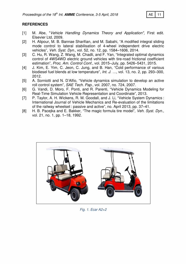
derived a 6-DOF nonlinear vehicle dynamics model, coded a related VBA (Visual Basic for Applications) and compared the model results with a simpler 3 DOF dynamics model. In [5],the author used a 14 DOF vehicle model to develop an Active Roll Control (ARC) system .In[6], the author presented a 14 DOF vehicle model for on-board applications and used the model in Hardware in the loop configuration (HIL) to verify the stability of the system. In[7], the author used different vehicle models (14-DOF & 8-DOF) to predict roll behavior and study the effect of simplifying model equations on roll response. In this paper, the vehicle of interest is an electric golf car shown in Fig.1 with the parameters estimated in Table 1. A derivation of 14 DOF vehicle dynamics model has been presented. The considered degrees of freedom are:

• Longitudinal, lateral and vertical velocities of c.g. (center of gravity) of the sprung mass.

• Roll, pitch, yaw of the sprung mass.

• The rotational speed of each tire.

• The vertical velocity of each tire.

A Simulink model is developed based on the derived equations of motion and hence different maneuvers have been tested. MODEL DESCRIPTION Kinematics Coordinate systems Two moving coordinate systems are used as shown in Fig.2, first coordinate system (F1) is attached to tire-ground contact point with coordinate axes (;�, D�, E�) and unit

vectors (F�, H�, IJ�) are obtained by rotating the inertial frame X,Y,Z with the yaw angle > about the Z-axis giving a rotation matrix:

KL = M NOP(>) PRS(>) 0−PRS(>) NOP(>) 00 0 1W ( 1 )

The second coordinate system (F2) (attached to c.g. of the vehicle with coordinate

axes (;, D, E) and unit vectors (F, H, IJ) is obtained by two successive rotations of F1, first with the pitch angle θ about the y-axis giving a rotation matrix:

KY = MNOP(<) 0 −PRS(<)0 1 0PRS(<) 0 NOP(<) W ( 2 )

And then with the roll angle = about the x-axis giving a rotation matrix:

KZ = M1 0 00 NOP(=) PRS(=)0 −PRS(=) NOP(=)W ( 3 )

5 AE Proceedings of the 18th Int. AMME Conference, 3-5 April, 2018

Velocities

Figure 3 shows top view schematic of the vehicle, let the linear velocity of c.g.(7��1) and the angular velocity of the vehicle body (:���) are: 7��1 = 8�F + 8�H + 8�IJ ( 4 )

:��� = :�F + :�H + :�IJ ( 5 )

Then the velocity of the center of the ij unsprung mass (7��0���9) and the velocity of

the ij center of tire contact patch (7��2���9) can be obtained from the velocity of c.g. as

follow: 7��0���9 = 7��1 + :��� × .�0��/1 ( 6 )

7��2���9 = 7��1 + :��� × .�2��/1 ( 7 )

Where ij represents front right (fr), front left (fl), rear right (rr) &rear left (rl). Accelerations The acceleration of c.g. (\�1) is obtained by differentiating the velocity of c.g. with respect to time as follow: \�1 = 5

5� ]7��1^ = 55� (71) + :��� × 7��1 = ]8_� + :�8� − :�8�^F + (8_� − :�8� + :�8�)H + (8_� +:�8� − :�8�)IJ ( 8 )

Similarly, the acceleration of the center of ij unsprung mass in F2 (\�0���9) is given

by: \�0���9 = 5

5� ]7��0���9^ = 55� ]70���9^ + :��� × 7��0���9 = ]8_0��� + :�80��� − :�80���^F +(8_0��� − :�80��� + :�80���)H + (8_0��� + :�80��� − :�80���)IJ ( 9 )

Note that in last equation the terms 80��� , 80��� are calculated from (6) while 80��� is

calculated from (52) as we will see. 2-Kinetics Steering mechanism The steering mechanism used is “Ackerman steering” with front right steering angle (?$&) and front left steering angle (?$@), Where:

?$& = `\S�� a b(b/ �cd(ef))g(h/)i ( 10 )

6 AE Proceedings of the 18th Int. AMME Conference, 3-5 April, 2018

?$@ = `\S�� a b(b/ �cd(ef))�(h/)i ( 11 )

Tire model The tire model used here is Pacejka’s model [8] with longitudinal and lateral slips

(j��,k��) defined as:

j�� = lmn∗&mn�(pqrmn∗1/�]smn^gpqtmn∗��d]smn^)(pqrmn∗1/�]smn^gpqtmn∗��d]smn^) ( 12 )

k�� = `\S�� upqtmnpqrmnv − ?�� ( 13 )

Where:

7��2���9� = KZKY7��2���9 = 82���F� + 82���H� + 82���IJ� ( 14 )

By using the tire model with slip ratios defined above we can calculate longitudinal and lateral tire forces ( ����, ����), and hence we can get the longitudinal and lateral

forces at ground contact patch in F1 ( 2����9�, 2����9�) as follow:

2����9� = ���� NOP]?��^ − ����PRS(?��) ( 15 )

2����9� = ���� PRS]?��^ + ����NOP(?��) ( 16 )

The tire and suspension in each corner are modeled as shown in Fig.4, so the vertical tire force ( 2����9�) can be calculated as follow:

2����9� = �� ∗ ;��� ( 17 )

where: ;_��� = −80����9� ( 18 )

With initial values obtained from static conditions as follow:

;�/$& = ;�/$@ = wx∗2∗ yz{∗|}g(x~∗2)�~� ( 19 )

;�/&& = ;�/&@ = ux∗2∗ y�{∗|vg(x~∗2)�~z ( 20 )

And to get these forces in F2 ( �2���9) we use matrix transformations as follow:

7 AE Proceedings of the 18th Int. AMME Conference, 3-5 April, 2018

�2���9 = KYhKZh �2���9� ( 21 )

Then the total forces (external and inertia forces) acting on ;, D, E directions (F�,F�,F�) are:

� = ∑( 2����9 −-�\0���) + 4-�� PRS(<) + -� PRS(<) ( 22 )

� = ∑( 2����9 −-�\0���) − 4-�� PRS(=) NOP(<) − -� PRS(=) NOP(<) ( 23 )

� = ∑] �����9^ − -� NOP(=) NOP(<) ( 24 )

where (m�a����) / (m�a����) represent the longitudinal/lateral inertia force in each tire

and �����9 is the vertical force at the suspension (Fig.4) and equal:

�����9 = �� ∗ ;��� + ��� ∗ ;_��� ( 25 )

where: ;_��� = 80��� − 8���� ( 26 )

With initial values: ;�/$& = ;�/$@ = x∗2∗@z∗b∗��� ( 27 )

;�/&& = ;�/&@ = x∗2∗@�∗b∗��z ( 28 )

Where 80��� is calculated from (52) and 8���� can be obtained from the following

relations: 8��$& = 8� − #$*:� − h ∗ :� ( 29 )

8��$@ = 8� − #$*:� + h ∗ :� ( 30 )

8��&& = 8� + #&*:� − h ∗ :� ( 31 )

8��&@ = 8� + #&*:� + h ∗ :� ( 32 )

And the moments acting on c.g. on ;, D, E directions (��$& , ��$& , ��$& ) due to

forces at front right corner can be calculated as follow: ��$& = 2�$&�9 ∗ ]#�$& + .$&^ − ]-�\0�$& +-�� PRS(=) NOP(<)^ ∗ #�$& − ��$&�9 ∗ h ( 33 )

��$& = − 2�$&�9 ∗ ]#�$& + .$&^ + ]-�\0�$& −-�� PRS(<)^ ∗ #�$& − ��$&�9 ∗ #$ ( 34 )

8 AE Proceedings of the 18th Int. AMME Conference, 3-5 April, 2018

��$& = ( 2�$&�9 −-�\0�$& +-�� PRS(<)) ∗ h + ] 2�$&�9 −-�\0�$& −-�� PRS(=) NOP(<)^ ∗ #$ ( 35 )

Where .$& = &���~�z1/�(Z)1/�(Y) ( 36 )

#�$& = ℎ − .� + ;�/$& − ;�$& + ;�/$& ( 37 )

Similarly, moments due to forces at remaining corners are: Front left: ��$@ = 2�$@�9 ∗ ]#�$@ + .$@^ − ]-�\0�$@ +-�� PRS(=) NOP(<)^ ∗ #�$@ + ��$@�9 ∗ h ( 38 )

��$@ = − 2�$@�9 ∗ ]#�$@ + .$@^ + ]-�\0�$@ −-�� PRS(<)^ ∗ #�$@ − ��$@�9 ∗ #$ ( 39 )

��$@ = (− 2�$@�9 +-�\0�$@ −-�� PRS(<)) ∗ h + ] 2�$@�9 −-�\0�$@ −-�� PRS(=) NOP(<)^ ∗ #$ ( 40 )

Rear right: ��&& = 2�&&�9 ∗ (#�&& + .&&) − ]-�\0�&& +-�� PRS(=) NOP(<)^ ∗ #�&& − ��&&�9 ∗ h ( 41 )

��&& = − 2�&&�9 ∗ (#�&& + .&&) + (-�\0�&& −-�� PRS(<)) ∗ #�&& + ��&&�9 ∗ #& ( 42 )

��&& = ( 2�&&�9 −-�\0�&& +-�� PRS(<)) ∗ h + ]− 2�&&�9 +-�\0�&& +-�� PRS(=) NOP(<)^ ∗ #& ( 43 )

Rear left: ��&@ = 2�&@�9 ∗ (#�&@ + .&@) − ]-�\0�&@ +-�� PRS(=) NOP(<)^ ∗ #�&@ + ��&@�9 ∗ h ( 44 )

��&@ = − 2�&@�9 ∗ (#�&@ + .&@) + (-�\0�&@ −-�� PRS(<)) ∗ #�&@ + ��&@�9 ∗ #& ( 45 )

��&@ = (− 2�&@�9 +-�\0�&@ −-�� PRS(<)) ∗ h + ]− 2�&@�9 +-�\0�$& +-�� PRS(=) NOP(<)^ ∗ #& ( 46 )

After defining the acceleration of c.g., all forces and moments acting on it. By direct application of newton’s laws, we can get the equations represent the 6 DOF of the body as follow: 8_� = �

x ( �) − :�8� + :�8� ( 47 )

8_� = �x ] �^ − :�8� + :�8� ( 48 )

9 AE Proceedings of the 18th Int. AMME Conference, 3-5 April, 2018

8_� = �x ( �) − :�8� +:�8� (49)

:_ � = ��r∑���� ( 50 )

:_� = ��t∑���� ( 51 )

:_ � = ���∑���� ( 52 )

And by applying Newton’s law again at z direction of the center of the unsprung mass we can get the four equations represent the 4 DOF for unsprung mass vertical velocity as follow: 8_0��� = �

x~ { 2����9 −-�� NOP(=) NOP(<) − ��;��� − ���;_��� −-�]80���:� − 80���:�^} ( 53 )

The remaining equations which represent the 4 DOF of wheels spin (Fig.5) can be calculated as follow: :��_ = h�mn�h�mn�9~rmn∗&mn�� ( 54 )

Equations from (47) to (54) represent the equations of motion for the 14 DOF vehicle model. MODEL IMPLEMENTATION As mentioned earlier the model is developed using MATLAB/SIMULINK program as shown in Fig.6. The inputs for the model are the driving torque, the braking torque and the steering wheel angle. The model was divided into 8 subsystems. First one “steering mechanism” contains equations which convert the steering wheel steer angle into front right and front left tire steer angle. The second block “Tires” contains the magic formula equations [8].The third block “Body” contains equations of the sprung mass . The forth block “wheels spin “contains equations that calculate the rotating speed of each tire. The remaining blocks contain the equations of each corner (front right, front left, rear right and rear left).

RESULTS Three steering inputs are tested: a 45o step steer, a 45o sinusoidal steer with period of 5 seconds and J-turn maneuver all at a speed of 30 km/hr (as the scope of this paper is a slow moving golf car that will be later used as an autonomous car in a current running project) .

10 AE Proceedings of the 18th Int. AMME Conference, 3-5 April, 2018

Step Steer The results for 45o step steer at 30 km/hr are shown in figures from Fig.7 to Fig.12. Fig.7 shows the step steer angle (in degrees) Vs. time (in seconds). Fig.8 shows the yaw rate (in deg/sec) Vs. time (in seconds) and it can be seen that when the steering angle was zero, the yaw rate was also zero but when the steering angle has a constant value, the yaw rate saturated at a constant value. Fig.9 shows the roll angle (in deg) Vs. time (in seconds). Fig.10 shows the lateral acceleration Vs. time. Fig.11 shows the path of c.g. of the vehicle where the vehicle started to move in straight line (when the steering angle was zero) and then moved in a circular path (when the steering angle took a constant value) .Fig.12 shows the normal force acting on each tire (in Newtons) and it can be seen that when there was no steering, the vertical forces had a constant value (equal to weight distribution on each tire) but where the vehicle started to steer, there was a load transfer between right and left tires . The results show a good agreement with the results in [7]. Sinusoidal Steer The results for 45osinusoidal steer with period of 5 seconds at 30 km/hr are shown in figures from Fig.13 to Fig.18. Fig.13 shows the sinusoidal steer angle (in degrees) Vs. time (in seconds). Fig.14 shows the yaw rate (in deg/sec) Vs. time and it can be seen that the yaw rate took sinusoidal shape with the same period of input steer. Fig.15 shows the roll angle (in deg) Vs. time (in seconds). Fig.16 shows the lateral acceleration Vs. time. Fig.17 shows the path of c.g. of the vehicle where the vehicle was continually changing its direction (as expected). Fig.18 shows the normal force acting on each tire (in Newtons) with average value in each tire equal to weight distribution in that tire. The results show a good agreement with the results in [6]. J-turn maneuver The results for J-turn maneuver at 30 km/hr are shown in figures from Fig.19 to Fig.23. Fig.19 shows the steering wheel steer angle (in degrees) Vs. time (in seconds). Fig.20 shows the yaw rate (in deg/sec) Vs. time. Fig.21 shows the roll angle (in deg) Vs. time (in seconds). Fig.22 shows the lateral acceleration Vs. time.Fig.23 shows the normal force acting on each tire (in Newtons) with average value in each tire equal to weight distribution in that tire. The results show a good agreement with the results in [7]. CONCLUSIONS A 14 DOF vehicle dynamics model was presented and full equations of the model were derived. The model was implemented in SIMULINK. The model was tested for an electric vehicle with three steering input scenarios, 45o step steer, 45o sinusoidal steer and J-turn maneuver. The results were presented and the deduced response for each case was verified according to the literature listed in [6] and [7]. This model can be used as a baseline model for vehicle heading due to steering input.

11 AE Proceedings of the 18th Int. AMME Conference, 3-5 April, 2018

REFERENCES [1] M. Abe, "Vehicle Handling Dynamics Theory and Application", First edit.

Elsevier Ltd, 2009. [2] H. Alipour, M. B. Bannae Sharifian, and M. Sabahi, “A modified integral sliding

mode control to lateral stabilisation of 4-wheel independent drive electric vehicles”, Veh. Syst. Dyn., vol. 52, no. 12, pp. 1584–1606, 2014.

[3] C. Hu, R. Wang, Z. Wang, M. Chadli, and F. Yan, “Integrated optimal dynamics control of 4WS4WD electric ground vehicles with tire-road frictional coefficient estimation”, Proc. Am. Control Conf., vol. 2015–July, pp. 5426–5431, 2015.

[4] J. Kim, E. Yim, C. Jeon, C. Jung, and B. Han, “Cold performance of various biodiesel fuel blends at low temperature”, Int. J. …, vol. 13, no. 2, pp. 293–300, 2012.

[5] A. Sorniotti and N. D’Alfio, “Vehicle dynamics simulation to develop an active roll control system”, SAE Tech. Pap., vol. 2007, no. 724, 2007.

[6] G. Vandi, D. Moro, F. Ponti, and R. Parenti, “Vehicle Dynamics Modeling for Real-Time Simulation Vehicle Representation and Coordinate”, 2013.

[7] P. Taylor, A. H. Wickens, R. M. Goodall, and J. Li, “Vehicle System Dynamics : International Journal of Vehicle Mechanics and Re-evaluation of the limitations of the railway wheelset : passive and active”, no. April 2013, pp. 37–41.

[8] H. B. Pacejka and E. Bakker, “The magic formula tire model”, Veh. Syst. Dyn., vol. 21, no. 1, pp. 1–18, 1992.

Fig. 1. Ecar A2+2

12 AE Proceedings of the 18th Int. AMME Conference, 3-5 April, 2018

Fig. 2 . Coordinate systems.

Fig. 3 . Schematic of vehicle (top view).

Fig. 4 . Suspension and tire model at ij corner.

13 AE Proceedings of the 18th Int. AMME Conference, 3-5 April, 2018

Fig. 5 . Tire rotational model.

Fig. 6 .SIMULINK block diagram.

14 AE Proceedings of the 18th Int. AMME Conference, 3-5 April, 2018

Fig. 7 . Steering wheel angle vs. time.

Fig. 8 .Yaw rate vs. time.

Fig. 9 .Roll angle vs.time.

15 AE Proceedings of the 18th Int. AMME Conference, 3-5 April, 2018

Fig. 10 .Lateral acceleration vs. time.

Fig. 11 . Path of c.g. of the vehicle.

16 AE Proceedings of the 18th Int. AMME Conference, 3-5 April, 2018

Fig. 12 . Normal force on each tire.

Fig. 13 . Steering wheel angle vs. time.

17 AE Proceedings of the 18th Int. AMME Conference, 3-5 April, 2018

Fig. 14 . Yaw rate vs. time.

Fig. 15 . Roll angle vs.time.

Fig. 16 . Lateral acceleration vs. time.

18 AE Proceedings of the 18th Int. AMME Conference, 3-5 April, 2018

Fig. 17 . Path of c.g. of tire.

Fig. 18 . Normal force on each tire.

19 AE Proceedings of the 18th Int. AMME Conference, 3-5 April, 2018

Fig. 19 . Steering wheel angle vs. time.

Fig. 20. Yaw rate vs. time.

Fig. 21. Roll angle vs.time.

20 AE Proceedings of the 18th Int. AMME Conference, 3-5 April, 2018

Fig. 22 . Lateral acceleration vs. time.

Fig. 23 . Normal force on each tire.

21 AE Proceedings of the 18th Int. AMME Conference, 3-5 April, 2018

Table 1. Vehicle parameters.

Parameter ValueValueValueValue ParameterParameterParameterParameter ValueValueValueValue

- (kg) 503 �$ (N/m) 35000

��(kg.m2) 900 ��$ (N.s/m) 2500

��(kg.m2) 2000 �&(N/m) 30000

��(kg.m2) 2000 ��&(N.s/m) 2000

#$(m) .5 -�(kg) 20

#&(m) 1.12 �$ , �& (N/m) 200000

ℎ (m) .75 ./(m) .2286

4 (m) 1 ��(kg.m2) 1