9789814401166_0001.pdf
38
Chapter 1 Preliminaries 1.1 Induction Let N = {0, 1, 2,...} be the set of natural numbers. Suppose that S is a subset of N with the following two properties: first 0 ∈ S, and second, whenever n ∈ S, then n +1 ∈ S as well. Then, invoking the Induction Principle (IP) we can conclude that S = N. We shall use the IP with a more convenient notation; let P be a property of natural numbers, in other words, P is a unary relation such that P(i) is either true or false. The relation P may be identified with a set S P in the obvious way, i.e., i ∈ S P iff P(i) is true. For example, if P is the property of being prime, then P(2) and P(3) are true, but P(6) is false, and S P = {2, 3, 5, 7, 11,...}. Using this notation the IP may be stated as: [P(0) ∧∀n(P(n) → P(n + 1))] →∀mP(m), (1.1) for any (unary) relation P over N. In practice, we use (1.1) as follows: first we prove that P(0) holds (this is the basis case). Then we show that ∀n(P(n) → P(n + 1)) (this is the induction step). Finally, using (1.1) and modus ponens, we conclude that ∀mP(m). As an example, let P be the assertion “the sum of the first i odd numbers equals i 2 .” We follow the convention that the sum of an empty set of numbers is zero; thus P(0) holds as the set of the first zero odd numbers is an empty set. P(1) is true as 1 = 1 2 , and P(3) is also true as 1+3+5 = 9 = 3 2 . We want to show that in fact ∀mP(m) i.e., P is always true, and so S P = N. Notice that S P = N does not mean that all numbers are odd—an ob- viously false assertion. We are using the natural numbers to index odd numbers, i.e., o 1 =1,o 2 =3,o 3 =5,o 4 =7,..., and our induction is over this indexing (where o i is the i-th odd number, i.e., o i =2i - 1). That is, we are proving that for all i ∈ N, o 1 + o 2 + o 3 + ··· + o i = i 2 ; our assertion 1 An Introduction to the Analysis of Algorithms Downloaded from www.worldscientific.com by NATIONAL UNITED UNIVERSITY on 02/26/15. For personal use only.
-
Upload
christopher-williamson -
Category
Documents
-
view
212 -
download
0
Transcript of 9789814401166_0001.pdf

April 3, 2012 10:24 World Scientific Book - 9in x 6in soltys˙alg
Chapter 1
Preliminaries
1.1 Induction
Let N = {0, 1, 2, . . .} be the set of natural numbers. Suppose that S is
a subset of N with the following two properties: first 0 ∈ S, and second,
whenever n ∈ S, then n + 1 ∈ S as well. Then, invoking the Induction
Principle (IP) we can conclude that S = N.
We shall use the IP with a more convenient notation; let P be a property
of natural numbers, in other words, P is a unary relation such that P(i)
is either true or false. The relation P may be identified with a set SP
in the obvious way, i.e., i ∈ SP iff P(i) is true. For example, if P is the
property of being prime, then P(2) and P(3) are true, but P(6) is false, and
SP = {2, 3, 5, 7, 11, . . .}. Using this notation the IP may be stated as:
[P(0) ∧ ∀n(P(n)→ P(n+ 1))]→ ∀mP(m), (1.1)
for any (unary) relation P over N. In practice, we use (1.1) as follows:
first we prove that P(0) holds (this is the basis case). Then we show that
∀n(P(n) → P(n + 1)) (this is the induction step). Finally, using (1.1) and
modus ponens, we conclude that ∀mP(m).
As an example, let P be the assertion “the sum of the first i odd numbers
equals i2.” We follow the convention that the sum of an empty set of
numbers is zero; thus P(0) holds as the set of the first zero odd numbers is an
empty set. P(1) is true as 1 = 12, and P(3) is also true as 1+3+5 = 9 = 32.
We want to show that in fact ∀mP(m) i.e., P is always true, and so SP = N.
Notice that SP = N does not mean that all numbers are odd—an ob-
viously false assertion. We are using the natural numbers to index odd
numbers, i.e., o1 = 1, o2 = 3, o3 = 5, o4 = 7, . . ., and our induction is over
this indexing (where oi is the i-th odd number, i.e., oi = 2i − 1). That is,
we are proving that for all i ∈ N, o1 + o2 + o3 + · · ·+ oi = i2; our assertion
1
An
Intr
oduc
tion
to th
e A
naly
sis
of A
lgor
ithm
s D
ownl
oade
d fr
om w
ww
.wor
ldsc
ient
ific
.com
by N
AT
ION
AL
UN
ITE
D U
NIV
ER
SIT
Y o
n 02
/26/
15. F
or p
erso
nal u
se o
nly.

April 3, 2012 10:24 World Scientific Book - 9in x 6in soltys˙alg
2 An Introduction to the Analysis of Algorithms
P(i) is precisely the statement “o1 + o2 + o3 + · · ·+ oi = i2.”
We now use induction: the basis case is P(0) and we already showed
that it holds. Suppose now that the assertion holds for n, i.e., the sum of
the first n odd numbers is n2, i.e., 1 + 3 + 5 + · · · + (2n − 1) = n2 (this is
our inductive hypothesis or inductive assumption). Consider the sum of the
first (n+ 1) odd numbers,
1 + 3 + 5 + · · ·+ (2n− 1) + (2n+ 1) = n2 + (2n+ 1) = (n+ 1)2,
and so we just proved the induction step, and by IP we have ∀mP(m).
Problem 1.1. Prove that 1 +∑ij=0 2j = 2i+1.
Sometimes it is convenient to start our induction higher than at 0. We
have the following generalized induction principle:
[P(k) ∧ (∀n ≥ k)(P(n)→ P(n+ 1))]→ (∀m ≥ k)P(m), (1.2)
for any predicate P and any number k. Note that (1.2) follows easily
from (1.1) if we simply let P′(i) be P(i+ k), and do the usual induction on
the predicate P′(i).
Problem 1.2. Use induction to prove that for n ≥ 1,
13 + 23 + 33 + · · ·+ n3 = (1 + 2 + 3 + · · ·+ n)2.
Problem 1.3. For every n ≥ 1, consider a square of size 2n × 2n where
one square is missing. Show that the resulting square can be filled with “L”
shapes—that is, with clusters of three squares, where the three squares do
not form a line.
Problem 1.4. Suppose that we restate the generalized IP (1.2) as
[P(k) ∧ ∀n(P(n)→ P(n+ 1))]→ (∀m ≥ k)P(m). (1.2′)
What is the relationship between (1.2) and (1.2′)?
Problem 1.5. The Fibonacci sequence is defined as follows: f0 = 0 and
f1 = 1 and fi+2 = fi+1 + fi, i ≥ 0. Prove that for all n ≥ 1 we have:(1 1
1 0
)n=
(fn+1 fnfn fn−1
),
where the left-hand side is the n-th power of a 2× 2 matrix.
Problem 1.6. Write a Python program that computes the n-th Fibonacci
number using the matrix multiplication trick of problem 1.5.
An
Intr
oduc
tion
to th
e A
naly
sis
of A
lgor
ithm
s D
ownl
oade
d fr
om w
ww
.wor
ldsc
ient
ific
.com
by N
AT
ION
AL
UN
ITE
D U
NIV
ER
SIT
Y o
n 02
/26/
15. F
or p
erso
nal u
se o
nly.
April 3, 2012 10:24 World Scientific Book - 9in x 6in soltys˙alg
Preliminaries 3
Problem 1.7. Prove the following: if m divides n, then fm divides fn,
i.e., m|n⇒ fm|fn.
The Complete Induction Principle(CIP) is just like IP except that in
the induction step we show that if P(i) holds for all i ≤ n, then P(n + 1)
also holds, i.e., the induction step is now ∀n((∀i ≤ n)P(i)→ P(n+ 1)).
Problem 1.8. Use the CIP to prove that every number (in N) greater
than 1 may be written as a product of one or more prime numbers.
Problem 1.9. Suppose that we have a (Swiss) chocolate bar consisting of a
number of squares arranged in a rectangular pattern. Our task is to split the
bar into small squares (always breaking along the lines between the squares)
with a minimum number of breaks. How many breaks will it take? Make
an educated guess, and prove it by induction.
The Least Number Principle (LNP) says that every non-empty subset
of the natural numbers must have a least element. A direct consequence
of the LNP is that every decreasing non-negative sequence of integers must
terminate; that is, if R = {r1, r2, r3, . . .} ⊆ N where ri > ri+1 for all i,
then R is a finite subset of N. We are going to be using the LNP to show
termination of algorithms.
Problem 1.10. Show that IP, CIP, and LNP are equivalent principles.
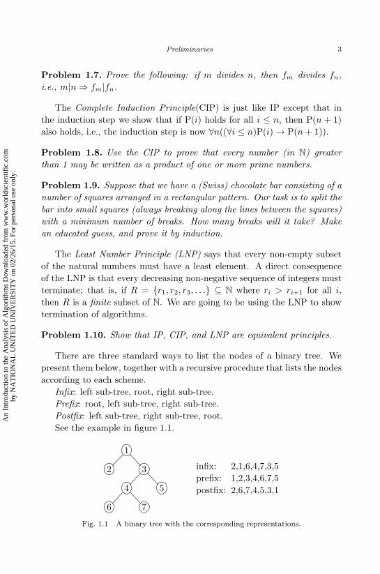
There are three standard ways to list the nodes of a binary tree. We
present them below, together with a recursive procedure that lists the nodes
according to each scheme.
Infix: left sub-tree, root, right sub-tree.
Prefix: root, left sub-tree, right sub-tree.
Postfix: left sub-tree, right sub-tree, root.
See the example in figure 1.1.
1
2 3
4 5
6 7
infix: 2,1,6,4,7,3,5
prefix: 1,2,3,4,6,7,5
postfix: 2,6,7,4,5,3,1
Fig. 1.1 A binary tree with the corresponding representations.
An
Intr
oduc
tion
to th
e A
naly
sis
of A
lgor
ithm
s D
ownl
oade
d fr
om w
ww
.wor
ldsc
ient
ific
.com
by N
AT
ION
AL
UN
ITE
D U
NIV
ER
SIT
Y o
n 02
/26/
15. F
or p
erso
nal u
se o
nly.

April 3, 2012 10:24 World Scientific Book - 9in x 6in soltys˙alg
4 An Introduction to the Analysis of Algorithms
Note that some authors use a different name for infix, prefix, and postfix;
they call it inorder, preorder, and postorder, respectively.
Problem 1.11. Show that given any two representations we can obtain
from them the third one, or, put another way, from any two representations
we can reconstruct the tree. Show, using induction, that your reconstruction
is correct. Then show that having just one representation is not enough.
Problem 1.12. Write a Python program that takes as input two of the
three descriptions, and outputs the third. One way to present the input is
as a text file, consisting of two rows, for example
infix: 2,1,6,4,7,3,5
postfix: 2,6,7,4,5,3,1
and the corresponding output would be: prefix: 1,2,3,4,6,7,5. Note
that each row of the input has to specify the “scheme” of the description.
1.2 Invariance
The Invariance Technique (IT) is a method for proving assertions about
the outcomes of procedures. The IT identifies some property that remains
true throughout the execution of a procedure. Then, once the procedure
terminates, we use this property to prove assertions about the output.
As an example, consider an 8 × 8 board from which two squares from
opposing corners have been removed (see figure 1.2). The area of the board
is 64−2 = 62 squares. Now suppose that we have 31 dominoes of size 1×2.
We want to show that the board cannot be covered by them.
Fig. 1.2 An 8× 8 board.
An
Intr
oduc
tion
to th
e A
naly
sis
of A
lgor
ithm
s D
ownl
oade
d fr
om w
ww
.wor
ldsc
ient
ific
.com
by N
AT
ION
AL
UN
ITE
D U
NIV
ER
SIT
Y o
n 02
/26/
15. F
or p
erso
nal u
se o
nly.

April 3, 2012 10:24 World Scientific Book - 9in x 6in soltys˙alg
Preliminaries 5
Verifying this by brute force (that is, examining all possible coverings)
is an extremely laborious job. However, using IT we argue as follows: color
the squares as a chess board. Each domino, covering two adjacent squares,
covers 1 white and 1 black square, and, hence, each placement covers as
many white squares as it covers black squares. Note that the number of
white squares and the number of black squares differ by 2—opposite corners
lying on the same diagonal have the same color—and, hence, no placement
of dominoes yields a cover; done!
More formally, we place the dominoes one by one on the board, any way
we want. The invariant is that after placing each new domino, the number
of covered white squares is the same as the number of covered black squares.
We prove that this is an invariant by induction on the number of placed
dominoes. The basis case is when zero dominoes have been placed (so zero
black and zero white squares are covered). In the induction step, we add
one more domino which, no matter how we place it, covers one white and
one black square, thus maintaining the property. At the end, when we
are done placing dominoes, we would have to have as many white squares
as black squares covered, which is not possible due to the nature of the
coloring of the board (i.e., the number of black and whites squares is not
the same). Note that this argument extends easily to the n× n board.
Problem 1.13. Let n be an odd number, and suppose that we have the set
{1, 2, . . . , 2n}. We pick any two numbers a, b in the set, delete them from
the set, and replace them with |a−b|. Continue repeating this until just one
number remains in the set; show that this remaining number must be odd.
The next three problems have the common theme of social gatherings.
We always assume that relations of likes and dislikes, of being an enemy or
a friend, are reflexive relations: that is, if a likes b, then b also likes a, etc.
See appendix B for background on relations—reflexive relations are defined
on page 157.
Problem 1.14. At a country club, each member dislikes at most three other
members. There are two tennis courts; show that each member can be
assigned to one of the two courts in such a way that at most one person
they dislike is also playing on the same court.
We use the vocabulary of “country clubs” and “tennis courts,” but it is
clear that Problem 1.14 is a typical situation that one might encounter in
computer science: for example, a multi-threaded program which is run on
An
Intr
oduc
tion
to th
e A
naly
sis
of A
lgor
ithm
s D
ownl
oade
d fr
om w
ww
.wor
ldsc
ient
ific
.com
by N
AT
ION
AL
UN
ITE
D U
NIV
ER
SIT
Y o
n 02
/26/
15. F
or p
erso
nal u
se o
nly.

April 3, 2012 10:24 World Scientific Book - 9in x 6in soltys˙alg
6 An Introduction to the Analysis of Algorithms
two processors, where a pair of threads are taken to be “enemies” when they
use many of the same resources. Threads that require the same resources
ought to be scheduled on different processors—as much as possible. In a
sense, these seemingly innocent problems are parables of computer science.
Problem 1.15. You are hosting a dinner party where 2n people are going to
be sitting at a round table. As it happens in any social clique, animosities
are rife, but you know that everyone sitting at the table dislikes at most
(n−1) people; show that you can make sitting arrangements so that nobody
sits next to someone they dislike.
Problem 1.16. Handshakes are exchanged at a meeting. We call a person
an odd person if he has exchanged an odd number of handshakes. Show
that, at any moment, there is an even number of odd persons.
1.3 Correctness of algorithms
How can we prove that an algorithm is correct1? We make two assertions,
called the pre-condition and the post-condition; by correctness we mean that
whenever the pre-condition holds before the algorithm executes, the post-
condition will hold after it executes. By termination we mean that whenever
the pre-condition holds, the algorithm will stop running after finitely many
steps. Correctness without termination is called partial correctness, and
correctness per se is partial correctness with termination.
These concepts can be made more precise: let A be an algorithm, and
let IA be the set of all well-formed inputs for A; the idea is that if I ∈ IAthen it “makes sense” to give I as an input to A. The concept of a “well-
formed” input can also be made precise, but it is enough to rely on our
intuitive understanding—for example, an algorithm that takes a pair of
integers as input will not be “fed” a matrix. Let O = A(I) be the output
of A on I, if it exists. Let αA be a pre-condition and βA a post-condition
of A; if I satisfies the pre-condition we write αA(I) and if O satisfies the
post-condition we write βA(O). Then, partial correctness of A with respect
to pre-condition αA and post-condition βA can be stated as:
(∀I ∈ IA)[(αA(I) ∧ ∃O(O = A(I)))→ βA(A(I))], (1.3)
1A wonderful introduction to this topic can be found in [Harel (1987)], in chapter 5,
“The correctness of algorithms, or getting it done right.”
An
Intr
oduc
tion
to th
e A
naly
sis
of A
lgor
ithm
s D
ownl
oade
d fr
om w
ww
.wor
ldsc
ient
ific
.com
by N
AT
ION
AL
UN
ITE
D U
NIV
ER
SIT
Y o
n 02
/26/
15. F
or p
erso
nal u
se o
nly.

April 3, 2012 10:24 World Scientific Book - 9in x 6in soltys˙alg
Preliminaries 7
which in words states the following: for any well formed input I, if I satisfies
the pre-condition and A(I) produces an output, i.e., terminates, which is
stated as ∃O(O = A(I)), then this output satisfies the post-condition.
Full correctness is (1.3) together with the assertion that for all I ∈ IA,
A(I) terminates (and hence there exists an O such that O = A(I)).
A fundamental notion in the analysis of algorithms is that of a loop
invariant; it is an assertion that stays true after each execution of a “while”
(or “for”) loop. Coming up with the right assertion, and proving it, is a
creative endeavor. If the algorithm terminates, the loop invariant is an
assertion that helps to prove the implication αA(I)→ βA(A(I)).
Once the loop invariant has been shown to hold, it is used for proving
partial correctness of the algorithm. So the criterion for selecting a loop
invariant is that it helps in proving the post-condition. In general many
different loop invariants (and for that matter pre and post-conditions) may
yield a desirable proof of correctness; the art of the analysis of algorithms
consists in selecting them judiciously. We usually need induction to prove
that a chosen loop invariant holds after each iteration of a loop, and usually
we also need the pre-condition as an assumption in this proof.
An implicit pre-condition of all the algorithms in this section is that the
numbers are in Z = {. . . ,−2,−1, 0, 1, 2, . . .}.
1.3.1 Division algorithm
We analyze the algorithm for integer division, algorithm 1.1. Note that the
q and r returned by the division algorithm are usually denoted as div(x, y)
(the quotient) and rem(x, y) (the remainder), respectively.
Algorithm 1.1 Division
Pre-condition: x ≥ 0 ∧ y > 0
1: q ← 0
2: r ← x
3: while y ≤ r do
4: r ← r − y5: q ← q + 1
6: end while
7: return q, r
Post-condition: x = (q · y) + r ∧ 0 ≤ r < y
An
Intr
oduc
tion
to th
e A
naly
sis
of A
lgor
ithm
s D
ownl
oade
d fr
om w
ww
.wor
ldsc
ient
ific
.com
by N
AT
ION
AL
UN
ITE
D U
NIV
ER
SIT
Y o
n 02
/26/
15. F
or p
erso
nal u
se o
nly.
April 3, 2012 10:24 World Scientific Book - 9in x 6in soltys˙alg
8 An Introduction to the Analysis of Algorithms
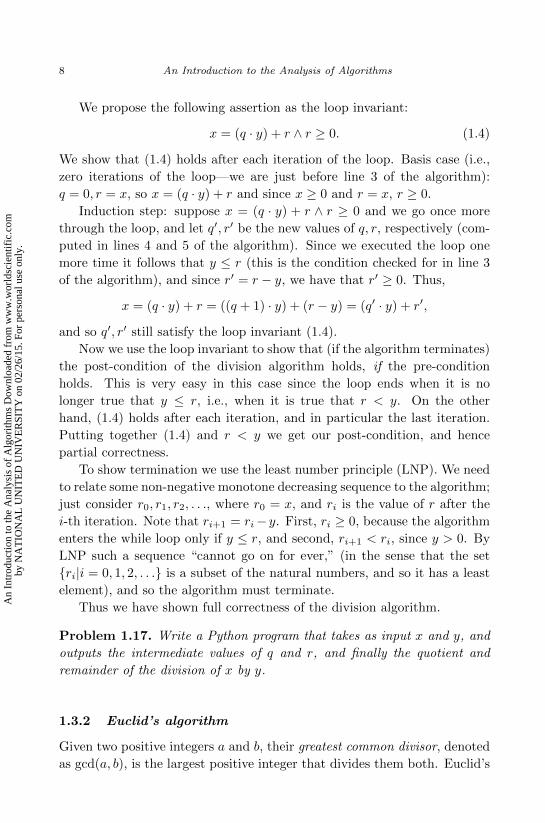
We propose the following assertion as the loop invariant:
x = (q · y) + r ∧ r ≥ 0. (1.4)
We show that (1.4) holds after each iteration of the loop. Basis case (i.e.,
zero iterations of the loop—we are just before line 3 of the algorithm):
q = 0, r = x, so x = (q · y) + r and since x ≥ 0 and r = x, r ≥ 0.
Induction step: suppose x = (q · y) + r ∧ r ≥ 0 and we go once more
through the loop, and let q′, r′ be the new values of q, r, respectively (com-
puted in lines 4 and 5 of the algorithm). Since we executed the loop one
more time it follows that y ≤ r (this is the condition checked for in line 3
of the algorithm), and since r′ = r − y, we have that r′ ≥ 0. Thus,
x = (q · y) + r = ((q + 1) · y) + (r − y) = (q′ · y) + r′,
and so q′, r′ still satisfy the loop invariant (1.4).
Now we use the loop invariant to show that (if the algorithm terminates)
the post-condition of the division algorithm holds, if the pre-condition
holds. This is very easy in this case since the loop ends when it is no
longer true that y ≤ r, i.e., when it is true that r < y. On the other
hand, (1.4) holds after each iteration, and in particular the last iteration.
Putting together (1.4) and r < y we get our post-condition, and hence
partial correctness.
To show termination we use the least number principle (LNP). We need
to relate some non-negative monotone decreasing sequence to the algorithm;
just consider r0, r1, r2, . . ., where r0 = x, and ri is the value of r after the
i-th iteration. Note that ri+1 = ri−y. First, ri ≥ 0, because the algorithm
enters the while loop only if y ≤ r, and second, ri+1 < ri, since y > 0. By
LNP such a sequence “cannot go on for ever,” (in the sense that the set
{ri|i = 0, 1, 2, . . .} is a subset of the natural numbers, and so it has a least
element), and so the algorithm must terminate.
Thus we have shown full correctness of the division algorithm.
Problem 1.17. Write a Python program that takes as input x and y, and
outputs the intermediate values of q and r, and finally the quotient and
remainder of the division of x by y.
1.3.2 Euclid’s algorithm
Given two positive integers a and b, their greatest common divisor, denoted
as gcd(a, b), is the largest positive integer that divides them both. Euclid’s
An
Intr
oduc
tion
to th
e A
naly
sis
of A
lgor
ithm
s D
ownl
oade
d fr
om w
ww
.wor
ldsc
ient
ific
.com
by N
AT
ION
AL
UN
ITE
D U
NIV
ER
SIT
Y o
n 02
/26/
15. F
or p
erso
nal u
se o
nly.

April 3, 2012 10:24 World Scientific Book - 9in x 6in soltys˙alg
Preliminaries 9
algorithm, presented as algorithm 1.2, is a procedure for finding the greatest
common divisor of two numbers. It is one of the oldest know algorithms—
it appeared in Euclid’s Elements (Book 7, Propositions 1 and 2) around
300 BC.
Algorithm 1.2 Euclid
Pre-condition: a > 0 ∧ b > 0
1: m← a ; n← b ; r ← rem(m,n)
2: while (r > 0) do
3: m← n ; n← r ; r ← rem(m,n)
4: end while
5: return n
Post-condition: n = gcd(a, b)
Note that to compute rem(n,m) in lines 1 and 3 of Euclid’s algorithm
we need to use algorithm 1.1 (the division algorithm) as a subroutine; this
is a typical “composition” of algorithms. Also note that lines 1 and 3 are
executed from left to right, so in particular in line 3 we first do m ← n,
then n← r and finally r ← rem(m,n). This is important for the algorithm
to work correctly.
To prove the correctness of Euclid’s algorithm we are going to show that
after each iteration of the while loop the following assertion holds:
m > 0, n > 0 and gcd(m,n) = gcd(a, b), (1.5)
that is, (1.5) is our loop invariant. We prove this by induction on the
number of iterations. Basis case: after zero iterations (i.e., just before the
while loop starts—so after executing line 1 and before executing line 2) we
have that m = a > 0 and n = b > 0, so (1.5) holds trivially. Note that
a > 0 and b > 0 by the pre-condition.
For the induction step, suppose m,n > 0 and gcd(a, b) = gcd(m,n),
and we go through the loop one more time, yielding m′, n′. We want to
show that gcd(m,n) = gcd(m′, n′). Note that from line 3 of the algorithm
we see that m′ = n, n′ = r = rem(m,n), so in particular m′ = n > 0 and
n′ = r = rem(m,n) > 0 since if r = rem(m,n) were zero, the loop would
have terminated (and we are assuming that we are going through the loop
one more time). So it is enough to prove the assertion in Problem 1.18.
An
Intr
oduc
tion
to th
e A
naly
sis
of A
lgor
ithm
s D
ownl
oade
d fr
om w
ww
.wor
ldsc
ient
ific
.com
by N
AT
ION
AL
UN
ITE
D U
NIV
ER
SIT
Y o
n 02
/26/
15. F
or p
erso
nal u
se o
nly.

April 3, 2012 10:24 World Scientific Book - 9in x 6in soltys˙alg
10 An Introduction to the Analysis of Algorithms
Problem 1.18. Show that for all m,n > 0, gcd(m,n) = gcd(n, rem(m,n)).
Now the correctness of Euclid’s algorithm follows from (1.5), since the
algorithm stops when r = rem(m,n) = 0, som = q·n, and so gcd(m,n) = n.
Problem 1.19. Show that Euclid’s algorithm terminates.
Problem 1.20. Do you have any ideas how to speed-up Euclid’s algorithm?
Problem 1.21. Modify Euclid’s algorithm so that given integers m,n as
input, it outputs integers a, b such that am + bn = g = gcd(m,n). This is
called the extended Euclid’s algorithm.
(a) Use the LNP to show that if g = gcd(m,n), then there exist a, b such
that am+ bn = g.
(b) Design Euclid’s extended algorithm, and prove its correctness.
(c) The usual Euclid’s extended algorithm has a running time polynomial
in min{m,n}; show that this is the running time of your algorithm, or
modify your algorithm so that it runs in this time.
Problem 1.22. Write a Python program that implements Euclid’s extended
algorithm. Then perform the following experiment: run it on a random
selection of inputs of a given size, for sizes bounded by some parameter N ;
compute the average number of steps of the algorithm for each input size
n ≤ N , and use gnuplot2 to plot the result. What does f(n)—which is
the “average number of steps” of Euclid’s extended algorithm on input size
n—look like? Note that size is not the same as value; inputs of size n are
inputs with a binary representation of n bits.
1.3.3 Palindromes algorithm
Algorithm 1.3 tests strings for palindromes, which are strings that read the
same backwards as forwards, for example, madamimadam or racecar.
Let the loop invariant be: after the k-th iteration, i = k + 1 and for
all j such that 1 ≤ j ≤ k, A[j] = A[n − j + 1]. We prove that the loop
invariant holds by induction on k. Basis case: before any iterations take
place, i.e., after zero iterations, there are no j’s such that 1 ≤ j ≤ 0, so the
2Gnuplot is a command-line driven graphing utility with versions for most platforms.If you do not already have it, you can download it from http://www.gnuplot.info . If
you prefer, you can use any other plotting utility.
An
Intr
oduc
tion
to th
e A
naly
sis
of A
lgor
ithm
s D
ownl
oade
d fr
om w
ww
.wor
ldsc
ient
ific
.com
by N
AT
ION
AL
UN
ITE
D U
NIV
ER
SIT
Y o
n 02
/26/
15. F
or p
erso
nal u
se o
nly.

April 3, 2012 10:24 World Scientific Book - 9in x 6in soltys˙alg
Preliminaries 11
Algorithm 1.3 Palindromes
Pre-condition: n ≥ 1 ∧A[1 . . . n] is a character array
1: i← 1
2: while (i ≤ bn2 c) do
3: if (A[i] 6= A[n− i+ 1]) then
4: return F
5: i← i+ 1
6: end if
7: end while
8: return T
Post-condition: return T iff A is a palindrome
second part of the loop invariant is (vacuously) true. The first part of the
loop invariant holds since i is initially set to 1.
Induction step: we know that after k iterations, A[j] = A[n−j+1] for all
1 ≤ j ≤ k; after one more iteration we know that A[k+1] = A[n−(k+1)+1],
so the statement follows for all 1 ≤ j ≤ k+1. This proves the loop invariant.
Problem 1.23. Using the loop invariant argue the partial correctness of
the palindromes algorithm. Show that the algorithm for palindromes always
terminates.
In is easy to manipulate strings in Python; a segment of a string is
called a slice. Consider the word palindrome; if we set the variables s to
this word,
s = ’palindrome’
then we can access different slices as follows:
print s[0:5] palin
print s[5:10] drome
print s[5:] drome
print s[2:8:2] lnr
where the notation [i:j] means the segment of the string starting from the
i-th character (and we always start counting at zero!), to the j-th character,
including the first but excluding the last. The notation [i:] means from
the i-th character, all the way to the end, and [i:j:k] means starting from
the i-th character to the j-th (again, not including the j-th itself), taking
every k-th character.
An
Intr
oduc
tion
to th
e A
naly
sis
of A
lgor
ithm
s D
ownl
oade
d fr
om w
ww
.wor
ldsc
ient
ific
.com
by N
AT
ION
AL
UN
ITE
D U
NIV
ER
SIT
Y o
n 02
/26/
15. F
or p
erso
nal u
se o
nly.

April 3, 2012 10:24 World Scientific Book - 9in x 6in soltys˙alg
12 An Introduction to the Analysis of Algorithms
One way to understand the string delimiters is to write the indices “in
between” the numbers, as well as at the beginning and at the end. For
example
0p1a2l3i4n5d6r7o8m9e10
and to notice that a slice [i:j] contains all the symbols between index i
and index j.
Problem 1.24. Using Python’s inbuilt facilities for manipulating slices of
strings, write a succinct program that checks whether a given string is a
palindrome.
1.3.4 Further examples
Problem 1.25. Give an algorithm which on the input “a positive integer
n,” outputs “yes” if n = 2k (i.e., n is a power of 2), and “no” otherwise.
Prove that your algorithm is correct.
Problem 1.26. What does algorithm 1.4 compute? Prove your claim.
Algorithm 1.4 Problem 1.26
1: x← m ; y ← n ; z ← 0
2: while (x 6= 0) do
3: if (rem(x, 2) = 1) then
4: z ← z + y
5: end if
6: x← div(x, 2)
7: y ← y · 28: end while
9: return z
Problem 1.27. What does algorithm 1.5 compute? Assume that a, b are
positive integers (i.e., assume that the pre-condition is that a, b > 0). For
which starting a, b does this algorithm terminate? In how many steps does
it terminate, if it does terminate?
The following two problems require some linear algebra3. We say that
a set of vectors {v1, v2, . . . , vn} is linearly independent if∑ni=1 civi = 0
implies that ci = 0 for all i, and that they span a vector space V ⊆ Rn3A great and accessible introduction to linear algebra can be found in [Halmos (1995)].
An
Intr
oduc
tion
to th
e A
naly
sis
of A
lgor
ithm
s D
ownl
oade
d fr
om w
ww
.wor
ldsc
ient
ific
.com
by N
AT
ION
AL
UN
ITE
D U
NIV
ER
SIT
Y o
n 02
/26/
15. F
or p
erso
nal u
se o
nly.

April 3, 2012 10:24 World Scientific Book - 9in x 6in soltys˙alg
Preliminaries 13
Algorithm 1.5 Problem 1.27
1: while (a > 0) do
2: if (a < b) then
3: (a, b)← (2a, b− a)
4: else
5: (a, b)← (a− b, 2b)6: end if
7: end while
if whenever v ∈ V , then there exist ci ∈ R such that v =∑ni=1 civi. We
denote this as V = span{v1, v2, . . . , vn}. A set of vectors {v1, v2, . . . , vn}in Rn is a basis for a vector space V ⊆ Rn if they are linearly independent
and span V . Let x · y denote the dot-product of two vectors, defined as
x · y = (x1, x2, . . . , xn) · (y1, y2, . . . , yn) =∑ni=1 xiyi, and the norm of a
vector x is defined as ‖x‖ =√x · x. Two vectors x, y are orthogonal if
x · y = 0.
Problem 1.28. Let V ⊆ Rn be a vector space, and {v1, v2, . . . , vn} its
basis. Consider algorithm 1.6 and show that it produces an orthogonal basis
Algorithm 1.6 Gram-Schmidt
Pre-condition: {v1, . . . , vn} a basis for Rn1: v∗1 ←− v12: for i = 2, 3, . . . , n do
3: for j = 1, 2, . . . , (i− 1) do
4: µij ←− (vi · v∗j )/‖v∗j ‖25: end for
6: v∗i ←− vi −∑i−1j=1 µijv
∗j
7: end for
Post-condition: {v∗1 , . . . , v∗n} an orthogonal basis for Rn
{v∗1 , v∗2 , . . . , v∗n} for the vector space V . In other words, show that v∗i ·v∗j = 0
when i 6= j, and that span{v1, v2, . . . , vn} = span{v∗1 , v∗2 , . . . , v∗n}. Justify
why in line 4 of the algorithm we never divide by zero.
Problem 1.29. Implement the Gram-Schmidt algorithm (algorithm 1.6)
in Python, but with the following twist: instead of computing over R, the
real numbers, compute over Z2, the field of two elements, where addition
and multiplication are defined as follows:
An
Intr
oduc
tion
to th
e A
naly
sis
of A
lgor
ithm
s D
ownl
oade
d fr
om w
ww
.wor
ldsc
ient
ific
.com
by N
AT
ION
AL
UN
ITE
D U
NIV
ER
SIT
Y o
n 02
/26/
15. F
or p
erso
nal u
se o
nly.
April 3, 2012 10:24 World Scientific Book - 9in x 6in soltys˙alg
14 An Introduction to the Analysis of Algorithms
+ 0 1
0 0 1
1 1 0
· 0 1
0 0 0
1 0 1In fact, this “twist” makes the implementation much easier, as you do not
have to deal with the precision issues involved in implementing division
operations over the field of real numbers.
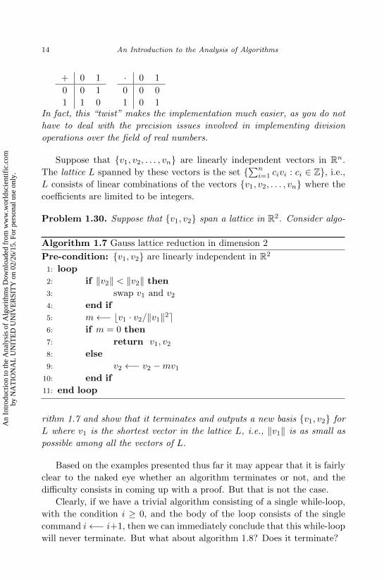
Suppose that {v1, v2, . . . , vn} are linearly independent vectors in Rn.
The lattice L spanned by these vectors is the set {∑ni=1 civi : ci ∈ Z}, i.e.,
L consists of linear combinations of the vectors {v1, v2, . . . , vn} where the
coefficients are limited to be integers.
Problem 1.30. Suppose that {v1, v2} span a lattice in R2. Consider algo-
Algorithm 1.7 Gauss lattice reduction in dimension 2
Pre-condition: {v1, v2} are linearly independent in R2
1: loop
2: if ‖v2‖ < ‖v2‖ then
3: swap v1 and v24: end if
5: m←− bv1 · v2/‖v1‖2e6: if m = 0 then
7: return v1, v28: else
9: v2 ←− v2 −mv110: end if
11: end loop
rithm 1.7 and show that it terminates and outputs a new basis {v1, v2} for
L where v1 is the shortest vector in the lattice L, i.e., ‖v1‖ is as small as
possible among all the vectors of L.
Based on the examples presented thus far it may appear that it is fairly
clear to the naked eye whether an algorithm terminates or not, and the
difficulty consists in coming up with a proof. But that is not the case.
Clearly, if we have a trivial algorithm consisting of a single while-loop,
with the condition i ≥ 0, and the body of the loop consists of the single
command i←− i+1, then we can immediately conclude that this while-loop
will never terminate. But what about algorithm 1.8? Does it terminate?
An
Intr
oduc
tion
to th
e A
naly
sis
of A
lgor
ithm
s D
ownl
oade
d fr
om w
ww
.wor
ldsc
ient
ific
.com
by N
AT
ION
AL
UN
ITE
D U
NIV
ER
SIT
Y o
n 02
/26/
15. F
or p
erso
nal u
se o
nly.

April 3, 2012 10:24 World Scientific Book - 9in x 6in soltys˙alg
Preliminaries 15
Algorithm 1.8 Ulam’s algorithm
Pre-condition: a > 0
x←− awhile last three values of x not 4, 2, 1 do
if x is even then
x←− x/2else
x←− 3x+ 1
end if
end while
For example, if a = 22, then one can check that x takes on the following
values: 22, 11, 34, 17, 52, 26, 13, 40, 20, 10, 5, 16, 8,4,2,1, and algorithm 1.8
terminates.
It is conjectured that regardless of the initial value of a, as long as a
is a positive integer, algorithm 1.8 terminates. This conjecture is known
as “Ulam’s problem,”4 No one has been able to prove that algorithm 1.8
terminates, and in fact proving termination would involve solving a difficult
open mathematical problem.
Problem 1.31. Write a Python program that takes a as input and com-
putes and displays all the values of Ulam’s problem until it sees 4, 2, 1 at
which point it stops. You have just written a program for which there is no
proof of termination.
1.3.5 Recursion and fixed points
So far we have proved the correctness of while-loops and for-loops, but there
is another way of “looping” using recursive procedures, i.e., algorithms that
“call themselves.” We are going to see examples of such algorithms in the
chapter on the divide and conquer method.
There is a robust theory of correctness of recursive algorithms based on
fixed point theory, and in particular on Kleene’s theorem (see appendix B,
theorem B.39). We briefly illustrate this approach with an example. We
are going to be using partial orders; all the necessary background can be
found in appendix B, in section B.3. Consider the recursive algorithm 1.9.
4It is also called “Collatz Conjecture,” “Syracuse Problem,” “Kakutani’s Problem,”or “Hasse’s Algorithm.” While it is true that a rose by any other name would smell
just as sweet, the preponderance of names shows that the conjecture is a very alluring
An
Intr
oduc
tion
to th
e A
naly
sis
of A
lgor
ithm
s D
ownl
oade
d fr
om w
ww
.wor
ldsc
ient
ific
.com
by N
AT
ION
AL
UN
ITE
D U
NIV
ER
SIT
Y o
n 02
/26/
15. F
or p
erso
nal u
se o
nly.
April 3, 2012 10:24 World Scientific Book - 9in x 6in soltys˙alg
16 An Introduction to the Analysis of Algorithms
Algorithm 1.9 F (x, y)
1: if x = y then
2: return y + 1
3: else
4: F (x, F (x− 1, y + 1))
5: end if
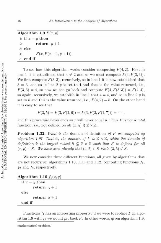
To see how this algorithm works consider computing F (4, 2). First in
line 1 it is established that 4 6= 2 and so we must compute F (4, F (3, 3)).
We first compute F (3, 3), recursively, so in line 1 it is now established that
3 = 3, and so in line 2 y is set to 4 and that is the value returned, i.e.,
F (3, 3) = 4, so now we can go back and compute F (4, F (3, 3)) = F (4, 4),
so again, recursively, we establish in line 1 that 4 = 4, and so in line 2 y is
set to 5 and this is the value returned, i.e., F (4, 2) = 5. On the other hand
it is easy to see that
F (3, 5) = F (3, F (2, 6)) = F (3, F (2, F (1, 7))) = · · · ,
and this procedure never ends as x will never equal y. Thus F is not a total
function, i.e., not defined on all (x, y) ∈ Z× Z.
Problem 1.32. What is the domain of definition of F as computed by
algorithm 1.9? That is, the domain of F is Z × Z, while the domain of
definition is the largest subset S ⊆ Z × Z such that F is defined for all
(x, y) ∈ S. We have seen already that (4, 2) ∈ S while (3, 5) 6∈ S.
We now consider three different functions, all given by algorithms that
are not recursive: algorithms 1.10, 1.11 and 1.12, computing functions f1,
f2 and f3, respectively.
Algorithm 1.10 f1(x, y)
if x = y then
return y + 1
else
return x+ 1
end if
Functions f1 has an interesting property: if we were to replace F in algo-
rithm 1.9 with f1 we would get back F . In other words, given algorithm 1.9,
mathematical problem.
An
Intr
oduc
tion
to th
e A
naly
sis
of A
lgor
ithm
s D
ownl
oade
d fr
om w
ww
.wor
ldsc
ient
ific
.com
by N
AT
ION
AL
UN
ITE
D U
NIV
ER
SIT
Y o
n 02
/26/
15. F
or p
erso
nal u
se o
nly.

April 3, 2012 10:24 World Scientific Book - 9in x 6in soltys˙alg
Preliminaries 17
if we were to replace line 4 with f1(x, f1(x−1, y+1)), and compute f1 with
the (non-recursive) algorithm 1.10 for f1, then algorithm 1.9 thus modified
would now be computing F (x, y). Therefore, we say that the functions f1is a fixed point of the recursive algorithm 1.9.
For example, recall the we have already shown that F (4, 2) = 5, using
the recursive algorithm 1.9 for computing F . Replace line 4 in algorithm 1.9
with f1(x, f1(x − 1, y + 1)) and compute F (4, 2) anew; since 4 6= 2 we go
directly to line 4 where we compute f1(4, f1(3, 3)) = f1(4, 4) = 5. Notice
that this last computation was not recursive, as we computed f1 directly
with algorithm 1.10, and that we have obtained the same value.
Consider now f2, f3, computed by algorithms 1.11, 1.12, respectively.
Algorithm 1.11 f2(x, y)
if x ≥ y then
return x+ 1
else
return y − 1
end if
Algorithm 1.12 f3(x, y)
if x ≥ y ∧ (x− y is even) then
return x+ 1
end if
Notice that in algorithm 1.12, if it is not the case that x ≥ y and x− yis even, then the output is undefined. Thus f3 is a partial function, and if
x < y or x− y is odd, then (x, y) is not in its domain of definition.
Problem 1.33. Prove that f1, f2, f3 are all fixed points of algorithm 1.9.
The function f3 has one additional property. For every pair of integers
x, y such that f3(x, y) is defined, that is x ≥ y and x−y is even, both f1(x, y)
and f2(x, y) are also defined and have the same value as f3(x, y). We say
that f3 is less defined than or equal to f1 and f2, and write f3 v f1 and
f3 v f2; that is, we have defined (informally) a partial order on functions
f : Z× Z −→ Z× Z.
Problem 1.34. Show that f3 v f1 and f3 v f2. Recall the notion of
a domain of definition introduced in problem 1.32. Let S1, S2, S3 be the
An
Intr
oduc
tion
to th
e A
naly
sis
of A
lgor
ithm
s D
ownl
oade
d fr
om w
ww
.wor
ldsc
ient
ific
.com
by N
AT
ION
AL
UN
ITE
D U
NIV
ER
SIT
Y o
n 02
/26/
15. F
or p
erso
nal u
se o
nly.

April 3, 2012 10:24 World Scientific Book - 9in x 6in soltys˙alg
18 An Introduction to the Analysis of Algorithms
domains of definition of f1, f2, f3, respectively. You must show that S3 ⊆ S1
and S3 ⊆ S2.
It can be shown that f3 has this property, not only with respect to f1and f2, but also with respect to all fixed points of algorithm 1.9. Moreover,
f3(x, y) is the only function having this property, and therefore f3 is said to
be the least (defined) fixed point of algorithm 1.9. It is an important appli-
cation of Kleene’s theorem (theorem B.39) that every recursive algorithm
has a unique fixed point.
1.3.6 Formal verification
The proofs of correctness we have been giving thus far are considered to be
“informal” mathematical proofs. There is nothing wrong with an informal
proof, and in many cases such a proof is all that is necessary to convince
oneself of the validity of a small “code snippet.” However, there are many
circumstances where extensive formal code validation is necessary; in that
case, instead of an informal paper-and-pencil type of argument, we often
employ computer assisted software verification. For example, the US Food
and Drug Administration requires software certification in cases where med-
ical devices are dependent on software for their effective and safe operation.
When formal verification is required everything has to be stated explicitly,
in a formal language, and proven painstakingly line by line. In this section
we give an example of such a procedure.
Let {α}P{β} mean that if formula α is true before execution of P , P
is executed and terminates, then formula β will be true, i.e., α, β, are the
precondition and postcondition of the program P , respectively. They are
usually given as formulas in some formal theory, such as first order logic
over some language L. We assume that the language is Peano Arithmetic;
see Appendix C.
Using a finite set of rules for program verification, we want to show that
{α}P{β} holds, and conclude that the program is correct with respect to
the specification α, β. As our example is small, we are going to use a limited
set of rules for program verification, given in figure 1.3
The “If” rule is saying the following: suppose that it is the case that
{α ∧ β}P1{γ} and {α ∧ ¬β}P2{γ}. This means that P1 is (partially) cor-
rect with respect to precondition α ∧ β and postcondition γ, while P2 is
(partially) correct with respect to precondition α ∧ ¬β and postcondition
γ. Then the program “if β then P1 else P2” is (partially) correct with
An
Intr
oduc
tion
to th
e A
naly
sis
of A
lgor
ithm
s D
ownl
oade
d fr
om w
ww
.wor
ldsc
ient
ific
.com
by N
AT
ION
AL
UN
ITE
D U
NIV
ER
SIT
Y o
n 02
/26/
15. F
or p
erso
nal u
se o
nly.

April 3, 2012 10:24 World Scientific Book - 9in x 6in soltys˙alg
Preliminaries 19
Consequence left and right
{α}P{β} (β → γ)
{α}P{γ}(γ → α) {α}P{β}
{γ}P{β}Composition and assignment
{α}P1{β} {β}P2{γ}{α}P1P2{γ}
x := t
{α(t)}x := t{α(x)}If
{α ∧ β}P1{γ} {α ∧ ¬β}P2{γ}{α} if β then P1 else P2 {γ}
While
{α ∧ β}P{α}{α} while β do P {α ∧ ¬β}
Fig. 1.3 A small set of rules for program verification.
respect to precondition α and postcondition γ because if α holds before it
executes, then either β or ¬β must be true, and so either P1 or P2 executes,
respectively, giving us γ in both cases.
The “While” rule is saying the following: suppose it is the case that
{α ∧ β}P{α}. This means that P is (partially) correct with respect to
precondition α ∧ β and postcondition α. Then the program “while β do
P” is (partially) correct with respect to precondition α and postcondition
α ∧ ¬β because if α holds before it executes, then either β holds in which
case the while-loop executes once again, with α ∧ β holding, and so α still
holds after P executes, or β is false, in which case ¬β is true and the loop
terminates with α ∧ ¬β.
As an example, we verify which computes y = A · B. Note that in
algorithm 1.13, which describes the program that computes y = A · B, we
use “=” instead of the usual “←” since we are now proving the correctness
of an actual program, rather than its representation in pseudo-code.
We want to show:
{B ≥ 0}mult(A,B){y = AB} (1.6)
Each pass through the while loop adds a to y, but a·b decreases by a because
b is decremented by 1. Let the loop invariant be: (y+(a ·b) = A ·B)∧b ≥ 0.
To save space, write tu instead of t ·u. Let t ≥ u abbreviate the LA-formula
∃x(t = u+ x), and let t ≤ u abbreviate u ≥ t.
An
Intr
oduc
tion
to th
e A
naly
sis
of A
lgor
ithm
s D
ownl
oade
d fr
om w
ww
.wor
ldsc
ient
ific
.com
by N
AT
ION
AL
UN
ITE
D U
NIV
ER
SIT
Y o
n 02
/26/
15. F
or p
erso
nal u
se o
nly.
April 3, 2012 10:24 World Scientific Book - 9in x 6in soltys˙alg
20 An Introduction to the Analysis of Algorithms
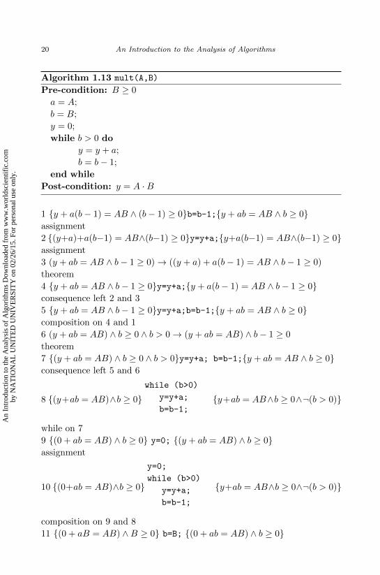
Algorithm 1.13 mult(A,B)
Pre-condition: B ≥ 0
a = A;
b = B;
y = 0;
while b > 0 do
y = y + a;
b = b− 1;
end while
Post-condition: y = A ·B
1 {y + a(b− 1) = AB ∧ (b− 1) ≥ 0}b=b-1;{y + ab = AB ∧ b ≥ 0}assignment
2 {(y+a)+a(b−1) = AB∧(b−1) ≥ 0}y=y+a;{y+a(b−1) = AB∧(b−1) ≥ 0}assignment
3 (y + ab = AB ∧ b− 1 ≥ 0)→ ((y + a) + a(b− 1) = AB ∧ b− 1 ≥ 0)
theorem
4 {y + ab = AB ∧ b− 1 ≥ 0}y=y+a;{y + a(b− 1) = AB ∧ b− 1 ≥ 0}consequence left 2 and 3
5 {y + ab = AB ∧ b− 1 ≥ 0}y=y+a;b=b-1;{y + ab = AB ∧ b ≥ 0}composition on 4 and 1
6 (y + ab = AB) ∧ b ≥ 0 ∧ b > 0→ (y + ab = AB) ∧ b− 1 ≥ 0
theorem
7 {(y + ab = AB) ∧ b ≥ 0 ∧ b > 0}y=y+a; b=b-1;{y + ab = AB ∧ b ≥ 0}consequence left 5 and 6
8 {(y+ab = AB)∧b ≥ 0}while (b>0)
y=y+a;
b=b-1;{y+ab = AB∧b ≥ 0∧¬(b > 0)}
while on 7
9 {(0 + ab = AB) ∧ b ≥ 0} y=0; {(y + ab = AB) ∧ b ≥ 0}assignment
10 {(0+ab = AB)∧b ≥ 0}
y=0;
while (b>0)
y=y+a;
b=b-1;
{y+ab = AB∧b ≥ 0∧¬(b > 0)}
composition on 9 and 8
11 {(0 + aB = AB) ∧B ≥ 0} b=B; {(0 + ab = AB) ∧ b ≥ 0}
An
Intr
oduc
tion
to th
e A
naly
sis
of A
lgor
ithm
s D
ownl
oade
d fr
om w
ww
.wor
ldsc
ient
ific
.com
by N
AT
ION
AL
UN
ITE
D U
NIV
ER
SIT
Y o
n 02
/26/
15. F
or p
erso
nal u
se o
nly.

April 3, 2012 10:24 World Scientific Book - 9in x 6in soltys˙alg
Preliminaries 21
assignment
12 {(0+aB = AB)∧B ≥ 0}
b=B;
y=0;
while (b>0)
y=y+a;
b=b-1;
{y+ab = AB∧b ≥ 0∧¬(b > 0)}
composition on 11 and 10
13 {(0 +AB = AB) ∧B ≥ 0} a=A; {(0 + aB = AB) ∧B ≥ 0}assignment
14 {(0 +AB = AB)∧B ≥ 0} mult(A,B) {y+ ab = AB ∧ b ≥ 0∧¬(b > 0)}composition on 13 and 12
15 B ≥ 0→ ((0 +AB = AB) ∧B ≥ 0)
theorem
16 (y + ab = AB ∧ b ≥ 0 ∧ ¬(b > 0))→ y = AB
theorem
17 {B ≥ 0} mult(A,B) {y + ab = AB ∧ b ≥ 0 ∧ ¬(b > 0)}consequence left on 15 and 14
18 {B ≥ 0} mult(A,B) {y = AB}consequence right on 16 and 17
Problem 1.35. The following is a project, rather than an exercise. Give
formal proofs of correctness of the division algorithm and Euclid’s algorithm
(algorithms 1.1 and 1.2). To give a complete proof you will need to use
Peano Arithmetic, which is a formalization of number theory—exactly what
is needed for these two algorithms. The details of Peano Arithmetic are
given in Appendix C.
1.4 Stable marriage
The method of “pairwise comparisons” was first described by Marquis de
Condorcet in 1785. Today rankings based on pairwise comparisons are
pervasive: scheduling of processes, online shopping and dating websites, to
name just a few. We end this chapter with an elegant application known
as the “stable marriage problem,” which has been used since the 1960s for
the college admission process and for matching interns with hospitals.
An instance of the stable marriage problem of size n consists of two
disjoint finite sets of equal size; a set of boys B = {b1, b2, . . . , bn}, and a set
An
Intr
oduc
tion
to th
e A
naly
sis
of A
lgor
ithm
s D
ownl
oade
d fr
om w
ww
.wor
ldsc
ient
ific
.com
by N
AT
ION
AL
UN
ITE
D U
NIV
ER
SIT
Y o
n 02
/26/
15. F
or p
erso
nal u
se o
nly.

April 3, 2012 10:24 World Scientific Book - 9in x 6in soltys˙alg
22 An Introduction to the Analysis of Algorithms
b
$$
g
zzpM (g) pM (b)
Fig. 1.4 A blocking pair: b and g prefer each other to their partners pM (b) and pM (g).
of girls G = {g1, g2, . . . , gn}. Let “<i” denote the ranking of boy bi; that
is, g <i g′ means that boy bi prefers g over g′. Similarly, “<j” denotes
the ranking of girl gj . Each boy bi has such a ranking (linear ordering)
<i of G which reflects his preference for the girls that he wants to marry.
Similarly each girl gj has a ranking (linear ordering) <j of B which reflects
her preference for the boys she would like to marry.
A matching (or marriage) M is a 1-1 correspondence between B and
G. We say that b and g are partners in M if they are matched in M and
write pM (b) = g and also pM (g) = b. A matching M is unstable if there
is a pair (b, g) from B × G such that b and g are not partners in M but b
prefers g to pM (b) and g prefers b to pM (g). Such a pair (b, g) is said to
block the matching M and is called a blocking pair for M (see figure 1.4).
A matching M is stable if it contains no blocking pair.
We are going to present an algorithm due to Gale and Shapley ([Gale
and Shapley (1962)]) that outputs a stable marriage for any input B,G,
regardless of the ranking.
The matching M is produced in stages Ms so that bt always has a
partner at the end of stage s, where s ≥ t. However, the partners of bt do not
get better, i.e., pMt(bt) ≤t pMt+1
(bt) ≤t · · · . On the other hand, for each
g ∈ G, if g has a partner at stage t, then g will have a partner at each stage
s ≥ t and the partners do not get worse, i.e., pMt(g) ≥t pMt+1
(g) ≥t . . ..Thus, as s increases, the partners of bt become less preferable and the
partners of g become more preferable.
At the end of stage s, assume that we have produced a matching
Ms = {(b1, g1,s), . . . , (bs, gs,s)},
where the notation gi,s means that gi,s is the partner of boy bi after the
end of stage s.
We will say that partners in Ms are engaged. The idea is that at stage
s+1, bs+1 will try to get a partner by proposing to the girls in G in his order
of preference. When bs+1 proposes to a girl gj , gj accepts his proposal if
An
Intr
oduc
tion
to th
e A
naly
sis
of A
lgor
ithm
s D
ownl
oade
d fr
om w
ww
.wor
ldsc
ient
ific
.com
by N
AT
ION
AL
UN
ITE
D U
NIV
ER
SIT
Y o
n 02
/26/
15. F
or p
erso
nal u
se o
nly.
April 3, 2012 10:24 World Scientific Book - 9in x 6in soltys˙alg
Preliminaries 23
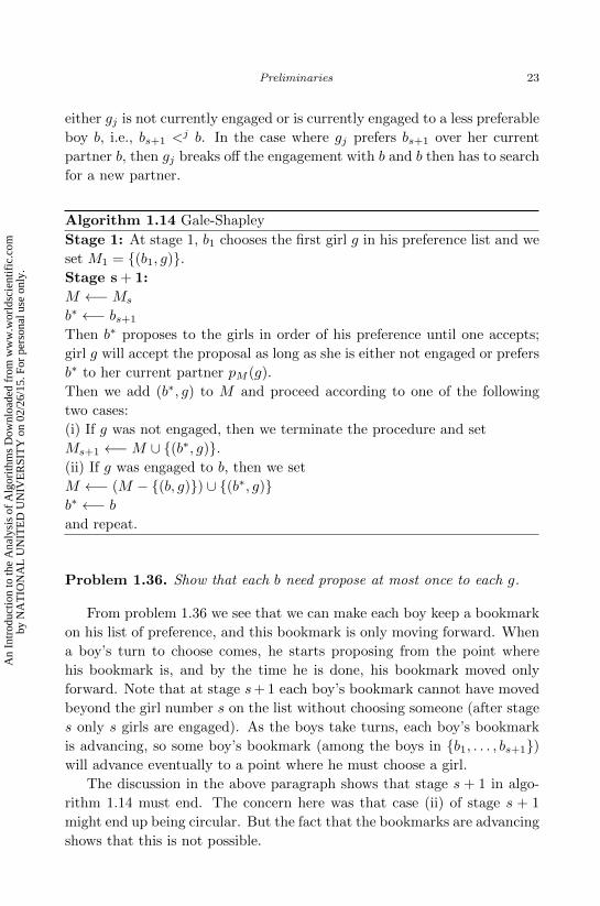
either gj is not currently engaged or is currently engaged to a less preferable
boy b, i.e., bs+1 <j b. In the case where gj prefers bs+1 over her current
partner b, then gj breaks off the engagement with b and b then has to search
for a new partner.
Algorithm 1.14 Gale-Shapley
Stage 1: At stage 1, b1 chooses the first girl g in his preference list and we
set M1 = {(b1, g)}.Stage s + 1:
M ←−Ms
b∗ ←− bs+1
Then b∗ proposes to the girls in order of his preference until one accepts;
girl g will accept the proposal as long as she is either not engaged or prefers
b∗ to her current partner pM (g).
Then we add (b∗, g) to M and proceed according to one of the following
two cases:
(i) If g was not engaged, then we terminate the procedure and set
Ms+1 ←−M ∪ {(b∗, g)}.(ii) If g was engaged to b, then we set
M ←− (M − {(b, g)}) ∪ {(b∗, g)}b∗ ←− band repeat.
Problem 1.36. Show that each b need propose at most once to each g.
From problem 1.36 we see that we can make each boy keep a bookmark
on his list of preference, and this bookmark is only moving forward. When
a boy’s turn to choose comes, he starts proposing from the point where
his bookmark is, and by the time he is done, his bookmark moved only
forward. Note that at stage s+ 1 each boy’s bookmark cannot have moved
beyond the girl number s on the list without choosing someone (after stage
s only s girls are engaged). As the boys take turns, each boy’s bookmark
is advancing, so some boy’s bookmark (among the boys in {b1, . . . , bs+1})will advance eventually to a point where he must choose a girl.
The discussion in the above paragraph shows that stage s + 1 in algo-
rithm 1.14 must end. The concern here was that case (ii) of stage s + 1
might end up being circular. But the fact that the bookmarks are advancing
shows that this is not possible.
An
Intr
oduc
tion
to th
e A
naly
sis
of A
lgor
ithm
s D
ownl
oade
d fr
om w
ww
.wor
ldsc
ient
ific
.com
by N
AT
ION
AL
UN
ITE
D U
NIV
ER
SIT
Y o
n 02
/26/
15. F
or p
erso
nal u
se o
nly.

April 3, 2012 10:24 World Scientific Book - 9in x 6in soltys˙alg
24 An Introduction to the Analysis of Algorithms
Furthermore, this gives an upper bound of (s+1)2 steps at stage (s+1)
in the procedure. This means that there are n stages, and each stage takes
O(n2) steps, and hence algorithm 1.14 takes O(n3) steps altogether. The
question, of course, is what do we mean by a step? Computers operate on
binary strings, yet here the implicit assumption is that we compare numbers
and access the lists of preferences in a single step. But the cost of these
operations is negligible when compared to our idealized running time, and
so we allow ourselves this poetic license to bound the overall running time.
Problem 1.37. Show that there is exactly one girl that was not engaged
at stage s but is engaged at stage (s + 1) and that, for each girl gj that is
engaged in Ms, gj will be engaged in Ms+1 and that pMs+1(gj) <
j pMs(gj).
(Thus, once gj becomes engaged, she will remain engaged and her partners
will only gain in preference as the stages proceed.)
Problem 1.38. Suppose that |B| = |G| = n. Show that at the end of stage
n, Mn will be a stable marriage.
We say that a matching (b, g) is feasible if there exists a stable match-
ing in which b, g are partners. We say that a matching is boy-optimal if
every boy is paired with his highest ranked feasible partner. We say that
a matching is boy-pessimal if every boy is paired with his lowest ranking
feasible partner. Similarly, we define girl-optimal/pessimal.
Problem 1.39. Show that our version of the algorithm produces a boy-
optimal and girl-pessimal stable matching.
Problem 1.40. Implement the stable marriage problem algorithm in
Python. Let the input be given as a text file containing, on each line, the
preference list for each boy and girl.
1.5 Answers to selected problems
Problem 1.2. Basis case: n = 1, then 13 = 12. For the induction step:
(1 + 2 + 3 + · · ·+ n+ (n+ 1))2
= (1 + 2 + 3 + · · ·+ n)2 + 2(1 + 2 + 3 + · · ·+ n)(n+ 1) + (n+ 1)2
An
Intr
oduc
tion
to th
e A
naly
sis
of A
lgor
ithm
s D
ownl
oade
d fr
om w
ww
.wor
ldsc
ient
ific
.com
by N
AT
ION
AL
UN
ITE
D U
NIV
ER
SIT
Y o
n 02
/26/
15. F
or p
erso
nal u
se o
nly.
April 3, 2012 10:24 World Scientific Book - 9in x 6in soltys˙alg
Preliminaries 25
and by the induction hypothesis,
= (13 + 23 + 33 + · · ·+ n3) + 2(1 + 2 + 3 + · · ·+ n)(n+ 1) + (n+ 1)2
= (13 + 23 + 33 + · · ·+ n3) + 2n(n+ 1)
2(n+ 1) + (n+ 1)2
= (13 + 23 + 33 + · · ·+ n3) + n(n+ 1)2 + (n+ 1)2
= (13 + 23 + 33 + · · ·+ n3) + (n+ 1)3
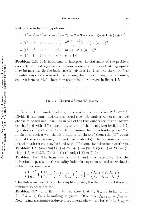
Problem 1.3. It is important to interpret the statement of the problem
correctly: when it says that one square is missing, it means that any square
may be missing. So the basis case is: given a 2 × 2 square, there are four
possible ways for a square to be missing; but in each case, the remaining
squares form an “L.” These four possibilities are drawn in figure 1.5.
Fig. 1.5 The four different “L” shapes.
Suppose the claim holds for n, and consider a square of size 2n+1×2n+1.
Divide it into four quadrants of equal size. No matter which square we
choose to be missing, it will be in one of the four quadrants; that quadrant
can be filled with “L” shapes (i.e., shapes of the form given by figure 1.5)
by induction hypothesis. As to the remaining three quadrants, put an “L”
in them in such a way that it straddles all three of them (the “L” wraps
around the center staying in those three quadrants). The remaining squares
of each quadrant can now be filled with “L” shapes by induction hypothesis.
Problem 1.4. Since ∀n(P (n)→ P (n+1))→ (∀n ≥ k)(P (n)→ P (n+1)),
then (1.2)⇒ (1.2′). On the other hand, (1.2′) 6⇒ (1.2).
Problem 1.5. The basis case is n = 1, and it is immediate. For the
induction step, assume the equality holds for exponent n, and show that it
holds for exponent n+ 1:(1 1
1 0
)n(1 1
1 0
)=
(fn+1 fnfn fn−1
)(1 1
1 0
)=
(fn+1 + fn fn+1
fn + fn−1 fn
)The right-most matrix can be simplified using the definition of Fibonacci
numbers to be as desired.
Problem 1.7. m|n iff n = km, so show that fm|fkm by induction on
k. If k = 1, there is nothing to prove. Otherwise, f(k+1)m = fkm+m.
Now, using a separate inductive argument, show that for y ≥ 1, fx+y =
An
Intr
oduc
tion
to th
e A
naly
sis
of A
lgor
ithm
s D
ownl
oade
d fr
om w
ww
.wor
ldsc
ient
ific
.com
by N
AT
ION
AL
UN
ITE
D U
NIV
ER
SIT
Y o
n 02
/26/
15. F
or p
erso
nal u
se o
nly.
April 3, 2012 10:24 World Scientific Book - 9in x 6in soltys˙alg
26 An Introduction to the Analysis of Algorithms
fyfx+1 + fy−1fx, and finish the proof. To show this last statement, let
y = 1, and note that fyfx+1 + fy−1fx = f1fx+1 + f0fx = fx+1. Assume
now that fx+y = fyfx+1 + fy−1fx holds. Consider
fx+(y+1) = f(x+y)+1 = f(x+y) + f(x+y)−1 = f(x+y) + fx+(y−1)
= (fyfx+1 + fy−1fx) + (fy−1fx+1 + fy−2fx)
= fx+1(fy + fy−1) + fx(fy−1 + fy−2)
= fx+1fy+1 + fxfy.
Problem 1.8. Note that this is almost the Fundamental Theorem of Arith-
metic; what is missing is the fact that up to reordering of primes this
representation is unique. The proof of this can be found in appendix A,
theorem A.2.
Problem 1.9. Let our assertion P(n) be: the minimal number of breaks
to break up a chocolate bar of n squares is (n − 1). Note that this says
that (n− 1) breaks are sufficient, and (n− 2) are not. Basis case: only one
square requires no breaks. Induction step: Suppose that we have m + 1
squares. No matter how we break the bar into two smaller pieces of a and
b squares each, a+ b = m+ 1.
By induction hypothesis, the “a” piece requires a − 1 breaks, and the
“b” piece requires b− 1 breaks, so together the number of breaks is
(a− 1) + (b− 1) + 1 = a+ b− 1 = m+ 1− 1 = m,
and we are done. Note that the 1 in the box comes from the initial break
to divide the chocolate bar into the “a” and the “b” pieces.
So the “boring” way of breaking up the chocolate (first into rows, and
then each row separately into pieces) is in fact optimal.
Problem 1.10. Let IP be: [P(0) ∧ (∀n)(P(n) → P(n + 1))] → (∀m)P(m)
(where n,m range over natural numbers), and let LNP: Every non-empty
subset of the natural numbers has a least element. These two principles are
equivalent, in the sense that one can be shown from the other. Indeed:
LNP⇒IP: Suppose we have [P(0) ∧ (∀n)(P(n)→ P(n+ 1))], but that
it is not the case that (∀m)P(m). Then, the set S of m’s for which P(m)
is false is non-empty. By the LNP we know that S has a least element.
We know this element is not 0, as P(0) was assumed. So this element can
be expressed as n + 1 for some natural number n. But since n + 1 is the
least such number, P(n) must hold. This is a contradiction as we assumed
that (∀n)(P(n)→ P(n+1)), and here we have an n such that P(n) but not
P(n+ 1).
An
Intr
oduc
tion
to th
e A
naly
sis
of A
lgor
ithm
s D
ownl
oade
d fr
om w
ww
.wor
ldsc
ient
ific
.com
by N
AT
ION
AL
UN
ITE
D U
NIV
ER
SIT
Y o
n 02
/26/
15. F
or p
erso
nal u
se o
nly.
April 3, 2012 10:24 World Scientific Book - 9in x 6in soltys˙alg
Preliminaries 27
IP⇒LNP: Suppose that S is a non-empty subset of the natural num-
bers. Suppose that it does not have a least element; let P(n) be the fol-
lowing assertion “all elements up to and including n are not in S.” We
know that P(0) must be true, for otherwise 0 would be in S, and it would
then be the least element (by definition of 0). Suppose P(n) is true (so
none of {0, 1, 2, . . . , n} is in S). Suppose P(n + 1) were false: then n + 1
would necessarily be in S (as we know that none of {0, 1, 2, . . . , n} is in S),
and thereby n + 1 would be the smallest element in S. So we have shown
[P(0) ∧ (∀n)(P(n) → P(n + 1))]. By IP we can therefore conclude that
(∀m)P(m). But this means that S is empty. Contradiction. Thus S must
have a least element.
IP⇒CIP: For this direction we use the LNP which we just showed
equivalent to the IP. Suppose that we have IP; assume that P (0) and
∀n((∀i ≤ n)P (i)→ P (n+ 1)). We want to show that ∀nP (n), so we prove
this with the IP: the basis case, P (0), is given. To show ∀j(P (j)→ P (j+1))
suppose that it does not hold; then there exists a j such that P (j) and
¬P (j); let j be the smallest such j; one exists by the LNP, and j 6= 0
by what is given. So P (0), P (1), P (2), . . . , P (j) but ¬P (j + 1). But this
contradicts ∀n((∀i ≤ n)P (i)→ P (n+ 1)), and so it is not possible. Hence
∀j(P (j)→ P (j + 1)) and so by the IP we have ∀nP (n) and hence we have
the CIP.
The last direction, CIP⇒IP, follows directly from the fact that CIP has
a “stronger” induction step.
Problem 1.11. We use the example in figure 1.1. Suppose that we want
to obtain the tree from the infix (2164735) and prefix (1234675) encodings:
from the prefix encoding we know that 1 is the root, and thus from the
infix encoding we know that the left sub-tree has the infix encoding 2, and
so prefix encoding 2, and the right sub-tree has the infix encoding 64735
and so prefix encoding 34675, and we proceed recursively.
Problem 1.13. Consider the following invariant: the sum S of the numbers
currently in the set is odd. Now we prove that this invariant holds. Basis
case: S = 1+2+ · · ·+2n = n(2n+1) which is odd. Induction step: assume
S is odd, let S′ be the result of one more iteration, so
S′ = S + |a− b| − a− b = S − 2 min(a, b),
and since 2 min(a, b) is even, and S was odd by the induction hypothesis,
it follows that S′ must be odd as well. At the end, when there is just one
number left, say x, S = x, so x is odd.
Problem 1.14. To solve this problem we must provide both an algorithm
and an invariant for it. The algorithm works as follows: initially divide
An
Intr
oduc
tion
to th
e A
naly
sis
of A
lgor
ithm
s D
ownl
oade
d fr
om w
ww
.wor
ldsc
ient
ific
.com
by N
AT
ION
AL
UN
ITE
D U
NIV
ER
SIT
Y o
n 02
/26/
15. F
or p
erso
nal u
se o
nly.

April 3, 2012 10:24 World Scientific Book - 9in x 6in soltys˙alg
28 An Introduction to the Analysis of Algorithms
the club into any two groups. Let H be the total sum of enemies that
each member has in his own group. Now repeat the following loop: while
there is an m which has at least two enemies in his own group, move
m to the other group (where m must have at most one enemy). Thus,
when m switches houses, H decreases. Here the invariant is “H decreases
monotonically.” Now we know that a sequence of positive integers cannot
decrease for ever, so when H reaches its absolute minimum, we obtain the
required distribution.
Problem 1.15. At first, arrange the guests in any way; let H be the
number of neighboring hostile pairs. We find an algorithm that reduces H
whenever H > 0. Suppose H > 0, and let (A,B) be a hostile couple, sitting
side-by-side, in the clockwise order A,B. Traverse the table, clockwise,
until we find another couple (A′, B′) such that A,A′ and B,B′ are friends.
Such a couple must exist: there are 2n− 2− 1 = 2n− 3 candidates for A′
(these are all the people sitting clockwise after B, which have a neighbor
sitting next to them, again clockwise, and that neighbor is neither A nor
B). As A has at least n friends (among people other than itself), out of
these 2n− 3 candidates, at least n− 1 of them are friends of A. If each of
these friends had an enemy of B sitting next to it (again, going clockwise),
then B would have at least n enemies, which is not possible, so there must
be an A′ friends with A so that the neighbor of A′ (clockwise) is B′ and B′
is a friend of B; see figure 1.6.
Note that when n = 1 no one has enemies, and so this analysis is
applicable when n ≥ 2, in which case 2n− 3 ≥ 1.
Now the situation around the table is . . . , A, B, . . . , A′ , B′, . . .. Reverse
everyone in the box (i.e., mirror image the box), to reduce H by 1. Keep
repeating this procedure while H > 0; eventually H = 0 (by the LNP), at
which point there are no neighbors that dislike each other.
A,B, c1, c2, . . . , c2n−3, c2n−2
Fig. 1.6 List of guests sitting around the table, in clockwise order, starting at A. We areinterested in friends of A among c1, c2, . . . , c2n−3, to make sure that there is a neighborto the right, and that neighbor is not A or B; of course, the table wraps around at c2n−2,so the next neighbor, clockwise, of c2n−2 is A. As A has at most n− 1 enemies, A has
at least n friends (not counting itself; self-love does not count as friendship). Those nfriends of A are among the c’s, but if we exclude c2n−2 it follows that A has at leastn−1 friends among c1, c2, . . . , c2n−3. If the clockwise neighbor of ci, 1 ≤ i ≤ 2n−3, i.e.,
ci+1 was in each case an enemy of B, then, as B already has an enemy of A, it wouldfollow that B has n enemies, which is not possible.
An
Intr
oduc
tion
to th
e A
naly
sis
of A
lgor
ithm
s D
ownl
oade
d fr
om w
ww
.wor
ldsc
ient
ific
.com
by N
AT
ION
AL
UN
ITE
D U
NIV
ER
SIT
Y o
n 02
/26/
15. F
or p
erso
nal u
se o
nly.
April 3, 2012 10:24 World Scientific Book - 9in x 6in soltys˙alg
Preliminaries 29
Problem 1.16. We partition the participants into the set E of even persons
and the set O of odd persons. We observe that, during the hand shaking
ceremony, the set O cannot change its parity. Indeed, if two odd persons
shake hands, O decreases by 2. If two even persons shake hands, O increases
by 2, and, if an even and an odd person shake hands, |O| does not change.
Since, initially, |O| = 0, the parity of the set is preserved.
Problem 1.18. First observe that if u divides x and y, then for any a, b ∈ Zu also divides ax+ by. Thus, if i|m and i|n, then
i|(m− qn) = r = rem(m,n).
So i divides both n and rem(m,n), and so i has to be bounded by their
greatest common divisor, i.e., i ≤ gcd(n, rem(m,n)). As this is true
for every i, it is in particular true for i = gcd(m,n); thus gcd(m,n) ≤gcd(n, rem(m,n)). Conversely, suppose that i|n and i|rem(m,n). Then
i|m = qn + r, so i ≤ gcd(m,n), and again, gcd(n, rem(m,n)) meets the
condition of being such an i, so we have gcd(n, rem(m,n)) ≤ gcd(m,n).
Both inequalities taken together give us gcd(m,n) = gcd(n, rem(m,n)).
Problem 1.19. Let ri be r after the i-th iteration of the loop. Note that
r0 = rem(m,n) = rem(a, b) ≥ 0, and in fact every ri ≥ 0 by definition of
remainder. Furthermore:
ri+1 = rem(m′, n′) = rem(n, r) = rem(n, rem(m,n)) = rem(n, ri) < ri.
and so we have a decreasing, and yet non-negative, sequence of numbers;
by the LNP this must terminate.
Problem 1.20. When m < n then rem(m,n) = m, and so m′ = n and
n′ = m. Thus, when m < n we execute one iteration of the loop only
to swap m and n. In order to be more efficient, we could add line 2.5 in
algorithm 1.2 saying if (m < n) then swap(m,n).
Problem 1.21. (a) We show that if d = gcd(a, b), then there exist u, v
such that au + bv = d. Let S = {ax + by|ax + by > 0}; clearly S 6= ∅. By
LNP there exists a least g ∈ S. We show that g = d. Let a = q · g + r,
0 ≤ r < g. Suppose that r > 0; then
r = a− q · g = a− q(ax0 + by0) = a(1− qx0) + b(−qy0).
Thus, r ∈ S, but r < g—contradiction. So r = 0, and so g|a, and a similar
argument shows that g|b. It remains to show that g is greater than any
other common divisor of a, b. Suppose c|a and c|b, so c|(ax0 + by0), and so
c|g, which means that c ≤ g. Thus g = gcd(a, b) = d.
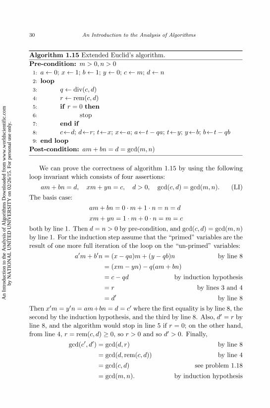
(b) Euclid’s extended algorithm is algorithm 1.15. Note that in the
algorithm, the assignments in line 1 and line 8 are evaluated left to right.
An
Intr
oduc
tion
to th
e A
naly
sis
of A
lgor
ithm
s D
ownl
oade
d fr
om w
ww
.wor
ldsc
ient
ific
.com
by N
AT
ION
AL
UN
ITE
D U
NIV
ER
SIT
Y o
n 02
/26/
15. F
or p
erso
nal u
se o
nly.
April 3, 2012 10:24 World Scientific Book - 9in x 6in soltys˙alg
30 An Introduction to the Analysis of Algorithms
Algorithm 1.15 Extended Euclid’s algorithm.
Pre-condition: m > 0, n > 0
1: a← 0; x← 1; b← 1; y ← 0; c← m; d← n
2: loop
3: q ← div(c, d)
4: r ← rem(c, d)
5: if r = 0 then
6: stop
7: end if
8: c←d; d←r; t←x; x←a; a← t− qa; t←y; y←b; b← t− qb9: end loop
Post-condition: am+ bn = d = gcd(m,n)
We can prove the correctness of algorithm 1.15 by using the following
loop invariant which consists of four assertions:
am+ bn = d, xm+ yn = c, d > 0, gcd(c, d) = gcd(m,n). (LI)
The basis case:
am+ bn = 0 ·m+ 1 · n = n = d
xm+ yn = 1 ·m+ 0 · n = m = c
both by line 1. Then d = n > 0 by pre-condition, and gcd(c, d) = gcd(m,n)
by line 1. For the induction step assume that the “primed” variables are the
result of one more full iteration of the loop on the “un-primed” variables:
a′m+ b′n = (x− qa)m+ (y − qb)n by line 8
= (xm− yn)− q(am+ bn)
= c− qd by induction hypothesis
= r by lines 3 and 4
= d′ by line 8
Then x′m = y′n = am+bn = d = c′ where the first equality is by line 8, the
second by the induction hypothesis, and the third by line 8. Also, d′ = r by
line 8, and the algorithm would stop in line 5 if r = 0; on the other hand,
from line 4, r = rem(c, d) ≥ 0, so r > 0 and so d′ > 0. Finally,
gcd(c′, d′) = gcd(d, r) by line 8
= gcd(d, rem(c, d)) by line 4
= gcd(c, d) see problem 1.18
= gcd(m,n). by induction hypothesis
An
Intr
oduc
tion
to th
e A
naly
sis
of A
lgor
ithm
s D
ownl
oade
d fr
om w
ww
.wor
ldsc
ient
ific
.com
by N
AT
ION
AL
UN
ITE
D U
NIV
ER
SIT
Y o
n 02
/26/
15. F
or p
erso
nal u
se o
nly.

April 3, 2012 10:24 World Scientific Book - 9in x 6in soltys˙alg
Preliminaries 31
For partial correctness it is enough to show that if the algorithm termi-
nates, the post-condition holds. If the algorithm terminates, then r = 0,
so rem(c, d) = 0 and gcd(c, d) = gcd(d, 0) = d. On the other hand,
by (LI), we have that am + bn = d, so am + bn = d = gcd(c, d) and
gcd(c, d) = gcd(m,n).
(c) On pp. 292–293 in [Delfs and Knebl (2007)] there is a nice analysis
of their version of the algorithm. They bound the running time in terms of
Fibonacci numbers, and obtain the desired bound on the running time.
Problem 1.23. For partial correctness of algorithm 1.3, we show that if
the pre-condition holds, and if the algorithm terminates, then the post-
condition will hold. So assume the pre-condition, and suppose first that A
is not a palindrome. Then there exists a smallest i0 (there exists one, and
so by the LNP there exists a smallest one) such that A[i0] 6= A[n− i0 + 1],
and so, after the first i0 − 1 iteration of the while-loop, we know from the
loop invariant that i = (i0 − 1) + 1 = i0, and so line 4 is executed and the
algorithm returns F. Therefore, “A not a palindrome” ⇒ “return F.”
Suppose now that A is a palindrome. Then line 4 is never executed (as
no such i0 exists), and so after the k = bn2 c-th iteration of the while-loop,
we know from the loop invariant that i = bn2 c+ 1 and so the while-loop is
not executed any more, and the algorithm moves on to line 8, and returns T.
Therefore, “A is a palindrome” ⇒ “return T.”
Therefore, the post-condition, “return T iff A is a palindrome,” holds.
Note that we have only used part of the loop invariant, that is we used the
fact that after the k-th iteration, i = k+ 1; it still holds that after the k-th
iteration, for 1 ≤ j ≤ k, A[j] = A[n − j + 1], but we do not need this fact
in the above proof.
To show that the algorithm does actually terminates, let di = bn2 c − i.By the pre-condition, we know that n ≥ 1. The sequence d1, d2, d3, . . . is a
decreasing sequence of positive integers (because i ≤ bn2 c), so by the LNP
it is finite, and so the loop terminates.
Problem 1.24. It is very easy once you realize that in Python the slice
[::-1] generates the reverse string. So, to check whether string s is a
palindrome, all we do is write s == s[::-1].
Problem 1.25. The solution is given by algorithm 1.16.
Let the loop invariant be: “x is a power of 2 iff n is a power of 2.”
We show the loop invariant by induction on the number of iterations
of the main loop. Basis case: zero iterations, and since x ← n, x = n, so
obviously x is a power of 2 iff n is a power of 2. For the induction step,
note that if we ever get to update x, we have x′ = x/2, and clearly x′ is a
An
Intr
oduc
tion
to th
e A
naly
sis
of A
lgor
ithm
s D
ownl
oade
d fr
om w
ww
.wor
ldsc
ient
ific
.com
by N
AT
ION
AL
UN
ITE
D U
NIV
ER
SIT
Y o
n 02
/26/
15. F
or p
erso
nal u
se o
nly.
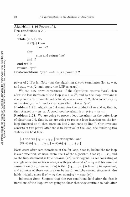
April 3, 2012 10:24 World Scientific Book - 9in x 6in soltys˙alg
32 An Introduction to the Analysis of Algorithms
Algorithm 1.16 Powers of 2.
Pre-condition: n ≥ 1
x← n
while (x > 1) do
if (2|x) then
x← x/2
else
stop and return “no”
end if
end while
return “yes”
Post-condition: “yes” ⇐⇒ n is a power of 2
power of 2 iff x is. Note that the algorithm always terminates (let x0 = n,
and xi+1 = xi/2, and apply the LNP as usual).
We can now prove correctness: if the algorithms returns “yes”, then
after the last iteration of the loop x = 1 = 20, and by the loop invariant n
is a power of 2. If, on the other hand, n is a power of 2, then so is every x,
so eventually x = 1, and so the algorithm returns “yes”.
Problem 1.26. Algorithm 1.4 computes the product of m and n, that is,
the returned z = m · n. A good loop invariant is x · y + z = m · n.
Problem 1.28. We are going to prove a loop invariant on the outer loop
of algorithm 1.6, that is, we are going to prove a loop invariant on the for-
loop (indexed on i) that starts on line 2 and ends on line 7. Our invariant
consists of two parts: after the k-th iteration of the loop, the following two
statements hold true:
(1) the set {v∗1 , . . . , v∗k+1} is orthogonal, and
(2) span{v1, . . . , vk+1} = span{v∗1 , . . . , v∗k+1}.
Basis case: after zero iterations of the for-loop, that is, before the for-loop
is ever executed, we have, from line 1 of the algorithm, that v∗1 ←− v1, and
so the first statement is true because {v∗1} is orthogonal (a set consisting of
a single non-zero vector is always orthogonal—and v∗1 = v1 6= 0 because the
assumption (i.e., pre-condition) is that {v1, . . . , vn} is linearly independent,
and so none of these vectors can be zero), and the second statement also
holds trivially since if v∗1 = v1 then span{v1} = span{v∗1}.Induction Step: Suppose that the two conditions hold after the first k
iterations of the loop; we are going to show that they continue to hold after
An
Intr
oduc
tion
to th
e A
naly
sis
of A
lgor
ithm
s D
ownl
oade
d fr
om w
ww
.wor
ldsc
ient
ific
.com
by N
AT
ION
AL
UN
ITE
D U
NIV
ER
SIT
Y o
n 02
/26/
15. F
or p
erso
nal u
se o
nly.

April 3, 2012 10:24 World Scientific Book - 9in x 6in soltys˙alg
Preliminaries 33
the k + 1 iteration. Consider:
v∗k+2 = vk+2 −k+1∑j=1
µ(k+1)jv∗j ,
which we obtain directly from line 6 of the algorithm; note that the outer
for-loop is indexed on i which goes from 2 to n, so after the k-th execution
of line 2, for k ≥ 1, the value of the index i is k + 1. We show the first
statement, i.e., that {v∗1 , . . . , v∗k+2} are orthogonal. Since, by induction
hypothesis, we know that {v∗1 , . . . , v∗k+1} are already orthogonal, it is enough
to show that for 1 ≤ l ≤ k + 1, v∗l · v∗k+2 = 0, which we do next:
v∗l · v∗k+2 = v∗l ·
vk+2 −k+1∑j=1
µ(k+2)jv∗j
= (v∗l · vk+2)−
k+1∑j=1
µ(k+2)j(v∗l · v∗j )
and since v∗l · v∗j = 0 unless l = j, we have:
= (v∗l · vk+2)− µ(k+2)l(v∗l · v∗l )
and using line 4 of the algorithm we write:
= (v∗l · vk+2)− vk+2 · v∗l‖v∗l ‖2
(v∗l · v∗l ) = 0
where we have used the fact that vl ·vl = ‖vl‖2 and that v∗l ·vk+2 = vk+2 ·v∗l .
For the second statement of the loop invariant we need to show that
span{v1, . . . , vk+2} = span{v∗1 , . . . , v∗k+2}, (1.7)
assuming, by the induction hypothesis, that span{v1, . . . , vk+1} =
span{v∗1 , . . . , v∗k+1}. The argument will be based on line 6 of the algorithm,
which provides us with the following equality:
v∗k+2 = vk+2 −k+1∑j=1
µ(k+2)jv∗j . (1.8)
Given the induction hypothesis, to show (1.7) we need only show the fol-
lowing two things:
(1) vk+2 ∈ span{v∗1 , . . . , v∗k+2}, and
(2) v∗k+2 ∈ span{v1, . . . , vk+2}.
An
Intr
oduc
tion
to th
e A
naly
sis
of A
lgor
ithm
s D
ownl
oade
d fr
om w
ww
.wor
ldsc
ient
ific
.com
by N
AT
ION
AL
UN
ITE
D U
NIV
ER
SIT
Y o
n 02
/26/
15. F
or p
erso
nal u
se o
nly.
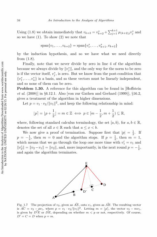
April 3, 2012 10:24 World Scientific Book - 9in x 6in soltys˙alg
34 An Introduction to the Analysis of Algorithms
Using (1.8) we obtain immediately that vk+2 = v∗k+2 +∑k+1j=1 µ(k+2)jv
∗j and
so we have (1). To show (2) we note that
span{v1, . . . , vk+2} = span{v∗1 , . . . , v∗k+1, vk+2}
by the induction hypothesis, and so we have what we need directly
from (1.8).
Finally, note that we never divide by zero in line 4 of the algorithm
because we always divide by ‖v∗j ‖, and the only way for the norm to be zero
is if the vector itself, v∗j , is zero. But we know from the post-condition that
{v∗1 , . . . , v∗n} is a basis, and so these vectors must be linearly independent,
and so none of them can be zero.
Problem 1.30. A reference for this algorithm can be found in [Hoffstein
et al. (2008)] in §6.12.1. Also [von zur Gathen and Gerhard (1999)], §16.2,
gives a treatment of the algorithm in higher dimensions.
Let p = v1 · v2/‖v1‖2, and keep the following relationship in mind:
bpe = bp+1
2c = m ∈ Z ⇐⇒ p ∈ [m− 1
2,m+
1
2) ⊆ R,
where, following standard calculus terminology, the set [a, b), for a, b ∈ R,
denotes the set of all x ∈ R such that a ≤ x < b.
We now give a proof of termination. Suppose first that |p| = 12 . If
p = − 12 , then m = 0 and the algorithm stops. If p = 1
2 , then m = 1,
which means that we go through the loop one more time with v′1 = v1 and
‖v′2‖ = ‖v2−v1‖ = ‖v2‖, and, more importantly, in the next round p = − 12 ,
and again the algorithm terminates.
D’
AB
C
D
E
Fig. 1.7 The projection of v2, given as ~AE, onto v1, given as ~AB. The resulting vector
is ~AC = v2 − pv1, where p = v1 · v2/‖v1‖2. Letting m = bpe, the vector v2 − mv1,is given by ~D′E or ~DE, depending on whether m < p or not, respectively. Of course,
D′ = C = D when p = m.
An
Intr
oduc
tion
to th
e A
naly
sis
of A
lgor
ithm
s D
ownl
oade
d fr
om w
ww
.wor
ldsc
ient
ific
.com
by N
AT
ION
AL
UN
ITE
D U
NIV
ER
SIT
Y o
n 02
/26/
15. F
or p
erso
nal u
se o
nly.
April 3, 2012 10:24 World Scientific Book - 9in x 6in soltys˙alg
Preliminaries 35
If p = m, i.e., p was an integer to begin with (giving ~CE = ~D′E = ~DE
in figure 1.7), then simply by the Pythagorean theorem ‖ ~CE‖ has to be
shorter than ‖ ~AE‖ (as v1, v2 are non-zero, as m 6= 0).
So we may assume that |p| 6= 12 and p 6= m. The two cases where m < p,
giving D′, or m > p, giving D, are symmetric, and so we treat only the
latter case. It must be that |p| > 12 for otherwise m would have been zero,
resulting in termination. Note that ‖ ~CD‖ ≤ 12‖ ~AB‖, because ~AD = m ~AB.
From this and the Pythagorean theorem we know that:
‖ ~AE‖2 = ‖ ~AC‖2 + ‖ ~CE‖2 = p2‖ ~AB‖2 + ‖ ~CE‖2
‖ ~DE‖2 = ‖ ~CD‖2 + ‖ ~CE‖2 ≤ p2‖ ~AB‖2 + ‖ ~CE‖2
and so ‖ ~AE‖2−‖ ~DE‖2 ≥ (p2− 14 )‖ ~AB‖2, and, as we already noted, if the
algorithm does not end in line 6 that means that |p| > 12 , and so it follows
that ‖ ~AE‖ > ‖ ~DE‖, that is, v2 is longer than v2 −mv1, and so the new v2(line 9) is shorter than the old one.
Let v′1, v′2 be the two vectors resulting in one iteration of the loop from
v1, v2. As we noted above, when |p| = 12 termination comes in one or two
steps. Otherwise, ‖v′1‖+‖v′2‖ < ‖v1‖+‖v2‖, and as there are finitely many
pairs of points in a lattice bounded by the sum of the two norms of the
original vectors, and the algorithm ends when one of the vectors becomes
zero, this procedure must end in finitely many steps.
Problem 1.32. Let S ⊆ Z×Z be the set consisting precisely of those pairs
of integers (x, y) such that x ≥ y and x− y is even. We are going to prove
that S is the domain of definition of F . First, if x < y then x 6= y and
so we go on to compute F (x, F (x − 1, y + 1)), and now we must compute
F (x − 1, y + 1); but if x < y, then clearly x − 1 < y + 1; this condition is
preserved, and so we end up having to compute F (x− i, y+ i) for all i, and
so this recursion never “bottoms out.” Suppose that x − y is odd. Then
x 6= y (as 0 is even!), so again we go on to F (x, F (x− 1, y + 1)); if x− y is
odd, so is (x−1)− (y+1) = x−y−2. Again we end up having to compute
F (x− i, y + i) for all i, and so the recursion never terminates. Clearly, all
the pairs in Sc are not in the domain of definition of F .
Suppose now that (x, y) ∈ S. Then x ≥ y and x − y is even; thus,
x− y = 2i for some i ≥ 0. We show, by induction on i, that the algorithm
terminates on such (x, y) and outputs x + 1. Basis case: i = 0, so x = y,
and so the algorithm returns y + 1 which is x + 1. Suppose now that
x − y = 2(i + 1). Then x 6= y, and so we compute F (x, F (x − 1, y + 1)).
But
(x− 1)− (y + 1) = x− y − 2 = 2(i+ 1)− 2 = 2i,
An
Intr
oduc
tion
to th
e A
naly
sis
of A
lgor
ithm
s D
ownl
oade
d fr
om w
ww
.wor
ldsc
ient
ific
.com
by N
AT
ION
AL
UN
ITE
D U
NIV
ER
SIT
Y o
n 02
/26/
15. F
or p
erso
nal u
se o
nly.

April 3, 2012 10:24 World Scientific Book - 9in x 6in soltys˙alg
36 An Introduction to the Analysis of Algorithms
for i ≥ 0, and so by induction F (x − 1, y + 1) terminates and outputs
(x− 1) + 1 = x. So now we must compute F (x, x) which is just x+ 1, and
we are done.
Problem 1.33. We show that f1 is a fixed point of algorithm 1.9. Recall
that in problem 1.32 we showed that the domain of definition of F , the
function computed by algorithm 1.9, is S = {(x, y) : x−y = 2i, i ≥ 0}. Now
we show that if we replace F in algorithm 1.9 by f1, the new algorithm,
which is algorithm 1.17, still computes F albeit not recursively (as f1 is
defined by algorithm 1.10 which is not recursive).
Algorithm 1.17 Algorithm 1.9 with F replaced by f1.
1: if x = y then
2: return y + 1
3: else
4: f1(x, f1(x− 1, y + 1))
5: end if
We proceed as follows: if (x, y) ∈ S, then x − y = 2i with i ≥ 0. On
such (x, y) we know, from problem 1.32, that F (x, y) = x+1. Now consider
the output of algorithm 1.17 on such a pair (x, y). If i = 0, then it returns
y + 1 = x+ 1, so we are done. If i > 0, then it computes
f1(x, f1(x− 1, y + 1)) = f1(x, x) = x+ 1,
and we are done. To see why f1(x− 1, y+ 1) = x notice that there are two
cases: first, if x − 1 = y + 1, then the algorithm for f1 (algorithm 1.10)
returns (y+ 1) + 1 = (x− 1) + 1 = x. Second, if x− 1 > y+ 1 (and that is
the only other possibility), algorithm 1.10 returns (x− 1) + 1 = x as well.
Problem 1.36. After b proposed to g for the first time, whether this
proposal was successful or not, the partners of g could have only gotten
better. Thus, there is no need for b to try again.
Problem 1.37. bs+1 proposes to the girls according to his list of preference;
a g ends up accepting, and if the g who accepted bs+1 was free, she is the new
one with a partner. Otherwise, some b∗ ∈ {b1, . . . , bs} became disengaged,
and we repeat the same argument. The g’s disengage only if a better b
proposes, so it is true that pMs+1(gj) <
j pMs(gj).
Problem 1.38. Suppose that we have a blocking pair {b, g} (meaning that
{(b, g′), (b′, g)} ⊆Mn, but b prefers g to g′, and g prefers b to b′). Either b
came after b′ or before. If b came before b′, then g would have been with
b or someone better when b′ came around, so g would not have become
An
Intr
oduc
tion
to th
e A
naly
sis
of A
lgor
ithm
s D
ownl
oade
d fr
om w
ww
.wor
ldsc
ient
ific
.com
by N
AT
ION
AL
UN
ITE
D U
NIV
ER
SIT
Y o
n 02
/26/
15. F
or p
erso
nal u
se o
nly.

April 3, 2012 10:24 World Scientific Book - 9in x 6in soltys˙alg
Preliminaries 37
engaged to b′. On the other hand, since (b′, g) is a pair, no better offer has
been made to g after the offer of b′, so b could not have come after b′. In
either case we get an impossibility, and so there is no blocking pair {b, g}.Problem 1.39. To show that the matching is boy-optimal, we argue by
contradiction. Let “g is an optimal partner for b” mean that among all the
stable matchings g is the best partner that b can get.
We run the Gale-Shapley algorithm, and let b be the first boy who is
rejected by his optimal partner g. This means that g has already been
paired with some b′, and g prefers b′ to b. Furthermore, g is at least as
desirable to b′ as his own optimal partner (since the proposal of b is the
first time during the run of the algorithm that a boy is rejected by his
optimal partner). Since g is optimal for b, we know (by definition) that
there exists some stable matching S where (b, g) is a pair. On the other
hand, the optimal partner of b′ is ranked (by b′ of course) at most as high
as g, and since g is taken by b, whoever b′ is paired with in S, say g′, b′
prefers g to g′. This gives us an unstable pairing, because {b′, g} prefer
each other to the partners they have in S.
To show that the Gale-Shapley algorithm is girl-pessimal, we use the
fact that it is boy-optimal (which we just showed). Again, we argue by
contradiction. Suppose there is a stable matching S where g is paired
with b, and g prefers b′ to b, where (b′, g) is the result of the Gale-Shapley
algorithm. By boy-optimality, we know that in S we have (b′, g′), where g′
is not higher on the preference list of b′ than g, and since g is already paired
with b, we know that g′ is actually lower. This says that S is unstable since
{b′, g} would rather be together than with their partners.
1.6 Notes
This book is about proving things about algorithms; their correctness, their
termination, their running time, etc. The art of mathematical proofs is a
difficult art to master; a very good place to start is [Velleman (2006)].
N (the set of natural numbers) and IP (the induction principle) are very
tightly related; the rigorous definition of N, as a set-theoretic object, is the
following: it is the unique set satisfying the following three properties: (i) it
contains 0, (ii) if n is in it, then so is n+1, and (iii) it satisfies the induction
principle (which in this context is stated as follows: if S is a subset of N,
and S satisfies (i) and (ii) above, then in fact S = N).
The references in this paragraph are with respect to Knuth’s seminal
The Art of Computer Programming, [Knuth (1997)]. For an extensive study
An
Intr
oduc
tion
to th
e A
naly
sis
of A
lgor
ithm
s D
ownl
oade
d fr
om w
ww
.wor
ldsc
ient
ific
.com
by N
AT
ION
AL
UN
ITE
D U
NIV
ER
SIT
Y o
n 02
/26/
15. F
or p
erso
nal u
se o
nly.
April 3, 2012 10:24 World Scientific Book - 9in x 6in soltys˙alg
38 An Introduction to the Analysis of Algorithms
of Euclid’s algorithm see §1.1. Problem 1.2 comes from §1.2.1, problem #8,
pg. 19. See §2.3.1, pg. 318 for more background on tree traversals. For
the history of the concept of pre and post-condition, and loop invariants,
see pg. 17. In particular, for material related to the extended Euclid’s
algorithm , see page 13, algorithm E, in [Knuth (1997)], page 937 in [Cormen
et al. (2009)], and page 292, algorithm A.5, in [Delfs and Knebl (2007)].
We give a recursive version of the algorithm in section 3.4.
See [Zingaro (2008)] for a book dedicated to the idea of invariants in the
context of proving correctness of algorithms. A great source of problems on
the invariance principle, that is section 1.2, is chapter 1 in [Engel (1998)]
The example about the 8×8 board with two squares missing (figure 1.2)
comes from [Dijkstra (1989)].
The palindrome madamimadam comes from Joyce’s Ulysses.
Section 1.3.5 on the correctness of recursive algorithms is based on chap-
ter 5 of [Manna (1974)].
Section 1.4 is based on §2 in [Cenzer and Remmel (2001)]. For another
presentation of the Stable Marriage problem see chapter 1 in [Kleinberg
and Tardos (2006)]. The reference to the Marquis de Condorcet in the
first sentence of section 1.4 comes from the PhD thesis of Yun Zhai ([Zhai
(2010)]), written under the supervision of Ryszard Janicki. In that thesis,
Yun Zhai references [Arrow (1951)] as the source of the remark regarding
the Marquis de Condorcet’s early attempts at pairwise ranking.
An
Intr
oduc
tion
to th
e A
naly
sis
of A
lgor
ithm
s D
ownl
oade
d fr
om w
ww
.wor
ldsc
ient
ific
.com
by N
AT
ION
AL
UN
ITE
D U
NIV
ER
SIT
Y o
n 02
/26/
15. F
or p
erso
nal u
se o
nly.