9.07 Introduction to Statistics for Brain and Cognitive ... · 9.07 Introduction to ... Understand...
14
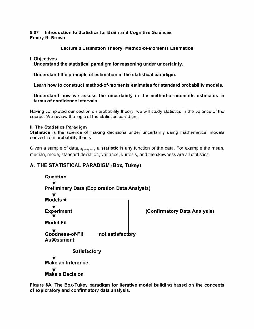
9.07 Introduction to Statistics for Brain and Cognitive Sciences Emery N. Brown Lecture 8 Estimation Theory: Method-of-Moments Estimation I. Objectives Understand the statistical paradigm for reasoning under uncertainty. Understand the principle of estimation in the statistical paradigm. Learn how to construct method-of-moments estimates for standard probability models. Understand how we assess the uncertainty in the method-of-moments estimates in terms of confidence intervals. Having completed our section on probability theory, we will study statistics in the balance of the course. We review the logic of the statistics paradigm. II. The Statistics Paradigm Statistics is the science of making decisions under uncertainty using mathematical models derived from probability theory. Given a sample of data, x 1 ,..., x n , a statistic is any function of the data. For example the mean, median, mode, standard deviation, variance, kurtosis, and the skewness are all statistics. A. THE STATISTICAL PARADIGM (Box, Tukey) Question (Confirmatory Data Analysis) Preliminary Data (Exploration Data Analysis) Models Experiment Model Fit Goodness-of-Fit not satisfactory Assessment Satisfactory Make an Inference Make a Decision Figure 8A. The Box-Tukey paradigm for iterative model building based on the concepts of exploratory and confirmatory data analysis.
-
Upload
duongduong -
Category
Documents
-
view
222 -
download
0
Transcript of 9.07 Introduction to Statistics for Brain and Cognitive ... · 9.07 Introduction to ... Understand...
907 Introduction to Statistics for Brain and Cognitive Sciences Emery N Brown
Lecture 8 Estimation Theory Method-of-Moments Estimation
I Objectives Understand the statistical paradigm for reasoning under uncertainty
Understand the principle of estimation in the statistical paradigm
Learn how to construct method-of-moments estimates for standard probability models
Understand how we assess the uncertainty in the method-of-moments estimates in terms of confidence intervals
Having completed our section on probability theory we will study statistics in the balance of the course We review the logic of the statistics paradigm
II The Statistics Paradigm Statistics is the science of making decisions under uncertainty using mathematical models derived from probability theory
Given a sample of data x1 xn a statistic is any function of the data For example the mean median mode standard deviation variance kurtosis and the skewness are all statistics
A THE STATISTICAL PARADIGM (Box Tukey)
Question
(Confirmatory Data Analysis)
Preliminary Data (Exploration Data Analysis)
Models
Experiment
Model Fit
Goodness-of-Fit not satisfactory Assessment
Satisfactory
Make an Inference
Make a Decision
Figure 8A The Box-Tukey paradigm for iterative model building based on the concepts of exploratory and confirmatory data analysis
page 2 907 Lecture 8 Method-of-Moments Estimation
The Box-Tukey Paradigm (Figure 8A) defines an 8-step approach to experimental design statistical model building and data analysis The iterative cycle of this approach to statistical model building data analysis and inference is attributed to George Box
The initial steps are termed exploratory data analysis (EDA) The idea of EDA was formalized by John Tukey In this phase the statistical model builder uses whatever knowledge is available to propose an initial model or set of models for the data to be analyzed In this phase a set of descriptive usually non-model based statistical tools are used to perform a preliminary analysis of the data This may entail analysis of data from the literature or preliminary data collected in the current laboratory The objective of the EDA phase of the analysis is to develop a set of initial probability models that may be used to describe the stochastic (random) structure in the data The EDA techniques we have learned thus far are data plots histograms five-number summaries stem-and-leaf plots and box plots
Confirmatory data analysis (CDA) uses formal statistical model fitting and assessments of goodness-of-fit to evaluate how well a model fits the data Once a satisfactory fit to the data is obtained as evaluated in a goodness-of-fit assessment the scientist may go ahead to make an inference and then a decision The first part of CDA is proposing an appropriate probability model which is why we just learned a large set of probability models and their properties We now learn how to use these probability models and extensions of them to perform statistical analyses of data We will develop our ability to execute the steps in this paradigm and hence use it to conduct statistical analyses during the next seven weeks
III Method-of-Moments Estimation A What is Estimation
Once a probability model is specified for a given problem the next step is estimation of the model parameters By estimation we mean using a formal procedure to compute the model parameter from the observed data We term any formal procedure that tells us how to compute a model parameter from a sample of data an estimator We term the value computed from the application of the procedure to actual data the estimate
In the next series lectures we will study three methods of estimation method-of-moments maximum likelihood and Bayesian estimation
Example 21 (continued) On the previous day of the learning experiments the animal executed 22 of the 40 trials correctly A reasonable probability model for this problem is the binomial distribution with n = 40 and p unknown if we assume the set of trials to be independent We simply took p the estimate of p to be 22 40 = 055 While this seems reasonable in what sense is this the ldquobestrdquo estimate Is this still the best estimate if the trials are not independent
Example 32 (continued) The MEG measurements appeared Gaussian in shape (Figure 3E) This was further supported by the Q Q plot goodness-of-fit analysis in Figure 3Hminus
The Gaussian distribution has two parameters micro and σ 2 We estimated micro as x sdot minus = minus02 10 11
2 minus22 and ˆ = sdot where σ 20 10
n x nminus1sum x= i
i=1
page 3 907 Lecture 8 Method-of-Moments Estimation
n 2 minus1 2σ = n sum (xi minus x )
i=1
where we recall that x and σ 2 are the sample mean and sample variance respectively
Again are these the best estimates of the parameters The plot of the estimated probability density in Figure 3E and the Q Q plot in Figure 3H suggest that these estimates are very minus reasonable ie highly consistent with the data
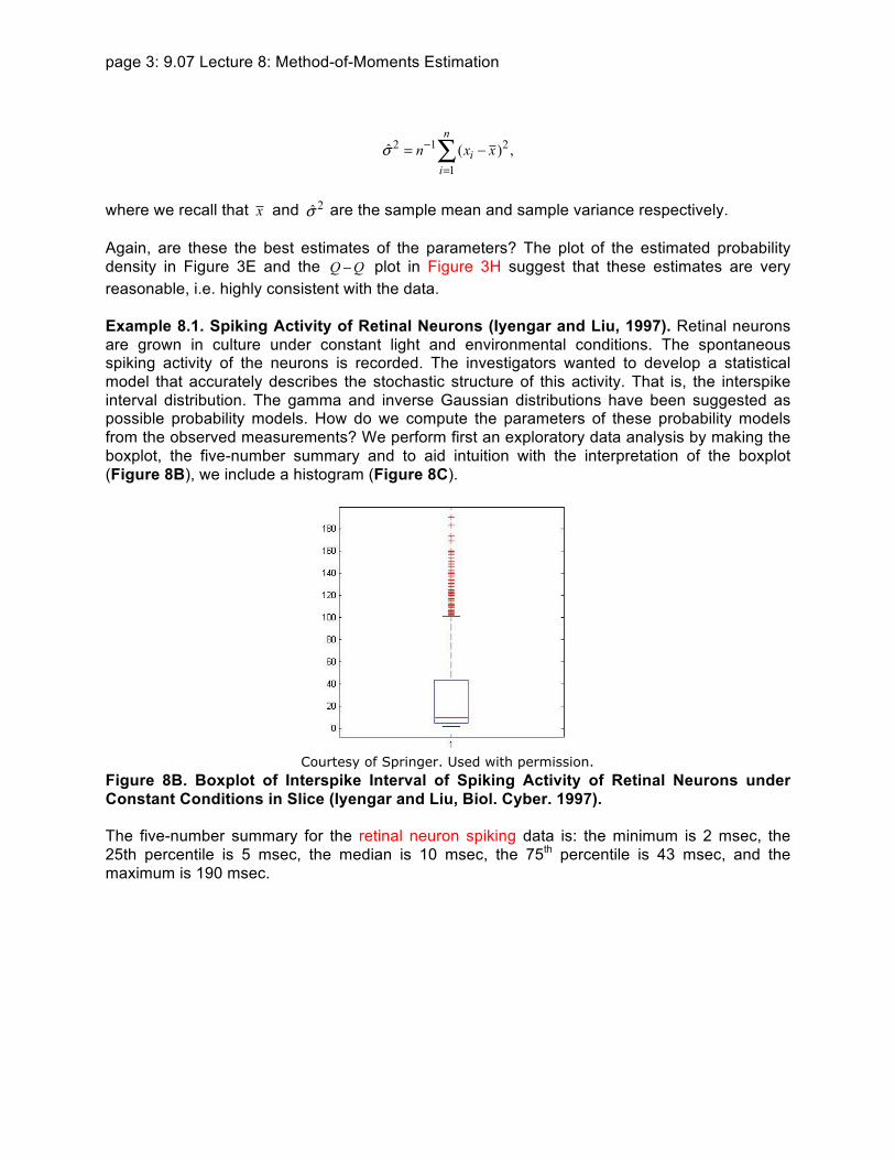
Example 81 Spiking Activity of Retinal Neurons (Iyengar and Liu 1997) Retinal neurons are grown in culture under constant light and environmental conditions The spontaneous spiking activity of the neurons is recorded The investigators wanted to develop a statistical model that accurately describes the stochastic structure of this activity That is the interspike interval distribution The gamma and inverse Gaussian distributions have been suggested as possible probability models How do we compute the parameters of these probability models from the observed measurements We perform first an exploratory data analysis by making the boxplot the five-number summary and to aid intuition with the interpretation of the boxplot (Figure 8B) we include a histogram (Figure 8C)
Figure 8B Boxplot of Interspike Interval of Spiking Activity of Retinal Neurons under Constant Conditions in Slice (Iyengar and Liu Biol Cyber 1997)
The five-number summary for the retinal neuron spiking data is the minimum is 2 msec the 25th percentile is 5 msec the median is 10 msec the 75th percentile is 43 msec and the maximum is 190 msec
Courtesy of Springer Used with permission
page 4 907 Lecture 8 Method-of-Moments Estimation
Figure 8C Interspike Interval Histogram of Spiking Activity of Retinal Neurons under Constant Conditions in Slice (Iyengar and Liu Biol Cyber 1997)
For each of these examples how do we measure the uncertainty in these parameter estimates
B Method-of-Moments Estimation One very straight forward intuitively appealing approach to estimation is the method-of
-moments It is simple to apply Recall that the theoretical moments were defined in Lecture 6 as follows
Given p x ith a probability mass function we define the theoretical moment as( )
micro ii = sum x j p x( j ) (81)
j
ithfor i = 12 and given f x a probability density function we define the theoretical ( )moment as
i = int i ( ) x (82) micro x f x d
for i = 12 These are the moments about zero or the non-central moments Note that the first moment is simply the mean and that the variance is
page 5 907 Lecture 8 Method-of-Moments Estimation
2 ( minus micro)2σ = E x
int 2(x micro) ( ) = minus f x dx
(x2 minus 2micro x + micro2 f x dx (83) = ) ( ) int 2 ( ) minus micro 2 f ( )x dx = x f x dx int int
= micro2 minus micro12
The same result holds for discrete random variables with the integrals changed to summations The variance is the second central moment It is imperative that we add at this point that these definitions only make sense if these moments exist There are certainly cases of probability densities that are well defined for which the moments do not exist One often quoted example is the Cauchy distribution defined as
1f x (84) 2 (1+ x2
( ) = π )
for ( infin infin ) x isin minus
ithGiven a sample of data x1 xn the sample moment is
n minus1 imicroi = n sum xr (85) r=1
for i = 1 23 The sample moments are computed by placing mass of nminus1 at each data point Because all the numbers are finite and the sum is finite the sample moment of each order i exists
Method-of-Moments Estimation Assume we observe x1 xn as a sample from f x θ a( | )probability model with a d minus dimensional unknown parameter θ Assume that the first d moments of ( | ) are finite Equate the theoretical moments to the corresponding sample f x θ moments and estimate θ as the solution to the d minus dimensional equation system
microi ( )θ = microi (86)
for i = 1 d The estimate of θ computed from Eq 86 is the method-of-moments estimate and we denote it as θMM
Example 81 (continued) To fit the gamma probability model to the retinal ganglion cell interspike model using the method-of-moments we consider
micro = ( ) 1 (87) E X = αβ minus
2 2 2σ = E X( minus micro) = αβ minus (88)
page 6 907 Lecture 8 Method-of-Moments Estimation
Note that we have used the second central moment instead of the second moment about zero to simplify the computation Because θ = ( ) α β is 2-dimensional we compute the first sample moment and the second sample central moment as
n x nminus1sum xr (89) =
r=1 n
2 minus1 2σ = n sum (xr minus x) (810) r=1
and our 2-dimensional system of equations is
1x = αβ minus (811)
σ 2 = αβ minus2 (812)
Solving Eqs 811 and 812 yields the method-of-moments estimates
ˆ 2 1β = x ( ) σ minus MM (813)
2 2 1 α = x σ MM ( )minus
Example 21 (continued) To fit the binomial probability model to the rat learning data using the n
minus1sum imethod-of-moments we have = xx n and r=1
x = p (814)
The one-dimensional equation is
= x (815) pMM
and
n minus1 minus1pMM = n sum xr = (40) 22 = 055 (816) r=1
Example 32 (continued) To fit the Gaussian probability model to the MEG noise data using method-of-moments we have simply
microMM = x n (817) 2 minus1 2σMM = n sum(xi minusmicroMM ) r=1
Remark 81 The method-of-moments estimates are simple to compute As we showed they may not exist They are not unique To see this latter point note that we have taken the first d
page 7 907 Lecture 8 Method-of-Moments Estimation
moments to construct the estimation equations but in principle and in practice we could use any d theoretical and d sample moments To see this consider x1 x as a sample from a Poisson n distribution with unknown parameter λ Recall that for a Poisson distribution
( ) = λ (818) E X
and
Var X ( ) = λ (819)
Hence we have
n minus1λMM = micro1 = n sum xr (820) r=1
n n 2 minus1 2 minus1 2λMM = micro2 minus ( )micro1 = n sum xr minus (n sum xr ) (821)
r=1 r=1
Is one of these estimates ldquobetterrdquo We will discuss this further when we discuss maximum likelihood estimation (See Kass Ventura and Brown 2005)
C Uncertainty in the Method-of-Moments Estimate 1 Confidence Interval for the Mean
We computed above the estimate of the probability of a correct response as p = 055 for the learning experiment in Example 21 The method-of-moments procedure requires a justification We certainly do not believe that this is the exact answer There is obvious uncertainty and we would like to quantify that uncertainty This leads us naturally to a discussion of the error in this estimate or alternatively a confidence interval for the true parameter
We recall from the Central Limit Theorem (Lecture 7) that if X1 X is a sample from a n
distribution with mean micro and variance σ 2 then for n large
2σX N (822) n
( micro )
We can use this fact to construct a confidence interval for micro as a way of measuring the
uncertainty in X which for the Example 21 is pMM Assume that σ 2 is known Then from the 12 ( minus micro)n X Central Limit Theorem if we take Z = then we have
σ
page 8 907 Lecture 8 Method-of-Moments Estimation
Pr(| Z |lt 196) = 095 Pr( 196 le Z le 196) = minus
2 1( minus micro)n X Pr( 196 le le 196) = minus σ
minus196 σ 196 σ = Pr( 1 le X minus micro le 1 ) (823) 2 2n n
196 σ minus196 σ = Pr( 1 ge micro minus X ge 1 ) 2 2n n 196 σ 196 σ = Pr( X minus 1 le micro le X + 1 )
2 2n n
Since 196 asymp 2 we have the frequently quoted statement that a 95 confidence interval for the mean of a Gaussian distribution is
2σ 2σX minus 1 le micro le X + 1 (824) 2 2n n
σThe quantity 1
is the standard error (SE) of the mean This is simply an application of Kassrsquo n 2
23-95 rule applied to the Gaussian approximation from the Central Limit Theorem of the distribution of X (Lecture 3)
Remark 82 If the random sample is from a Gaussian distribution then the result is exact
Remark 83 If the random sample is from a binomial distribution (Example 21) then we have σ 2 p(1 minus p)ˆ = and ( ) = Var x = = Hence the approximate 95 confidence interval is p x Var p ( ) n n
p(1 minus p) 12p plusmn 2[ ] (825)
n
For the learning experiment in Example 21 this becomes
055(45) 12055 plusmn 2[ ] (826) 40
055 plusmn 2times 0078
1Hence the confidence interval for p is [0394 0706] Also notice that p(1 minus p) le 4 for all p so that an often used upper bound interval is
1 2p plusmn 2[ ]1 (827)
4n
or
page 9 907 Lecture 8 Method-of-Moments Estimation
1 p plusmn 1 (828) 2n
Example 82 Choosing n to set the length of the confidence interval How many samples should be taken to insure that the length of the 95 confidence interval is less than 01 The
1 1 1 1 p(1 minus p) 1 1 1 2length of the confidence interval is 4[ ]2 le 4[ ]2 = 2[ ]2 If we set 2[ ] = 01 Then we n 4n n n
find that n = 400 Notice that this choice of sample size is independent of the true value of p
Remark 84 If the random sample is from a Poisson distribution then we have that the confidence interval is
ˆ1
λ 2⎛ ⎞λ plusmn 2⎜ ⎟⎜ ⎟ (829)
n⎝ ⎠
What are the conditions for this result to be reasonable
Remark 85 We can construct 90 or 99 confidence intervals or in general intervals of any desired percentage The chosen percentage is the confidence level This is often confused with the significance level of a statistical test These concepts are related but different We will discuss this in Lecture 12 For a 90 confidence interval we have
164σ x plusmn 1 (830) 2n
and for a 99 confidence interval we have
257σ x plusmn 1 (831) 2n
For Gaussian and symmetric distributions we construct the confidence intervals symmetrically In general this need not be the case
2 The Classical Interpretation of the Confidence Interval The classical (frequentist) interpretation of the confidence interval is that stated in terms of the operating characteristics of the confidence interval That is if we were to estimate micro repeatedly with new data then in the long-run (with infinitely many repetitions) about 95 of the time the
2σinterval x plusmn 1 would cover micro In other words if we considered using the procedure again and
2n again it would work in the sense that the confidence we state would correspond more or less to the actual probability that the confidence interval would cover the unknown values of micro
We can illustrate the long-run behavior in a simulation study Let us return to the Example 21 and assume that n = 40 and suppose that the true p = 06 That is the animalrsquos true propensity to respond correctly is 06 It is easy to simulate 10000 Binomial observations from the Binomial distribution with n = 40 and p = 06 We can ask how often does the interval in Eq 825 contain the true value of 06 The simulation takes the following steps
page 10 907 Lecture 8 Method-of-Moments Estimation
1 For i =1 to 10000 Generate Xi Binomial n ( = 40 p = 06) Compute pi = Xi 40
Compute se = ( p (1 minus p ) 40) 12i i i
2 Sum the number of i for which p minus 2se i lt 06 lt pi + 2se i i
We did this and obtained 9454 as the sum in step 2 As a result we conclude that to two-digit accuracy the true value of p is covered by the interval in Eq 825 95 of the time We therefore see the sense in which the standard procedure is well calibrated for large samples
One way probability is often interpreted is in terms of bets if we say an event has probability of 05 this indicates a willingness to take either side of a bet that the event will happen If it has probability 095 this indicates a willingness to take either side of a bet that gives 191 odds the event will happen Here if we were to take either side of a bet that gives 191 odds the that the interval will cover the true value of p in the long run (playing this game a very large number of times) we would expect to neither win nor lose money but rather to more-or-less break even In this sense confidence can be interpreted as making a statement about the operating characteristics of the confidence interval procedure We will review other interpretations of the intervals
3 Confidence Interval for the Variance of a Gaussian Distribution These results have allowed us to compute the approximate distribution of the mean of a
random sample from a distribution with finite mean and variance What is the distribution of the sample variance While we will not answer this question generally we will answer it for the case of a Gaussian distribution If x is a sample from a Gaussian distribution with mean microx x1 2 n
n 2 2 minus1 2and variance σ and we define σ = n sum (xr minus x) then
r=1
2 n 2nσ (xr minus x) 2
σ 2 = sum σ 2
χ( 1nminus ) (832) r=1
We establish the result in the Addendum to Lecture 8 We can use this fact to construct a confidence interval
1 12 nσ 2 σPr( χnminus1(0025) le 2
2 le χnminus1(0975) = Pr( ge
2
2 ge )σ 2 nσ 2χnminus1(0025) χnminus1(0975) (833)
nσ 2 2 nσ 2 = Pr( 2 le σ le 2 )χnminus1(0975) χnminus1(0025)
Remember that the χ 2 distribution with n minus1 degrees of freedom is a gamma distribution with (n minus1) 1α = and β = 2 2
page 11 907 Lecture 8 Method-of-Moments Estimation
D The Gaussian Distribution Revisited When we do not know the value of σ (as is almost always the case) we can estimate it
n minus1 2with the sample standard deviation usually denoted by σ or s = (n minus1) sum (xi minus x ) and use i=1
either of these in place of σ This results in an approximate confidence interval which applies for n large The approximate standard error of the mean x becomes
σ( ) = 1 (834) se x
2n
The approximate 95 confidence interval is
196 σ 196 σX minus 1 le micro le X + 1 (835)
2 2n n
The approximation improves when the data are more nearly Gaussian and may not be as good in moderate sample sizes (say 25 observations) with strongly non-Gaussian data Hence it is important to check the Gaussian assumption with Q Q plots minus
For small samples and Gaussian data it is possible to adjust the confidence intervals for the estimation of σ by s The interval becomes slightly wider than the ldquoexactrdquo interval in Eq 823 We are less certain about micro when there is added uncertainty about σ 2 The correction uses the t minus distribution The t minus distribution is a unimodal symmetric distribution which looks very much like the Gaussian The particular t minus distribution used depends on the sample size used to compute x and s2 The distributions are lower in the middle and have thicker tails than the Gaussian If the sample size is n then ν = n minus1 is the number of degrees of freedom and the appropriate t minus distribution to use is the t minus distribution with ν degrees of freedom Because the tails of the t minus distribution are fatter the value from the t minus distribution corresponding to 196 on the Gaussian distribution will be larger (See Table 81 and Figure 8D) The 95 confidence interval based on the t minus distribution if x is a sample from a Gaussian distribution with x x1 2 n
mean micro and variance σ 2 is
s s x t (836) x t minus 0975 nminus1 1 le micro le + 0975 nminus1 1 2 2n n
As n increases goes to 196 In general as n increases the t minus distribution on ν degrees of t0975 freedom converges to a Gaussian distribution with mean 0 and variance 1
page 12 907 Lecture 8 Method-of-Moments Estimation
ν 0975 10 2228 15 2131 20 2086 25 2060 30 2042 40 2021 60 2000 120 1980 infin 1960
Table 81 The 0975 quantiles of the t-distributions as a function of degrees of freedom
Figure 8D Family of t-distributions plotted as a function of the number of degrees of freedom ν The limiting distribution is the standard Gaussian
For sample sizes of 15 and less the t correction is important
IV Summary Method-of-moments is a simple intuitive approach to estimating the parameters in a probability density We will analyze further the extent to which these methods are ldquobestrdquo once we have studied likelihood theory (Lecture 9) and Bayesian methods (Lecture 10) We will use the bootstrap (Lecture 11) to compute estimates of uncertainty for the method-of-moments estimates
Acknowledgments I am grateful to Uri Eden for making the figures to Jim Mutch for careful proofreading and comments and to Julie Scott for technical assistance Several sections of this lecture have been taken with permission from the class notes for the course Statistical Methods in Neuroscience and Psychology written by Robert Kass in the Department of Statistics at Carnegie Mellon University
page 13 907 Lecture 8 Method-of-Moments Estimation
Textbook Reference DeGroot MH Schervish MJ Probability and Statistics 3rd edition Boston MA Addison
Wesley 2002
Iyengar S Liao Q Modeling neural activity using the generalized inverse Gaussian distribution Biological Cybernetics 1997 77 289ndash295
Rice JA Mathematical Statistics and Data Analysis 3rd edition Boston MA 2007
Literature Reference Kass RE Ventura V Brown EN Statistical issues in the analysis of neuronal data Journal of
Neurophysiology 2005 94 8-25
Website Reference Kass RE Chapter 3 Estimation 2006
MIT OpenCourseWarehttpsocwmitedu
907 Statistics for Brain and Cognitive ScienceFall 2016
For information about citing these materials or our Terms of Use visit httpsocwmiteduterms
page 2 907 Lecture 8 Method-of-Moments Estimation
The Box-Tukey Paradigm (Figure 8A) defines an 8-step approach to experimental design statistical model building and data analysis The iterative cycle of this approach to statistical model building data analysis and inference is attributed to George Box
The initial steps are termed exploratory data analysis (EDA) The idea of EDA was formalized by John Tukey In this phase the statistical model builder uses whatever knowledge is available to propose an initial model or set of models for the data to be analyzed In this phase a set of descriptive usually non-model based statistical tools are used to perform a preliminary analysis of the data This may entail analysis of data from the literature or preliminary data collected in the current laboratory The objective of the EDA phase of the analysis is to develop a set of initial probability models that may be used to describe the stochastic (random) structure in the data The EDA techniques we have learned thus far are data plots histograms five-number summaries stem-and-leaf plots and box plots
Confirmatory data analysis (CDA) uses formal statistical model fitting and assessments of goodness-of-fit to evaluate how well a model fits the data Once a satisfactory fit to the data is obtained as evaluated in a goodness-of-fit assessment the scientist may go ahead to make an inference and then a decision The first part of CDA is proposing an appropriate probability model which is why we just learned a large set of probability models and their properties We now learn how to use these probability models and extensions of them to perform statistical analyses of data We will develop our ability to execute the steps in this paradigm and hence use it to conduct statistical analyses during the next seven weeks
III Method-of-Moments Estimation A What is Estimation
Once a probability model is specified for a given problem the next step is estimation of the model parameters By estimation we mean using a formal procedure to compute the model parameter from the observed data We term any formal procedure that tells us how to compute a model parameter from a sample of data an estimator We term the value computed from the application of the procedure to actual data the estimate
In the next series lectures we will study three methods of estimation method-of-moments maximum likelihood and Bayesian estimation
Example 21 (continued) On the previous day of the learning experiments the animal executed 22 of the 40 trials correctly A reasonable probability model for this problem is the binomial distribution with n = 40 and p unknown if we assume the set of trials to be independent We simply took p the estimate of p to be 22 40 = 055 While this seems reasonable in what sense is this the ldquobestrdquo estimate Is this still the best estimate if the trials are not independent
Example 32 (continued) The MEG measurements appeared Gaussian in shape (Figure 3E) This was further supported by the Q Q plot goodness-of-fit analysis in Figure 3Hminus
The Gaussian distribution has two parameters micro and σ 2 We estimated micro as x sdot minus = minus02 10 11
2 minus22 and ˆ = sdot where σ 20 10
n x nminus1sum x= i
i=1
page 3 907 Lecture 8 Method-of-Moments Estimation
n 2 minus1 2σ = n sum (xi minus x )
i=1
where we recall that x and σ 2 are the sample mean and sample variance respectively
Again are these the best estimates of the parameters The plot of the estimated probability density in Figure 3E and the Q Q plot in Figure 3H suggest that these estimates are very minus reasonable ie highly consistent with the data
Example 81 Spiking Activity of Retinal Neurons (Iyengar and Liu 1997) Retinal neurons are grown in culture under constant light and environmental conditions The spontaneous spiking activity of the neurons is recorded The investigators wanted to develop a statistical model that accurately describes the stochastic structure of this activity That is the interspike interval distribution The gamma and inverse Gaussian distributions have been suggested as possible probability models How do we compute the parameters of these probability models from the observed measurements We perform first an exploratory data analysis by making the boxplot the five-number summary and to aid intuition with the interpretation of the boxplot (Figure 8B) we include a histogram (Figure 8C)
Figure 8B Boxplot of Interspike Interval of Spiking Activity of Retinal Neurons under Constant Conditions in Slice (Iyengar and Liu Biol Cyber 1997)
The five-number summary for the retinal neuron spiking data is the minimum is 2 msec the 25th percentile is 5 msec the median is 10 msec the 75th percentile is 43 msec and the maximum is 190 msec
Courtesy of Springer Used with permission
page 4 907 Lecture 8 Method-of-Moments Estimation
Figure 8C Interspike Interval Histogram of Spiking Activity of Retinal Neurons under Constant Conditions in Slice (Iyengar and Liu Biol Cyber 1997)
For each of these examples how do we measure the uncertainty in these parameter estimates
B Method-of-Moments Estimation One very straight forward intuitively appealing approach to estimation is the method-of
-moments It is simple to apply Recall that the theoretical moments were defined in Lecture 6 as follows
Given p x ith a probability mass function we define the theoretical moment as( )
micro ii = sum x j p x( j ) (81)
j
ithfor i = 12 and given f x a probability density function we define the theoretical ( )moment as
i = int i ( ) x (82) micro x f x d
for i = 12 These are the moments about zero or the non-central moments Note that the first moment is simply the mean and that the variance is
page 5 907 Lecture 8 Method-of-Moments Estimation
2 ( minus micro)2σ = E x
int 2(x micro) ( ) = minus f x dx
(x2 minus 2micro x + micro2 f x dx (83) = ) ( ) int 2 ( ) minus micro 2 f ( )x dx = x f x dx int int
= micro2 minus micro12
The same result holds for discrete random variables with the integrals changed to summations The variance is the second central moment It is imperative that we add at this point that these definitions only make sense if these moments exist There are certainly cases of probability densities that are well defined for which the moments do not exist One often quoted example is the Cauchy distribution defined as
1f x (84) 2 (1+ x2
( ) = π )
for ( infin infin ) x isin minus
ithGiven a sample of data x1 xn the sample moment is
n minus1 imicroi = n sum xr (85) r=1
for i = 1 23 The sample moments are computed by placing mass of nminus1 at each data point Because all the numbers are finite and the sum is finite the sample moment of each order i exists
Method-of-Moments Estimation Assume we observe x1 xn as a sample from f x θ a( | )probability model with a d minus dimensional unknown parameter θ Assume that the first d moments of ( | ) are finite Equate the theoretical moments to the corresponding sample f x θ moments and estimate θ as the solution to the d minus dimensional equation system
microi ( )θ = microi (86)
for i = 1 d The estimate of θ computed from Eq 86 is the method-of-moments estimate and we denote it as θMM
Example 81 (continued) To fit the gamma probability model to the retinal ganglion cell interspike model using the method-of-moments we consider
micro = ( ) 1 (87) E X = αβ minus
2 2 2σ = E X( minus micro) = αβ minus (88)
page 6 907 Lecture 8 Method-of-Moments Estimation
Note that we have used the second central moment instead of the second moment about zero to simplify the computation Because θ = ( ) α β is 2-dimensional we compute the first sample moment and the second sample central moment as
n x nminus1sum xr (89) =
r=1 n
2 minus1 2σ = n sum (xr minus x) (810) r=1
and our 2-dimensional system of equations is
1x = αβ minus (811)
σ 2 = αβ minus2 (812)
Solving Eqs 811 and 812 yields the method-of-moments estimates
ˆ 2 1β = x ( ) σ minus MM (813)
2 2 1 α = x σ MM ( )minus
Example 21 (continued) To fit the binomial probability model to the rat learning data using the n
minus1sum imethod-of-moments we have = xx n and r=1
x = p (814)
The one-dimensional equation is
= x (815) pMM
and
n minus1 minus1pMM = n sum xr = (40) 22 = 055 (816) r=1
Example 32 (continued) To fit the Gaussian probability model to the MEG noise data using method-of-moments we have simply
microMM = x n (817) 2 minus1 2σMM = n sum(xi minusmicroMM ) r=1
Remark 81 The method-of-moments estimates are simple to compute As we showed they may not exist They are not unique To see this latter point note that we have taken the first d
page 7 907 Lecture 8 Method-of-Moments Estimation
moments to construct the estimation equations but in principle and in practice we could use any d theoretical and d sample moments To see this consider x1 x as a sample from a Poisson n distribution with unknown parameter λ Recall that for a Poisson distribution
( ) = λ (818) E X
and
Var X ( ) = λ (819)
Hence we have
n minus1λMM = micro1 = n sum xr (820) r=1
n n 2 minus1 2 minus1 2λMM = micro2 minus ( )micro1 = n sum xr minus (n sum xr ) (821)
r=1 r=1
Is one of these estimates ldquobetterrdquo We will discuss this further when we discuss maximum likelihood estimation (See Kass Ventura and Brown 2005)
C Uncertainty in the Method-of-Moments Estimate 1 Confidence Interval for the Mean
We computed above the estimate of the probability of a correct response as p = 055 for the learning experiment in Example 21 The method-of-moments procedure requires a justification We certainly do not believe that this is the exact answer There is obvious uncertainty and we would like to quantify that uncertainty This leads us naturally to a discussion of the error in this estimate or alternatively a confidence interval for the true parameter
We recall from the Central Limit Theorem (Lecture 7) that if X1 X is a sample from a n
distribution with mean micro and variance σ 2 then for n large
2σX N (822) n
( micro )
We can use this fact to construct a confidence interval for micro as a way of measuring the
uncertainty in X which for the Example 21 is pMM Assume that σ 2 is known Then from the 12 ( minus micro)n X Central Limit Theorem if we take Z = then we have
σ
page 8 907 Lecture 8 Method-of-Moments Estimation
Pr(| Z |lt 196) = 095 Pr( 196 le Z le 196) = minus
2 1( minus micro)n X Pr( 196 le le 196) = minus σ
minus196 σ 196 σ = Pr( 1 le X minus micro le 1 ) (823) 2 2n n
196 σ minus196 σ = Pr( 1 ge micro minus X ge 1 ) 2 2n n 196 σ 196 σ = Pr( X minus 1 le micro le X + 1 )
2 2n n
Since 196 asymp 2 we have the frequently quoted statement that a 95 confidence interval for the mean of a Gaussian distribution is
2σ 2σX minus 1 le micro le X + 1 (824) 2 2n n
σThe quantity 1
is the standard error (SE) of the mean This is simply an application of Kassrsquo n 2
23-95 rule applied to the Gaussian approximation from the Central Limit Theorem of the distribution of X (Lecture 3)
Remark 82 If the random sample is from a Gaussian distribution then the result is exact
Remark 83 If the random sample is from a binomial distribution (Example 21) then we have σ 2 p(1 minus p)ˆ = and ( ) = Var x = = Hence the approximate 95 confidence interval is p x Var p ( ) n n
p(1 minus p) 12p plusmn 2[ ] (825)
n
For the learning experiment in Example 21 this becomes
055(45) 12055 plusmn 2[ ] (826) 40
055 plusmn 2times 0078
1Hence the confidence interval for p is [0394 0706] Also notice that p(1 minus p) le 4 for all p so that an often used upper bound interval is
1 2p plusmn 2[ ]1 (827)
4n
or
page 9 907 Lecture 8 Method-of-Moments Estimation
1 p plusmn 1 (828) 2n
Example 82 Choosing n to set the length of the confidence interval How many samples should be taken to insure that the length of the 95 confidence interval is less than 01 The
1 1 1 1 p(1 minus p) 1 1 1 2length of the confidence interval is 4[ ]2 le 4[ ]2 = 2[ ]2 If we set 2[ ] = 01 Then we n 4n n n
find that n = 400 Notice that this choice of sample size is independent of the true value of p
Remark 84 If the random sample is from a Poisson distribution then we have that the confidence interval is
ˆ1
λ 2⎛ ⎞λ plusmn 2⎜ ⎟⎜ ⎟ (829)
n⎝ ⎠
What are the conditions for this result to be reasonable
Remark 85 We can construct 90 or 99 confidence intervals or in general intervals of any desired percentage The chosen percentage is the confidence level This is often confused with the significance level of a statistical test These concepts are related but different We will discuss this in Lecture 12 For a 90 confidence interval we have
164σ x plusmn 1 (830) 2n
and for a 99 confidence interval we have
257σ x plusmn 1 (831) 2n
For Gaussian and symmetric distributions we construct the confidence intervals symmetrically In general this need not be the case
2 The Classical Interpretation of the Confidence Interval The classical (frequentist) interpretation of the confidence interval is that stated in terms of the operating characteristics of the confidence interval That is if we were to estimate micro repeatedly with new data then in the long-run (with infinitely many repetitions) about 95 of the time the
2σinterval x plusmn 1 would cover micro In other words if we considered using the procedure again and
2n again it would work in the sense that the confidence we state would correspond more or less to the actual probability that the confidence interval would cover the unknown values of micro
We can illustrate the long-run behavior in a simulation study Let us return to the Example 21 and assume that n = 40 and suppose that the true p = 06 That is the animalrsquos true propensity to respond correctly is 06 It is easy to simulate 10000 Binomial observations from the Binomial distribution with n = 40 and p = 06 We can ask how often does the interval in Eq 825 contain the true value of 06 The simulation takes the following steps
page 10 907 Lecture 8 Method-of-Moments Estimation
1 For i =1 to 10000 Generate Xi Binomial n ( = 40 p = 06) Compute pi = Xi 40
Compute se = ( p (1 minus p ) 40) 12i i i
2 Sum the number of i for which p minus 2se i lt 06 lt pi + 2se i i
We did this and obtained 9454 as the sum in step 2 As a result we conclude that to two-digit accuracy the true value of p is covered by the interval in Eq 825 95 of the time We therefore see the sense in which the standard procedure is well calibrated for large samples
One way probability is often interpreted is in terms of bets if we say an event has probability of 05 this indicates a willingness to take either side of a bet that the event will happen If it has probability 095 this indicates a willingness to take either side of a bet that gives 191 odds the event will happen Here if we were to take either side of a bet that gives 191 odds the that the interval will cover the true value of p in the long run (playing this game a very large number of times) we would expect to neither win nor lose money but rather to more-or-less break even In this sense confidence can be interpreted as making a statement about the operating characteristics of the confidence interval procedure We will review other interpretations of the intervals
3 Confidence Interval for the Variance of a Gaussian Distribution These results have allowed us to compute the approximate distribution of the mean of a
random sample from a distribution with finite mean and variance What is the distribution of the sample variance While we will not answer this question generally we will answer it for the case of a Gaussian distribution If x is a sample from a Gaussian distribution with mean microx x1 2 n
n 2 2 minus1 2and variance σ and we define σ = n sum (xr minus x) then
r=1
2 n 2nσ (xr minus x) 2
σ 2 = sum σ 2
χ( 1nminus ) (832) r=1
We establish the result in the Addendum to Lecture 8 We can use this fact to construct a confidence interval
1 12 nσ 2 σPr( χnminus1(0025) le 2
2 le χnminus1(0975) = Pr( ge
2
2 ge )σ 2 nσ 2χnminus1(0025) χnminus1(0975) (833)
nσ 2 2 nσ 2 = Pr( 2 le σ le 2 )χnminus1(0975) χnminus1(0025)
Remember that the χ 2 distribution with n minus1 degrees of freedom is a gamma distribution with (n minus1) 1α = and β = 2 2
page 11 907 Lecture 8 Method-of-Moments Estimation
D The Gaussian Distribution Revisited When we do not know the value of σ (as is almost always the case) we can estimate it
n minus1 2with the sample standard deviation usually denoted by σ or s = (n minus1) sum (xi minus x ) and use i=1
either of these in place of σ This results in an approximate confidence interval which applies for n large The approximate standard error of the mean x becomes
σ( ) = 1 (834) se x
2n
The approximate 95 confidence interval is
196 σ 196 σX minus 1 le micro le X + 1 (835)
2 2n n
The approximation improves when the data are more nearly Gaussian and may not be as good in moderate sample sizes (say 25 observations) with strongly non-Gaussian data Hence it is important to check the Gaussian assumption with Q Q plots minus
For small samples and Gaussian data it is possible to adjust the confidence intervals for the estimation of σ by s The interval becomes slightly wider than the ldquoexactrdquo interval in Eq 823 We are less certain about micro when there is added uncertainty about σ 2 The correction uses the t minus distribution The t minus distribution is a unimodal symmetric distribution which looks very much like the Gaussian The particular t minus distribution used depends on the sample size used to compute x and s2 The distributions are lower in the middle and have thicker tails than the Gaussian If the sample size is n then ν = n minus1 is the number of degrees of freedom and the appropriate t minus distribution to use is the t minus distribution with ν degrees of freedom Because the tails of the t minus distribution are fatter the value from the t minus distribution corresponding to 196 on the Gaussian distribution will be larger (See Table 81 and Figure 8D) The 95 confidence interval based on the t minus distribution if x is a sample from a Gaussian distribution with x x1 2 n
mean micro and variance σ 2 is
s s x t (836) x t minus 0975 nminus1 1 le micro le + 0975 nminus1 1 2 2n n
As n increases goes to 196 In general as n increases the t minus distribution on ν degrees of t0975 freedom converges to a Gaussian distribution with mean 0 and variance 1
page 12 907 Lecture 8 Method-of-Moments Estimation
ν 0975 10 2228 15 2131 20 2086 25 2060 30 2042 40 2021 60 2000 120 1980 infin 1960
Table 81 The 0975 quantiles of the t-distributions as a function of degrees of freedom
Figure 8D Family of t-distributions plotted as a function of the number of degrees of freedom ν The limiting distribution is the standard Gaussian
For sample sizes of 15 and less the t correction is important
IV Summary Method-of-moments is a simple intuitive approach to estimating the parameters in a probability density We will analyze further the extent to which these methods are ldquobestrdquo once we have studied likelihood theory (Lecture 9) and Bayesian methods (Lecture 10) We will use the bootstrap (Lecture 11) to compute estimates of uncertainty for the method-of-moments estimates
Acknowledgments I am grateful to Uri Eden for making the figures to Jim Mutch for careful proofreading and comments and to Julie Scott for technical assistance Several sections of this lecture have been taken with permission from the class notes for the course Statistical Methods in Neuroscience and Psychology written by Robert Kass in the Department of Statistics at Carnegie Mellon University
page 13 907 Lecture 8 Method-of-Moments Estimation
Textbook Reference DeGroot MH Schervish MJ Probability and Statistics 3rd edition Boston MA Addison
Wesley 2002
Iyengar S Liao Q Modeling neural activity using the generalized inverse Gaussian distribution Biological Cybernetics 1997 77 289ndash295
Rice JA Mathematical Statistics and Data Analysis 3rd edition Boston MA 2007
Literature Reference Kass RE Ventura V Brown EN Statistical issues in the analysis of neuronal data Journal of
Neurophysiology 2005 94 8-25
Website Reference Kass RE Chapter 3 Estimation 2006
MIT OpenCourseWarehttpsocwmitedu
907 Statistics for Brain and Cognitive ScienceFall 2016
For information about citing these materials or our Terms of Use visit httpsocwmiteduterms
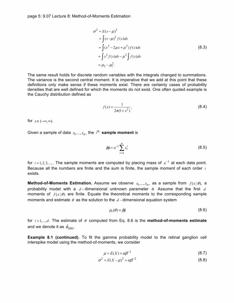
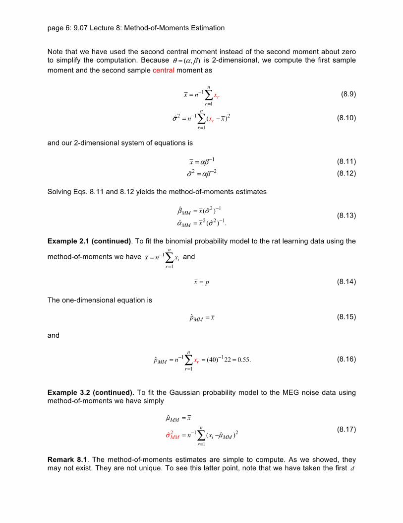
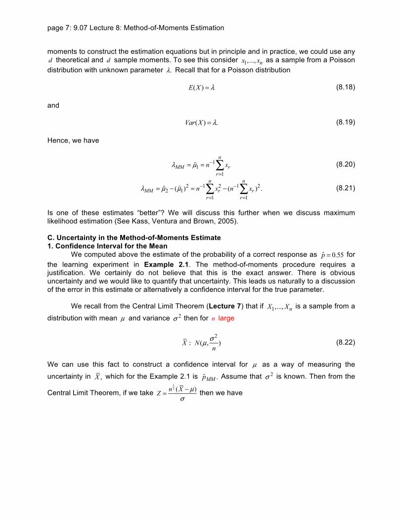
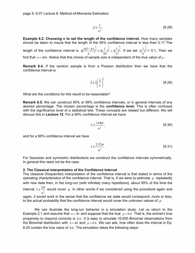
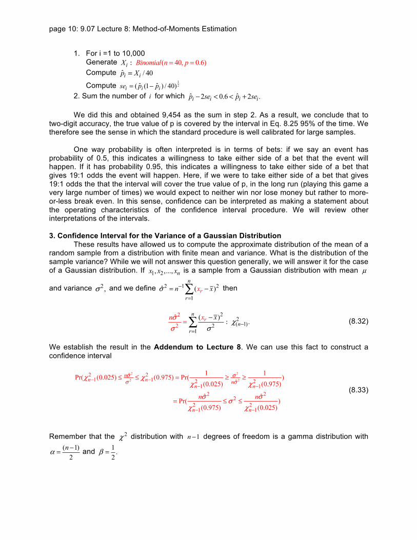
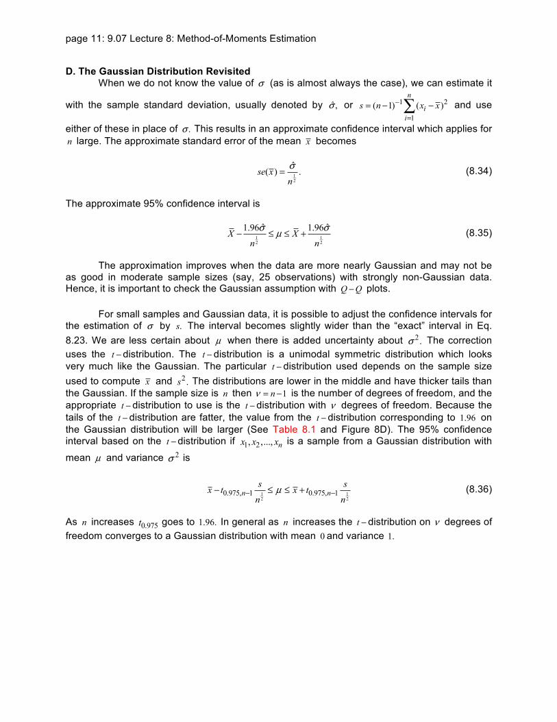
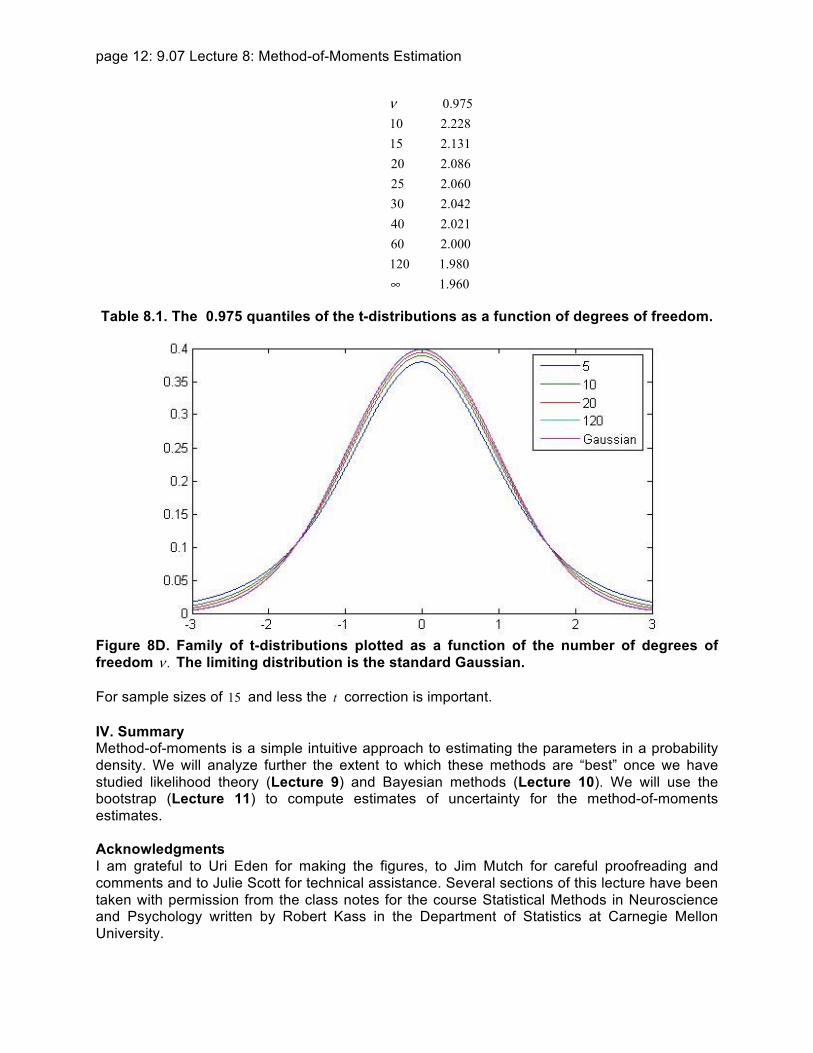

MIT OpenCourseWarehttpsocwmitedu
907 Statistics for Brain and Cognitive ScienceFall 2016
For information about citing these materials or our Terms of Use visit httpsocwmiteduterms