9 The conservation theorems: Lecture 23

9.1 Energy Conservation

(a) For energy to be conserved we expect that the total energy density (energy per volume ) utot to obeya conservation law

∂tutot + ∂iSitot = 0 (9.1)

where Stot is the total energy flux.

(b) We divide the energy density into a mechanical energy density umech (e.g. dU = T dS − p dV ) and anelectromagnetic energy density uem

utot = umech + uem (9.2)

where

uem =1

2E ·D +

1

2H ·B (9.3)

(c) The energy flux S is also divided into a mechanical energy flux and an electromagnetic energy flux

Stot = Smech + Sem (9.4)

where the mechanical energy flux comes from forces between the different mechanical subsystem and

Sem = cE ×H (9.5)

(d) In this way for a mechanically isolated system U =∫udV

dUmech

dt+dUem

dt= −

∫∂V

S · da (9.6)

(e) The starting point of this derivation is

∂tumech + ∂iSimech = j ·E (9.7)

and showing that

j ·E = −∂tuem − ∂iSiem (9.8)

9.2 Momentum Conservation

(a) For momentum to be conserved we expect that the total momentum per volume gtot satisfies a con-servation law

∂tgj + ∂iT

ijtot = 0 (9.9)

where T ij is the total stress tensor

33

34 CHAPTER 9. THE CONSERVATION THEOREMS: LECTURE 23

(b) We divide the momentum density into a mechanical momentum density gmech and an electromagneticmomentum density gem

gtot = gmech + gem (9.10)

where the electromagnetic momentum density is

gem = D ×B =µε

c2S . (9.11)

The last step is valid for simple matter and µε/c2 = (n/c)2 where n =√µε is the index of refraction.

(c) The stress tensor T ijtot is also divided into a mechanical stress tensor T ijmech and an electromagneticstress T ijem

T ijtot = T ijmech + T ijem (9.12)

where the mechanical stress comes from the forces between the different mechanical subsystem and

T ijem =− 12 (DiEj +DjEi) + 1

2D ·Eδij︸ ︷︷ ︸

electric stress

+ − 12 (HiBj +BjHi) + 1

2H ·Bδij︸ ︷︷ ︸

magnetic stress

(9.13)

= ε(−EiEj + 1

2E2δij

)︸ ︷︷ ︸

electric

+1

µ

(−BiBj + 1

2B2δij

)︸ ︷︷ ︸

magnetic

(9.14)

(d) In this way for a mechanically isolated system the total momentum P =∫g dV

dP jmech

dt+dP jem

dt= −

∫∂V

da niTij (9.15)

(e) The starting point of this derivation is

∂tgjmech + ∂iT

ijmech = ρEj + (j/c×B)j (9.16)

and showing thatρEj + (j/c×B)j = −∂tgjem − ∂iT ijem (9.17)

9.3 Angular momentum conservation

(a) Given the symmetry of stress tensor T ij = T ji and the conservation law

∂tgjtot + ∂iT

ijtot = 0 (9.18)

Then one can prove that angular momentum density satisfies a conservation law

∂t(r × gtot)i + ∂`(εijkrjT k`tot) = 0 (9.19)

where the total angular momentum density is r × gtot

(b) The angular momentum is divided into its mechanical and electromagnetic pieces. The electromagneticpiece is:

Lem =

∫V

r × gem (9.20)

(c) For a mechanically isolated system we have

d

dt(Lmech +Lem)i = −

∫∂V

dan` εijkrjT k`em︸ ︷︷ ︸

em torque on the system

(9.21)

10 Waves

10.1 Plane waves and the Helmhotz Equation: Lecture 24

(a) We look for solutions which have a particular (eigen)-frequency dependence ωn, E = En(x)e−iωnt.This is very similar to the way that we look for particular energies in quantum mechanics, going fromthe time-dependent Schrodinger equation to the time-independent Schrodinger equation.

∇ ·Dn(x) =0 (10.1)

∇×Hn(x) =−iωnD(x)

c(10.2)

∇×Bn(x) =0 (10.3)

∇×En(x) =iωnB(x)

c(10.4)

From which we deduce the Helmholtz equation(∇2 +

ω2n µε

c2

)En =0 (10.5)(

∇2 +ω2n µε

c2

)Hn =0 (10.6)

which is an equation for the eigen-frequencies ωn and the corresponding solutions Hn(x),En(x). It isimportant to emphasize that for a bounded system not all frequencies will be possible and still satisfythe boundary conditions.

The general solution is a superposition of these eigen modes,

E(t,x) =∑n

CnEn(x)e−iωnt (10.7)

where the (complex) coefficients are adjusted to match the initial amplitude and time derivative of thewave. As in quantum mechanics the eigen functions, are of interest in their own right.

We will drop the n sub label on the wave-functions and eigen-frequencies below.

(b) If we restrict our wave functions to have the form En(r) ≡ Ek(r)

Ek(r) = ~E eik·r (10.8)

Bk(r) = ~Beik·r (10.9)

then we get a condition on the frequency

k2 =ω2µε

c2or ω(k) =

c√µε

k (10.10)

We have not assumed that ~E , ~B, or k are real.

35

36 CHAPTER 10. WAVES

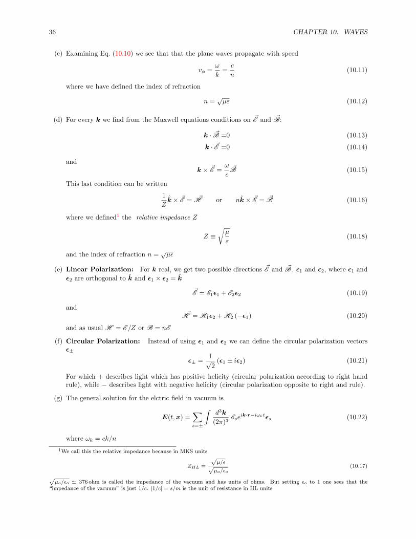
(c) Examining Eq. (10.10) we see that that the plane waves propagate with speed

vφ =ω

k=c

n(10.11)

where we have defined the index of refraction

n =√µε (10.12)

(d) For every k we find from the Maxwell equations conditions on ~E and ~B:

k · ~B =0 (10.13)

k · ~E =0 (10.14)

andk × ~E =

ω

c~B (10.15)

This last condition can be written

1

Zk × ~E = ~H or nk × ~E = ~B (10.16)

where we defined1 the relative impedance Z

Z ≡√µ

ε(10.18)

and the index of refraction n =√µε

(e) Linear Polarization: For k real, we get two possible directions ~E and ~B. ε1 and ε2, where ε1 and

ε2 are orthogonal to k and ε1 × ε2 = k

~E = E1ε1 + E2ε2 (10.19)

and~H = H1ε2 + H2 (−ε1) (10.20)

and as usual H = E /Z or B = nE

(f) Circular Polarization: Instead of using ε1 and ε2 we can define the circular polarization vectorsε±

ε± =1√2

(ε1 ± iε2) (10.21)

For which + describes light which has positive helicity (circular polarization according to right handrule), while − describes light with negative helicity (circular polarization opposite to right and rule).

(g) The general solution for the elctric field in vacuum is

E(t,x) =∑s=±

∫d3k

(2π)3Ese

ik·r−iωktεs (10.22)

where ωk = ck/n

1We call this the relative impedance because in MKS units

ZHL =

√µ/ε√µo/εo

(10.17)

√µo/εo ' 376 ohm is called the impedance of the vacuum and has units of ohms. But setting εo to 1 one sees that the

“impedance of the vacuum” is just 1/c. [1/c] = s/m is the unit of resistance in HL units

10.1. PLANE WAVES AND THE HELMHOTZ EQUATION: LECTURE 24 37

(h) Power and Energy Transport

i) For a general wave satisfying the Helmholtz equation (i.e. sunusoidal) we have the time averagedpoynting flux

Sav(r) =1

2Re[cE(r)×H∗(r)

](10.23)

ii) For a general wave satisfying the Helmholtz equation (i.e. sunusoidal) we have the time averagedenergy density :

uav(r) =1

2Re

[1

2εE ·E∗ +

1

2µB ·B∗

](10.24)

iii) For a plane wave we have

uav = 12ε| ~E |

2 (10.25)

Sav =c

Z| ~E |2 k (10.26)

=c

nuav k (10.27)

38 CHAPTER 10. WAVES

10.2 Reflection at interfaces: Lecture 25 and 26

Reflection at a Dielectric: Lecture 25

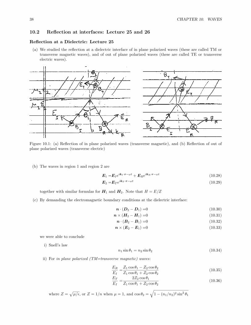
(a) We studied the reflection at a dielectric interface of in plane polarized waves (these are called TM ortransverse magnetic waves), and of out of plane polarized waves (these are called TE or transverseelectric waves).

Figure 10.1: (a) Reflection of in plane polarized waves (transverse magnetic), and (b) Reflection of out ofplane polarized waves (transverse electric)

(b) The waves in region 1 and region 2 are

E1 =EIeikI ·r−ωt +ERe

ikR·r−ωt (10.28)

E2 =ET eikT ·r−ωt (10.29)

together with similar formulas for H1 and H2. Note that H = E/Z

(c) By demanding the electromagnetic boundary conditions at the dielectric interface:

n · (D2 −D1) =0 (10.30)

n× (H2 −H1) =0 (10.31)

n · (B2 −B1) =0 (10.32)

n× (E2 −E1) =0 (10.33)

we were able to conclude

i) Snell’s law

n1 sin θ1 = n2 sin θ2 (10.34)

ii) For in plane polarized (TM=transverse magnetic) waves:

EREI

=Z1 cos θ1 − Z2 cos θ2

Z1 cos θ1 + Z2 cos θ2(10.35)

ETEI

=2Z2 cos θ1

Z1 cos θ1 + Z2 cos θ2(10.36)

where Z =√µ/ε, or Z = 1/n when µ = 1, and cos θ2 =

√1− (n1/n2)2 sin2 θ1

10.2. REFLECTION AT INTERFACES: LECTURE 25 AND 26 39

iii) For out of plane polarized (TE=transverse electric) waves:

EREI

=Z2 cos θ1 − Z1 cos θ2

Z2 cos θ1 + Z1 cos θ2(10.37)

ETEI

=2Z2 cos θ1

Z2 cos θ1 + Z1 cos θ2(10.38)

iv) You should feel comfortable deriving these results.

(d) The reflection coefficient of in-plane (TM) waves vanishes at the Brewster angle tan θB = n1/n2. Thismeans that upon reflection the light will be partially polarized.

Reflection at Metallic interface: Lecture 26

(a) Compare the constituent relation for a metal and a dielectric:

j =σE + χe∂tE + cχBm∇×B Metal (10.39)

j = χe∂tE + cχBm∇×B Dielectric , (10.40)

in Fourier space

j =− iωE( iσω

+ χe

)+ cχBm∇×B Metal (10.41)

j =− iωE(χe

)cχBm∇×B Dielectric , (10.42)

Thus (noting that ε = 1 + χe) we see that the Maxwell equations in a metal merely involve thereplacement χe → χe + iσ/ω, or

ε→ ε(ω) = ε+iσ

ω(10.43)

Usually σ/ω � ε and thus usually we replace:

ε→ ε(ω) ' iσ

ω(10.44)

(b) By looking for solutions of the form H = Hceik·r−ıωt in metal, we found kmetal

± = ±(1 + i)/δ, so for awave propagating in the z direction the decaying amplitude is

H = Hceikmetal

± z = Hceiz/δe−z/δ (10.45)

we also found the (much smaller) electric field

E =

√µω

σ

(1− i)√2Hce

iz/δe−z/δ (10.46)

which is suppressed by√ω/σ relative to H

(c) We used these to study the reflection of light at a metal surface of high conductivity at normal incidence.This involves writing the fields outside the metal as a superposition of an ingoing and outgoing wave,and applying the boundary conditions as in the previous section to match the wave solutions acrossthe interface. You should feel comfortable deriving these results.

(d) We analyzed the power flow in the reflection of light by the metal, and we analyzed the wave packetdynamics (see next section).

40 CHAPTER 10. WAVES

10.3 Waves in dielectrics and metals, dispersion

General Theory

(a) For maxwell equations at higher frequency the gradient expansion that we used should be replaced,as the frequency of the light is not small compared to atomic frequencies. However the wavelength λis typically still much longer than the spacing between atoms, λ� ao. Thus the expansion in spatialderivatives is still a good expansion. In a linear response approximation we write the current as anexpansion:

j(t, r) =

∫ ∞∞

dt′ σ(t− t′)E(t′, r) +

∫dt′χBm(t− t′) c∇×B(t′, r)︸ ︷︷ ︸

often neglect

(10.47)

Often the magnetic response (which is smaller by (v/c)2) is neglected.

(b) The functions are causal, we want them to vanish for t′ > t, yielding

σ(t) =0 t < 0 (10.48)

χBm(t) =0 t < 0 (10.49)

(c) In frequency space the consituitent relation reads

j(ω, r) = σ(ω)E(ω, r) + χBm(ω) c∇×B(ω, r)︸ ︷︷ ︸usually neglect

(10.50)

Motivated by considerations described below we will write the same function σ(ω) in a variety of ways

σ(ω) ≡ −iωχe(ω) and ε(ω) ≡ 1 + χe(ω) ≡ 1 + iσ(ω)

ω(10.51)

(d) For low frequencies (less than an inverse collision timescale ω � 1/τc) our previous work applies. Thisthis places constraints on σ(ω) at low frequencies

i) For a conductor for ω � τc, we need that j(t) = σoE(t). This means that

σ(ω) ' σo for ω → 0 (10.52)

ii) For an insulator (dielectric) we had that j(t) = ∂tP (t) = χe ∂tE so we expect that

σ(ω) ' −iωχe for ω → 0 (10.53)

It is this different low frequency behavior of the conductivity that distinguishes a conductor from aninsulator.

(e) With consituitive relation given in Eq. (10.50), and the continuity equation −iωρ(ω) = −∇ · j(ω, r),we find that the maxwell equations in matter are formally the same as at low frequenency

ε(ω)∇ ·E(ω, r) =0 (10.54)

∇×B(ω, r) =−iωε(ω)µ(ω)

cE(ω) (10.55)

∇ ·B(ω, r) =0 (10.56)

∇×E(ω, r) =iω

cB(ω, r) (10.57)

ε(ω) and µ(ω) are complex functions of ω

ε(ω) =1 + χe(ω) (10.58)

µ(ω) =1

1− χBm(ω)(10.59)

We gave two models for what ε(ω) might look like in dielectrics and metals (see below).

10.3. WAVES IN DIELECTRICS AND METALS, DISPERSION 41

(f) Given the Maxwell equations we studied the propagation of transverse waves

ET (t, r) = Eoeik·x−ıωt (10.60)

with Eo · k = 0. The helmholtz equation for transverse waves becomes:[−k2 +

ω2ε(ω)µ(ω)

c2

]Eo = 0 . (10.61)

where ε(ω) ≡ ε′(ω) + iε′′(ω) and µ(ω) = µ′(ω) + iµ′′(ω) are complex functions of frequency, with realparts, ε′(ω), µ′(ω), and imaginary parts, ε′′(ω), µ′′(ω). In general Eq. (10.61) determines to a relationbetween ω(k) and k for any specified ε(ω) and µ(ω). Usually we will set µ(ω) = 1.

(g) The real part of ω(k) is known as the dispersion curve and determines the phase and group velocities ofthe wave and wave packets. This is determined by the real part of the permitivity ε(ω). The imaginarypart of the ε(ω) dtermines the absorption of the wave.

To see this we solved Eq. (10.61) with µ(ω) = 1 and the imaginary part of ε(ω) small. Defining

ω(k) ≡ ωo(k)− i2Γ(k) , (10.62)

so thatET (t,x) = Eoe

ik·xeiωo(k)te−12

Γ(k)t (10.63)

we find that ωo(k) (which is known as the dispersion curve is) satisfies

− k2 +ω2o

c2ε′(ωo) = 0 (10.64)

and the damping rate is

Γ(k) =ωo(k)ε′′(ωo(k))

ε′(ωo(k))(10.65)

(h) Sometimes it is easier to think about it as k as function of ω rather than ω(k). Solving Eq. (10.61) fork

k =ω

cn(ω) , (10.66)

with n(ω) =√ε(ω), we find the wave form:

E(t, r) = Eoe−iωt+ik·x = Eo e

−iωt eiωn1(ω)

c ze−ωn2(ω)

c z (10.67)

where n1(ω) is the real part of n(ω), and n2(ω) is the imaginary part of n(ω).

Thus the real part of n(ω) determines the real wave number of the wave, (ω/c)n1(ω), while theimaginary part of n(ω), n2(ω), determines the absorption of the wave as it propagates through media.

A model ε(ω) function for dielectrics

In general one needs to know how the medium reacts in order to determine σ(ω). At low frequency σ(ω)is determined by a few constants which are given by the taylor expansion of σ(ω). At higher frequencya detailed micro-theory is needed to compute σ(ω). The following model capture the qualitative featuresof dielectrics as a function of frequency. Replacing the model for a dielectric, with a quantum mechanicaldescription of electronic oscillations in atoms, gives a realistic description of neutral gasses.

(a) For an insulator we gave a simple model for the dielectric, where the electrons are harmonically boundto the atoms. The equation of motion satisfied by the electrons are

md2x

dt2+mη

dx

dt+mω2

ox = eEext(t) (10.68)

42 CHAPTER 10. WAVES

Solving for the current j(t) = jωe−iωt, with a sinusoidal field E(t) = Eωe

iωt we found χe(ω)

ε(ω) = 1 + χe(ω) = 1 +ω2p

−ω2 + ω2o − iωη

(10.69)

where the plasma frequency is

ω2p =

ne2

m(10.70)

and at low frequency we recover Eq. (4.20)

χe 'ω2p

ω2o

for ω → 0 (10.71)

10.4. DYNAMICS OF WAVE PACKETS 43

10.4 Dynamics of wave packets

(a) Any real wave is a superposition of plane waves:

u(x, t) =

∫ ∞−∞

dk

2πA(k)eikx−ω(k)t (10.72)

The complex values of A(k) can be adjusted so that at time t = 0 the initial conditions, u(x, 0) and∂tu(x, 0), can be satisfied.

(b) A proto-typical wave packet at time t = 0 is a Gaussian packet

u(x, 0) = eikox1√

2πσ2e

(x−xo)2

2σ2 (10.73)

The spatial width is

∆x =σ√2

(10.74)

The Fourier transform isA(k) = exp(− 1

2 (k − ko)2σ2) (10.75)

The wavenumber width

∆k =1√2σ

(10.76)

so

∆k∆x =1

2(10.77)

which saturates the uncertainty bound ∆x∆k ≥ 12 . The Gaussian is the unique wave form which

saturates the bound.

A picture of these Fourier Transforms is

-0.2

-0.15

-0.1

-0.05

0

0.05

0.1

0.15

0.2

-10 -5 0 5 10

Re u

(x,0

)

x

ko = 10

2∆x 0

0.2

0.4

0.6

0.8

1

0 2 4 6 8 10 12 14

A(k

)

k

ko = 10

2∆k

(c) The uncertainty relation relates the wavenumber and spatial widths

∆x∆k ≥ 12 (10.78)

where

(∆x)2 =

∫∞−∞ |u(x, 0)|2(x− x)2∫∞

∞ |u(x, 0)|2(10.79)

(∆k)2 =

∫∞−∞ |A(k)|2(k − k)2∫∞

∞ |A(k)|2(10.80)

44 CHAPTER 10. WAVES

(d) You should be able to derive that the center of the wave packet moves with the group velocity

vg =dω

dk(10.81)

In a very similar way one derives that, if a wave experiences a frequency dependent phase shift φ(ω)upon reflection or transmission, the wave packet will be delayed relative to a geometric optics approx-imation by a time delay

∆ =dφ(ω)

dω(10.82)