9. Sampling Distributions

Prerequisites• none

A. IntroductionB. Sampling Distribution of the MeanC. Sampling Distribution of Difference Between MeansD. Sampling Distribution of Pearson's rE. Sampling Distribution of a ProportionF. ExercisesThe concept of a sampling distribution is perhaps the most basic concept in inferential statistics. It is also a difficult concept because a sampling distribution is a theoretical distribution rather than an empirical distribution.

The introductory section defines the concept and gives an example for both a discrete and a continuous distribution. It also discusses how sampling distributions are used in inferential statistics.

The remaining sections of the chapter concern the sampling distributions of important statistics: the Sampling Distribution of the Mean, the Sampling Distribution of the Difference Between Means, the Sampling Distribution of r, and the Sampling Distribution of a Proportion.

300

Introduction to Sampling Distributionsby David M. Lane

Prerequisites• Chapter 1: Distributions• Chapter 1: Inferential Statistics

Learning Objectives1. Define inferential statistics2. Graph a probability distribution for the mean of a discrete variable3. Describe a sampling distribution in terms of “all possible outcomes”4. Describe a sampling distribution in terms of repeated sampling5. Describe the role of sampling distributions in inferential statistics6. Define the standard error of the meanSuppose you randomly sampled 10 people from the population of women in Houston, Texas, between the ages of 21 and 35 years and computed the mean height of your sample. You would not expect your sample mean to be equal to the mean of all women in Houston. It might be somewhat lower or it might be somewhat higher, but it would not equal the population mean exactly. Similarly, if you took a second sample of 10 people from the same population, you would not expect the mean of this second sample to equal the mean of the first sample.

Recall that inferential statistics concern generalizing from a sample to a population. A critical part of inferential statistics involves determining how far sample statistics are likely to vary from each other and from the population parameter. (In this example, the sample statistics are the sample means and the population parameter is the population mean.) As the later portions of this chapter show, these determinations are based on sampling distributions.

Discrete DistributionsWe will illustrate the concept of sampling distributions with a simple example. Figure 1 shows three pool balls, each with a number on it. Suppose two of the balls are selected randomly (with replacement) and the average of their numbers is computed. All possible outcomes are shown below in Table 1.

301

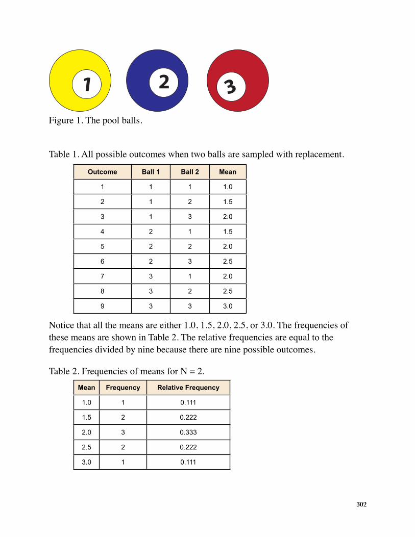
1 2 3Figure 1. The pool balls.

Table 1. All possible outcomes when two balls are sampled with replacement.

Outcome Ball 1 Ball 2 Mean

1 1 1 1.0

2 1 2 1.5

3 1 3 2.0

4 2 1 1.5

5 2 2 2.0

6 2 3 2.5

7 3 1 2.0

8 3 2 2.5

9 3 3 3.0

Notice that all the means are either 1.0, 1.5, 2.0, 2.5, or 3.0. The frequencies of these means are shown in Table 2. The relative frequencies are equal to the frequencies divided by nine because there are nine possible outcomes.

Table 2. Frequencies of means for N = 2.Mean Frequency Relative Frequency

1.0 1 0.111

1.5 2 0.222

2.0 3 0.333

2.5 2 0.222

3.0 1 0.111

302

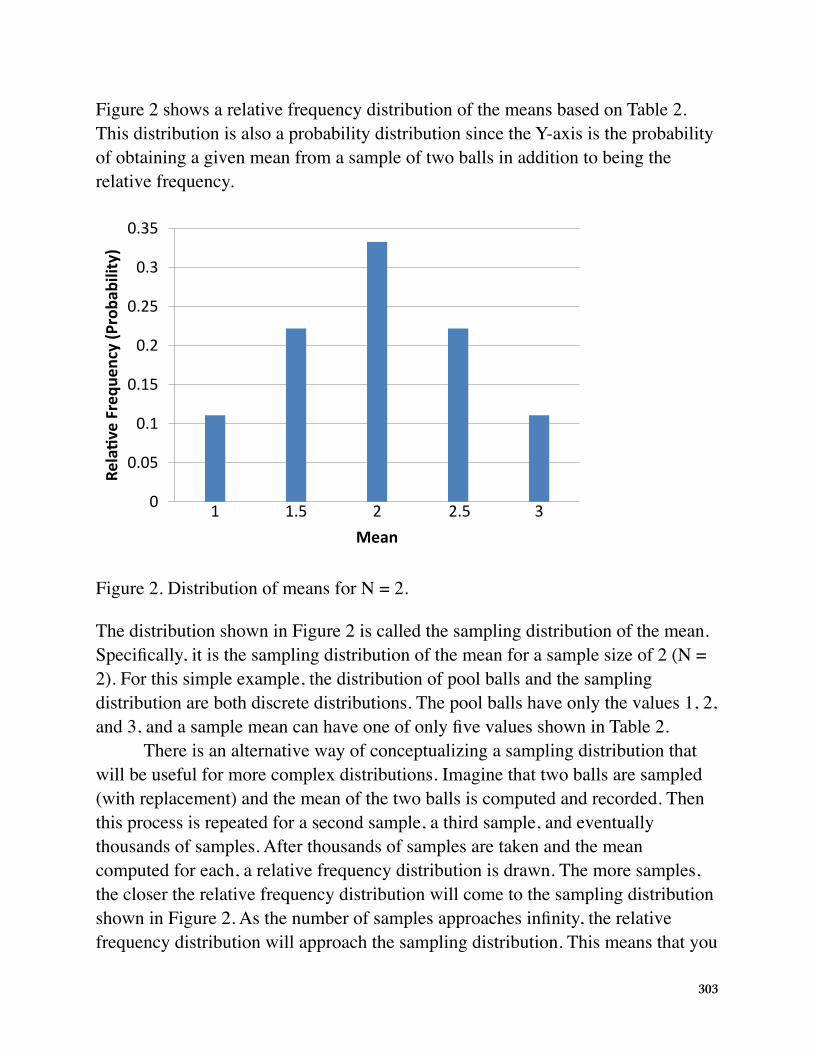
Figure 2 shows a relative frequency distribution of the means based on Table 2. This distribution is also a probability distribution since the Y-axis is the probability of obtaining a given mean from a sample of two balls in addition to being the relative frequency.

0

0.05

0.1

0.15

0.2

0.25

0.3

0.35

1 1.5 2 2.5 3

RelaƟ

ve F

requ

ency

(Pro

babi

lity)

Mean

Figure 2. Distribution of means for N = 2.

The distribution shown in Figure 2 is called the sampling distribution of the mean. Specifically, it is the sampling distribution of the mean for a sample size of 2 (N = 2). For this simple example, the distribution of pool balls and the sampling distribution are both discrete distributions. The pool balls have only the values 1, 2, and 3, and a sample mean can have one of only five values shown in Table 2.

There is an alternative way of conceptualizing a sampling distribution that will be useful for more complex distributions. Imagine that two balls are sampled (with replacement) and the mean of the two balls is computed and recorded. Then this process is repeated for a second sample, a third sample, and eventually thousands of samples. After thousands of samples are taken and the mean computed for each, a relative frequency distribution is drawn. The more samples, the closer the relative frequency distribution will come to the sampling distribution shown in Figure 2. As the number of samples approaches infinity, the relative frequency distribution will approach the sampling distribution. This means that you

303

can conceive of a sampling distribution as being a relative frequency distribution based on a very large number of samples. To be strictly correct, the relative frequency distribution approaches the sampling distribution as the number of samples approaches infinity.

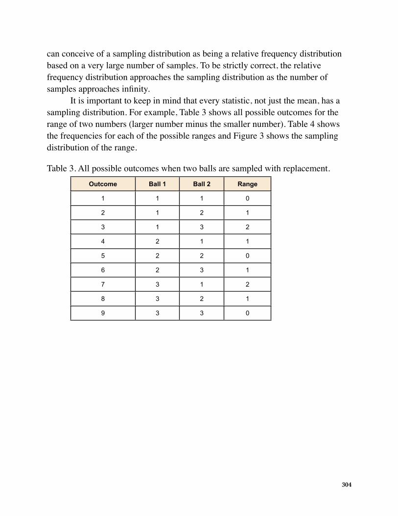
It is important to keep in mind that every statistic, not just the mean, has a sampling distribution. For example, Table 3 shows all possible outcomes for the range of two numbers (larger number minus the smaller number). Table 4 shows the frequencies for each of the possible ranges and Figure 3 shows the sampling distribution of the range.

Table 3. All possible outcomes when two balls are sampled with replacement.Outcome Ball 1 Ball 2 Range

1 1 1 0

2 1 2 1

3 1 3 2

4 2 1 1

5 2 2 0

6 2 3 1

7 3 1 2

8 3 2 1

9 3 3 0

304

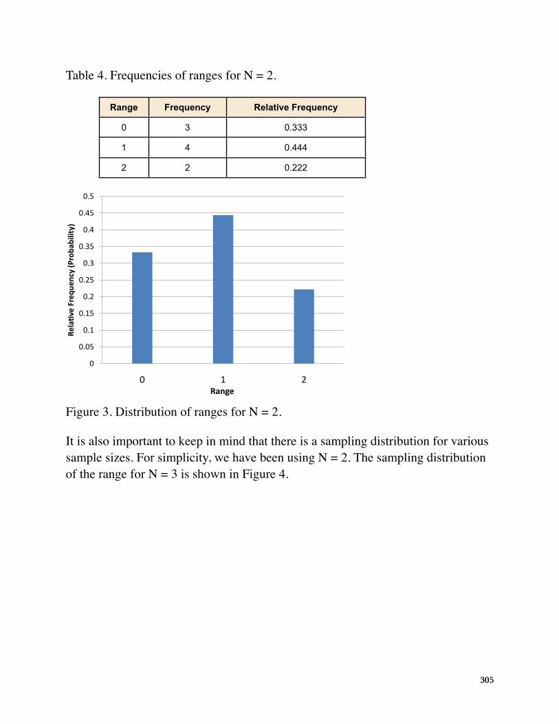
Table 4. Frequencies of ranges for N = 2.

Range Frequency Relative Frequency

0 3 0.333

1 4 0.444

2 2 0.222

0

0.05

0.1

0.15

0.2

0.25

0.3

0.35

0.4

0.45

0.5

0 1 2

Rela�ve&Frequ

ency&(P

roba

bility)

Range

Figure 3. Distribution of ranges for N = 2.

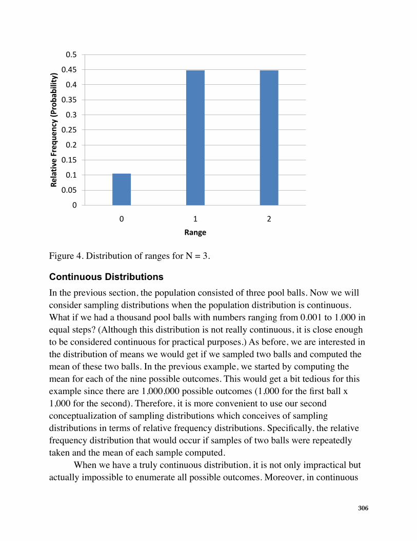
It is also important to keep in mind that there is a sampling distribution for various sample sizes. For simplicity, we have been using N = 2. The sampling distribution of the range for N = 3 is shown in Figure 4.

305

0

0.05

0.1

0.15

0.2

0.25

0.3

0.35

0.4

0.45

0.5

0 1 2

Relativ

e(Freq

uency((Proba

bility)

Range

Figure 4. Distribution of ranges for N = 3.

Continuous DistributionsIn the previous section, the population consisted of three pool balls. Now we will consider sampling distributions when the population distribution is continuous. What if we had a thousand pool balls with numbers ranging from 0.001 to 1.000 in equal steps? (Although this distribution is not really continuous, it is close enough to be considered continuous for practical purposes.) As before, we are interested in the distribution of means we would get if we sampled two balls and computed the mean of these two balls. In the previous example, we started by computing the mean for each of the nine possible outcomes. This would get a bit tedious for this example since there are 1,000,000 possible outcomes (1,000 for the first ball x 1,000 for the second). Therefore, it is more convenient to use our second conceptualization of sampling distributions which conceives of sampling distributions in terms of relative frequency distributions. Specifically, the relative frequency distribution that would occur if samples of two balls were repeatedly taken and the mean of each sample computed.

When we have a truly continuous distribution, it is not only impractical but actually impossible to enumerate all possible outcomes. Moreover, in continuous

306

distributions, the probability of obtaining any single value is zero. Therefore, as discussed in the section “Distributions” in Chapter 1, these values are called probability densities rather than probabilities.

Sampling Distributions and Inferential StatisticsAs we stated in the beginning of this chapter, sampling distributions are important for inferential statistics. In the examples given so far, a population was specified and the sampling distribution of the mean and the range were determined. In practice, the process proceeds the other way: you collect sample data, and from these data you estimate parameters of the sampling distribution. This knowledge of the sampling distribution can be very useful. For example, knowing the degree to which means from different samples would differ from each other and from the population mean would give you a sense of how close your particular sample mean is likely to be to the population mean. Fortunately, this information is directly available from a sampling distribution. The most common measure of how much sample means differ from each other is the standard deviation of the sampling distribution of the mean. This standard deviation is called the standard error of the mean. If all the sample means were very close to the population mean, then the standard error of the mean would be small. On the other hand, if the sample means varied considerably, then the standard error of the mean would be large.

To be specific, assume your sample mean were 125 and you estimated that the standard error of the mean were 5 (using a method shown in a later section). If you had a normal distribution, then it would be likely that your sample mean would be within 10 units of the population mean since most of a normal distribution is within two standard deviations of the mean.

Keep in mind that all statistics have sampling distributions, not just the mean. In later sections we will be discussing the sampling distribution of the variance, the sampling distribution of the difference between means, and the sampling distribution of Pearson's correlation, among others.

307

Sampling Distribution of the Meanby David M. Lane

Prerequisites• Chapter 3: Variance Sum Law I • Chapter 9: Introduction to Sampling Distributions

Learning Objectives1. State the mean and variance of the sampling distribution of the mean2. Compute the standard error of the mean3. State the central limit theoremThe sampling distribution of the mean was defined in the section introducing sampling distributions. This section reviews some important properties of the sampling distribution of the mean.

MeanThe mean of the sampling distribution of the mean is the mean of the population from which the scores were sampled. Therefore, if a population has a mean μ, then the mean of the sampling distribution of the mean is also μ. The symbol μM is used to refer to the mean of the sampling distribution of the mean. Therefore, the formula for the mean of the sampling distribution of the mean can be written as:

µM = µ

VarianceThe variance of the sampling distribution of the mean is computed as follows:Sampling Distribution of the Mean

ଶߪ =ଶߪ

ߪ =ߪξ

Sampling Distribution of difference between means

ெభெమߤ = ଵߤ െ ଶߤ

ெభெమߪଶ = ெభߪ

ଶ െ ெమߪଶ

ெଶߪ =ଶߪ

ெభெమߪ = ඨߪଵଶ

ଵ+ଶଶߪ

ଶ

That is, the variance of the sampling distribution of the mean is the population variance divided by N, the sample size (the number of scores used to compute a mean). Thus, the larger the sample size, the smaller the variance of the sampling distribution of the mean.(optional paragraph) This expression can be derived very easily from the variance sum law. Let's begin by computing the variance of the sampling distribution of the

308

sum of three numbers sampled from a population with variance σ2. The variance of the sum would be σ2 + σ2 + σ2. For N numbers, the variance would be Nσ2. Since the mean is 1/N times the sum, the variance of the sampling distribution of the mean would be 1/N2 times the variance of the sum, which equals σ2/N.

The standard error of the mean is the standard deviation of the sampling distribution of the mean. It is therefore the square root of the variance of the sampling distribution of the mean and can be written as:

Sampling Distribution of the Mean

ଶߪ =ଶߪ

ߪ =ߪξ

Sampling Distribution of difference between means

ெభெమߤ = ଵߤ െ ଶߤ

ெభெమߪଶ = ெభߪ

ଶ െ ெమߪଶ

ெଶߪ =ଶߪ

ெభெమߪ = ඨߪଵଶ

ଵ+ଶଶߪ

ଶ

The standard error is represented by a σ because it is a standard deviation. The subscript (M) indicates that the standard error in question is the standard error of the mean.

Central Limit TheoremThe central limit theorem states that:

Given a population with a finite mean µ and a finite non-zero variance σ2, the sampling distribution of the mean approaches a normal distribution with a mean of µ and a variance of σ2/N as N, the sample size, increases.

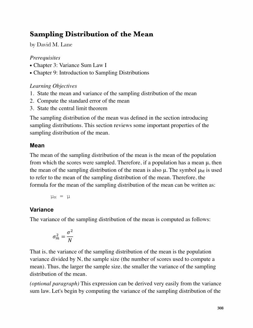
The expressions for the mean and variance of the sampling distribution of the mean are not new or remarkable. What is remarkable is that regardless of the shape of the parent population, the sampling distribution of the mean approaches a normal distribution as N increases. If you have used the “Central Limit Theorem Demo,” (external link; requires Java) you have already seen this for yourself. As a reminder, Figure 1 shows the results of the simulation for N = 2 and N = 10. The parent population was a uniform distribution. You can see that the distribution for N = 2 is far from a normal distribution. Nonetheless, it does show that the scores are denser in the middle than in the tails. For N = 10 the distribution is quite close to a normal distribution. Notice that the means of the two distributions are the same, but that the spread of the distribution for N = 10 is smaller.

309

11/8/10 12:43 PMSampling Distribution of the Mean

Page 3 of 4http://onlinestatbook.com/2/sampling_distributions/samp_dist_mean.html

Figure 2 shows how closely the sampling distribution of the mean approximates anormal distribution even when the parent population is very non-normal. If you lookclosely you can see that the sampling distributions do have a slight positive skew. Thelarger the sample size, the closer the sampling distribution of the mean would be to anormal distribution.

Figure 2. A simulation of a samplingdistribution. The parent population is verynon-normal.

Check Answer Previous Question Next Question

Figure 1. A simulation of a sampling distribution. The parent population is uniform. The blue line under “16” indicates that 16 is the mean. The red line extends from the mean plus and minus one standard deviation.

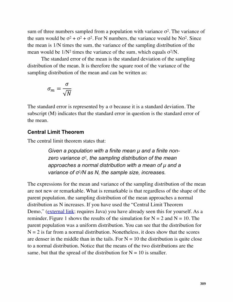
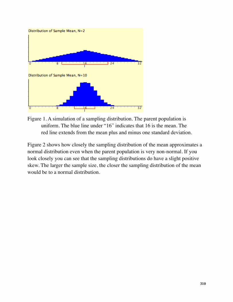
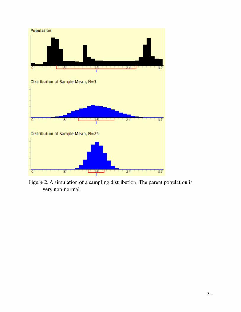
Figure 2 shows how closely the sampling distribution of the mean approximates a normal distribution even when the parent population is very non-normal. If you look closely you can see that the sampling distributions do have a slight positive skew. The larger the sample size, the closer the sampling distribution of the mean would be to a normal distribution.

310

11/8/10 12:43 PMSampling Distribution of the Mean

Page 3 of 4http://onlinestatbook.com/2/sampling_distributions/samp_dist_mean.html

Figure 2 shows how closely the sampling distribution of the mean approximates anormal distribution even when the parent population is very non-normal. If you lookclosely you can see that the sampling distributions do have a slight positive skew. Thelarger the sample size, the closer the sampling distribution of the mean would be to anormal distribution.

Figure 2. A simulation of a samplingdistribution. The parent population is verynon-normal.

Check Answer Previous Question Next Question

Figure 2. A simulation of a sampling distribution. The parent population is very non-normal.

311

Sampling Distribution of Difference Between Meansby David M. Lane

Prerequisites• Chapter 3: Variance Sum Law I • Chapter 9: Sampling Distributions• Chapter 9: Sampling Distribution of the Mean

Learning Objectives1. State the mean and variance of the sampling distribution of the difference

between means2. Compute the standard error of the difference between means3. Compute the probability of a difference between means being above a specified

valueStatistical analyses are very often concerned with the difference between means. A typical example is an experiment designed to compare the mean of a control group with the mean of an experimental group. Inferential statistics used in the analysis of this type of experiment depend on the sampling distribution of the difference between means.

The sampling distribution of the difference between means can be thought of as the distribution that would result if we repeated the following three steps over and over again: (1) sample n1 scores from Population 1 and n2 scores from Population 2, (2) compute the means of the two samples (M1 and M2), and (3) compute the difference between means, M1 - M2. The distribution of the differences between means is the sampling distribution of the difference between means.

As you might expect, the mean of the sampling distribution of the difference between means is:

Sampling Distribution of the Mean

�� =��

�

� =���

Sampling Distribution of difference between means

���� = �� ��

����� = ��

� ���

�� =��

�

���� = ����

��+���

��

which says that the mean of the distribution of differences between sample means is equal to the difference between population means. For example, say that the mean test score of all 12-year-olds in a population is 34 and the mean of 10-year-olds is 25. If numerous samples were taken from each age group and the mean

312

difference computed each time, the mean of these numerous differences between sample means would be 34 - 25 = 9.

From the variance sum law, we know that:

which says that the variance of the sampling distribution of the difference between means is equal to the variance of the sampling distribution of the mean for Population 1 plus the variance of the sampling distribution of the mean for Population 2. Recall the formula for the variance of the sampling distribution of the mean:

Sampling Distribution of the Mean

�� =��

�

� =���

Sampling Distribution of difference between means

���� = �� ��

����� = ��

� ���

�� =��

�

���� = ����

��+���

��

Since we have two populations and two samples sizes, we need to distinguish between the two variances and sample sizes. We do this by using the subscripts 1 and 2. Using this convention, we can write the formula for the variance of the sampling distribution of the difference between means as:

Since the standard error of a sampling distribution is the standard deviation of the sampling distribution, the standard error of the difference between means is:

Just to review the notation, the symbol on the left contains a sigma (σ), which means it is a standard deviation. The subscripts M1 - M2 indicate that it is the standard deviation of the sampling distribution of M1 - M2.

Now let's look at an application of this formula. Assume there are two species of green beings on Mars. The mean height of Species 1 is 32 while the mean height of Species 2 is 22. The variances of the two species are 60 and 70,

313

respectively, and the heights of both species are normally distributed. You randomly sample 10 members of Species 1 and 14 members of Species 2. What is the probability that the mean of the 10 members of Species 1 will exceed the mean of the 14 members of Species 2 by 5 or more? Without doing any calculations, you probably know that the probability is pretty high since the difference in population means is 10. But what exactly is the probability?

First, let’s determine the sampling distribution of the difference between means. Using the formulas above, the mean is

����� = 32 22 = 10

����� = �6010 +

7014 = 3.317

����� = ����

��+���

��= ��

�

� +��

� = �2��

�

����� = �2��

� = �(2)(64)8 = 4

Sampling Distribution of Pearson’s r

The standard error is:

����� = 32 22 = 10

����� = �6010 +

7014 = 3.317

����� = ����

��+���

��= ��

�

� +��

� = �2��

�

����� = �2��

� = �(2)(64)8 = 4

Sampling Distribution of Pearson’s r

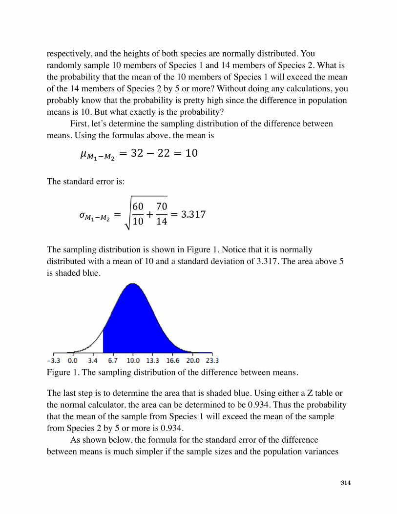
The sampling distribution is shown in Figure 1. Notice that it is normally distributed with a mean of 10 and a standard deviation of 3.317. The area above 5 is shaded blue.

11/8/10 1:08 PMSampling Distribution of Difference Between Means

Page 3 of 4http://onlinestatbook.com/2/sampling_distributions/samplingdist_diff_means.html

The sampling distribution is shown in Figure 1. Notice that it is normally distributed witha mean of 10 and a standard deviation of 3.317. The area above 5 is shaded blue.

Figure 1. The sampling distributionof the difference between means.

The last step is to determine the area that is shaded blue. Using either a Z table or thenormal calculator, the area can be determined to be 0.934. Thus the probability thatthe mean of the sample from Species 2 will exceed the mean of the sample fromSpecies 1 by 5 or more is 0.934.

As shown below, the formula for the standard error of the difference betweenmeans is much simpler if the sample sizes and the population variances are equal. Sincethe variances and samples sizes are the same, there is no need to use the subscripts 1and 2 to differentiate these terms.

This simplified version of the formula can be used for the following problem: The meanheight of 15-year olds boys (in cm) is 175 and the variance is 64. For girls, the mean is165 and the variance is 64. If eight boys and eight girls were sampled, what is theprobability that the mean height of the sample of girls would be higher than the meanheight of the boys? In other words, what is the probability that the mean height of girlsminus the mean height of boys is greater than 0?

As before, the problem can be solved in terms of the sampling distribution of thedifference between means (girls - boys). The mean of the distribution is 165 - 175 = -10. The standard deviation of the distribution is:

A graph of the distribution is shown in Figure 2. It is clear that it is unlikely that the

Figure 1. The sampling distribution of the difference between means.

The last step is to determine the area that is shaded blue. Using either a Z table or the normal calculator, the area can be determined to be 0.934. Thus the probability that the mean of the sample from Species 1 will exceed the mean of the sample from Species 2 by 5 or more is 0.934.

As shown below, the formula for the standard error of the difference between means is much simpler if the sample sizes and the population variances

314

are equal. When the variances and samples sizes are the same, there is no need to use the subscripts 1 and 2 to differentiate these terms.

����� = 32 22 = 10

����� = �6010 +

7014 = 3.317

����� = ����

��+���

��= ��

�

� +��

� = �2��

�

����� = �2��

� = �(2)(64)8 = 4

Sampling Distribution of Pearson’s r

This simplified version of the formula can be used for the following problem: The mean height of 15-year-old boys (in cm) is 175 and the variance is 64. For girls, the mean is 165 and the variance is 64. If eight boys and eight girls were sampled, what is the probability that the mean height of the sample of girls would be higher than the mean height of the sample of boys? In other words, what is the probability that the mean height of girls minus the mean height of boys is greater than 0?

As before, the problem can be solved in terms of the sampling distribution of the difference between means (girls - boys). The mean of the distribution is 165 - 175 = -10. The standard deviation of the distribution is:

����� = 32 22 = 10

����� = �6010 +

7014 = 3.317

����� = ����

��+���

��= ��

�

� +��

� = �2��

�

����� = �2��

� = �(2)(64)8 = 4

Sampling Distribution of Pearson’s r

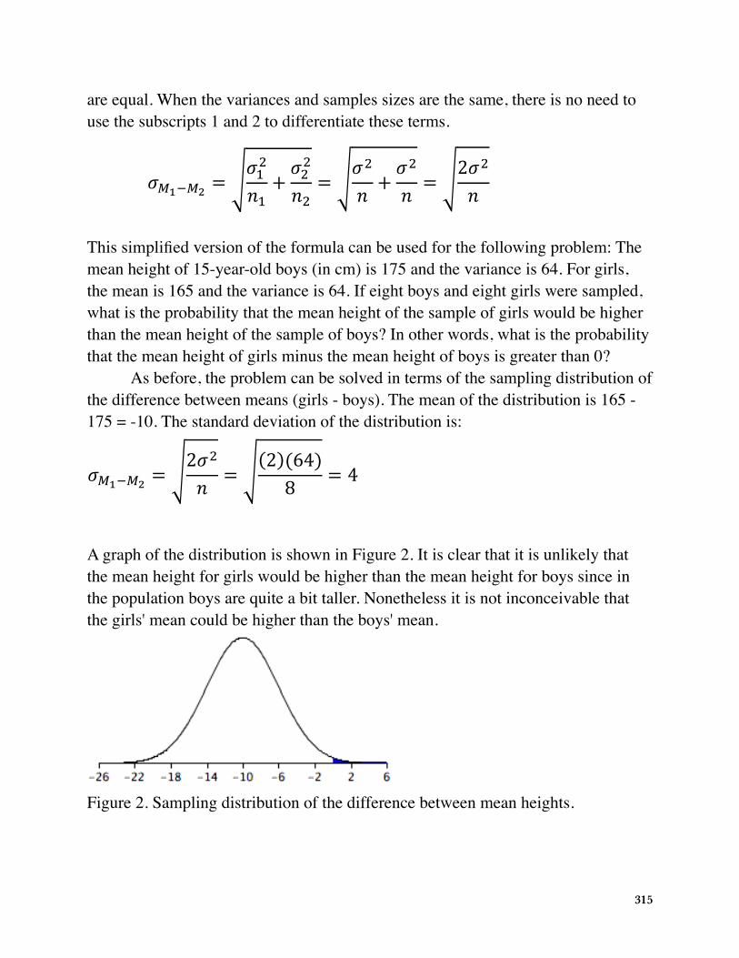
A graph of the distribution is shown in Figure 2. It is clear that it is unlikely that the mean height for girls would be higher than the mean height for boys since in the population boys are quite a bit taller. Nonetheless it is not inconceivable that the girls' mean could be higher than the boys' mean.

11/8/10 1:08 PMSampling Distribution of Difference Between Means

Page 4 of 4http://onlinestatbook.com/2/sampling_distributions/samplingdist_diff_means.html

mean height for girls would be higher than the mean height for boys since in thepopulation boys are quite a bit taller. Nonetheless it is not inconceivable that the girls'mean could be higher than the boys' mean.

Figure 2. Sampling distribution ofthe difference between meanheights.

A difference between means of 0 or higher is a difference of 10/4 = 2.5 standarddeviations above the mean of -10. The probability of a score 2.5 or more standarddeviations above the mean is 0.0062.

Check Answer Previous Question Next Question

Question 1 out of 4.Population 1 has a mean of 20 and a variance of 100. Population 2 has a meanof 15 and a variance of 64. You sample 20 scores from Pop 1 and 16 scoresfrom Pop 2. What is the mean of the sampling distribution of the differencebetween means (Pop 1 - Pop 2)?

Previous Section | Next Section

Figure 2. Sampling distribution of the difference between mean heights.

315

A difference between means of 0 or higher is a difference of 10/4 = 2.5 standard deviations above the mean of -10. The probability of a score 2.5 or more standard deviations above the mean is 0.0062.

316

Sampling Distribution of Pearson's rby David M. Lane

Prerequisites• Chapter 4: Values of the Pearson Correlation• Chapter 9: Introduction to Sampling Distributions

Learning Objectives1. State how the shape of the sampling distribution of r deviates from normality2. Transform r to z'3. Compute the standard error of z'4. Calculate the probability of obtaining an r above a specified valueAssume that the correlation between quantitative and verbal SAT scores in a given population is 0.60. In other words, ρ = 0.60. If 12 students were sampled randomly, the sample correlation, r, would not be exactly equal to 0.60. Naturally different samples of 12 students would yield different values of r. The distribution of values of r after repeated samples of 12 students is the sampling distribution of r.

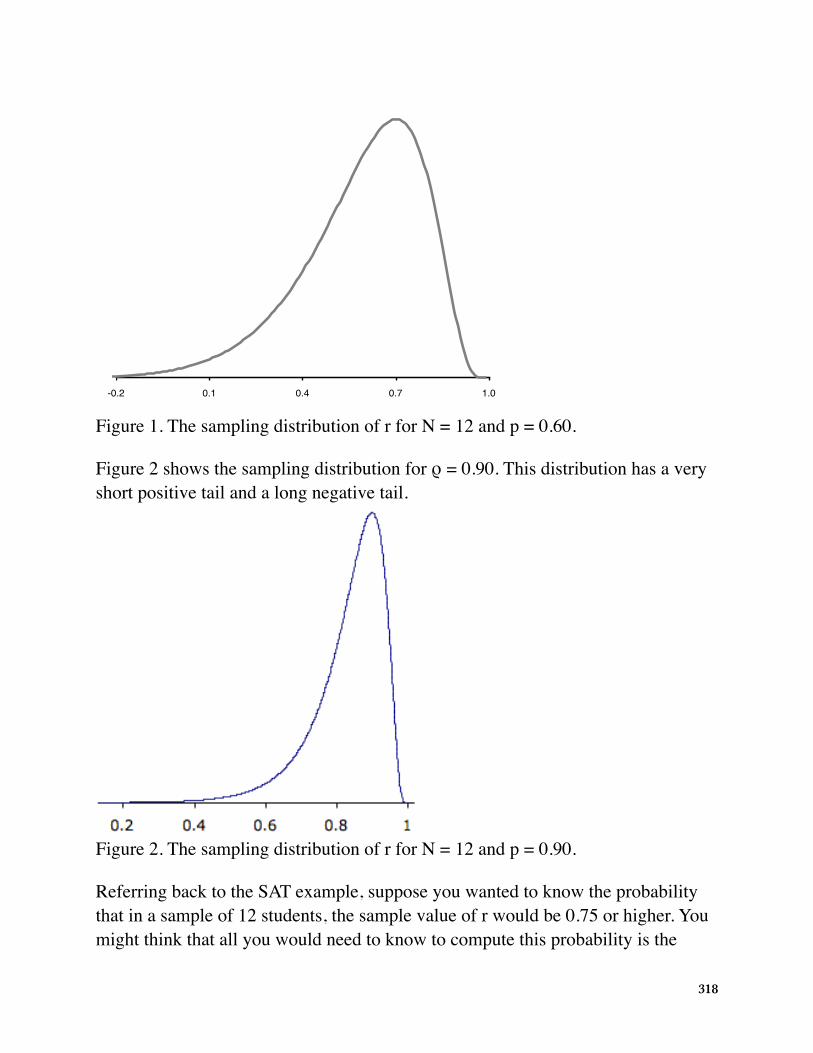
The shape of the sampling distribution of r for the above example is shown in Figure 1. You can see that the sampling distribution is not symmetric: it is negatively skewed. The reason for the skew is that r cannot take on values greater than 1.0 and therefore the distribution cannot extend as far in the positive direction as it can in the negative direction. The greater the value of ρ, the more pronounced the skew.

317

-0.2 0.1 0.4 0.7 1.0

Figure 1. The sampling distribution of r for N = 12 and p = 0.60.

Figure 2 shows the sampling distribution for ρ = 0.90. This distribution has a very short positive tail and a long negative tail.

11/8/10 1:18 PMSampling Distribution of Pearson's r

Page 2 of 3http://onlinestatbook.com/2/sampling_distributions/samp_dist_r.html

Figure 2 shows the sampling distribution for ρ = 0.90. This distribution has a very shortpositive tail and a long negative tail.

Figure 2. The sampling distributionof r for N = 12 and ρ = 0.90.

Referring back to the SAT example, suppose you wanted to know the probabilitythat in a sample of 19 students, the sample value of r would be 0.75 or higher. Youmight think that all you would need to know to compute this probability is the meanand standard error of the sampling distribution of r. However, since the samplingdistribution is not normal, you would still not be able to solve the problem. Fortunately,the statistician Fisher developed a way to transform r to a variable that is normallydistributed with a known standard error. The variable is called z' and the formula for thetransformation is given below.

z' = 0.5 ln[(1+r)/(1-r)]

The details of the formula are not important here since normally you will use either atable or calculator to do the transformation. What is important is that z' is normallydistributed and has a standard error of

where N is the number of pairs of scores.Let's return to the question of determining the probability of getting a sample

correlation of 0.75 or above in a sample of 12 from a population with a correlation of0.60. The first step is to convert both 0.60 and 0.75 to z's. The values are 0.693 and0.973 respectively. The standard error of z' for N = 12 is 0.333. Therefore thequestion is reduced to the following: given a normal distribution with a mean of 0.693and a standard deviation of 0.333, what is the probability of obtaining a value of 0.973

Figure 2. The sampling distribution of r for N = 12 and p = 0.90.

Referring back to the SAT example, suppose you wanted to know the probability that in a sample of 12 students, the sample value of r would be 0.75 or higher. You might think that all you would need to know to compute this probability is the

318

mean and standard error of the sampling distribution of r. However, since the sampling distribution is not normal, you would still not be able to solve the problem. Fortunately, the statistician Fisher developed a way to transform r to a variable that is normally distributed with a known standard error. The variable is called z' and the formula for the transformation is given below.

z' = 0.5 ln[(1+r)/(1-r)]

The details of the formula are not important here since normally you will use either a table or calculator (external link) to do the transformation. What is important is that z' is normally distributed and has a standard error of

1�� � 3

Sampling Distribution of a Proportion

���(1� �)

�� =���(1 � �)

� = ��(1 � �)�

�� = �0.60(1 � .60)10 = 0.155

where N is the number of pairs of scores.Let's return to the question of determining the probability of getting a sample

correlation of 0.75 or above in a sample of 12 from a population with a correlation of 0.60. The first step is to convert both 0.60 and 0.75 to their z' values, which are 0.693 and 0.973, respectively. The standard error of z' for N = 12 is 0.333. Therefore, the question is reduced to the following: given a normal distribution with a mean of 0.693 and a standard deviation of 0.333, what is the probability of obtaining a value of 0.973 or higher? The answer can be found directly from the normal calculator (external link) to be 0.20. Alternatively, you could use the formula:

z = (X - µ)/σ = (0.973 - 0.693)/0.333 = 0.841

and use a table to find that the area above 0.841 is 0.20.

319

Sampling Distribution of pby David M. Lane

Prerequisites• Chapter 5: Binomial Distribution• Chapter 7: Normal Approximation to the Binomial• Chapter 9: Introduction to Sampling Distributions

Learning Objectives1. Compute the mean and standard deviation of the sampling distribution of p2. State the relationship between the sampling distribution of p and the normal

distributionAssume that in an election race between Candidate A and Candidate B, 0.60

of the voters prefer Candidate A. If a random sample of 10 voters were polled, it is unlikely that exactly 60% of them (6) would prefer Candidate A. By chance the proportion in the sample preferring Candidate A could easily be a little lower than 0.60 or a little higher than 0.60. The sampling distribution of p is the distribution that would result if you repeatedly sampled 10 voters and determined the proportion (p) that favored Candidate A.

The sampling distribution of p is a special case of the sampling distribution of the mean. Table 1 shows a hypothetical random sample of 10 voters. Those who prefer Candidate A are given scores of 1 and those who prefer Candidate B are given scores of 0. Note that seven of the voters prefer candidate A so the sample proportion (p) is

p = 7/10 = 0.70

As you can see, p is the mean of the 10 preference scores.

320

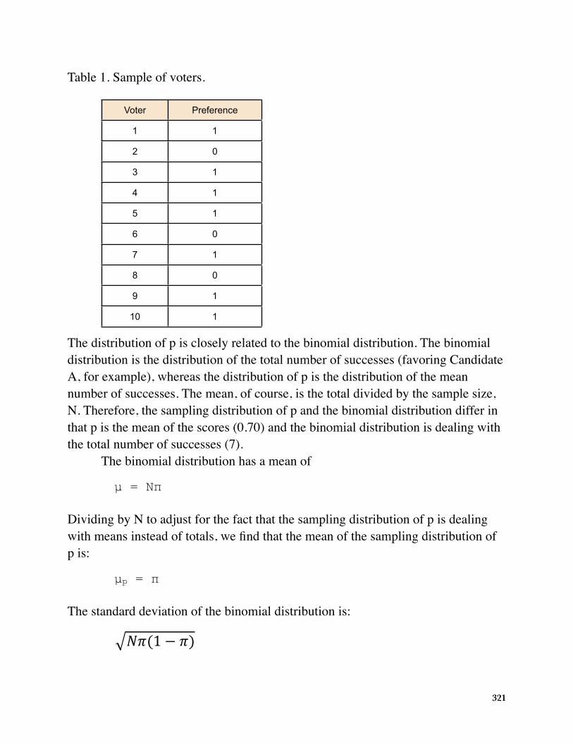
Table 1. Sample of voters.

Voter Preference

1 1

2 0

3 1

4 1

5 1

6 0

7 1

8 0

9 1

10 1

The distribution of p is closely related to the binomial distribution. The binomial distribution is the distribution of the total number of successes (favoring Candidate A, for example), whereas the distribution of p is the distribution of the mean number of successes. The mean, of course, is the total divided by the sample size, N. Therefore, the sampling distribution of p and the binomial distribution differ in that p is the mean of the scores (0.70) and the binomial distribution is dealing with the total number of successes (7).

The binomial distribution has a mean of

µ = Nπ

Dividing by N to adjust for the fact that the sampling distribution of p is dealing with means instead of totals, we find that the mean of the sampling distribution of p is:

µp = π

The standard deviation of the binomial distribution is:

1�� � 3

Sampling Distribution of a Proportion

���(1� �)

�� =���(1 � �)

� = ��(1 � �)�

�� = �0.60(1 � .60)10 = 0.155

321

Dividing by N because p is a mean not a total, we find the standard error of p:

1�� � 3

Sampling Distribution of a Proportion

���(1� �)

�� =���(1 � �)

� = ��(1 � �)�

�� = �0.60(1 � .60)10 = 0.155

Returning to the voter example, π = 0.60 (Don't confuse π = 0.60, the population proportion, with p = 0.70, the sample proportion) and N = 10. Therefore, the mean of the sampling distribution of p is 0.60. The standard error is

1�� � 3

Sampling Distribution of a Proportion

���(1� �)

�� =���(1 � �)

� = ��(1 � �)�

�� = �0.60(1 � .60)10 = 0.155

The sampling distribution of p is a discrete rather than a continuous distribution. For example, with an N of 10, it is possible to have a p of 0.50 or a p of 0.60, but not a p of 0.55.

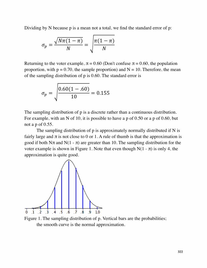
The sampling distribution of p is approximately normally distributed if N is fairly large and π is not close to 0 or 1. A rule of thumb is that the approximation is good if both Nπ and N(1 - π) are greater than 10. The sampling distribution for the voter example is shown in Figure 1. Note that even though N(1 - π) is only 4, the approximation is quite good.

11/8/10 1:36 PMSampling Distribution of a proportion

Page 3 of 3http://onlinestatbook.com/2/sampling_distributions/samp_dist_p.html

The sampling distribution of p is approximately normally distributed if N is fairlylarge and π is not close to 0 or 1. A rule of thumb is that the approximation isgood if both N π and N(1 - π) are both greater than 10. The sampling distributionfor the voter example is shown in Figure 1. Note that even though N(1 - π) is only4, the approximation is quite good.

Figure 1. The sampling distribution of p.Vertical bars are the probabilities; the smoothcurve is the normal approximation.

Check Answer Previous Question Next Question

Question 1 out of 4.The binomial distribution is the distribution of the total number ofsuccesses whereas the distribution of p is:

the distribution of the mean number of successes

the distribution of the total number of failures

the distribution of the ratio of successes to failures

a distribution with a mean of .5

Previous Section | Next Section

Figure 1. The sampling distribution of p. Vertical bars are the probabilities; the smooth curve is the normal approximation.

322

Statistical Literacyby David M. Lane

Prerequisites• Chapter 9: Introduction• Chapter 9: Sampling Distribution of the Mean

The monthly jobs report always gets a lot of attention. Presidential candidates refer to the report when it favors their position. Referring to the August 2012 report in which only 96,000 jobs were created, Republican presidential challenger Mitt Romney stated "the weak jobs report is devastating news for American workers and American families ... a harsh indictment of the president's handling of the economy." When the September 2012 report was released showing 114,000 jobs were created (and the previous report was revised upwards), some supporters of Romney claimed the data were tampered with for political reasons. The most famous statement, "Unbelievable jobs numbers...these Chicago guys will do anything..can't debate so change numbers," was made by former Chairman and CEO of General Electric.

What do you think?The standard error of the monthly estimate is 100,000. Given that, what do you think of the difference between the two job reports?

The difference between the two reports is very small given that the standard error is 100,000. It is not sensible to take any single jobs report too seriously.

323

Exercises

PrerequisitesAll material presented in the Sampling Distributions chapter

1. A population has a mean of 50 and a standard deviation of 6. (a) What are the mean and standard deviation of the sampling distribution of the mean for N = 16? (b) What are the mean and standard deviation of the sampling distribution of the mean for N = 20?

2. Given a test that is normally distributed with a mean of 100 and a standard deviation of 12, find:a. the probability that a single score drawn at random will be greater than 110b. the probability that a sample of 25 scores will have a mean greater than 105c. the probability that a sample of 64 scores will have a mean greater than 105d. the probability that the mean of a sample of 16 scores will be either less than 95 or greater than 105

3. What term refers to the standard deviation of a sampling distribution?

4. (a) If the standard error of the mean is 10 for N = 12, what is the standard error of the mean for N = 22? (b) If the standard error of the mean is 50 for N = 25, what is it for N = 64?

5. A questionnaire is developed to assess women’s and men’s attitudes toward using animals in research. One question asks whether animal research is wrong and is answered on a 7-point scale. Assume that in the population, the mean for women is 5, the mean for men is 4, and the standard deviation for both groups is 1.5. Assume the scores are normally distributed. If 12 women and 12 men are selected randomly, what is the probability that the mean of the women will be more than 2 points higher than the mean of the men?

6. If the correlation between reading achievement and math achievement in the population of fifth graders were 0.60, what would be the probability that in a sample of 28 students, the sample correlation coefficient would be greater than 0.65?

324

7. If numerous samples of N = 15 are taken from a uniform distribution and a relative frequency distribution of the means is drawn, what would be the shape of the frequency distribution?

8. A normal distribution has a mean of 20 and a standard deviation of 10. Two scores are sampled randomly from the distribution and the second score is subtracted from the first. What is the probability that the difference score will be greater than 5? Hint: Read the Variance Sum Law section of Chapter 3.

9. What is the shape of the sampling distribution of r? In what way does the shape depend on the size of the population correlation?

10. If you sample one number from a standard normal distribution, what is the probability it will be 0.5?

11. A variable is normally distributed with a mean of 120 and a standard deviation of 5. Four scores are randomly sampled. What is the probability that the mean of the four scores is above 127?

12. The correlation between self-esteem and extraversion is .30. A sample of 84 is taken. a. What is the probability that the correlation will be less than 0.10? b. What is the probability that the correlation will be greater than 0.25?

13. The mean GPA for students in School A is 3.0; the mean GPA for students in School B is 2.8. The standard deviation in both schools is 0.25. The GPAs of both schools are normally distributed. If 9 students are randomly sampled from each school, what is the probability that:a. the sample mean for School A will exceed that of School B by 0.5 or more?b. the sample mean for School B will be greater than the sample mean for School A?

14. In a city, 70% of the people prefer Candidate A. Suppose 30 people from this city were sampled.a. What is the mean of the sampling distribution of p? b. What is the standard error of p?

325

c. What is the probability that 80% or more of this sample will prefer Candidate A?

15. When solving problems where you need the sampling distribution of r, what is the reason for converting from r to z’?

16. In the population, the mean SAT score is 1000. Would you be more likely (or equally likely) to get a sample mean of 1200 if you randomly sampled 10 students or if you randomly sampled 30 students? Explain.

17. True/false: The standard error of the mean is smaller when N = 20 than when N = 10.

18. True/false: The sampling distribution of r = .8 becomes normal as N increases.

19. True/false: You choose 20 students from the population and calculate the mean of their test scores. You repeat this process 100 times and plot the distribution of the means. In this case, the sample size is 100.

20. True/false: In your school, 40% of students watch TV at night. You randomly ask 5 students every day if they watch TV at night. Every day, you would find that 2 of the 5 do watch TV at night.

21. True/false: The median has a sampling distribution.

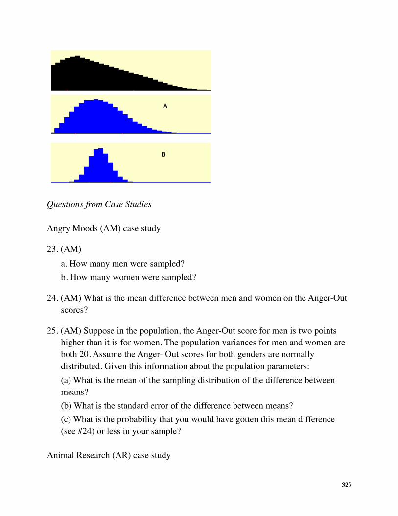
22. True/false: Refer to the figure below. The population distribution is shown in black, and its corresponding sampling distribution of the mean for N = 10 is labeled “A.”

326

���������� �������������

���������������������������

12*�,��- *���$�� �%�����$����� �����'��*���$�� �%�$�����$����� �����'�

13*�,��-��� ����������� ���������������$�������� ���$�����������������+�"��������'�

14*�,��-�"����������������"� ���(����������+�"��������������������$������������������ ������������$����*��������"� ����# �� ������������� ���$����� ��������10*����"������������+�"�������������������������� ������� ��%��������"���*���#�������������� ���� ��"���������"� ����� � ������)�, -��� ����������� ���������� ��������������"������������������������$������ ��'�,�-��� ����������� �� �����������������������������$������ ��',�-��� ������������� �����%��� ��%�"�$�"���� #����!���������� ������������,����.12-����

��������%�"��� ����'

��� ���������������������������

14*,�-���$�� �%��������$����� �����������#�������������������� ��� ������ ���'

15*�,�-��� ��������������� ������������� ��������$����������������� �� ��� ������ �������$����� ������������ �� ��� ������ ������������� �%'�,��*�2*�-

Questions from Case Studies

Angry Moods (AM) case study

23. (AM) a. How many men were sampled? b. How many women were sampled?

24. (AM) What is the mean difference between men and women on the Anger-Out scores?

25. (AM) Suppose in the population, the Anger-Out score for men is two points higher than it is for women. The population variances for men and women are both 20. Assume the Anger- Out scores for both genders are normally distributed. Given this information about the population parameters:(a) What is the mean of the sampling distribution of the difference between means?(b) What is the standard error of the difference between means?(c) What is the probability that you would have gotten this mean difference (see #24) or less in your sample?

Animal Research (AR) case study

327

26. (AR) How many people were sampled to give their opinions on animal research?

27. (AR) What is the correlation in this sample between the belief that animal research is wrong and belief that animal research is necessary?

28. (AR) Suppose the correlation between the belief that animal research is wrong and the belief that animal research is necessary is -.68 in the population.(a) Convert -.68 to z’.(b) Find the standard error of this sampling distribution.(c) Assuming the data used in this study was randomly sampled, what is the probability that you would get this correlation or stronger (closer to -1)?

328