9. Modular networks, motor control, and reinforcement learning · PDF file ·...
33
1 9. Modular networks, motor control, and reinforcement learning Lecture Notes on Brain and Computation Byoung-Tak Zhang Biointelligence Laboratory School of Computer Science and Engineering Graduate Programs in Cognitive Science, Brain Science and Bioinformatics Brain-Mind-Behavior Concentration Program Seoul National University E-mail: [email protected] This material is available online at http://bi.snu.ac.kr/ Fundamentals of Computational Neuroscience (The 2 nd Ed.), T. P. Trappenberg, 2010.
Transcript of 9. Modular networks, motor control, and reinforcement learning · PDF file ·...

1
9. Modular networks, motor control,
and reinforcement learning
Lecture Notes on Brain and Computation
Byoung-Tak Zhang
Biointelligence Laboratory
School of Computer Science and Engineering
Graduate Programs in Cognitive Science, Brain Science and Bioinformatics
Brain-Mind-Behavior Concentration Program
Seoul National University
E-mail: [email protected]
This material is available online at http://bi.snu.ac.kr/
Fundamentals of Computational Neuroscience (The 2nd Ed.), T. P. Trappenberg, 2010.

(C) 2010 SNU CSE Biointelligence Lab, http://bi.snu.ac.kr
Outline
2
9.1
9.2
9.3
9.4
9.5
9.6
Modular mapping networks
Coupled attractor networks
Sequence learning
Complementary memory systems
Motor learning and control
Reinforcement learning

(C) 2010 SNU CSE Biointelligence Lab, http://bi.snu.ac.kr
9.1 Modular mapping networks
Modular networks
Large-scale networks with constraints
Modular specialization in brain
Mixture of experts
Combining feedforward mapping networks
Experts: working modules
3

(C) 2010 SNU CSE Biointelligence Lab, http://bi.snu.ac.kr
9.1 Modular mapping networks
Mixture of experts (cont’d)
Property: - Universal function approximator → can solve any mapping task - ex) abstract function (Fig. 9.2)
Divide and conquer strategy
Training networks
Assign the experts to particular tasks
Train each expert on the designated task
Train the gating network (Credit-assignment problem)
Not appropriate in biology systems
4

(C) 2010 SNU CSE Biointelligence Lab, http://bi.snu.ac.kr
9.1 Modular mapping networks
The ‘what-and-where’ task
Two visual pathways
Ventral visual pathway (what)
Dorsal visual pathway (where)
Modular networks
What → object recognition (what)
Where → location of objects (where)
5

(C) 2010 SNU CSE Biointelligence Lab, http://bi.snu.ac.kr
9.1 Modular mapping networks
The ‘what-and-where’ task
Jacob’s idea (1991)
Input channels (26): retinal (25) & the task specification (1)
Output channels (18): objects (9) & location (9)
A single network with 36 hidden nodes using back-
propagation
Conflicting training
information
Temporal cross-talk
Spatial cross-talk
Task decomposition
6

(C) 2010 SNU CSE Biointelligence Lab, http://bi.snu.ac.kr
9.1 Modular mapping networks
Modular network for what-and-where task
Architectural constraints
Where: linear separable → a single layer network
→ a simple expert without hidden layer
What: linear inseparable → need hidden nodes
Jordan’s study
Considering physical location
Objective function
– The 1st term: error term
– The 2nd term: distance bias
7

(C) 2010 SNU CSE Biointelligence Lab, http://bi.snu.ac.kr
9.1 Modular mapping networks
Product of experts (G. Hinton)
Summation of experts
Normalization
Averaged
In wide distribution, do not provide precise answer
Product of experts
Opinions of experts outside their domain of expertise have
less of an effect
8

(C) 2010 SNU CSE Biointelligence Lab, http://bi.snu.ac.kr
9.2 Coupled attractor networks
Coupled attractor networks
The combination of basic recurrent networks
Distinguish between network groups
Strongly connected subsystem (intra-module)
Weakly connected subsystem (inter-module)
9

(C) 2010 SNU CSE Biointelligence Lab, http://bi.snu.ac.kr
9.2 Coupled attractor networks
Imprinted and composite patterns
Comparison of a single attractor with two single attractors
Objects described by two independent features
Left-right visual fields (Fig. 9.5B)
Two independent sub-networks (with 1000 nodes each network)
– # of weights: 10002×2 = 2×10⁶
One attractor network
– At least 138,000 nodes
– # of weights: 138,0002
The reason to use large single networks
Specific combination of features
Green square vs. blue triangle
10

(C) 2010 SNU CSE Biointelligence Lab, http://bi.snu.ac.kr
9.2 Coupled attractor networks
Signal-to-noise analysis
Provide insights of behavior of coupled attractor networks
N: # of nodes, N’: # of nodes in each module, m: # of modules
Weights with Hebbian rule
New matrix with components
11

(C) 2010 SNU CSE Biointelligence Lab, http://bi.snu.ac.kr
9.2 Coupled attractor networks
Evaluation of the stability of the imprinted pattern
Simplified z2 instead of z1
12

(C) 2010 SNU CSE Biointelligence Lab, http://bi.snu.ac.kr
9.2 Coupled attractor networks
The case of starting the network from states that correspond to
different sub-patterns in the different modules
The starting state
After one update
Signal and noise
Lower bound of g (with (9.11), Fig. 9.6B)
13

(C) 2010 SNU CSE Biointelligence Lab, http://bi.snu.ac.kr
9.2 Coupled attractor networks
The reverse case
The starting state
After one update
Signal and noise
Upper bound of g-factor (Fig. 9.6B)
Allude to the possible interaction between sub-networks in
modular networks
14

(C) 2010 SNU CSE Biointelligence Lab, http://bi.snu.ac.kr
9.3 Sequence learning
15
Sequential aspects in brain processing
Some memories trigger other memories → dynamic system
Modular architecture provides some merits in sequence learning
to associative networks
Hetero-association
Auto-associative weights: clean up the noisy version of the new
system
Hetero-associative weights: drive the system to a noisy and new
version
Hopfield network

(C) 2010 SNU CSE Biointelligence Lab, http://bi.snu.ac.kr
9.3 Sequence learning
Modular networks for sequence learning
16

(C) 2010 SNU CSE Biointelligence Lab, http://bi.snu.ac.kr
Distributed model of working memory
R. O’Reilly’s model
PFC (prefrontal cortex)
– Many independent recurrent subsystems
– Short period
HCMP (hippocampus and related area)
– Rapid learning of association for episodic memory
PMC (perceptual and motor cortex)
– Semantic memory and action-repertoires
9.4 Complementary memory systems
17

(C) 2010 SNU CSE Biointelligence Lab, http://bi.snu.ac.kr
9.4 Complementary memory systems
Limited capacity of working memory
Magical number 7 ± 2
Task to remember numbers
Limitations of working memory
Various hypotheses on the reason of limited working memory
A bottleneck in the information processing capabilities of
the brain (D. Broadbent)
How limits in attentional systems (N. Cowan)
To reverberating neural models
18

(C) 2010 SNU CSE Biointelligence Lab, http://bi.snu.ac.kr
9.4 Complementary memory systems
The spurious synchronization hypothesis
Luck and Vogel’s study
Computational neuroscience model
19

(C) 2010 SNU CSE Biointelligence Lab, http://bi.snu.ac.kr
9.4 Complementary memory systems
The interacting-reverberating-memory hypothesis
20
(C) 2010 SNU CSE Biointelligence Lab, http://bi.snu.ac.kr
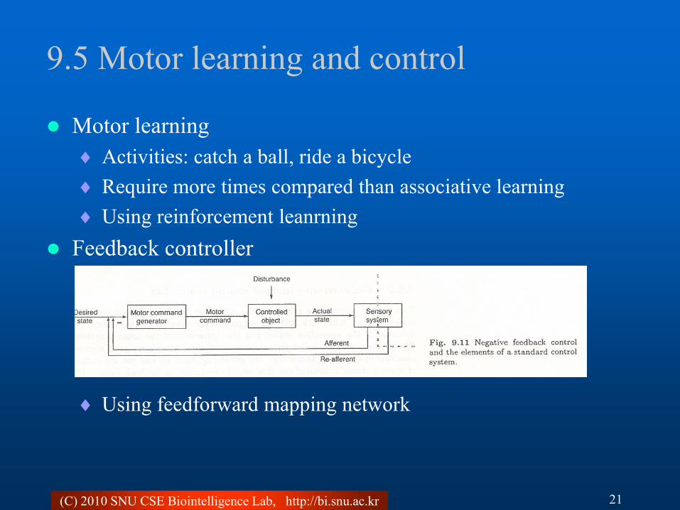
9.5 Motor learning and control
Motor learning
Activities: catch a ball, ride a bicycle
Require more times compared than associative learning
Using reinforcement leanrning
Feedback controller
Using feedforward mapping network
21

(C) 2010 SNU CSE Biointelligence Lab, http://bi.snu.ac.kr
9.5 Motor learning and control
Forward and inverse model controller
22

(C) 2010 SNU CSE Biointelligence Lab, http://bi.snu.ac.kr
9.5 Motor learning and control
The cerebellum and motor controller
23

(C) 2010 SNU CSE Biointelligence Lab, http://bi.snu.ac.kr
9.6 Reinforcement learning
Supervised learning vs. reinforcement learning
Answers vs. feedback (rewards)
Classical conditioning and the reinforcement learning problem
Conditioning
Temporal assignment problem
24

(C) 2010 SNU CSE Biointelligence Lab, http://bi.snu.ac.kr
9.6 Reinforcement learning
Formulation
Policies and value functions
r(s, a): (s: state, a: action, r: reward function)
Goal: maximizing future reward R
R(t) = summation of r(s, a) in some time window before t
Policies: π(s, a)
State value function: Vπ(s)
Action value function: Qπ(s, a)
Temporal difference learning
Off-policy vs. on-policy
25

(C) 2010 SNU CSE Biointelligence Lab, http://bi.snu.ac.kr
9.6 Reinforcement learning
Temporal delta rule
Learn from reward within neural architectures
Episodes → Vπ(s)
riin
(s): a specific pattern of rates in the input channels
wi(t): the weight in time t
26

(C) 2010 SNU CSE Biointelligence Lab, http://bi.snu.ac.kr
9.6 Reinforcement learning
Temporal difference learning
Limitation of temporal delta learning: next time step only
Different time steps
Introduction of discount factor γ (0 < γ < 1)
The perfect prediction V*
Minimizing the temporal difference error
27

(C) 2010 SNU CSE Biointelligence Lab, http://bi.snu.ac.kr
9.6 Reinforcement learning
The learning of a state value function
The learning of an action value function
28

(C) 2010 SNU CSE Biointelligence Lab, http://bi.snu.ac.kr
9.6 Reinforcement learning
Simulation MATLAB code (produce Fig. 9.16)
29

(C) 2010 SNU CSE Biointelligence Lab, http://bi.snu.ac.kr
9.6 Reinforcement learning
The actor-critic scheme and the basal ganglia
The actor-critic scheme
Temporal difference learning into a control method
Sutton and Barto proposed
Actor: the motor command generator
The adaptive critic: estimate value functions and guide
actions
30

(C) 2010 SNU CSE Biointelligence Lab, http://bi.snu.ac.kr
9.6 Reinforcement learning
The basal ganglia
Anatomical overview
31
Information stream

(C) 2010 SNU CSE Biointelligence Lab, http://bi.snu.ac.kr
9.6 Reinforcement learning
Signals of neural activities in the basal ganglia
MATLAB code for Fig. 9.20
32

(C) 2010 SNU CSE Biointelligence Lab, http://bi.snu.ac.kr
9.6 Reinforcement learning
Q-learning for the basal ganglia functions
33