9 Joint distributions and independence

9

Joint distributions and independence

Random variables related to the same experiment often influence one another.In order to capture this, we introduce the joint distribution of two or morerandom variables. We also discuss the notion of independence for randomvariables, which models the situation where random variables do not influenceeach other. As with single random variables we treat these topics for discreteand continuous random variables separately.

9.1 Joint distributions of discrete random variables

In a census one is usually interested in several variables, such as income, age,and gender. In itself these variables are interesting, but when two (or more) arestudied simultaneously, detailed information is obtained on the society wherethe census is performed. For instance, studying income, age, and gender jointlymight give insight to the emancipation of women.Without mentioning it explicitly, we already encountered several examples ofjoint distributions of discrete random variables. For example, in Chapter 4 wedefined two random variables S and M , the sum and the maximum of twoindependent throws of a die.

Quick exercise 9.1 List the elements of the event S = 7, M = 4 andcompute its probability.

In general, the joint distribution of two discrete random variables X and Y ,defined on the same sample space Ω, is given by prescribing the probabilitiesof all possible values of the pair (X, Y ).

116 9 Joint distributions and independence

Definition. The joint probability mass function p of two discreterandom variables X and Y is the function p : R

2 → [0, 1], defined by

p(a, b) = P(X = a, Y = b) for −∞ < a, b < ∞.

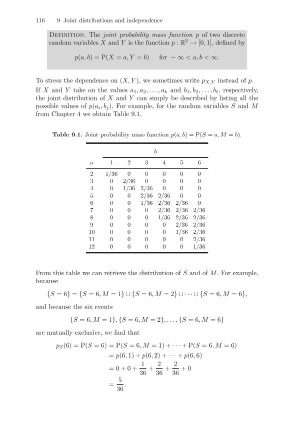
To stress the dependence on (X, Y ), we sometimes write pX,Y instead of p.If X and Y take on the values a1, a2, . . . , ak and b1, b2, . . . , b, respectively,the joint distribution of X and Y can simply be described by listing all thepossible values of p(ai, bj). For example, for the random variables S and Mfrom Chapter 4 we obtain Table 9.1.

Table 9.1. Joint probability mass function p(a, b) = P(S = a,M = b).

b

a 1 2 3 4 5 6

2 1/36 0 0 0 0 03 0 2/36 0 0 0 04 0 1/36 2/36 0 0 05 0 0 2/36 2/36 0 06 0 0 1/36 2/36 2/36 07 0 0 0 2/36 2/36 2/368 0 0 0 1/36 2/36 2/369 0 0 0 0 2/36 2/3610 0 0 0 0 1/36 2/3611 0 0 0 0 0 2/3612 0 0 0 0 0 1/36

From this table we can retrieve the distribution of S and of M . For example,because

S = 6 = S = 6, M = 1 ∪ S = 6, M = 2 ∪ · · · ∪ S = 6, M = 6,and because the six events

S = 6, M = 1, S = 6, M = 2, . . . , S = 6, M = 6are mutually exclusive, we find that

pS(6) = P(S = 6) = P(S = 6, M = 1) + · · · + P(S = 6, M = 6)= p(6, 1) + p(6, 2) + · · · + p(6, 6)

= 0 + 0 +136

+236

+236

+ 0

=536

.

9.1 Joint distributions of discrete random variables 117

Table 9.2. Joint distribution and marginal distributions of S and M .

b

a 1 2 3 4 5 6 pS(a)

2 1/36 0 0 0 0 0 1/363 0 2/36 0 0 0 0 2/364 0 1/36 2/36 0 0 0 3/365 0 0 2/36 2/36 0 0 4/366 0 0 1/36 2/36 2/36 0 5/367 0 0 0 2/36 2/36 2/36 6/368 0 0 0 1/36 2/36 2/36 5/369 0 0 0 0 2/36 2/36 4/3610 0 0 0 0 1/36 2/36 3/3611 0 0 0 0 0 2/36 2/3612 0 0 0 0 0 1/36 1/36

pM (b) 1/36 3/36 5/36 7/36 9/36 11/36 1

Thus we see that the probabilities of S can be obtained by taking the sumof the joint probabilities in the rows of Table 9.1. This yields the probabilitydistribution of S, i.e., all values of pS(a) for a = 2, . . . , 12. We speak of themarginal distribution of S. In Table 9.2 we have added this distribution in theright “margin” of the table. Similarly, summing over the columns of Table 9.1yields the marginal distribution of M , in the bottom margin of Table 9.2.The joint distribution of two random variables contains a lot more informationthan the two marginal distributions. This can be illustrated by the fact that inmany cases the joint probability mass function of X and Y cannot be retrievedfrom the marginal probability mass functions pX and pY . A simple exampleis given in the following quick exercise.

Quick exercise 9.2 Let X and Y be two discrete random variables, withjoint probability mass function p, given by the following table, where ε is anarbitrary number between −1/4 and 1/4.

b

a 0 1 pX(a)

0 1/4 − ε 1/4 + ε . . .1 1/4 + ε 1/4 − ε . . .

pY (b) . . . . . . . . .

Complete the table, and conclude that we cannot retrieve p from pX and pY .


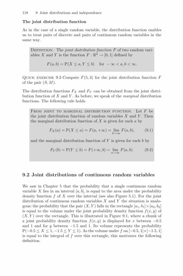
The joint distribution function

As in the case of a single random variable, the distribution function enablesus to treat pairs of discrete and pairs of continuous random variables in thesame way.

Definition. The joint distribution function F of two random vari-ables X and Y is the function F : R

2 → [0, 1] defined by

F (a, b) = P(X ≤ a, Y ≤ b) for −∞ < a, b < ∞.

Quick exercise 9.3 Compute F (5, 3) for the joint distribution function Fof the pair (S, M).

The distribution functions FX and FY can be obtained from the joint distri-bution function of X and Y . As before, we speak of the marginal distributionfunctions. The following rule holds.

From joint to marginal distribution function. Let F bethe joint distribution function of random variables X and Y . Thenthe marginal distribution function of X is given for each a by

FX(a) = P(X ≤ a) = F (a, +∞) = limb→∞

F (a, b), (9.1)

and the marginal distribution function of Y is given for each b by

FY (b) = P(Y ≤ b) = F (+∞, b) = lima→∞ F (a, b). (9.2)

9.2 Joint distributions of continuous random variables

We saw in Chapter 5 that the probability that a single continuous randomvariable X lies in an interval [a, b], is equal to the area under the probabilitydensity function f of X over the interval (see also Figure 5.1). For the jointdistribution of continuous random variables X and Y the situation is analo-gous: the probability that the pair (X, Y ) falls in the rectangle [a1, b1]×[a2, b2]is equal to the volume under the joint probability density function f(x, y) of(X, Y ) over the rectangle. This is illustrated in Figure 9.1, where a chunk ofa joint probability density function f(x, y) is displayed for x between −0.5and 1 and for y between −1.5 and 1. Its volume represents the probabilityP(−0.5 ≤ X ≤ 1,−1.5 ≤ Y ≤ 1). As the volume under f on [−0.5, 1]×[−1.5, 1]is equal to the integral of f over this rectangle, this motivates the followingdefinition.

9.2 Joint distributions of continuous random variables 119

-3-2

-1 0

12

3

x-3

-2-1

01

23

y

00.0

50.1

0.1

5

f(x,y)

Fig. 9.1. Volume under a joint probability density function f on the rectangle[−0.5, 1] × [−1.5, 1].

Definition. Random variables X and Y have a joint continuousdistribution if for some function f : R

2 → R and for all numbersa1, a2 and b1, b2 with a1 ≤ b1 and a2 ≤ b2,

P(a1 ≤ X ≤ b1, a2 ≤ Y ≤ b2) =∫ b1

a1

∫ b2

a2

f(x, y) dxdy.

The function f has to satisfy f(x, y) ≥ 0 for all x and y, and∫∞−∞

∫∞−∞ f(x, y) dxdy = 1. We call f the joint probability density

function of X and Y .

As in the one-dimensional case there is a simple relation between the jointdistribution function F and the joint probability density function f :

F (a, b) =∫ a

−∞

∫ b

−∞f(x, y) dxdy and f(x, y) =

∂2

∂x∂yF (x, y).

A joint probability density function of two random variables is also calleda bivariate probability density. An explicit example of such a density is thefunction

f(x, y) =30π

e−50x2−50y2+80xy

for −∞ < x < ∞ and −∞ < y < ∞; see Figure 9.2. This is an example ofa bivariate normal density (see Remark 11.2 for a full description of bivariatenormal distributions).We illustrate a number of properties of joint continuous distributions by meansof the following simple example. Suppose that X and Y have joint probability


-0.4

-0.2

0

0.20.4

X-0.4

-0.2

0

0.2

0.4

Y

02

46

810

f(x,y

)

Fig. 9.2. A bivariate normal probability density function.

density function

f(x, y) =275(2x2y + xy2

)for 0 ≤ x ≤ 3 and 1 ≤ y ≤ 2,

and f(x, y) = 0 otherwise; see Figure 9.3.

4

3

203

0,2

2,5 x1

0,4

2

0,6

1,5y

0

0,8

1

1

0,5 -1

1,2

0

Fig. 9.3. The probability density function f(x, y) = 275

(2x2y + xy2

).

9.2 Joint distributions of continuous random variables 121

As an illustration of how to compute joint probabilities:

P(

1 ≤ X ≤ 2,43≤ Y ≤ 5

3

)=∫ 2

1

∫ 53

43

f(x, y) dxdy

=275

∫ 2

1

(∫ 53

43

(2x2y + xy2) dy

)dx

=275

∫ 2

1

(x2 +

6181

x

)dx =

1872025

.

Next, for a between 0 and 3 and b between 1 and 2, we determine the ex-pression of the joint distribution function. Since f(x, y) = 0 for x < 0 ory < 1,

F (a, b) = P(X ≤ a, Y ≤ b) =∫ a

−∞

(∫ b

−∞f(x, y) dy

)dx

=275

∫ a

0

(∫ b

1

(2x2y + xy2) dy

)dx

=1

225(2a3b2 − 2a3 + a2b3 − a2

).

Note that for either a outside [0, 3] or b outside [1, 2], the expression for F (a, b)is different. For example, suppose that a is between 0 and 3 and b is largerthan 2. Since f(x, y) = 0 for y > 2, we find for any b ≥ 2:

F (a, b) = P(X ≤ a, Y ≤ b) = P(X ≤ a, Y ≤ 2) = F (a, 2) =1

225(6a3 + 7a2

).

Hence, applying (9.1) one finds the marginal distribution function of X :

FX(a) = limb→∞

F (a, b) =1

225(6a3 + 7a2

)for a between 0 and 3.

Quick exercise 9.4 Show that FY (b) = 175

(3b3 + 18b2 − 21

)for b between 1

and 2.

The probability density of X can be found by differentiating FX :

fX(x) =ddx

FX(x) =ddx

(1

225(6x3 + 7x2

))=

2225

(9x2 + 7x

)for x between 0 and 3. It is also possible to obtain the probability densityfunction of X directly from f(x, y). Recall that we determined marginal prob-abilities of discrete random variables by summing over the joint probabilities(see Table 9.2). In a similar way we can find fX . For x between 0 and 3,


fX(x) =∫ ∞

−∞f(x, y) dy =

275

∫ 2

1

(2x2y + xy2

)dy =

2225

(9x2 + 7x

).

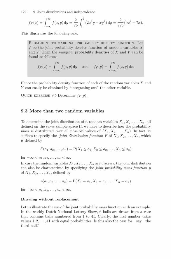
This illustrates the following rule.

From joint to marginal probability density function. Letf be the joint probability density function of random variables Xand Y . Then the marginal probability densities of X and Y can befound as follows:

fX(x) =∫ ∞

−∞f(x, y) dy and fY (y) =

∫ ∞

−∞f(x, y) dx.

Hence the probability density function of each of the random variables X andY can easily be obtained by “integrating out” the other variable.

Quick exercise 9.5 Determine fY (y).

9.3 More than two random variables

To determine the joint distribution of n random variables X1, X2, . . . , Xn, alldefined on the same sample space Ω, we have to describe how the probabilitymass is distributed over all possible values of (X1, X2, . . . , Xn). In fact, itsuffices to specify the joint distribution function F of X1, X2, . . . , Xn, whichis defined by

F (a1, a2, . . . , an) = P(X1 ≤ a1, X2 ≤ a2, . . . , Xn ≤ an)

for −∞ < a1, a2, . . . , an < ∞.In case the random variables X1, X2, . . . , Xn are discrete, the joint distributioncan also be characterized by specifying the joint probability mass function pof X1, X2, . . . , Xn, defined by

p(a1, a2, . . . , an) = P(X1 = a1, X2 = a2, . . . , Xn = an)

for −∞ < a1, a2, . . . , an < ∞.

Drawing without replacement

Let us illustrate the use of the joint probability mass function with an example.In the weekly Dutch National Lottery Show, 6 balls are drawn from a vasethat contains balls numbered from 1 to 41. Clearly, the first number takesvalues 1, 2, . . . , 41 with equal probabilities. Is this also the case for—say—thethird ball?

9.3 More than two random variables 123

Let us consider a more general situation. Suppose a vase contains balls num-bered 1, 2, . . . , N . We draw n balls without replacement from the vase. Notethat n cannot be larger than N . Each ball is selected with equal probability,i.e., in the first draw each ball has probability 1/N , in the second draw each ofthe N −1 remaining balls has probability 1/(N −1), and so on. Let Xi denotethe number on the ball in the i-th draw, for i = 1, 2, . . . , n. In order to obtainthe marginal probability mass function of Xi, we first compute the joint proba-bility mass function of X1, X2, . . . , Xn. Since there are N(N−1) · · · (N−n+1)possible combinations for the values of X1, X2, . . . , Xn, each having the sameprobability, the joint probability mass function is given by

p(a1, a2, . . . , an) = P(X1 = a1, X2 = a2, . . . , Xn = an)

=1

N(N − 1) · · · (N − n + 1),

for all distinct values a1, a2, . . . , an with 1 ≤ aj ≤ N . Clearly X1, X2, . . . , Xn

influence each other. Nevertheless, the marginal distribution of each Xi isthe same. This can be seen as follows. Similar to obtaining the marginalprobability mass functions in Table 9.2, we can find the marginal probabilitymass function of Xi by summing the joint probability mass function over allpossible values of X1, . . . , Xi−1, Xi+1, . . . , Xn:

pXi(k) =∑

p(a1, . . . , ai−1, k, ai+1, . . . , an)

=∑ 1

N(N − 1) · · · (N − n + 1),

where the sum runs over all distinct values a1, a2, . . . , an with 1 ≤ aj ≤ Nand ai = k. Since there are (N − 1)(N − 2) · · · (N −n+1) such combinations,we conclude that the marginal probability mass function of Xi is given by

pXi(k) = (N − 1)(N − 2) · · · (N − n + 1) · 1N(N − 1) · · · (N − n + 1)

=1N

,

for k = 1, 2, . . . , N . We see that the marginal probability mass function ofeach Xi is the same, assigning equal probability 1/N to each possible value.In case the random variables X1, X2, . . . , Xn are continuous, the joint dis-tribution is defined in a similar way as in the case of two variables. We saythat the random variables X1, X2, . . . , Xn have a joint continuous distribu-tion if for some function f : R

n → R and for all numbers a1, a2, . . . , an andb1, b2, . . . , bn with ai ≤ bi,

P(a1 ≤ X1 ≤ b1, a2 ≤ X2 ≤ b2, . . . , an ≤ Xn ≤ bn)

=∫ b1

a1

∫ b2

a2

· · ·∫ bn

an

f(x1, x2, . . . , xn) dx1 dx2 · · · dxn.

Again f has to satisfy f(x1, x2, . . . , xn) ≥ 0 and f has to integrate to 1. Wecall f the joint probability density of X1, X2, . . . , Xn.


9.4 Independent random variables

In earlier chapters we have spoken of independence of random variables, an-ticipating a formal definition. On page 46 we postulated that the events

R1 = a1, R2 = a2, . . . , R10 = a10

related to the Bernoulli random variables R1, . . . , R10 are independent. Howshould one define independence of random variables? Intuitively, random vari-ables X and Y are independent if every event involving only X is indepen-dent of every event involving only Y . Since for two discrete random variablesX and Y , any event involving X and Y is the union of events of the typeX = a, Y = b, an adequate definition for independence would be

P(X = a, Y = b) = P(X = a) P(Y = b) , (9.3)

for all possible values a and b. However, this definition is useless for continuousrandom variables. Both the discrete and the continuous case are covered bythe following definition.

Definition. The random variables X and Y , with joint distributionfunction F , are independent if

P(X ≤ a, Y ≤ b) = P(X ≤ a) P(Y ≤ b) ,

that is,F (a, b) = FX(a)FY (b) (9.4)

for all possible values a and b. Random variables that are not inde-pendent are called dependent.

Note that independence of X and Y guarantees that the joint probability ofX ≤ a, Y ≤ b factorizes. More generally, the following is true: if X and Yare independent, then

P(X ∈ A, Y ∈ B) = P(X ∈ A) P(Y ∈ B) , (9.5)

for all suitable A and B, such as intervals and points. As a special case wecan take A = a, B = b, which yields that for independent X and Y theprobability of X = a, Y = b equals the product of the marginal probabilities.In fact, for discrete random variables the definition of independence can bereduced—after cumbersome computations—to equality (9.3). For continuousrandom variables X and Y we find, differentiating both sides of (9.4) withrespect to x and y, that

f(x, y) = fX(x)fY (y).

9.5 Propagation of independence 125

Quick exercise 9.6 Determine for which value of ε the discrete randomvariables X and Y from Quick exercise 9.2 are independent.

More generally, random variables X1, X2, . . . , Xn, with joint distribution func-tion F , are independent if for all values a1, . . . , an,

F (a1, a2, . . . , an) = FX1 (a1)FX2 (a2) · · ·FXn(an).

As in the case of two discrete random variables, the discrete random variablesX1, X2, . . . , Xn are independent if

P(X1 = a1, . . . , Xn = an) = P(X1 = a1) · · ·P(Xn = an) ,

for all possible values a1, . . . , an. Thus we see that the definition of inde-pendence for discrete random variables is in agreement with our intuitiveinterpretation given earlier in (9.3).In case of independent continuous random variables X1, X2, . . . , Xn with jointprobability density function f , differentiating the joint distribution functionwith respect to all the variables gives that

f(x1, x2, . . . , xn) = fX1(x1)fX2(x2) · · · fXn(xn) (9.6)

for all values x1, . . . , xn. By integrating both sides over (−∞, a1]× (−∞, a2]×· · ·×(−∞, an], we find the definition of independence. Hence in the continuouscase, (9.6) is equivalent to the definition of independence.

9.5 Propagation of independence

A natural question is whether transformed independent random variables areagain independent. We start with a simple example. Let X and Y be twoindependent random variables with joint distribution function F . Take aninterval I = (a, b] and define random variables U and V as follows:

U =

1 if X ∈ I

0 if X /∈ I,and V =

1 if Y ∈ I

0 if Y /∈ I.

Are U and V independent? Yes, they are! By using (9.5) and the independenceof X and Y , we can write

P(U = 0, V = 1) = P(X ∈ Ic, Y ∈ I)= P(X ∈ Ic) P(Y ∈ I)= P(U = 0)P(V = 1) .

By a similar reasoning one finds that for all values a and b,


P(U = a, V = b) = P(U = a) P(V = b) .

This illustrates the fact that for independent random variables X1, X2, . . . , Xn,the random variables Y1, Y2, . . . , Yn, where each Yi is determined by Xi only,inherit the independence from the Xi. The general rule is given here.

Propagation of independence. Let X1, X2, . . . , Xn be indepen-dent random variables. For each i, let hi : R → R be a function anddefine the random variable

Yi = hi(Xi).

Then Y1, Y2, . . . , Yn are also independent.

Often one uses this rule with all functions the same: hi = h. For instance, inthe preceding example,

h(x) =

1 if x ∈ I

0 if x /∈ I.

The rule is also useful when we need different transformations for differentXi. We already saw an example of this in Chapter 6. In the single-serverqueue example in Section 6.4, the Exp(0.5) random variables T1, T2, . . . andU(2, 5) random variables S1, S2, . . . are required to be independent. They aregenerated according to the technique described in Section 6.2. With a se-quence U1, U2, . . . of independent U(0, 1) random variables we can accomplishindependence of the Ti and Si as follows:

Ti = F inv(U2i−1) and Si = Ginv(U2i),

where F and G are the distribution functions of the Exp(0.5) distribution andthe U(2, 5) distribution. The propagation-of-independence rule now guaran-tees that all random variables T1, S1, T2, S2, . . . are independent.

9.6 Solutions to the quick exercises

9.1 The only possibilities with the sum equal to 7 and the maximum equalto 4 are the combinations (3, 4) and (4, 3). They both have probability 1/36,so that P(S = 7, M = 4) = 2/36.

9.2 Since pX(0), pX(1), pY (0), and pY (1) are all equal to 1/2, knowing onlypX and pY yields no information on ε whatsoever. You have to be a studentat Hogwarts to be able to get the values of p right!

9.3 Since S and M are discrete random variables, F (5, 3) is the sum of theprobabilities P(S = a, M = b) of all combinations (a, b) with a ≤ 5 and b ≤ 3.From Table 9.2 we see that this sum is 8/36.

9.7 Exercises 127

9.4 For a between 0 and 3 and for b between 1 and 2, we have seen that

F (a, b) =1

225(2a3b2 − 2a3 + a2b3 − a2

).

Since f(x, y) = 0 for x > 3, we find for any a ≥ 3 and b between 1 and 2:

F (a, b) = P(X ≤ a, Y ≤ b) = P(X ≤ 3, Y ≤ b)

= F (3, b) =175(3b3 + 18b2 − 21

).

As a result, applying (9.2) yields that FY (b) = lima→∞ F (a, b) = F (3, b) =175

(3b3 + 18b2 − 21

), for b between 1 and 2.

9.5 For y between 1 and 2, we have seen that FY (y) = 175

(3y3 + 18y2 − 21

).

Differentiating with respect to y yields that

fY (y) =ddy

FY (y) =125

(3y2 + 12y),

for y between 1 and 2 (and fY (y) = 0 otherwise). The probability densityfunction of Y can also be obtained directly from f(x, y). For y between 1and 2:

fY (y) =∫ ∞

−∞f(x, y) dx =

275

∫ 3

0

(2x2y + xy2) dx

=275[23x3y +

12x2y2

]x=3

x=0=

125

(3y2 + 12y).

Since f(x, y) = 0 for values of y not between 1 and 2, we have that fY (y) =∫∞−∞ f(x, y) dx = 0 for these y’s.

9.6 The number ε is between −1/4 and 1/4. Now X and Y are independentin case p(i, j) = P(X = i, Y = j) = P(X = i)P(Y = j) = pX(i)pY (j), for alli, j = 0, 1. If i = j = 0, we should have

14− ε = p(0, 0) = pX(0) pY (0) =

14.

This implies that ε = 0. Furthermore, for all other combinations (i, j) onecan check that for ε = 0 also p(i, j) = pX(i) pY (j), so that X and Y areindependent. If ε = 0, we have p(0, 0) = pX(0) pY (0), so that X and Y aredependent.

9.7 Exercises

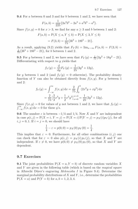
9.1 The joint probabilities P(X = a, Y = b) of discrete random variables Xand Y are given in the following table (which is based on the magical squarein Albrecht Durer’s engraving Melencolia I in Figure 9.4). Determine themarginal probability distributions of X and Y , i.e., determine the probabilitiesP(X = a) and P(Y = b) for a, b = 1, 2, 3, 4.


Fig. 9.4. Albrecht Durer’s Melencolia I.

Albrecht Durer (German, 1471-1528) Melencolia I, 1514. Engraving. Bequestof William P. Chapman, Jr., Class of 1895. Courtesy of the Herbert F. JohnsonMuseum of Art, Cornell University.

a

b 1 2 3 4

1 16/136 3/136 2/136 13/1362 5/136 10/136 11/136 8/1363 9/136 6/136 7/136 12/1364 4/136 15/136 14/136 1/136

9.7 Exercises 129

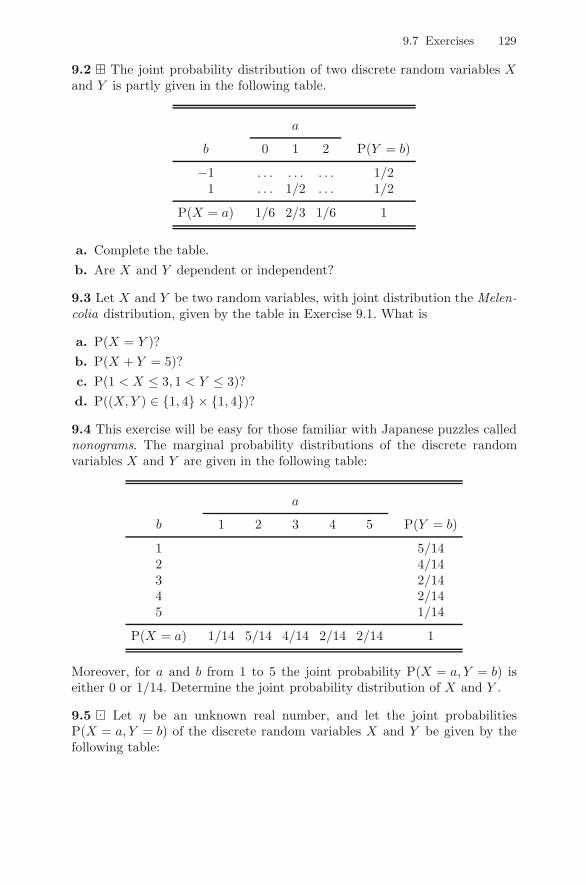
9.2 The joint probability distribution of two discrete random variables Xand Y is partly given in the following table.

a

b 0 1 2 P(Y = b)

−1 . . . . . . . . . 1/21 . . . 1/2 . . . 1/2

P(X = a) 1/6 2/3 1/6 1

a. Complete the table.b. Are X and Y dependent or independent?

9.3 Let X and Y be two random variables, with joint distribution the Melen-colia distribution, given by the table in Exercise 9.1. What is

a. P(X = Y )?b. P(X + Y = 5)?c. P(1 < X ≤ 3, 1 < Y ≤ 3)?d. P((X, Y ) ∈ 1, 4 × 1, 4)?9.4 This exercise will be easy for those familiar with Japanese puzzles callednonograms. The marginal probability distributions of the discrete randomvariables X and Y are given in the following table:

a

b 1 2 3 4 5 P(Y = b)

1 5/142 4/143 2/144 2/145 1/14

P(X = a) 1/14 5/14 4/14 2/14 2/14 1

Moreover, for a and b from 1 to 5 the joint probability P(X = a, Y = b) iseither 0 or 1/14. Determine the joint probability distribution of X and Y .

9.5 Let η be an unknown real number, and let the joint probabilitiesP(X = a, Y = b) of the discrete random variables X and Y be given by thefollowing table:


a

b −1 0 1

4 η − 116

14 − η 0

5 18

316

18

6 η + 116

116

14 − η

a. Which are the values η can attain?b. Is there a value of η for which X and Y are independent?

9.6 Let X and Y be two independent Ber(12 ) random variables. Define

random variables U and V by:

U = X + Y and V = |X − Y |.a. Determine the joint and marginal probability distributions of U and V .b. Find out whether U and V are dependent or independent.

9.7 To investigate the relation between hair color and eye color, the hair colorand eye color of 5383 persons was recorded. The data are given in the followingtable:

Hair color

Eye color Fair/red Medium Dark/black

Light 1168 825 305Dark 573 1312 1200

Source: B. Everitt and G. Dunn. Applied multivariate data analysis. Secondedition Hodder Arnold, 2001; Table 4.12. Reproduced by permission of Hodder& Stoughton.

Eye color is encoded by the values 1 (Light) and 2 (Dark), and hair color by1 (Fair/red), 2 (Medium), and 3 (Dark/black). By dividing the numbers inthe table by 5383, the table is turned into a joint probability distribution forrandom variables X (hair color) taking values 1 to 3 and Y (eye color) takingvalues 1 and 2.

a. Determine the joint and marginal probability distributions of X and Y .b. Find out whether X and Y are dependent or independent.

9.8 Let X and Y be independent random variables with probability distri-butions given by

P(X = 0) = P(X = 1) = 12 and P(Y = 0) = P(Y = 2) = 1

2 .

9.7 Exercises 131

a. Compute the distribution of Z = X + Y .b. Let Y and Z be independent random variables, where Y has the same

distribution as Y , and Z the same distribution as Z. Compute the distri-bution of X = Z − Y .

9.9 Suppose that the joint distribution function of X and Y is given by

F (x, y) = 1 − e−2x − e−y + e−(2x+y) if x > 0, y > 0,

and F (x, y) = 0 otherwise.

a. Determine the marginal distribution functions of X and Y .b. Determine the joint probability density function of X and Y .c. Determine the marginal probability density functions of X and Y .d. Find out whether X and Y are independent.

9.10 Let X and Y be two continuous random variables with joint proba-bility density function

f(x, y) =125

xy(1 + y) for 0 ≤ x ≤ 1 and 0 ≤ y ≤ 1,

and f(x, y) = 0 otherwise.

a. Find the probability P(

14 ≤ X ≤ 1

2 , 13 ≤ Y ≤ 2

3

).

b. Determine the joint distribution function of X and Y for a and b between0 and 1.

c. Use your answer from b to find FX(a) for a between 0 and 1.d. Apply the rule on page 122 to find the probability density function of X

from the joint probability density function f(x, y). Use the result to verifyyour answer from c.

e. Find out whether X and Y are independent.

9.11 Let X and Y be two continuous random variables, with the samejoint probability density function as in Exercise 9.10. Find the probabilityP(X < Y ) that X is smaller than Y .

9.12 The joint probability density function f of the pair (X, Y ) is given by

f(x, y) = K(3x2 + 8xy) for 0 ≤ x ≤ 1 and 0 ≤ y ≤ 2,

and f(x, y) = 0 for all other values of x and y. Here K is some positiveconstant.

a. Find K.b. Determine the probability P(2X ≤ Y ).


9.13 On a disc with origin (0, 0) and radius 1, a point (X, Y ) is selected bythrowing a dart that hits the disc in an arbitrary place. This is best describedby the joint probability density function f of X and Y , given by

f(x, y) =

c if x2 + y2 ≤ 10 otherwise,

where c is some positive constant.

a. Determine c.b. Let R =

√X2 + Y 2 be the distance from (X, Y ) to the origin. Determine

the distribution function FR.c. Determine the marginal density function fX . Without doing any calcula-

tions, what can you say about fY ?

9.14 An arbitrary point (X, Y ) is drawn from the square [−1, 1] × [−1, 1].This means that for any region G in the plane, the probability that (X, Y ) isin G, is given by the area of G∩ divided by the area of , where denotesthe square [−1, 1]× [−1, 1]:

P((X, Y ) ∈ G) =area of G ∩

area of .

a. Determine the joint probability density function of the pair (X, Y ).b. Check that X and Y are two independent, U(−1, 1) distributed random

variables.

9.15 Let the pair (X, Y ) be drawn arbitrarily from the triangle ∆ withvertices (0, 0), (0, 1), and (1, 1).

a. Use Figure 9.5 to show that the joint distribution function F of the pair(X, Y ) satisfies

F (a, b) =

⎧⎪⎪⎪⎪⎪⎪⎨⎪⎪⎪⎪⎪⎪⎩

0 for a or b less than 0a(2b − a) for (a, b) in the triangle ∆b2 for b between 0 and 1 and a larger than b

2a − a2 for a between 0 and 1 and b larger than 11 for a and b larger than 1.

b. Determine the joint probability density function f of the pair (X, Y ).c. Show that fX(x) = 2− 2x for x between 0 and 1 and that fY (y) = 2y for

y between 0 and 1.

9.16 (Continuation of Exercise 9.15) An arbitrary point (U, V ) is drawn fromthe unit square [0, 1]× [0, 1]. Let X and Y be defined as in Exercise 9.15. Showthat minU, V has the same distribution as X and that maxU, V has thesame distribution as Y .

9.7 Exercises 133

(0, 0)

(0, 1) (1, 1)

(a, b)•∆

←− Rectangle (−∞, a] × (−∞, b]...................

.

.

.

.

.

.

.

.

.

.

.

.

.

.

.

.

.

.

.

.

.

.

.

.

.

.

.

.

.

.

.

.

.

.

.

.

.

.

.

.

.

.

.

.

.

.

.

.

.

.

.

.

.

.

.

.

.

.

.

.

.

.

.

.

.

.

.

.

.

.

.

.

.

.

.

.

.

.

.

.

.

.

.

.

.

.

.

.

.

.

.

.

.

.

.

.

.

.

.

.

.

.

.

.

.

.

.

.

.

.

.

.

.

.

.

.

.

.

.

.

.

.

.

.

.

.

.

.

.

.

.

.

.

.

.

.

.

.

.

.

.

.

.

.

.

.

.

.

.

.

.

.

.

.

.

.

.

.

.

.

.

.

.

.

.

.

.

.

.

.

.

.

.

.

.

.

.

.

.

.

.

.

.

.

.

.

.

.

.

.

.

.

.

.

.

.

.

.

.

.

.

.

.

.

.

.....................................................................................................................................................................................................................................................................................................................................................................

Fig. 9.5. Drawing (X, Y ) from (−∞, a] × (−∞, b] ∩ ∆.

9.17 Let U1 and U2 be two independent random variables, both uniformlydistributed over [0, a]. Let V = minU1, U2 and Z = maxU1, U2. Showthat the joint distribution function of V and Z is given by

F (s, t) = P(V ≤ s, Z ≤ t) =t2 − (t − s)2

a2for 0 ≤ s ≤ t ≤ a.

Hint : note that V ≤ s and Z ≤ t happens exactly when both U1 ≤ t andU2 ≤ t, but not both s < U1 ≤ t and s < U2 ≤ t.

9.18 Suppose a vase contains balls numbered 1, 2, . . . , N . We draw n ballswithout replacement from the vase. Each ball is selected with equal probability,i.e., in the first draw each ball has probability 1/N , in the second draw eachof the N − 1 remaining balls has probability 1/(N − 1), and so on. For i =1, 2, . . . , n, let Xi denote the number on the ball in the ith draw. We haveshown that the marginal probability mass function of Xi is given by

pXi(k) =1N

, for k = 1, 2, . . . , N.

a. Show thatE[Xi] =

N + 12

.

b. Compute the variance of Xi. You may use the identity

1 + 4 + 9 + · · · + N2 =16N(N + 1)(2N + 1).

9.19 Let X and Y be two continuous random variables, with joint proba-bility density function

f(x, y) =30π

e−50x2−50y2+80xy

for −∞ < x < ∞ and −∞ < y < ∞; see also Figure 9.2.


a. Determine positive numbers a, b, and c such that

50x2 − 80xy + 50y2 = (ay − bx)2 + cx2.

b. Setting µ = 45x, and σ = 1

10 , show that

(√

50y −√

32x)2 =12

(y − µ

σ

)2

and use this to show that∫ ∞

−∞e−(

√50y−√

32x)2 dy =√

2π

10.

c. Use the results from b to determine the probability density function fX

of X . What kind of distribution does X have?

9.20 Suppose we throw a needle on a large sheet of paper, on which horizontallines are drawn, which are at needle-length apart (see also Exercise 21.16).Choose one of the horizontal lines as x-axis, and let (X, Y ) be the center of theneedle. Furthermore, let Z be the distance of this center (X, Y ) to the nearesthorizontal line under (X, Y ), and let H be the angle between the needle andthe positive x-axis.

a. Assuming that the length of the needle is equal to 1, argue that Z hasa U(0, 1) distribution. Also argue that H has a U(0, π) distribution andthat Z and H are independent.

b. Show that the needle hits a horizontal line when

Z ≤ 12

sin H or 1 − Z ≤ 12

sin H.

c. Show that the probability that the needle will hit one of the horizontallines equals 2/π.

9 Joint distributions and independence

Documents

Transcript of 9 Joint distributions and independence