8.942 Cosmology Notes

Andy Lutomirski

This copy is from 2008-11-18 15:32:35 -0500 (Tue, 18 Nov 2008).

Contents

1 Introduction 21.1 GR . . . . . . . . . . . . . . . . . . . . . . . . . . . . . . . . . . . 2

2 Zero-order cosmology 32.1 The FLRW metric . . . . . . . . . . . . . . . . . . . . . . . . . . 32.2 Derivation of the FRW metric . . . . . . . . . . . . . . . . . . . . 42.3 Conformal time . . . . . . . . . . . . . . . . . . . . . . . . . . . . 52.4 Testable implications . . . . . . . . . . . . . . . . . . . . . . . . . 52.5 Controversies . . . . . . . . . . . . . . . . . . . . . . . . . . . . . 52.6 Angular diameter distance and luminosity distance . . . . . . . . 6

3 Inflation 73.1 The horizon and flatness problems . . . . . . . . . . . . . . . . . 73.2 Inflation with a scalar field . . . . . . . . . . . . . . . . . . . . . 73.3 Interpretation of the potential V (φ) . . . . . . . . . . . . . . . . 93.4 Evidence for inflation . . . . . . . . . . . . . . . . . . . . . . . . . 93.5 Crazy effects of inflation . . . . . . . . . . . . . . . . . . . . . . . 9

3.5.1 The landscape view . . . . . . . . . . . . . . . . . . . . . 93.5.2 Eternal inflation . . . . . . . . . . . . . . . . . . . . . . . 103.5.3 Measure problem and the A-word . . . . . . . . . . . . . . 10

3.6 Reheating . . . . . . . . . . . . . . . . . . . . . . . . . . . . . . . 11

4 Big bang nucleosynthesis 114.1 Basics . . . . . . . . . . . . . . . . . . . . . . . . . . . . . . . . . 114.2 Thermal equilibrium . . . . . . . . . . . . . . . . . . . . . . . . . 124.3 Important temperatures . . . . . . . . . . . . . . . . . . . . . . . 124.4 BBN Reactions . . . . . . . . . . . . . . . . . . . . . . . . . . . . 134.5 WIMPs . . . . . . . . . . . . . . . . . . . . . . . . . . . . . . . . 13

5 The universe to 1st order 145.1 Newtonian analysis . . . . . . . . . . . . . . . . . . . . . . . . . . 145.2 Measuring the power spectrum . . . . . . . . . . . . . . . . . . . 15

1

6 The transfer function T (z, k) 166.1 Multi-component perturbation growth . . . . . . . . . . . . . . . 166.2 Neutrinos . . . . . . . . . . . . . . . . . . . . . . . . . . . . . . . 17

7 The cosmic microwave background 187.1 Observations . . . . . . . . . . . . . . . . . . . . . . . . . . . . . 187.2 The CMB fluctuation formula . . . . . . . . . . . . . . . . . . . . 187.3 Spherical harmonics . . . . . . . . . . . . . . . . . . . . . . . . . 207.4 Projection effects . . . . . . . . . . . . . . . . . . . . . . . . . . . 217.5 Nonlinear effects . . . . . . . . . . . . . . . . . . . . . . . . . . . 217.6 Seeing other effects . . . . . . . . . . . . . . . . . . . . . . . . . . 22

7.6.1 ISW . . . . . . . . . . . . . . . . . . . . . . . . . . . . . . 227.6.2 Global reionization . . . . . . . . . . . . . . . . . . . . . . 227.6.3 Local reionization . . . . . . . . . . . . . . . . . . . . . . 22

7.7 CMB polarization . . . . . . . . . . . . . . . . . . . . . . . . . . 227.8 Measuring the CMB . . . . . . . . . . . . . . . . . . . . . . . . . 23

8 Lensing 23

9 The Lyman α forest 25

10 21-cm tomography 25

1 Introduction

These are my notes from Max Tegmark’s 8.942 (Cosmology) lectures at MIT inthe fall of 2008-09. I’m typing them in class and they aren’t very well edited, sothey almost certainly contain errors and omissions. I hope that they are usefulnonetheless.

This work is licensed under the Creative Commons Attribution-Noncommercial-Share Alike 3.0 United States License. To view a copy of this license, visithttp://creativecommons.org/licenses/by-nc-sa/3.0/us/ or send a letterto Creative Commons, 171 Second Street, Suite 300, San Francisco, California,94105, USA.

If you want a copy of the LYX or LATEX source, ask me.

1.1 GR

The formula for gravitational redshift is

∆νν

=gh

c2=

φ

c2→ dτ

dt= (1 + φ) ,

so the metric for Newtonian gravity is

dτ2 = (1 + 2φ) dt2 − dx2 − dy2 − dz2.

2

Objects in free fall follow geodesics — that is, they try to maximize theirown aging. So a falling object has to balance time dilation with the gravitationalredshift. The total aging is

τ =dτ =

B

A

√(1 + 2φ)− x2 − y2 − z2dt

= tB

tA

f (t, x, x) dt

≈ tB

tA

(1 + φ− x2

2

)dt.

2 Zero-order cosmology

2.1 The FLRW metric

The FLRW metric is

dτ2 = dt2 − a (t)2

(dr2

1− kr2+ r2dθ2 + r2 sin2 θdφ2

).

= dt2 − a (t)2

[dr2

1− kr2+ dΩ2

],

where k = 0,±1 and, if k = 1, r is bounded.Hubble noticed that objects seemed to recede at velocity proportional to their

distance. (There were all kinds of problems with his paper, but he was right inhis conclusion. Einstein objected to Lemetre’s idea of an expanding universe atfirst—there was a tendency for people not to believe their own equations.)

An object is said to be comoving if its (r, θ, φ) coordinates are constant. Thedistance scales as d = d0

a(t)a0(t) , so v = d = d0

a(t)a(t0) and v

d = aa = H, the Hubble

parameter.

H =d

dtln a (1)

H used to be called the Hubble constant, but it isn’t constant. The other majorparameter is the redshift z = a0

a − 1.If you plug the FLRW metric into the EFE, you end up with the Friedman

equation

H2 =(a

a

)2

=8πG

3ρ− kc2

a2=

8πG3

ρtot.

The solution depends on what kind of stuff there is. We’ll consider matter,radiation, curvature, and the vacuum.

Matter ρ ∝ 1a3 to conserve mass. This works for normal matter and for dark

matter.

Radiation ρ ∝ 1a4 because the number density falls off like a−3 but the redshift

adds another factor of a−1. This applies to any ultrarelativistic particles.

3

Vacuum ρ is constant. It turns out that this stuff has negative pressure, soenergy is still conserved.

Curvature ρ ∝ a−2 by reading the equation. The sign of this term can vary.

We can solve the Friedman equation easily if we ignore all but one term. In thematter-dominated case, we get a ∝ t2/3. For radiation, a ∝ t1/2. For curvature,with k = −1, a ∝ t, which turns out to be equivalent to Minkowski space. Forvacuum-dominated space, a ∝ eHt.

H (z) is the most convenient parameterization, because z is easy to measure.We can write

H2 =8πG

3(ργ + ρm + ρk + ρΛ) = H2

0

[Ωγ (1 + z)4 + Ωm (1 + z)3 + Ωk (1 + z)2 + ΩΛ

],

where ρ∗ ≡ 3H20

8πG and Ωi ≡ ρiρ∗

We can write Ωtot = 1− Ωk.To compute the ages of things, we write

dt =d ln aH

∆t =d ln (1 + z)

H

= −

dz

(1 + z)H (z).

The cosmological principle is the idea that the universe looks the same fromeverywhere as it does from here. Max thinks its rubbish.

2.2 Derivation of the FRW metric

In 3D Euclidean space,

ds2 = dx2 + dy2 + dz2 = |dr|2 = drT gdr,

and, in 4D Euclidean space,

ds2 = dx2 + dy2 + dz2 + da2 = |dr|2 + da2.

If we restrict ourselves to the top half of the surface, |r|2 + 2 = 1 =⇒r · dr + ada, and

ds2 = |dr|2 +(r · dr)2

1− r2.

More generally, ds2 = |dr|2 + k (r·dr)2

1−kr2 .In polar coordinates, we write r = rr and differentiate to get dr = rdr +

rθdθ + r sin θφdφ. After a certain amount of manipulation, we get

ds2 =dr2

1− kr2+ r2dΩ2

Robertson and Walker proved that this is the only isotropic and homogenousmetric.

4

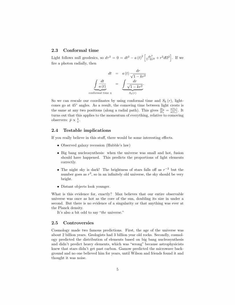
2.3 Conformal time

Light follows null geodesics, so dτ2 = 0 = dt2 − a (t)2[

dr2

1−kr2 + r2dΩ2]. If we

fire a photon radially, then

dt = a (t)dr√

1− kr2dt

a (t)︸ ︷︷ ︸conformal time η

=

dr√1− kr2︸ ︷︷ ︸Sk(r)

.

So we can rescale our coordinates by using conformal time and Sk (r), light-cones go at 45 angles. As a result, the comoving time between light crests isthe same at any two positions (along a radial path). This gives δt2

δt1= a(t2)

a(t1) . Itturns out that this applies to the momentum of everything, relative to comovingobservers: p ∝ 1

a .

2.4 Testable implications

If you really believe in this stuff, there would be some interesting effects.

• Observed galaxy recession (Hubble’s law)

• Big bang nucleosynthesis: when the universe was small and hot, fusionshould have happened. This predicts the proportions of light elementscorrectly.

• The night sky is dark! The brightness of stars falls off as r−2 but thenumber goes as r3, so in an infinitely old universe, the sky should be verybright.

• Distant objects look younger.

What is this evidence for, exactly? Max believes that our entire observableuniverse was once as hot as the core of the sun, doubling its size in under asecond. But there is no evidence of a singularity or that anything was ever atthe Planck density.

It’s also a bit odd to say “the universe.”

2.5 Controversies

Cosmology made two famous predictions. First, the age of the universe wasabout 2 billion years. Geologists had 3 billion year old rocks. Secondly, cosmol-ogy predicted the distribution of elements based on big bang nucleosynthesisand didn’t predict heavy elements, which was “wrong” because astrophysicistsknew that stars didn’t get past carbon. Gamow predicted the microwave back-ground and no one believed him for years, until Wilson and friends found it andthought it was noise.

5

2.6 Angular diameter distance and luminosity distance

Classically, brightness Φ = L4πd2 and ∆θ ≈ D

d . In the FRW metric, dL (z) anddA (z) change. In GR, the angular diameter distance is affected by curvatureand by the change in size of the universe.

Suppose we look at something far away that subtends an angle ∆θ. Wecompute

d⊥ = √

−dτ2

=a (t) rdθ

= a (t) r∆θ= dA∆θ.

This is useless because we don’t know what a (t) or r is for anything we look at.We can apply the Friedman equation (using the convention k = ±1):

ρ = Ωtotρ∗ = (1− Ωk) ρ∗ = (1− Ωk)3H2

8πG

H2 = H2 −H2Ωk −kc2

a2

Ωk =(cH−1

a

)2

k

≈ −k(

radius of horizonradius of curvature

)2

a0 = ±√− k

ΩkcH−1 = cH−1 |Ωk|−1/2

We can then write a (z) = a01+z . Using the definition of conformal time,

∆η =dt

a=

dt

dada

= |Ωk|1/2

H0

H (z)dz︸ ︷︷ ︸

γ

γ = [

ΩΛ + Ωk (1 + z)2 + Ωm (1 + z)3 + Ωγ (1 + z)4]−1/2

dz

r = Sk (∆η)

dA =a0

1 + zSk (∆η) =

cH−10 |Ωk|−1/2

1 + zSk

(|Ωk|

1/2γ)

=cH−1

0

1 + z

Sk

(|Ωk|

1/2γ)

|Ωk|1/2

6

The incoming flux Φ = L4πd2

Lwhere dL is the luminosity distance. But in

GR, we’re affected by the redshift as well as the decrease in the rate at whichphotons arrive. The result is

dL (z) = dA (z) (1 + z)2.

We can use the luminosity distance to probe the expansion history of theuniverse by looking at type 1A supernovae.

Using baryon acoustic oscillations, we determine that there’s extra correla-tion of galaxy positions at a scale of 150Mpc. We can find these correlationsand use them to compute dA. We can do the same thing to the microwavebackground.

3 Inflation

3.1 The horizon and flatness problems

The air in the room we’re in is homogenous, which is fine, because the air onone side of the room is in causal contact with the air on the other side of theroom. But if we plot conformal time, we can see things now that were neverin causal contact (if t = 0 is close to the CMB last scattering surface). Fora ballpark estimate, the horizon is at ct ∼ cH−1 ∼ 3GPc. This is called thehorizon problem.

If we have ρ ∼ a−3 or a−2, then we expect curvature to dominate afterawhile in the expanding universe. If ρ ∼ 1, then the other stuff should dominate.Mathematically, |Ωk| =

(ac

)−2. Depending on the content of the universe,

|Ωk| ∝

a2 if radiation-dominateda if matter-dominateda−2 if vacuum-dominated

.

Suppose the universe were RD at the Planck time 10−43 seconds and becameMD at t ∼ 1012 seconds. Then, during the RD phase, |Ωk| ∝ a2 ∝ t and grewby a factor of 1055. Suring the matter dominated phase, |Ωk| ∝ a and grew bya factor of 3000 or so. We need |Ωk| . 10−60 at the Planck time. This is calledthe flatness problem.

If the expansion history (ρ vs. a) crossed the line for curvature-dominationthat goes through the current state, then things that are in causal contact nowwere in causal contact at the beginning as well.

3.2 Inflation with a scalar field

We need to produce some kind of stuff that doesn’t dilute. We begin with theFriedman equation and drop the curvature term because it becomes negligible

7

quickly. (This is an attractor solution.) We define m = mplanck√8π

, where mplanck =√~cG . ~ = 1 for these purposes.

H2 =8πG

3ρ− kc2

a2=

ρ

3m2

Now we declare that

φ+ 3Hφ+ V ′ (φ) = 0.

The field has units of mass. By looking at the Lagrangian (what Lagrangian?),

ρ =12φ2 + V (φ)

p =12φ2 − V (φ) ,

and w = pρ =

12 φ

2+V (φ)12 φ

2−V (φ)→ −1. The damping happens because the universe is

expanding and tends to damp out relative motion. (It’s a scalar, though, andthere is no obvious relative motion.)

We call the approximation that the field is overdamped the “slow roll” ap-proximation. This means that we can ignore the φ term and the kinetic energydensity term 1

2 φ2. This gives

H2 =ρ

3m2=V (φ)3m2

φ = −V′ (φ)3H

.

To simplify it even more, we define the “number of e-foldings” N ≡ ln(aenda

).

Then dN = −d ln a = −Hdt. Then

dφ

dN= − dφ

Hdt= − φ

H=V ′ (φ)3H2

= m2V′ (φ)

V (φ)

or, in general multifield inflation,

dφ

dN= m2∇ lnV.

To determine when the slow-roll approximation fails, we define two param-

eters ε ≡ m2

2

(V ′

V

)2

and η ≡ m2 V ′′

V which need to have magnitudes smallcompared to unity. During slow roll, we have

N =1m2

V (φ)V ′ (φ)

dφ.

8

3.3 Interpretation of the potential V (φ)

In the (local) homogenous and isotropic approximation, we have a functionφ (~r, t) which does not depend on ~r. A constant V never stops inflating. Alinear V hits zero and bad things happen.

The next simplest one is V (φ) = m2φ2, which works pretty well. The firstslow roll parameter is

ε ≡ m2

2

(V ′

V

)2

=m2

2

(2φ

)2

=2m2

φ2

and inflation ends when φ ∼ φend =√

2m when the kinetic energy of the fieldbecomes significant. The second is

η ≡ m2

∣∣∣∣V ′′V∣∣∣∣ =

2m2

φ2

which gives the same result. The number of e-foldings is

N = − 1m2

φend

φ

V

V ′dφ =

φ2 − φ2end

2m2

andφ (N) =

√φend + 4m2N =

√2m√

1 + 2N.

3.4 Evidence for inflation

There are multiple approaches to measuring h and the Ω parameters and theyare all consistent with the predictions from inflation. The physically meaningfulquantity is ρ

ρend= 1 + 2N , which has no m. To match the CMB fluctuations,

we’d have to be around 10−3 of the Planck scale. These are all calculated forφ when the horizon was the same size it is now. This will become more clearwith the problem set and later lectures. (Problem set hint: ns ≈ 1− 2

N ≈ 0.96.)Inflation would also produce gravitational waves which we can potentially see.These have wavelengths comparable to the horizon and they should imprint asignal on the polarization of the microwave background.

The parameter w = pρ is based on the idea that we don’t know what dark

energy is. If we assume it follows a power law, then w is constant and we canfit it. The result is consistent with −1.

3.5 Crazy effects of inflation

3.5.1 The landscape view

String theory apparently predicts a whole landscape of possible local theoriesdepending on what minimum of whatever fields we’re sitting in. As an example,if we have some wavy potential for a single scalar field, we might have slow-roll

9

inflation forever, inflation followed by recollapse, etc. It turns out that variousinflation models make testable predictions, and some are wrong (e.g. φ4).

Parallel universes are not a theory but predictions of certain theories. If youbelieve in inflation, then you should believe in all of its predictions.

It turns out that slow-roll inflation is forbidden in the most clearly under-stood class of compactifications of string theory.

In any landscape, inflation takes those bits that can inflate and makes thembig, so they actually happen.

3.5.2 Eternal inflation

Inflation generically goes on forever. Most of the universe could get stuck in alocal minimum and then inflation could end by quantum tunneling. The partwhere inflation continues grows faster than it decays away.

If you start with an FRW metric stuck in a local minimum, then any comov-ing bit will eventually “decay” and stop inflating but the bits in between gainvolume even faster.

It turns out that if you just have a local maximum, then the bit on top willinflate for so long that the total (physical) volume increases without bound.When inflation ends, the coordinates tilt so that infinite space comes from whatused to be the infinite time coordinate.

Even φ2 inflates eternally. The inflaton field jiggles a little due to quantummechanics and it turns out that the total volume where you shift up can increasefaster than slow roll eliminates it. There’s a boundary called the quantumdiffusion boundary above which you are driven up more than down. Below thatare the slow roll and reheating regimes.

3.5.3 Measure problem and the A-word

Suppose we want to compute the probability that a random proton has someparameters. If we knew the prior distribution (i.e., what a randomly-chosen pro-ton would be) and the probability that a randomly selected proton end up beingin one of us conditioned on its parameters, we could compute the a posterioridistribution of what we should expect to see.

We get f (p) ∝ fprior (p) fpeople here (p). Both factors are hard to compute,but we cannot ignore the second one.

Suppose we want to compute the probability with which some numbers havethe values they are observed to have. There are few reasons they could have thevalues they have. For example, we don’t expect the Lagrangian of nature to letus compute the mass of earth or the semimajor axis. We’d like to think that theLagrangian would let us compute the mass of the electron and the Bohr radiusof the hydrogen atom.

There are a few parameters that predict most things: α, the fine structureconstant; β, the ratio of electron and proton masses, and mp, the proton mass inPlanck units. These are somewhat coarsely-tuned—bad things happen if they’remuch different. But there is other fine-tuning: we need the neutron to be heavier

10

than the proton, but not much heavier—otherwise the neutron wouldn’t bestable in a nucleus, either. This is due to detailed differences between the quarkmasses, which requires a rather precise Higgs VEV (in those models, anyway).Factors of order unity blow everything up. Even smaller changes dramaticallyalter the carbon and oxygen yield in stars.

3.6 Reheating

During inflation, the energy density of the universe is dominated by the potentialenergy of the field. Once slow roll ends, it turns out that ρ ∝ a−3, just likeordinary matter. Somehow, the energy left over from inflation must have turnedinto other stuff. The details of how this works is unknown.

4 Big bang nucleosynthesis

4.1 Basics

Looking backwards in time, the universe was a lot hotter and denser than it isnow, and far enough back (even before the last scattering surface), it would havebeen as hot as in the core of the sun, so nuclear fusion should have happened.It would be a short-lived process because the universe was expanding, so there’sa nonequilibrium system to solve. George Gamow did a simple approximationof it and got a result rather close to the modern answer. The amount of heliumyou end up with depends on only one number, the baryon-to-photon ratio. andit does not depend very strongly. You can measure that ratio from the CMBand compute the abundances of deuterium, helium, helium-3, and lithium-7.(Gamow thought it was a failure b/c astronomers had said that stars couldn’tmake the heavy elements, which turned out to be wrong. There’s a resonancethat allows three alpha particles to form carbon.)

There is a certain amount of uncertainty in the abundance of stuff, since weneed to correct for post-big-bang nucleosynthesis (in stars), but the error barsare supposed to take that into account and the model seems to work very good.

We know the number and mass density of photons:

nγ =2ζ (3)π2

T 3

ργ =π2

15T 4

We use T from the CMB (now). We find the baryon-to-photon ratio to beη = nb

nγ= 6 · 10−10 (observed). [Note to reader: Max says that no process

after freezeout would have changed η. I don’t see why.] The evolution of theabundances of species is ni = −γini +

∑jk γ

ijknjnk, which is a non-linear stiff

system, but we still know how to solve it. We can approximate this by findingthe very fast processes and assuming that they are always in equilibrium. Some

11

timescales in the problem are Γ = n 〈σv〉, the rate at which a particle interactswith things, and H, the rate at which densities drop due to expansion. Even-tually, the reaction rates drop below the Hubble time and reactions slow down.We can approximate this by equilibrium followed by freezeout.

We start out with the same initial number density of everything, when thetemperature is higher than, say, 1 GeV. We’d expect most of the matter andantimatter to anihiliate at low energy, and, in fact, we’d expect to have evenless left than we have now. The parameter η has no business being a freeparameter—we’d like it to come out of the theory.

4.2 Thermal equilibrium

Some units, first: 1eV = 11604K and 1MeV ∼ 1010K. 1MeV is around thescale of the mass difference between protons and neutrons, the scale of electron-positron pair production, and the scale of nuclear reactions. Therefore, in theearly universe, very little of what’s around depends on historical accidents. Thenumber density at equilibrium is

n (p) d3p =d3p

(2π3)g

eE/kT ± 1,

with E =√m2 + p2, where g depends on the number of degrees of freedom.species g g∗

photon 2 2neutrinos (left-handed) 6 21

4

e+ and e+ 4 72

The density of particles is ρ = 4πn (p)Ep2dp. With m T , we get

g2aBT

4 = π2

30 gT4 for bosons and 7

8π2

30 gT4 for fermions. We define g∗ = 7

8g forfermions, since all we usually care about is the density. The pressure element isp2

3E d3p, so the total pressure is 1

3 the total density. The entropy is S = P+ρT ∝

T 3 ∝ n.Massless particles cool, with T ∝ a−1 (mean energy just redshifts). Con-

servation of entropy per unit comoving volume means that sa3 ∝ g∗T3a3 is

constant.

4.3 Important temperatures

Somewhere around 10MeV, the heavy leptons have decayed and the protons areformed but irrelevent. Neutrinos freeze out around 1MeV (due to the reactionsthat form them becoming slow). Slightly after neutrino freeze-out, big bang nu-cleosynthesis occurs. Protons don’t matter for cosmology until matter-radiationequality, which happens around 1eV / 10000K. Recombination happens around3000K.

• At first, Tγ = Te+ = Tν because of e+ + e− ↔ ν + ν.

12

• Then neutrinos decouple, but the temperatures track each other becausethey cool at the same rate.

• Then the remaning electron-positron pairs annihilate. By conservation ofentropy,

(aT )after

(aT )before=(gbefore∗gafter∗

)1/3

=(

2 + 784

2

)1/3

=(

114

)1/3

.

We can solve this for today’s conditions by

TνTγ

=aTνaTγ

=aT before

γ

aT afterγ

=(

411

)1/3

.

To solve for conditions before matter-radiation equality, we can use

ρradiation = ργ + ρν

ρν =π2

30· 21

4T 2ν = ργ ·

218

(411

)4/3

,

which is a large correction to the number of photons. We can try tomeasure the prefactor to try to count neutrinos. This depends on freezeouttemperatures for hypothetical extra neutrinos, but it still allows somemodels to be ruled out. (The theoretical number of neutrinos is Nν ≈ 3.04due to a little extra heat leaking out into neutrinos.)

4.4 BBN Reactions

n + e+ ↔ p+ + ν

n + ν ↔ p+ + e−

n ↔ p+ + e− + ν

The first two reactions have rate ΛH ≈

(T

0.8MeV

)3. The T 3 comes from

Λ = n︸︷︷︸T 3

〈 σ︸︷︷︸T 2

v︸︷︷︸1

〉. To solve these things, we need to know the cross-sections,

temperatures, and densities. We know the first two, and we know the numberdensity of photons, both before and after BBN. We know the pre-1MeV ratiosof the baryon species, but we don’t know the total number, because the baryonscame from physics we don’t know. The only number we need to find all of theseis η = nb

nγ.

4.5 WIMPs

A WIMP is a weakly interactive massive particle. We can’t have strongly inter-acting massive particles (easy to detect with mass spectroscopy, for example)

13

or electromagnetically interacting massive particles (easy to see). We knowthat dark matter interacts gravitationally, and if the particles are not weaklyinteracting (GIMPs), then we’re screwed.

One redeeming feature of WIMPs is that a simple estimate gives a decentestimate of the amount of dark matter. In Planck units (c = ~ = G = 1), whereξWIMP = m3

WIMPg4T is the density of WIMPs in Planck masses per photon,

〈σv〉 ∼ α2w

Mw

nWIMPS =ρWIMP

MWIMP=

nγξwMWIMP

Annihilation rate Γ ≈ 〈σv〉nWIMP,

giving ξWIMP ∼ 105 v2

g4 ∼ 10−28. This is close to the measured value.

5 The universe to 1st order

Einstein’s equations are nonlinear PDEs and they’re messy to solve directly. Butthe perturbations we have are small, though (initially on the order of 10−5), sowe can linearize and Fourier transform.

5.1 Newtonian analysis

We have three equations.

Conservation of mass ρ+∇ · (ρ~v) = 0

Euler EQ ~v +∇~v = −∇(φ+ p

ρ

)Poisson EQ ∇2φ = 4πGρ

These hold approxmately in GR, too, due to Birkhoff’s Theorem, which saysthat, in sperically symmetric space, things at higher radius don’t matter. So wecan ignore GR.

We now expand around a zeroth-order solution.

ρ0 (t, ~r) = ρ (t) ∝ a−3 if MD

~v0 (t, ~r) =a

a~r

φ (t, ~r) =2πGρ

3r3

The traditional expansion is ρ (t, ~r) = ρ [1 + δ (t, ~r)], ~v (t, ~r) = ~v0 (t, ~r) +~v1 (t, ~r), and φ (t, ~r) = φ0 (t, ~r) + φ1 (t, ~r). When we plug these in, the zeroth-order terms cancel by construction, and we ignore the second-order terms (theyare smaller by five orders of magnitude), so we keep the first-order terms andend up with linear equations.

14

To find ρ, let w ≡ pρ be the equation of state. If we expand a box a little bit,

then thermodynamics says dE = −pdV = −wρdV . Relativity says

dρ = d

(E

V

)=

dE

V− E

V 2dV

= −wρdVV

− ρ

VdV

= −ρ (w + 1) dVd ln ρ = − (1 + w) d lnV

If w is constant, then ρ ∝ V −(1+w) ∝ a−3(1+w).The result is ¨

δ (k) + 2H ˙δ (k) +

(v2sk

2

a2 − 4πGρ)δ (k) = 0. vs is the speed of

sound. In the case of zero pressure, there is no k dependence.In the (inconsistent) case of a static universe, there are oscillatory solutions,

a runaway solution, and a decay solution. The sign depends on whether pressureor gravity wins. The cutoff is k

a =√

4πGρvs

→ λJ = 2πak =

√πGρvs, the Jeans

wavelength. One way to guess this is to compare the τG ∼ 1√Gρ, the timescale

of gravitational collapse with τP ∼ λvs

, the timescale of pressure waves. If thegravitional timescale is smaller, then we have instabilities.

With no curvature and no pressure, we plug in the Friedman equation and getδ+ 2Hδ− 3

2H2δ = 0. This is bizarre—the overdensities do not depend on their

values far away. Assuming a MD universe, H ∝ 23 t−1, so δ+ 4

3 t−1δ− 2

3 t−2δ = 0.

Making the ansatz δ = Atn and solving the resulting quadratic equation givesn = − 1

6 ±56 ∈

−1, 2

3

. So δ ∝ a or δ ∝ a−3/2, and there is a growing mode and

a decaying mode. The decaying mode decays away, so the moral of the story is

δ ∝ a.

This is modified by a few things. First, modes larger than the horizons don’tamplify because no information propagates. Second, in a radiation-dominateduniverse, amplificaiton behaves differently. Before matter-radiation equality,fluctuations don’t grow much. After matter-radiation equality, growth speedsup. Finally, when δ ∼ 1, nonlinear effects prevail.

5.2 Measuring the power spectrum

We imagine the variance of something being related to some distribution. Butthe universe we isn’t a random variable—it’s a single instance of one. It turnsout the entire probability distribution for the overdensity is characterized by asingle function of a single variable.

A Gaussian random vector is a vector with joint density

f (~x) =1

(2π)1/2 |C|1/2

exp(−1

2(~x− ~µ)T C (~x− ~µ)

).

15

Because the harmonic oscillator ground state is a Gaussian, we expect a Gaus-sian distribution for the overdensity.

We can characterize the distribution for an arbitrary random field by givingthe entire family of n-point functions

fn (δ (~r1) , . . . , δ ( ~rn)) ,

which depend only on the mean and covariance. For the overdensity, we’ve de-fined the mean to be zero. The second moment Cij = 〈δi, δj〉 = 〈δ (~ri) , δ (~rj)〉 =ξ (|~ri − ~rk|) because the universe is homogenous and isotropic.

We define the Fourier-space overdensity

δ (~r) =1

(2π)3

ei~k·~r δ

(~k)d3~k

δ(~k)

=ei~k·~rδ (~r) d3~r⟨

δ(~k)∗δ(~k′)⟩

= (2π)3δ(~k − ~k′

)e−i~a·

~kξ (~a) d3a

(2π)3δ(~k − ~k′

)ξ(~k),

et voila! P(~k)

= ξ(~k)

is called the power spectrum. Integrating out the angu-

lar part gives a decomposition by spherical Bessel functions P (k) .=∞

0ξ (r) j0 (kr) dr.

There’s a dimensionless version that is the same in all books ∆2 (k) = 4π(2π)3 k2P (k).

If X is the average overdensity with some window function w (k), then⟨X2⟩

=∆2 (k) |w (k)| d ln k. So ∆2 gives the variance if smoothed out on a scale of k.

(Yes, this is vague. Maybe I’ll fix it.)

6 The transfer function T (z, k)

6.1 Multi-component perturbation growth

The universe contains a number of types of things.

Neutrinos They have a little mass, so they’re significant until VD (around now).

CDM Cold dark matter didn’t matter much until matter-radiation equalitybut matters a lot until VD.

Dark energy Irrelevant until around now.

Normal matter After recombination, they were like CDM. But before recom-bination, there was a photon-baryon fluid, which could have doneweird things between matter-radiation equality and recombination.This fluid’s pressure was dominated by photons (so the speed ofsound was around c√

3) but its density had important contributions

from both.

16

Photons After recombination, they stream freely, but their density doesn’tmatter for very long.

Because there are multiple components, they each feel only their own pressure,but they feel gravity from each other. The new equation is

δi + 2a

aδi + (ci)

2k2δi − 4πG

∑j

ρjδj = 0.

In the matter-dominated era, δ ∝ a. In the VD late universe, growth stops.In the the RD era, most of the energy was in photons, which wouldn’t noticedark matter clumping. In the photon-baryon fluid, λJeans ∼ λhorizon, so nogrowth.

We can solve the rolloffs analytically. For RD and MD, G = 1 + 32aaeq

.

In the late universe, if we define x ≡ ρRρM

= ΩΛΩM

(1 + z)−3 ∝ a3, then GΛ (x) =

56

√1 + 1

x

x0

dy

y1/6(1+y)3/2 , which is reasonably well approximated by x1/3[1 +

(xG3∞

)α]− 13α

,

where α ≈ 0.795 and G∞ =5Γ( 2

3 )Γ( 56 )

3√π

≈ 1.437. So we get an extra ∼ 44% ofgrowth during VD and an extra 5

2 during RD. By matching and combining the

approximations, we get G (x) = 1 + 32x− 1

3eq GΛ (x).

In the photon-baryon fluid, there were driven oscillations, and then, aroundrecombination, something called Silk damping happened that destroyed many ofthese fluctuations, a result of the fact that recombination wasn’t instantaneous—there was a period where the mean free path of the photons is long but notinfinite.

The horizon scale aH ∝ ct ∝ (1 + z)−3/2 when matter dominated. Thephysical wavelength ap ∼ λ

1+z . A mode enters the horizon when aH = ap ⇐⇒

(1 + z)−3/2 ∝ λ1+z . Then 1+zentry ∝ λ−2 ∝ k2. δ ∝ ∆ = ∆enter

1 + zenter if zenter < zeq

1 + zeq otherwise.

So ∆ increases like k2 up to some value keq, when it flattens out. (∆2 ∝ k3p).Clarification: ∆, P , and G are not random. δ is random. G is how much

the mode gets multiplied by, once it’s in the horizon. The power spectrum atany time can be factored P (k, z) = P∗ (k)G (k, z)2, where P∗ is the very earlyuniverse power spectrum, and G is the amplification part.

6.2 Neutrinos

The effect of neutrinos is to suppress the growth of fluctuations on a small scale.There is a characteristic scale; well above the scale there is no suppression andwell below it there is suppression by a constant factor. The scale depends onthe neutrino mass.

If only a fraction Ω∗ of the matter can cluster, then growth decreases toδ ∝ ap, where p =

[√1 + 24Ω∗ − 1

]/4 ≈ Ω3/5

∗ ≈ (1− fν)3/5.

17

Neutrinos don’t cluster on small scales, because they are above the escapevelocity of a clump. The net growth today is ∼ 4700p ≈ 4700e−4fν , so thepower suppression P (k) /P (k)no neutrinos ∼ e−8fν . fν =

∑mν

i/94.4eV ωdm.Neutrinos can be distinguished from curvature or dark matter in that they

actually change the shape of the curve. With enough resolution, the masses ofall three species of neutrinos could be read off.

7 The cosmic microwave background

7.1 Observations

Because we’re looking at the inside surface of a sphere, we decompose the tem-perature in spherical harmonics:

δT

T(r) =

∞∑l=0

l∑m=−l

almYlm (r) .

We expect isotropy, so 〈a∗lmal′m′〉 = δll′δmm′cl, where cl is the variance. Thenormalization gives

δTlT≡√l (l + 1)

2πcl.

To estimate the variance, one way is to look at the values for each m, whichare uncorrelated, and use the usual variance estimator. With a perfect detector,∆clcl

=√

22l+1 .

John Mather showed that the CMB was, in fact, a blackbody. COBE took7 degree resolution pictures at three frequencies.

After COBE, people took higher-resolution pictures from high-altitude bal-loons.

WMAP measures the difference between one position and another position60 degrees away. Then they invert the matrix.

It turns out that the polarization of the CMB might be very interesting.This is difficult to measure, because the polarization signal is around 1% ofthe fluctuations, and the synchotron emission from the galaxy may be stronglypolarized.

7.2 The CMB fluctuation formula∆TT

(r) = φ (~r)− r · ~v (~r) +13δ (r)

In this equation, |~r| is the distance to last scattering.Why are there fluctuations? There are three answers. The photons are

redshifted on the way out of clumps. There is a Doppler effect due to velocities.The density of photons is ρ ∝ T 4, so overdense clumps are hotter.

18

Why are there wiggles? The first bump (around 0.5) is due to the speed ofsound—there are sound waves flying around. The scale is just the horizon sizeat recombination.

What we actually see is a combination of:

• Primary (Effects from z & 103)

– Gravity, doppler, and density (above)

– Damping

– Topological defects, maybe

• Secondary

– Gravity

∗ Early integrated Sachs-Wolfe effect (ISW)∗ Late ISW∗ Rees-Sciama effect∗ Lensing

– Reionization

∗ Local (SZ)· Thermal· Kinematic

∗ Global· Suppression· New doppler· Ostriker-Vishniac

• Tertiary

– Foregrounds

– Headaches

If the universe is MD and linear, then φ = 0. This means that secondaryredshifting due to gravity doesn’t happen unless MD or linearity is violated.Sachs and Wolfe derived a formula δT

T =φ (~r(t)) dt. The early ISW effect is

due to radiation, and the late ISW effect is due to dark energy or curvature. Thelate ISW only started to matter recently, so it would affect the largest scales.The early ISW boosts the first peak, because that was around the horizon sizeat last scattering.

Rees-Sciama is φ due to structure formation. This shows up at the angularscale of nonlinear structures. In practice, this is a couple of orders of magnitudedown from the primary signal, and no one has seen it.

CMB lensing tends to smooth out the power spectrum.

19

There are also projection effects due to the fact that the power spectrumis 3D but we’re looking at a spherical surface. The reinization surface wasn’tperfectly sharp, so the last scattering surface has some approximately Gaussianwidth, which smooths the 2D map and smooths it in the radial direction. Thisis a low-pass filter and kills off the high-frequency components. The scale of thisis around the thickness of the last scattering surface.

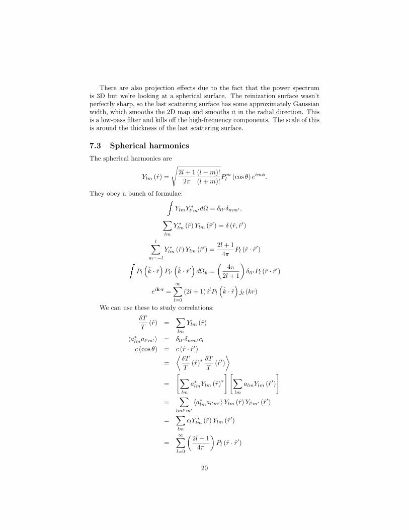
7.3 Spherical harmonics

The spherical harmonics are

Ylm (r) =

√2l + 1

2π(l −m)!(l +m)!

Pml (cos θ) eimφ.

They obey a bunch of formulae:YlmY

∗l′m′dΩ = δll′δmm′ ,∑

lm

Y ∗lm (r)Ylm (r′) = δ (r, r′)

l∑m=−l

Y ∗lm (r)Ylm (r′) =2l + 1

4πPl (r · r′)

Pl

(k · r

)Pl′(k · r′

)dΩk =

(4π

2l + 1

)δll′Pl (r · r′)

eik·r =∞∑l=0

(2l + 1) ilPl(k · r

)jl (kr)

We can use these to study correlations:

δT

T(r) =

∑lm

Ylm (r)

〈a∗lmal′m′〉 = δll′δmm′cl

c (cos θ) = c (r · r′)

=⟨δT

T(r)∗

δT

T(r′)⟩

=

[∑lm

a∗lmYlm (r)∗][∑

lm

almYlm (r′)

]=

∑lml′m′

〈a∗lmal′m′〉Ylm (r)Yl′m′ (r′)

=∑lm

clY∗lm (r)Ylm (r′)

=∞∑l=0

(2l + 1

4π

)Pl (r · r′)

20

7.4 Projection effects

The effect of a source being in a gravitational well is the redshift, giving δTT = φ,

except that things in a gravitational well cool more slowly (due to time dilation),which means it’s hotter, which has the opposite sign. T ∝ a−1 ∝ t−2/3, soδTT = − 2

3δTT = − 2

3φ, giving an actual contribution of

δT

T=

13φ.

Now we write

δT

T(r) =

13φ (r)

=13

1(2π)3

eik·rφ (k) d3k

c (r · r′) =

⟨19

1(2π)6

[e−ik·rφ∗ (k) d3k

] [eik′·r′ φ∗ (k′) d3k′

]⟩

=19

1(2π)6

e−ik·reik

′·r′⟨φ∗ (k) φ (k′)

⟩︸ ︷︷ ︸

=(2π)3δ(k−k′)Pφ(k)

d3kd3k′

=19

1(2π)3

(eik·r

)∗eik·r

′Pφ (k) d3k

=19

1(2π)3

[∑l

(2l + 1) (−i)l Pl(k · r

)jl (kr)

][∑l′

(2l′ + 1) ilPl(k · r′

)jl (kr)

]k2dkdΩ

=19

1(2π)3

∑l

(2l + 1)2jl (kr) jl (kr′)

4π2l + 1

Pl (r · r′)Pφ (k) d2dk

=19

(4π)2

(2π)3

∑l

(2l + 1)4π

jl (kl)2Pφ (k)Pl (r · r′) k2dk

cl =19

(4π2)

(2π)3

jk (kl)2

Pφ (k) k2dk

This gives the expected spherical harmonic power as a function of the 3Dpower spectrum.

7.5 Nonlinear effects

When the linear theory predicts an overdensity of ˜1.69, the nonlinear theorypredicts infinite density, which means that the clump “virializes” and forms abound object with density around 200 times the background.

The Press-Schechter approximation says that a point is in a virialized haloof mass exceeding M if an appropriately smoothed δ at that point exceeded 1.69at the appropriate time, which gives something like erfc

[δc

σ(M,z)

], which grows

21

very quickly as the number of sigmas changes. The trouble with interpretingthis data is figuring out the mass. We can now look at the clusters in visiblelight, X-rays, lensing, etc.

7.6 Seeing other effects

7.6.1 ISW

We now see the late ISW effect at respectable significance. We can’t see theRees-Sciama effect yet.

7.6.2 Global reionization

Plasma due to reionization scatters light. We parameterize it by the reioniza-tion optical depth τ =

σTnedx. This washes out large-l power. (For l 10,

cl ∼ cle−2τ .) For smaller l, there is little effect. There is some increase at

medium scales due to fluctiations in the plasma. There’s some annoyance be-cause changing the seed fluctuation size and τ only affects small l in a mannerthat’s somewhat degenerate with the ISW.

The OV (Ostriker-Vishniac) effect is a second-order effect during reionizationthat may be apparent at very small scales (l ∼ 104). It’s like a kinetic SZ effectcaused by general diffuse hydrogen.

7.6.3 Local reionization

The thermal SZ effect occurs because galaxy clusters contain hot gasses, ataround 5-15keV. This changes the spectrum by heating some cold photons. It’sdetectable by the frequency spectrum of the CMB. It’s a suppression belowV∗ = 217GHz and an amplification above. (V∗ is called the SZ null frequencyand is a small multiple of the CMB temperature. Relativistic gasses can perturbit 1-2MHz higher.) The suppression in antenna temperature asymptotes to aconstant at low frequency (i.e. constant decrease in T). At higher frequencies,∆T ∝ V − V∗.

The strength of the SZ effect is independent of cluster redshift, so we canfind all clusters by looking for holes in the CMB.

Galaxy clusters are also moving, which causes them to Doppler shift theCMB, about 10 times less than the thermal SZ effect. We can use this tomeasure the radial velocities of the clusters by changes at the SZ null frequency.(This is the same physics as the Ostriker-Vishniac effect.)

7.7 CMB polarization

The last thing that the CMB light did before reaching us was to Thompsonscatter off an electron. Thompson scattering is highly polarizing, but this ef-fect is neutralized because light hits scattering electrons from all directions. Ifthere is quadrupole anisotropy in the CMB, though, there will be some residualpolarization.

22

7.8 Measuring the CMB

At low frequencies (˜23GHz), we see synchotron radiation from the galaxy. Athigh frequencies, we see blackbody emission from dust in the galaxy.

The WMAP team’s approach to removing this foreground is to take a linearcombination of the five maps (at different frequencies) that minimizes totalpower. If the weights are allowed to depend on the multipole moment, then youcan do better, because different types of foregrounds are dominant at differentangular scales.

Polarization is harder because the signal is weaker and the foregrounds arestronger (e.g. synchotron radiation could be 70% polarized).

The polarization field can be decomposed into T, E and B modes (related tothe angle between the polarization and the gradient). This gives three scalars.The power spectra and cross-power spectra can be measures (it turns out thatthe cross-power that can be nonzero is TE). B is not expected to be amplifiedduring expansion, but inflation can produce B modes. The Sachs-Wolfe effectin particular does not polarize at all.

8 Lensing

Gravity bends light. If we see a point source lined up with a point mass, it’llshow up as a ring, and, if it’s a little off, we’ll see an arc and some points instead.Farther out, things look more elliptical than they are. If we look far away andsee correlated ellipticities, then this might indicate dark matter (it turns outthat nearby galaxies might have correlations due to tides).

Lensing has the property that the surface brightness (flux per unit solidangle) never changes.

In this section, unprimed coordinates are pre-lensing, and primed coordinatesare what we see in the presence of lensing.

F ′ =φ′(~θ′)d2~θ′

=φ′(~θ′)

∣∣∣∣∣d~θ′d~θ∣∣∣∣∣ d2θ

The Jacobian is nearly constant over the support of the flux (i.e. the size of thegalaxy), so

F ′ = F |J| .

This is annoying because we don’t know F in general. We could do a similarcalculation for the position shift, but we have the same problem because wedon’t know where the source really is.

If we define f (θ′) =φ(θ′)F to be the normalized density of where the light

comes from, then the second moment is the quadrupole (covariance) Q =

23

⟨(~θ −

⟨~θ⟩)(

~θ −⟨~θ⟩)T⟩

. We can linearize the mapping, giving ~θ′ =⟨~θ′⟩

+

J(~θ −

⟨~θ⟩)

. The quadrupole simplifies to Q′ = JQJT . We assume that the

universe is isotropic, even in a particular direction, so 〈Q〉galaxies = σ2I. Thetransformation of the quadrupole is linear, so 〈Q′〉galaxies = σ2JJT .

One way to relate this to the physics is by the time delay τ ∝ 12

(~θ′ − ~θ

)2

−ψ (θ) where ψ (θ) is the gravitational time delay. With multiple images, we canmeasure this directly. But with Fermat’s principle, there is an image where 0 =∇τ = ~θ′−~θ−∇ψ ⇐⇒ ~θ′ = ~θ∇ψ. The Jacobian is thus Jij = δij+ψ,ij = I+M,where M is the Hessian. This means that the Jacobian matrix is symmetric, and

we can parameterize it as J =(

1 + κ+ γ1 γ2

γ2 1 + κ+ γ1

). κ is the convergence

and the γ’s are the shears. The magnification is J = (1 + κ)2−γ1−γ2. In weaklensing, these numbers are small, so J ≈ 1 + 2κ.

From now on, φ is Newtonian gravitational potential.In Euclidean space, δ~θ =

A (r)∇⊥φdr. A (r) is a slowly varying geometri-

cal factor, and, if the lensing is caused by a galaxy cluster at a narrow range ofz, δ~θ ≈ ∇⊥

(A (r)

φdr

)= ∇⊥ψ.

We can now relate lensing to density (Σ is the surface density of the cluster):

∇2⊥ψ = A

(∇2 − ∂2

r

)φdr

∇2φdr =

4πGρdr = 4πGΣ

∂2rφdr = φ′ (rmax)− φ′ (rmin) = 0.

So 1 + κ = 12 Tr J = 1

2∇2⊥ψ = 1

2ΣΣ2 .

After accounting for the expanding universe and other such details, the powerspectrum of κ is Pκ (l) =

(32ωmc

)2 ηhor

0W (η)2

P(

lSk(η) , z (η)

)(1 + z (η))2

dη,

where W (η) = ηhor

ηG (η′)

Sk(η′−η)Sk(η′) dη′ and G (η) is the distribution of source

redshifts, and the popular fit is G (η) = B

z0Γ( 1+αB )

(zz0

)αexp

[−(zz0

)β]. The

good news is that it shows the location of all matter as opposed to just baryonicmatter. The bad news is that there are nonlinear growth effects, blobs of gas, andother stuff. There is also a problem in that anisotropic point spread functions intelescopes looks just like lensing, so some corrections are needed. These effectsare large but can be corrected with care. It turns out that you can even dolensing tomography if you measure each galaxy’s redshift individually.

24

9 The Lyman α forest

If we look at a distant quasar, the absorption due to the (redshifted) Lyman αline from neutral hydrogen in the way gives a map of density along that line.There are some issues due to Doppler broadening (temperature-dependent) andionization, but it has good sensitivity on small scales. The best data is fromSDSS, which has spectra for about 105 quasars, and the Keck high-res spectra,which has fewer quasars.

10 21-cm tomography

We would like to measure the density field δ in the observable universe. We’vecovered a very small portion of the volume so far. The density ratio of tripletsto singlets is

n1

n0= 3 exp [T∗/Ts]

where T∗ =??. TS is the spin temperature. Early on, the CMB does a goodjob of driving the spin transition, so the spin temperature would be the CMBtemperature and there would be nothing to see. But gas cools faster than light(a−2) once the gas is decoupled enough, so the hydrogen ends up cooling fasterbecause collisions cool it faster than heating from the CMB. As a result, we’ll seeit being colder than the CMB. Once reionization starts, the spin temperaturewill increase due to UV and the hydrogen will heat up dramatically. This meansthat around 9 < z < 50 we’ll see it in absorption and at z < 9 or so we’ll see itin emission. The fluctuation in the brightness temperature is around

δTb ≈ 29mK(hΩb0.03

)(Ωm0.25

)−1/2√

1 + z

10(1 + x) (1 + δ)

(TS − TCMB

TS

)where x is the ionization fraction.

There are all kinds of interesting models to rule out at very small scales.

25