84140183 Feedback Control Systems Lab Manual
141
Feedback Control Systems Laboratory Experiments Handbook College of Electrical and Mechanical Engineering National University of Sciences and Technology
-
Upload
jose-ramon-iglesias -
Category
Documents
-
view
96 -
download
0
Transcript of 84140183 Feedback Control Systems Lab Manual

Feedback Control Systems Laboratory Experiments Handbook
College of Electrical and Mechanical Engineering
National University of Sciences and Technology
2
Supervisor
DR.KHALID MUNAWAR
Course developed by:
MUHAMMAD OVAIS ZUBERI DE25 MECHATRONICS
AAMNA FAYYAZ DE25 MECHATRONICS
3
Contents
LAB1: Introduction to MATLAB and SIMULINK …………………. 5 1. Overview of basic MATLAB environment and features.
a. Vectors
b. Functions
c. Plotting
d. Polynomials
e. Matrices
f. Printing
g. Using Mfiles in MATLAB
h. Getting help in MATLAB 2. The Control Systems Toolbox in MATLAB
3. Basic SIMULINK concepts
a. Starting Simulink
b. Model Files
c. Basic Elements
d. Running Simulations
e. Building Systems
LAB2: Introduction to Laboratory Trainer hardware………………… 37 1. General overview
a. System Nomenclature
b. System Schematics
c. Component Description d. System Parameters
e. Hardware Configuration
2. Setting up the trainer for experiments.
LAB3: Introduction to Laboratory Trainer Software…………………. 49 1. Introduction
2. Getting Started
3. Plots
4. The Signal Generator
LAB4: System Modeling …………………………………………….. 63 1. Introduction
2. Nomenclature
3. Practice first principles modeling
a. Reading Motor datasheets
b. Developing motor transfer functions in MATLAB using the CS toolbox
c. Determining System Parameters
d. Pre-lab results summary table
4. Modeling module graphical user interface a. Module Startup
b. Static Relations
c. Dynamic Models
d. In-lab results summary table
4
LAB5: Speed Control………………………………………………… 81 1. Introduction to the PI controller
a. PI control law (set-point, Kp,Ki)
b. Magic of Integral action
2. Nomenclature
3. Pre-lab assignment
a. PI controller design to given specifications using MATLAB CS toolbox.
b. Tracking triangular signals (power of time input) c. Response to load disturbances
d. Pre-lab results summary table
e. Speed control module graphical user interface
f. Module Description/Startup
4. Qualitative properties of proportional and integral control
5. Manual Tuning using Ziegler-Nichols
a. Design to given specifications
b. Tracking triangular signals (power of time input)
c. Response to load disturbances
d. In-lab results summary table
LAB6: Position Control……………………………………………… 97 1. Introduction to the PID controller
a. PI control law (set-point, Kp, Ki) b. Magic of Integral action
c. Controller with two degrees of freedom
2. Nomenclature
3. Pre-lab assignment
a. Comparison between PD position and PI speed control
b. Fundamental limitations and achievable performance
c. PD controller design to given specifications using MATLAB CS toolbox.
d. Tracking triangular signals (power of time input)
e. Response to load disturbances
f. Pre-lab results summary table
4. Position control module graphical user interface
a. Module Description/Startup b. Qualitative properties of proportional and derivative control
c. Design to given specifications
d. Tracking triangular signals (power of time input)
e. Response to load disturbances f. In-lab results summary table
LAB7: Robust Control……………………………………………...... 118 1. Introduction
2. Nomenclature
3. Pre-lab assignment
a. MATLAB script
b. Robustness and Sensitivity
c. Stability Margins
d. Pre-lab results summary table 4. Robustness module graphical user interface
a. Module Description/Startup
b. stability margin evaluation
c. In-lab results summary table

5
LAB 1
Introduction to MATLAB and SIMULINK
Contents:
Overview of basic MATLAB environment and features. Vectors
Functions
Plotting
Polynomials
Matrices
Printing
Using Mfiles in MATLAB
Getting help in MATLAB
The Control Systems Toolbox in MATLAB
Basic SIMULINK concepts Starting Simulink
Model Files
Basic Elements
Running Simulations
Building Systems

6
MATLAB is an interactive program for numerical computation and data visualization; it is used
extensively by control engineers for analysis and design. There are many different toolboxes available
which extend the basic functions of MATLAB into different application areas; in these tutorials, we will
make extensive use of the Control Systems Toolbox. MATLAB is supported on Unix, Macintosh, and
Windows environments; a student version of MATLAB is available for personal computers. For more
information on MATLAB, contact the MathWorks.
The idea behind these tutorials is that you can view them in one window while running
MATLAB in another window. You should be able to redo all of the plots and calculations in
the tutorials.
Vectors
Let's start off by creating something simple, like a vector. Enter each element of the vector (separated by
a space) between brackets, and set it equal to a variable. For example, to create the vector a, enter into
the MATLAB command window
a = [1 2 3 4 5 6 9 8 7]
MATLAB should return: a =
1 2 3 4 5 6 9 8 7
Let's say you want to create a vector with elements between 0 and 20 evenly spaced in increments of 2
(this method is frequently used to create a time vector): t = 0:2:20
t =
0 2 4 6 8 10 12 14 16 18 20
Manipulating vectors is almost as easy as creating them. First, suppose you would like to add 2 to each
of the elements in vector 'a'. The equation for that looks like: b = a + 2
b =
3 4 5 6 7 8 11 10 9
Now suppose, you would like to add two vectors together. If the two vectors are the same length, it is
easy. Simply add the two as shown below: c = a + b
c =
4 6 8 10 12 14 20 18 16
Subtraction of vectors of the same length works exactly the same way.
Functions
To make life easier, MATLAB includes many standard functions. Each function is a block of code that
accomplishes a specific task. MATLAB contains all of the standard functions such as sin, cos, log, exp,
sqrt, as well as many others. Commonly used constants such as pi, and i or j for the square root of -1, are
also incorporated into MATLAB.

7
sin(pi/4)
ans =
0.7071
To determine the usage of any function, type help [function name] at the MATLAB command
window.
MATLAB even allows you to write your own functions with the function command. More Information
about functions is given at the end of the handbook.
Plotting
It is also easy to create plots in MATLAB. Suppose you wanted to plot a sine wave as a function of time.
First make a time vector (the semicolon after each statement tells MATLAB we don't want to see all the
values) and then compute the sin value at each time. t=0:0.25:7;
y = sin(t);
plot(t,y)
The plot contains approximately one period of a sine wave. Basic plotting is very easy in MATLAB, and
the plot command has extensive addon capabilities. More Information about Plotting is given at the end
of the handbook.
Polynomials
In MATLAB, a polynomial is represented by a vector. To create a polynomial in MATLAB, simply enter
each coefficient of the polynomial into the vector in descending order. For instance, let's say you have
the following polynomial:
To enter this into MATLAB, just enter it as a vector in the following manner
x = [1 3 15 2 9]

8
x =
1 3 15 2 9
MATLAB can interpret a vector of length n+1 as an nth order polynomial. Thus, if your polynomial is
missing any coefficients, you must enter zeros in the appropriate place in the vector. For example,
would be represented in MATLAB as:
y = [1 0 0 0 1]
You can find the value of a polynomial using the polyval function. For example, to find the value of
the above polynomial at s=2, z = polyval([1 0 0 0 1],2)
z =
17
You can also extract the roots of a polynomial. This is useful when you have a high order polynomial
such as
Finding the roots would be as easy as entering the following command;
roots([1 3 -15 -2 9])
ans =
5.5745
2.5836
0.7951
0.7860
Let's say you want to multiply two polynomials together. The product of two polynomials is found by
taking the convolution of their coefficients. MATLAB's function conv that will do this for you. x = [1 2];
y = [1 4 8];
z = conv(x,y)
z =
1 6 16 16
Dividing two polynomials is just as easy. The deconv function will return the remainder as well as the
result. Let's divide z by y and see if we get x. [xx, R] = deconv(z,y)
xx =
1 2
R =
0 0 0 0
As you can see, this is just the polynomial/vector x from before. If y had not gone into z evenly, the
remainder vector would have been something other than zero.
Matrices

9
Entering matrices into MATLAB is the same as entering a vector, except each row of elements is
separated by a semicolon (;) or a return: B = [1 2 3 4;5 6 7 8;9 10 11 12]
B =
1 2 3 4
5 6 7 8
9 10 11 12
B = [ 1 2 3 4
5 6 7 8
9 10 11 12]
B =
1 2 3 4
5 6 7 8
9 10 11 12
Matrices in MATLAB can be manipulated in many ways. For one, you can find the transpose of a
matrix using the apostrophe key: C = B'
C =
1 5 9
2 6 10
3 7 11
4 8 12
It should be noted that if C had been complex, the apostrophe would have actually given the complex
conjugate transpose. To get the transpose, use .' (the two commands are the same if the matrix is not
complex).
Now you can multiply the two matrices B and C together. Remember that order matters when
multiplying matrices. D = B * C
D =
30 70 110
70 174 278
110 278 446
D = C * B
D =
107 122 137 152
122 140 158 176
137 158 179 200
152 176 200 224
Another option for matrix manipulation is that you can multiply the corresponding elements of two
matrices using the .* operator (the matrices must be the same size to do this). E = [1 2;3 4]
F = [2 3;4 5]
G = E .* F
E =
1 2

10
3 4
F =
2 3
4 5
G =
2 6
12 20
If you have a square matrix, like E, you can also multiply it by itself as many times as you like by
raising it to a given power. E^3
ans =
37 54
81 118
If wanted to cube each element in the matrix, just use the element-by-element cubing. E.^3
ans =
1 8
27 64
You can also find the inverse of a matrix: X = inv(E)
X =
2.0000 1.0000
1.5000 0.5000
or its Eigen-values: eig(E)
ans =
0.3723
5.3723
There is even a function to find the coefficients of the characteristic polynomial of a matrix. The "poly"
function creates a vector that includes the coefficients of the characteristic polynomial. p = poly(E)
p =
1.0000 5.0000 2.0000
Remember that the Eigen-values of a matrix are the same as the roots of its characteristic polynomial: roots(p)
ans =
5.3723
0.3723
Using M-files in MATLAB
There are slightly different things you need to know for each platform.

11
Windows
Running MATLAB from Windows is very similar to running it on a Macintosh. However, you need to
know that your m-file will be saved in the clipboard. Therefore, you must make sure that it is saved as
filename.m
Getting help in MATLAB
MATLAB has a fairly good online help; type
help commandname
for more information on any given command. You do need to know the name of the command that you
are looking for. Here are a few end notes for this section.
You can get the value of a particular variable at any time by typing its name. B
B =
1 2 3
4 5 6
7 8 9
You can also have more that one statement on a single line, so long as you separate them with either a
semicolon or comma.
Also, you may have noticed that so long as you don't assign a variable a specific operation or result,
MATLAB with store it in a temporary variable called "ans".
The Control Systems Toolbox in MATLAB
By writing the following command the Graphical User interface of the Control Systems toolbox opens
up: Sisotool

12
The Siso design tool allows users to modify the system compensator parameters in anyway they find
suitable. They can modify the Root loci in the Root locus editor or specify the frequency domain
characteristics using bode or nyquist plots. They can also numerically feed in the compensator and see
its effect on both the root loci and bode/nyquist plots.
By pulling the analysis pulldown menu, they can launch the LinearTimeInvariant Viewer in which they
can view the step and impulse response of system parameters.
The Control Systems Toolbox will be discussed further in all the accompanying sections in this
handbook.
Basic SIMULINK concepts
Simulink is a graphical extension to MATLAB for modeling and simulation of systems. In Simulink,
systems are drawn on screen as block diagrams. Many elements of block diagrams are available, such as
transfer functions, summing junctions, etc., as well as virtual input and output devices such as function
generators and oscilloscopes. Simulink is integrated with MATLAB and data can be easily transferred
between the programs. In these tutorials, we will apply Simulink to the examples from the MATLAB
tutorials to model the systems, build controllers, and simulate the systems. Simulink is supported on
Unix, Macintosh, and Windows environments; and is included in the student version of MATLAB for
personal computers. For more information on Simulink, contact the MathWorks.

13
The idea behind these tutorials is that you can view them in one window while running Simulink in
another window. System model files can be downloaded from the tutorials and opened in Simulink. You
will modify and extend these systems while learning to use Simulink for system modeling, control, and
simulation. Do not confuse the windows, icons, and menus in the tutorials for your actual Simulink
windows. Most images in these tutorials are not live they simply display what you should see in your
own Simulink windows. All Simulink operations should be done in your Simulink windows.
Starting Simulink
Simulink is started from the MATLAB command prompt by entering the following command: simulink
Alternatively, you can hit the New Simulink Model button at the top of the MATLAB command window
as shown below:
When it starts, Simulink brings up two windows. The first is the main Simulink window, which appears
as:
The second window is a blank, untitled, model window. This is the window into which a new model can
be drawn.
Model Files

14
In Simulink, a model is a collection of blocks which, in general, represents a system. In addition, to
drawing a model into a blank model window, previously saved model files can be loaded either from the
File menu or from the MATLAB command prompt. As an example, download the following model file
save the file in the directory you are running MATLAB from. simple.mdl
Open this file in Simulink by entering the following command in the MATLAB command window.
(Alternatively, you can load this file using the Open option in the File menu in Simulink, or by hitting
Ctrl+O in Simulink.) simple
The following model window should appear.
A new model can be created by selecting New from the File menu in any Simulink window (or by
hitting Ctrl+N).
Basic Elements
There are two major classes of items in Simulink: blocks and lines. Blocks are used to generate, modify,
combine, output, and display signals. Lines are used to transfer signals from one block to another.
Blocks
There are several general classes of blocks:
Sources: Used to generate various signals
Sinks: Used to output or display signals
Discrete: Linear, discrete-time system elements (transfer functions, state-space models, etc.)

15
Linear: Linear, continuous-time system elements and connections (summing junctions, gains,
etc.)
Nonlinear: Nonlinear operators (arbitrary functions, saturation, delay, etc.)
Connections: Multiplex, Demultiplex, System Macros, etc.
Blocks have zero to several input terminals and zero to several output terminals. Unused input terminals
are indicated by a small open triangle. Unused output terminals are indicated by a small triangular point.
The block shown below has an unused input terminal on the left and an unused output terminal on the
right.
Lines
Lines transmit signals in the direction indicated by the arrow. Lines must always transmit signals from
the output terminal of one block to the input terminal of another block. On exception to this is a line can
tap off of another line, splitting the signal to each of two destination blocks, as shown below: (open the
model file named split.mdl).
Lines can never inject a signal into another line; lines must be combined through the use of a block such
as a summing junction.
A signal can be either a scalar signal or a vector signal. For SingleInput, SingleOutput systems, scalar
signals are generally used. For MultiInput, MultiOutput systems, vector signals are often used,
consisting of two or more scalar signals. The lines used to transmit scalar and vector signals are
identical. The type of signal carried by a line is determined by the blocks on either end of the line.
Simple Example
The simple model consists of three blocks: Step, Transfer Fcn, and Scope. The Step is a source block

16
from which a step input signal originates. This signal is transferred through the line in the direction
indicated by the arrow to the Transfer Function linear block. The Transfer Function modifies its input
signal and outputs a new signal on a line to the Scope. The Scope is a sink block used to display a signal
much like an oscilloscope.
There are many more types of blocks available in Simulink, some of which will be discussed later. Right
now, we will examine just the three we have used in the simple model.
Modifying Blocks
A block can be modified by double clicking on it. For example, if you double click on the "Transfer
Fcn" block in the simple model, you will see the following dialog box.
This dialog box contains fields for the numerator and the denominator of the block's transfer function.
By entering a vector containing the coefficients of the desired numerator or denominator polynomial, the
desired transfer function can be entered. For example, to change the denominator to s^2+2s+1, enter the
following into the denominator field: [1 2 1]
and hit the close button, the model window will change to the following,
which reflects the change in the denominator of the transfer function. The "step" block can also be
double clicked, bringing up the following dialog box.

17
The default parameters in this dialog box generate a step function occurring at time=1 sec, from an
initial level of zero to a level of 1. (in other words, a unit step at t=1). Each of these parameters can be
changed. Close this dialog before continuing.
The most complicated of these three blocks is the "Scope" block. Double clicking on this brings up a
blank oscilloscope screen.
When a simulation is performed, the signal which feeds into the scope will be displayed in this window.
Detailed operation of the scope will not be covered in this tutorial. The only function we will use is the
auto-scale button, which appears as a pair of binoculars in the upper portion of the window.
Running Simulations
To run a simulation, we will work with the following model file: simple2.mdl
Open this file in Simulink. You should see the following model window.

18
Before running a simulation of this system, first open the scope window by doubleclicking on the scope
block. Then, to start the simulation, either select Start from the Simulation menu (as shown below) or
hit CtrlT in the model window.
The simulation should run very quickly and the scope window will appear as shown below.
Note that the simulation output (shown in yellow) is at a very low level relative to the axes of the scope.
To fix this, hit the auto-scale button (binoculars), which will rescale the axes as shown below.

19
Note that the step response does not begin until t=1. This can be changed by doubleclicking on the
"step" block. Now, we will change the parameters of the system and simulate the system again.
Doubleclick on the "Transfer Fcn" block in the model window and change the denominator to [1 20 400]
Rerun the simulation (hit CtrlT) and you should see what appears as a flat line in the scope window. Hit
the auto-scale button, and you should see the following in the scope window.
Notice that the auto-scale button only changes the vertical axis. Since the new transfer function has a
very fast response, it compressed into a very narrow part of the scope window. This is not really a
problem with the scope, but with the simulation itself. Simulink simulated the system for a full ten
seconds even though the system had reached steady state shortly after one second.
To correct this, you need to change the parameters of the simulation itself. In the model window, select
Parameters from the Simulation menu. You will see the following dialog box.
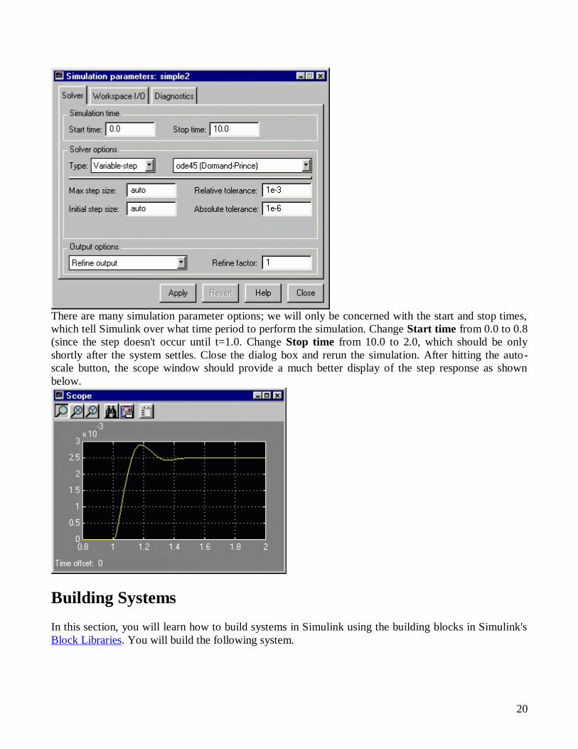
20
There are many simulation parameter options; we will only be concerned with the start and stop times,
which tell Simulink over what time period to perform the simulation. Change Start time from 0.0 to 0.8
(since the step doesn't occur until t=1.0. Change Stop time from 10.0 to 2.0, which should be only
shortly after the system settles. Close the dialog box and rerun the simulation. After hitting the auto-
scale button, the scope window should provide a much better display of the step response as shown
below.
Building Systems
In this section, you will learn how to build systems in Simulink using the building blocks in Simulink's
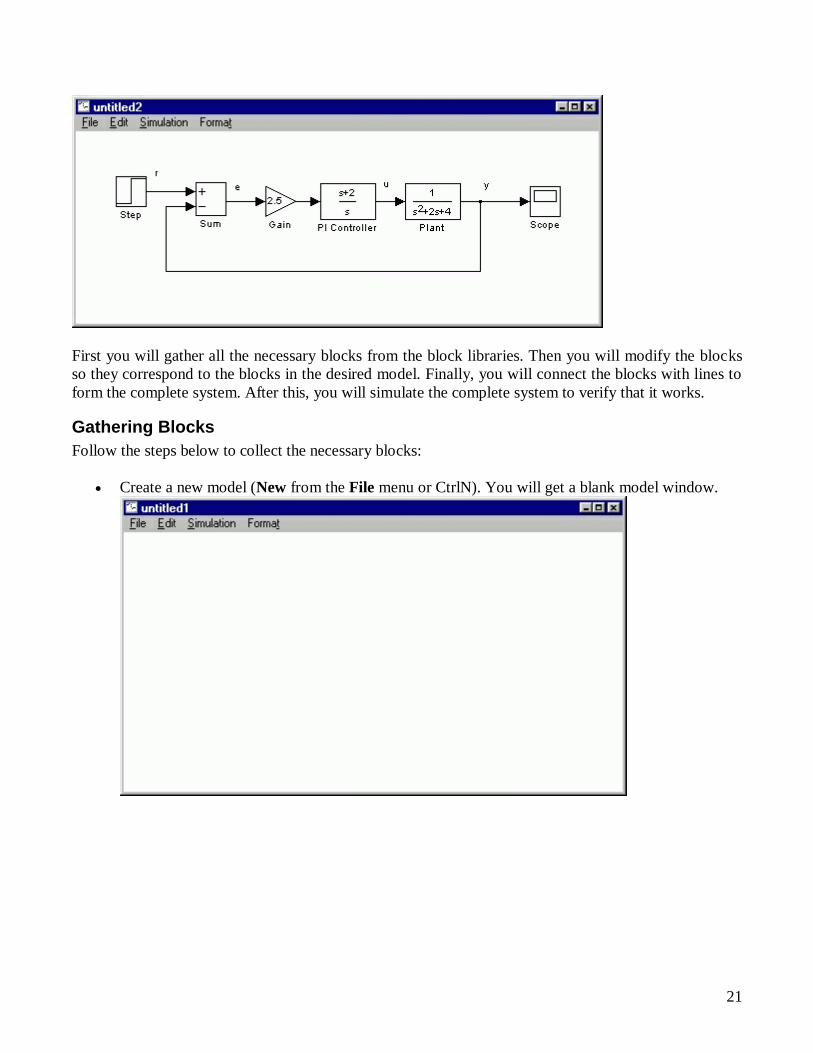
Block Libraries. You will build the following system.
21
First you will gather all the necessary blocks from the block libraries. Then you will modify the blocks
so they correspond to the blocks in the desired model. Finally, you will connect the blocks with lines to
form the complete system. After this, you will simulate the complete system to verify that it works.
Gathering Blocks
Follow the steps below to collect the necessary blocks:
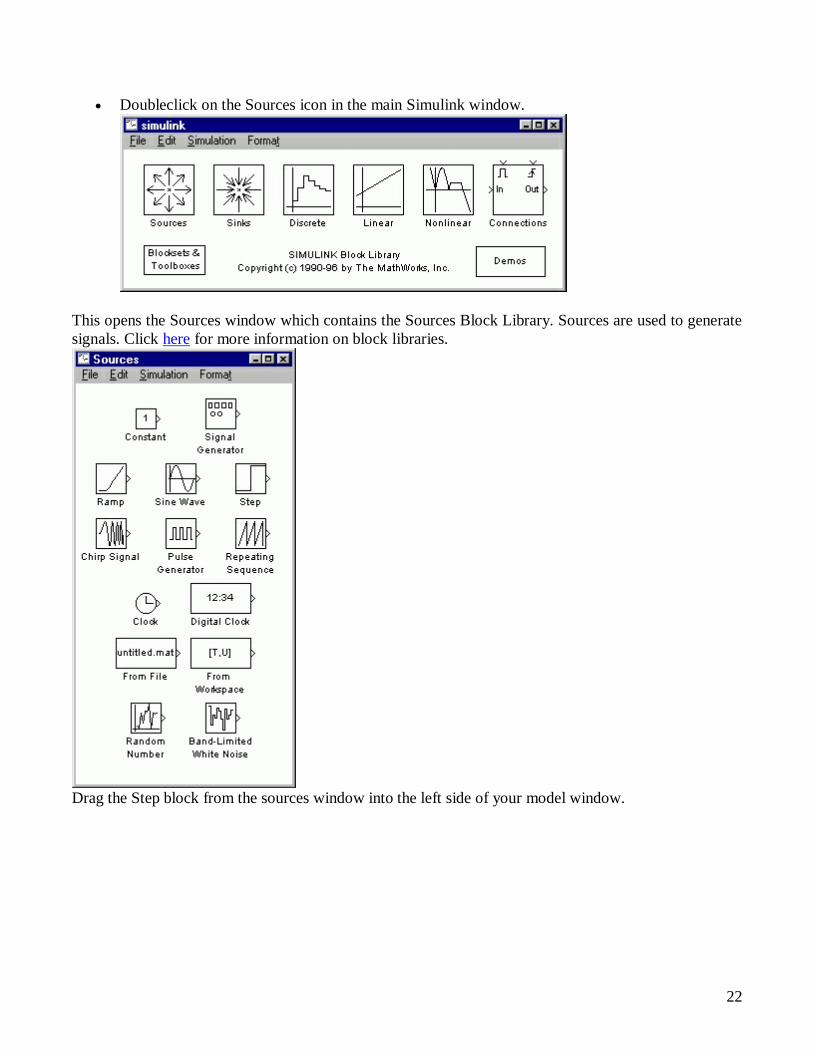
Create a new model (New from the File menu or CtrlN). You will get a blank model window.
22
Doubleclick on the Sources icon in the main Simulink window.
This opens the Sources window which contains the Sources Block Library. Sources are used to generate
signals. Click here for more information on block libraries.
Drag the Step block from the sources window into the left side of your model window.

23
Doubleclick on the Linear icon in the main Simulink window to open the Linear Block Library
window.
Drag the Sum, Gain, and two instances of the Transfer Fcn (drag it two times) into your model
window arranged approximately as shown below. The exact alignment is not important since it
can be changed later. Just try to get the correct relative positions. Notice that the second Transfer
Function block has a 1 after its name. Since no two blocks may have the same name, Simulink
automatically appends numbers following the names of blocks to differentiate between them.
Doubleclick on the Sinks icon in the main Simulink window to open the Sinks window.
Drag the Scope block into the right side of your model window.

24
Modify Blocks
Follow these steps to properly modify the blocks in your model.
Doubleclick your Sum block. Since you will want the second input to be subtracted, enter + into
the list of signs field. Close the dialog box.
Doubleclick your Gain block. Change the gain to 2.5 and close the dialog box.
Doubleclick the leftmost Transfer Function block. Change the numerator to [1 2] and the
denominator to [1 0]. Close the dialog box.
Doubleclick the rightmost Transfer Function block. Leave the numerator [1], but change the
denominator to [1 2 4]. Close the dialog box. Your model should appear as:
Change the name of the first Transfer Function block by clicking on the words "Transfer Fcn". A
box and an editing cursor will appear on the block's name as shown below. Use the keyboard
(the mouse is also useful) to delete the existing name and type in the new name, "PI Controller".
Click anywhere outside the name box to finish editing.

25
Similarly, change the name of the second Transfer Function block from "Transfer Fcn1" to
"Plant". Now, all the blocks are entered properly. Your model should appear as:
Connecting Blocks with Lines
Now that the blocks are properly laid out, you will now connect them together. Follow these steps.
Drag the mouse from the output terminal of the Step block to the upper (positive) input of the
Sum block. Let go of the mouse button only when the mouse is right on the input terminal. Do
not worry about the path you follow while dragging, the line will route itself. You should see the
following.

26
The resulting line should have a filled arrowhead. If the arrowhead is open, as shown below, it
means it is not connected to anything.
You can continue the partial line you just drew by treating the open arrowhead as an output
terminal and drawing just as before. Alternatively, if you want to redraw the line, or if the line
connected to the wrong terminal, you should delete the line and redraw it. To delete a line (or
any other object), simply click on it to select it, and hit the delete key.
Draw a line connecting the Sum block output to the Gain input. Also draw a line from the Gain
to the PI Controller, a line from the PI Controller to the Plant, and a line from the Plant to the
Scope. You should now have the following.

27
The line remaining to be drawn is the feedback signal connecting the output of the Plant to the
negative input of the Sum block. This line is different in two ways. First, since this line loops
around and does not simply follow the shortest (rightangled) route so it needs to be drawn in
several stages. Second, there is no output terminal to start from, so the line has to tap off of an
existing line.
To tap off the output line, hold the Ctrl key while dragging the mouse from the point on the
existing line where you want to tap off. In this case, start just to the right of the Plant. Drag until
you get to the lower left corner of the desired feedback signal line as shown below.
Now, the open arrowhead of this partial line can be treated as an output terminal. Draw a line
from it to the negative terminal of the Sum block in the usual manner.

28
Now, you will align the blocks with each other for a neater appearance. Once connected, the
actual positions of the blocks do not matter, but it is easier to read if they are aligned. To move
each block, drag it with the mouse. The lines will stay connected and reroute themselves. The
middles and corners of lines can also be dragged to different locations. Starting at the left, drag
each block, so that the lines connecting them are purely horizontal. Also, adjust the spacing
between blocks to leave room for signal labels. You should have something like:
Finally, you will place labels in your model to identify the signals. To place a label anywhere in
your model, double click at the point you want the label to be. Start by double clicking above the
line leading from the Step block. You will get a blank text box with an editing cursor as shown
below

29
Type an r in this box, labeling the reference signal and click outside it to end editing.
Label the error (e) signal, the control (u) signal, and the output (y) signal in the same manner.
Your final model should appear as:
To save your model, select Save As in the File menu and type in any desired model name.
Simulation
Now that the model is complete, you can simulate the model. Select Start from the Simulation menu to
run the simulation. Doubleclick on the Scope block to view its output. Hit the autoscale button
(binoculars) and you should see the following.

30
Taking Variables from MATLAB
In some cases, parameters, such as gain, may be calculated in MATLAB to be used in a Simulink model.
If this is the case, it is not necessary to enter the result of the MATLAB calculation directly into Simulink.
For example, suppose we calculated the gain in MATLAB in the variable K. Emulate this by entering the
following command at the MATLAB command prompt. K=2.5
This variable can now be used in the Simulink Gain block. In your simulink model, doubleclick on the
Gain block and enter the following in the Gain field. K
Close this dialog box. Notice now that the Gain block in the Simulink model shows the variable K rather
than a number.

31
Now, you can rerun the simulation and view the output on the Scope. The result should be the same as
before.
Now, if any calculations are done in MATLAB to change any of the variab used in the Simulink model,
the simulation will use the new values the next time it is run. To try this, in MATLAB, change the gain,
K, by entering the following at the command prompt. K=5
Start the Simulink simulation again, bring up the Scope window, and hit the auto-scale button. You will
see the following output which reflects the new, higher gain.

32
Besides variab, signals, and even entire systems can be exchanged between MATLAB and Simulink

33
LAB 2
Introduction to Laboratory Trainer Hardware
Contents: General overview System Nomenclature
System Schematics
Component Description
System Parameters
Hardware Configuration Setting up the trainer for experiments.

34
DCMCT System Capabilities
The DC Motor Control Trainer (DCMCT) is a versatile unit designed to teach and demonstrate the
fundamentals of motor servo control in a variety of ways. The system can readily be configured to
control motor position and speed. In particular with respect to this workbook, the system can be used to
teach PID control fundamentals. This is achieved when the DCMCT is used in conjunction with the
Quanser QIC Processor Core and the QICii software. The QICii (i.e. QIC interactive interface) consists
of pre-packaged readyto-use experiments in Modelling, Speed Control, Robustness, Position Control,
and Haptic Explorations. Course material is supplied allowing the instructor to teach these topics with
minimal setup time. QICii also introduces the student to the concepts of haptic devices. Two haptic
implementations are supplied:
General Overview System Nomenclature
The photograph in Figure A.1 shows an overview and the general layout of the DCMCT system with
breadboard and QIC options.

35
Figure A.1 DCMCT General Layout
The DCMCT components located and identified by a unique ID number in Figure A.1 are listed in Table
A.1. Table A.1 also describes the integration of the various methods one could control the motor with, as
previously mentioned in Section A.1.

36
Table A.1 DCMCT Component Nomenclatrue

37
System Schematic A schematic of the DCMCT system is provided in Figure A.2.
Figure A.2 DCMCT Schematic
A.2.3. Component Description
This Section provides a description of the individual elements comprising the full DCMCT system.
A.2.3.1. Maxon DC Motor
The DC motor is a high quality 18-Watt motor of Maxon brand. This is a graphite brush DC motor with
a low inertia rotor. It has zero cogging and very low unloaded running friction.
A.2.3.2. Linear Power Amplifier
A linear 15-V 1.5-A power amplifier is used to drive the motor. The input to the amplifier can be
configured to be either the voltage input at the RCA jack labeled COMMAND or the output of the built-
in Digital-To-Analog converter (i.e. D/A). The built-in D/A can only be used if a QIC board is
connected to the system and the appropriate jumper (i.e. J6) properly configured.
A.2.3.3. QIC Compatible Socket

38
The Quanser QIC processor core board can be plugged into the QIC compatible socket, which is
depicted in Figure A.3. This is designed to enable one to perform closed-loop control using the QIC
microcontroller.
Figure A.3 QIC Compatible Socket
A.2.3.4. QIC Processor Core Board
The QIC processor core board is the Quanser board that contains Microchip's PIC 16F877
microcontroller. It is shown in Figure A.4. For embedded microcontroller control applications, this QIC
board needs to be installed in the corresponding QIC compatible socket on the DCMCT. The QIC can
process the signals that are derived from the DCMCT sensors, command the power amplifier, drive two
LED’s, and read the state of the User Switch. The User Switch and two LED's are useful when
performing certain types of experiments supplied with the QICii software. Note that the QIC Reset
button is also shown in Figure A.4.
Figure A.4 QIC Processor Core Board
A.2.3.5. Analog Current Measurement: Current Sense Resistor
A series load resistor of 0.1 Ω is connected to the output of the linear amplifier. The signal is amplified
internally to result in a sensitivity of 1.8 V/A. The obtained current measurement signal is available at
the RCA jack labeled CURRENT. Such a current measurement can be used to either monitor the current

39
or in a feedback loop to control the current in the motor. Current control is an effective way of
eliminating the effects of back-EMF as well as a means of achieving force and torque control. This
signal is level-shifted and scaled, and then also made available at one of the QIC analog inputs (i.e.
A/D's) so that it can be used by a QIC-based controller.
A.2.3.6. Digital Position Measurement: Optical Encoder
Digital position measurement is obtained by using a high resolution quadrature optical encoder. This
optical encoder is directly mounted to the rear of the motor. The encoder signals are available at the 5-
pin DIN plug, named ENCODER, and can be used by a HIL board. These encoder signals are also fed to
an encoder counter integrated circuit that interfaces with the QIC in order to perform encoder feedback
control using the QIC.
A.2.3.7. Analog Speed Measurement: Tachometer
An analog signal proportional to motor speed is available at the RCA jack labeled TACH. It is digitally
derived from the encoder signal. It has the range of ±5 V. Once scaled and levelshifted to the range of 0-
5 Volts, the tachometer signal is also made available to one of the QIC A/D's so that it can be used by a
QIC-based controller.
A.2.3.8. Analog Position Measurement: Potentiometer
The ball bearing servo potentiometer can be coupled via a toothed belt to the motor shaft in order to
implement analog position feedback control. The potentiometer signal is available at the RCA jack
labeled POT and can be used by an analog computer or a HIL board on a PC. This analog signal is in the
range of ±5 V. Once level-shifted and scaled to 0-5 V, the potentiometer signal is also made available to
one of the QIC analog inputs so that it can be
used by a QIC-based controller.
CAUTION:
The potentiometer belt should be removed in order to eliminate the effects of extra friction when
running speed control and encoder position feedback experiments as well as to extend the life of
the potentiometer. It is especially recommended that the potentiometer belt be removed while running
speed control experiments. Although the potentiometer is rated for 10 million revolutions, its life will
quickly diminish when running for long periods of time. Running the potentiometer at 2000 RPM, for
example, would reduce its life expectancy to 83 hours! Potentiometers are typically used in position
control systems and, as such, are not expected to continuously turn at high speeds. For QICii
applications, the potentiometer is not used. Please remove the belt.
A.2.3.9. A Wall Transformer
The DCMCT system is provided with a wall transformer as a AC power supply. This is to deliver the
required AC voltage to the DCMCT board. It connects to the 6-mm jack labeled POWER.

40
CAUTION:
Please make sure you use the right type of transformer or you will damage the system. It should
supply 12 to 15 VAC and be rated for at least 2 A.
A.2.3.10. Built-In Power Supply
A built-in power supply converts the 15 VAC available at the POWER 6-mm jack to ±20 VDC. The ±20
VDC is regulated as well to supply ±5 VDC and ±12 VDC. These power supplies are available on the J4
header, whose location on the main board is shown in Figure A.1 by component #16. The power supply
header J4 can be used for external circuitry. Its schematic is illustrated in Figure A.5.
Figure A.5 J4 Connector Schematic
A.2.3.11. Serial Port
This is a standard serial port that connects to the PC via a DB9M to DB9F straight through cable. Note
that this cannot be a null modem cable. The cable is supplied when you purchase the entire kit.
A.2.3.12. A12-Bit Digital-To-Analog Converter (D/A)
One 12-bit Digital-To-Analog converter (D/A) is available and can be used only if the QIC board is
installed. This will allow feedback controllers implemented on the QIC to drive the D/A to control the
power amplifier instead of the external COMMAND input. The jumper J6 must be set to use the D/A
output to drive the amplifier. This is illustrated in Figure A.6. The output of the D/A is also made
available at the RCA jack labeled D/A.
Figure A.6 Jumper J6 Configurations
A.2.3.13. 24-Bit Encoder Counter
One 24-bit encoder counter is connected to the encoder such that if a QIC board is installed, the encoder
measurements can be read by the QIC.
A.2.3.14. Secondary Encoder Input To QIC

41
An additional external encoder can be attached to the system such that it can be read by the QIC. This
may be used for the development of other experiments by the user.
A.2.3.15. External Analog Input To QIC
The analog input applied to the RCA jack labeled COMMAND is level-shifted and scaled such that a
signal in the range of ±5 V applied to it is made available as a signal in the range of 0-5 V at a QIC
analog input. This is useful if you want to apply external command signals to a QIC-based controller.
A.2.3.16. Analog Signals Header: J11
The analog signals available at the RCA jacks, as previously discussed in this Section, are also
accessible on the DCMCT J11 header, whose location on the main board is shown in Figure A.1 by
component #17. The analog signals header J11 can be used for external circuitry. Its schematic is
illustrated in Figure A.7.
Figure A.7 J11 Connector Schematic
A.3. System Parameters
The specifications on the DCMCT system model parameters are given in Table A.2.

42
Table A.2 DCMCT Model Parameter Specifications
The specifications on the DCMCT system sensors are given in Table A.3.

43
Table A.3 DCMCT Sensor Parameter Specifications
It can be seen in Table A.3 that the analog sensors calibration constants are multiplied by a factor of two
when measured by the QIC Analog-To-Digital converters (A/D’s) as opposed to the RCA jacks. The
reason is that the RCA outputs are in the ±5 V range while the A/D inputs to the QIC are in the 0-5 V
range.
A.4. Hardware Configuration Although not used with QICii implementation, the DCMCT external connections are presented here.
These are made via RCA and DIN jacks, as illustrated in Figure A.8.

44
Figure A.8 DCMCT External Connectors (Not Used For QICii)
The DCMCT external connectors shown in Figure A.8 perform the signal connections described in
Table A.4.
Table A.4 DCMCT External Connections
A.4.1. DCMCT Configuration For QICii Use The DCMCT configuration and wiring required to use the QICii software is pictured in Figure A.9.

45
Figure A.9 DCMCT Configuration And Wiring For Use With QICii
Please configure and wire the DCMCT system for QICii use by following the steps below.
Step 1. Ensure the QIC processor core board is properly installed into its corresponding socket on the
DCMCT. This is illustrated by component #1 in Figure A.9. Be sure the QIC board is mounted
correctly, with all pins properly inserted into the socket.
Step 2. Ensure the inertial load is properly fastened to the DC motor shaft. This is depicted by
component #4 in Figure A.9.
Step 3. Ensure that the toothed belt does not drive the potentiometer. Remove it if necessary and place it
on the corresponding storage pins, as shown by component #5 in Figure A.9.
Step 4. When a QIC core board is inserted into the QIC Socket on the DCMCT, you can use the QIC to
measure all the sensors and to control the power amplifier. In this case the jumper J6, located in Figure
A.9, should be configured such that the onboard D/A output, controlled by the QIC, drives the linear
amplifier. If not already done, you may need to physically move jumper J6 to the left to connect the
output of the onboard D/A to the amplifier input. Enable the output of the D/A to drive the amplifier by
setting jumper J6 to the left (i.e. QIC control) as shown in Figures A.10 and A.11.

46
Figure A.10 J6 Schematic: QIC Use Figure A.11 J6 Setting: QIC Use
Step 5. Connect the supplied serial cable from the DB9F connector on the DCMCT, labeled SERIAL,
and to the serial port on your PC. Typically choose serial port COM1. This connection is represented by
component #2 in Figure A.9.
Note:
A full serial cable is needed, not just the signals TxD, RxD, and GND.
Step 6. Plug the provided AC power transformer into the wall outlet and insert the corresponding power
connector into the DCMCT 6-mm jack labeled POWER.
Step 7. A wiring summary is provided in Table A.5.
47
LAB 3
Introduction to Laboratory Trainer Software
Contents: Introduction
Getting Started
Plots
The Signal Generator

48
B.1. Introduction
The QIC interactive interfaces, also known as QICii, consists of a series of pre-compiled QIC controllers
and a PC-based Java interface. It allows you to:
Download the pre-compiled PIC Hex file to the QIC module.
Connect to the QIC via the QICii Java module.
Interactively change parameters in the QIC controller to affect system behaviour.
Collect realtime data from the QIC for plotting and future analysis.
B.2. Software Installation B.2.1. System Requirements
QICii runs on Microsoft Windows 2000 and Windows XP, and requires, at a minimum, the resources
listed below to function properly.
The computer hardware requirements are:
Minimum Pentium II 450 MHz processor.
64 MB RAM.
45 MB available hard drive space.
External serial port.
The software requirements are:
Windows 2000 with SP2 or Windows XP.
User account with administrative privileges to install QICii. Not required for running it.
B.2.2. Installation B.2.2.1. QICii Components
The QICii installer installs and configures the three following parts of the QICii software:
i. QIC Serial Programmer
This program is used to download a bootloader into the QIC the first time it is being used. Once you
have programmed the QIC with a bootloader, you will not require this program.
ii. QIC interactive interfaces (QICii)
This package contains all the hex files that need to be downloaded to the QIC for each experiment. It
also contains a Java virtual machine as well as the QICii Java application.
iii. PIC Downloader

49
This program is the serial bootloading program. Once you have programmed the PIC with a bootloader,
you can use this program for programming the PIC via the serial port.
B.2.2.2. If Upgrading QICii CAUTION:
Do not overwrite a previous installation of QICii.
Always uninstall the previous version using the uninstaller first!
To remove a previous version of the QICii software, select Uninstall QICii from the Start menu,
typically under Programs | Quanser | QICii. The QICii uninstaller screen should then appear as
displayed in Figure B.1.
Figure B.1 QICii Uninstaller Welcome Window
B.2.2.3. Installing QICii
Follow this procedure when installing QICii from the installation CD. When installing from an
installation folder on your network, refer to this section for reference. However, you should also follow
any additional instructions provided by your network administrator. Please follow the instructions
detailed below to install the QICii software.
Step 1. Insert the QICii CD supplied with the system into your CD-ROM drive.
Step 2. The installer should start automatically from the desktop. If it does not, go to the Start menu, and
select Run.... Click then on Browse..., navigate to your CD-ROM drive, and select the file named like

50
qicii_x_x_x_x_setup.exe (where the x's are version dependent). The QICii installer screen should then
appear as displayed in Figure B.2.
Step 3. Proceed the installation by clicking the Next Button. The destination location page is displayed,
showing the default installation directory. This is illustrated in Figure B.3. To use the default directory,
click Next for the following step. To install to a directory other than the default one, select the Browse
button and enter a new pathname or browse through your file system to locate the desired installation
directory. Once this is done, click Next to continue.
Step 4. If the installation directory does not already exist, a dialog box appears prompting you to create
it. Click Yes to move on to the next installer window.
Step 5. Review the installation summary. Click Next to continue.
Step 6. If you already had a previous version of the QICii software installed in your destination
directory, a warning window prior to the installation of the Java Virtual Machine (JVM) may appear. It
is similar to the one shown in Figure B.4. Click on the Yes button to overwrite the content of the
previous JVM installation.
Step 7. The QICii installer wizard then displays a progress bar while it copies files to the destination
location and configure your system.
Step 8. When the installation is finished, the setup complete page is displayed. Click the Finish button to
exit the installer wizard.
B.2.3. Getting Started
Please follow the steps below to start and use the QICii software together with the DCMCT.
Step 1. To launch the QICii software, select Programs | Quanser | QICii | QICii from the Start menu. A
user interface window, similar to the one illustrated in Figure B.5, will be displayed.

51
Figure B.5 QIC Interactive Interface Window
Step 2. Select which serial port on your PC is connected to the serial cable that connects to the QIC (e.g.
COM1).
Step 3. As detailed in Section A.4.1 of Appendix A, ensure that the jumper J6 has been moved to the left
in order to enable the QIC to drive the linear amplifier. This is illustrated in Figure B.6.
Figure B.6 J6 Schematic: QIC Use
Step 4. Ensure that the DCMCT is powered up.

52
Step 5. Select which controller you want to run from the drop-down menu on the top left.
Step 6. Once you select the control program you want, QICii checks if the correct controller code is
already in the QIC. If it is not, then the PIC downloader will launch to download the appropriate
program into the QIC. You can also directly launch the PIC downloader by pressing the Download
program button on top of the QICii window.
The PIC downloader is illustrated in Figure B.7.
Figure B.7 PIC Downloader Window
Step 7. Once the PIC downloader window appears, download the controller code by following the steps
below:
a. Select the serial port the DCMCT is connected to.
b. Click on the Write (F4) button.
c. A message appears: "Searching for boot-loader". Push the Reset button on the QIC core
to actually start the download. The message during the download is then: "Writing, please
wait!". As a reminder of Appendix A, the location of the Reset button on the QIC board is
depicted in Figure B.8.

53
Figure B.8 Reset Button On QIC Processor Core Board
d. Once the download is complete (i.e. the message says "All OK !"), press the Reset button
on the QIC core one more time. You have successfully downloaded the appropriate
controller program for that specific experiment.
e. Close the PIC downloader window.
Step 8. Typically LED3 starts flashing, at which point you should press the User Switch in order to start
the controller. As a reminder of Appendix A, the User Switch is defined as the momentary action
pushbutton switch next to the two LED's on the DCMCT. It is represented in Figure B.9, which also
shows jumper J6.
Figure B.9 User Switch
Step 9. Only when LED2 stops flashing can you connect to the QIC. Do so by selecting the Connect to
data source button on top of the QICii window.
Step 10. You are now able to receive/send data from/to your chosen controller. You can now follow the
instructions for the corresponding laboratory.
The user interface toolbar buttons, which have been mentioned in the above procedure, are available on
the left-hand side of the toolbar located on top row of the QICii main window. They are located and
identified in Figure B.10 through the use of a unique ID number.

54
Figure B.10 Getting Started Features Toolbar
Table B.1 provides a description of each individual button of the "getting started" features. These
functions correspond to the toolbar buttons represented in Figure B.10.
The QICii window parameters for each individual controller are described in the Chapter associated with
the corresponding laboratory. They are normally located on the left-hand side of the QICii window.
B.2.4. Plots
Most QICii modules have one or two plots displaying the parameters being controlled. As an example,
this is illustrated in Figure B.11 in the case of the Position Control module. Plots can be displayed in a
variety of ways. Plots can be changed together or individually.

55
Figure B.11 QICii Position Control Plots
B.2.4.1. Common Features
In Figure B.11, changes to both plots can be applied simultaneously by using the toolbar located on top
row of the main window. That toolbar is detailed in Figure B.12 and Table B.2 through the use of a
unique ID number identifying each individual button.
Figure B.12 Common Plot Features Toolbar

56
Table B.2 lists and describes the plot features applying to both plots. These functions correspond to the
toolbar buttons identified and located in Figure B.12.
B.2.4.2. Individual Plot Functions
Changes to each individual plot can also be applied independently. These separate changes can be done
either by using the menu items or the buttons on top of the plot, or by rightclicking the mouse on the plot
and using the pop-up context menu items. In Figure B.11, changes to each individual plot can be applied
by using the toolbar located on top of the corresponding plot. That toolbar is detailed in Figure B.13 and
Table B.3 through the use of a unique ID number identifying each individual button.
Figure B.13 Individual Plot Features Toolbar
Table B.3 lists and describes the plot features applying to an individual plot. These functions correspond
to the toolbar buttons identified and located in Figure B.13.

57
Additionally, the menu item File | Exit closes the corresponding plot definitely.
B.2.4.3. Saving Data
You can also save the data displayed in a plot to a file for future analysis. The types of file format to
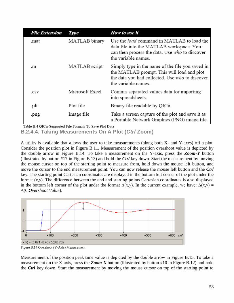
choose from are listed and described in Table B.4.
58
B.2.4.4. Taking Measurements On A Plot (Ctrl Zoom)
A utility is available that allows the user to take measurements (along both X- and Y-axes) off a plot.
Consider the position plot in Figure B.11. Measurement of the position overshoot value is depicted by
the double arrow in Figure B.14. To take a measurement on the Y-axis, press the Zoom-Y button
(illustrated by button #17 in Figure B.13) and hold the Ctrl key down. Start the measurement by moving
the mouse cursor on top of the starting point to measure from, hold down the mouse left button, and
move the cursor to the end measurement point. You can now release the mouse left button and the Ctrl
key. The starting point Cartesian coordinates are displayed in the bottom left corner of the plot under the
format (x,y). The difference between the end and starting points Cartesian coordinates is also displayed
in the bottom left corner of the plot under the format Δ(x,y). In the current example, we have: Δ(x,y) =
Δ(0,Overshoot Value).
Figure B.14 Overshoot (Y-Axis) Measurement
Measurement of the position peak time value is depicted by the double arrow in Figure B.15. To take a
measurement on the X-axis, press the Zoom-X button (illustrated by button #10 in Figure B.12) and hold
the Ctrl key down. Start the measurement by moving the mouse cursor on top of the starting point to

59
measure from, hold down the mouse left button, and move the cursor to the end measurement point. You
can now release the mouse left button and the Ctrl key. The starting point Cartesian coordinates are
displayed in the bottom left corner of the plot under the format (x,y). The difference between the end and
starting points Cartesian coordinates is also displayed in the bottom left corner of the plot under the
format Δ(x,y). In the current example, we have: Δ(x,y) = Δ(Peak Time Value,0).
Figure B.15 Peak Time (X-Axis) Measurement
Similarly, measurements along both X and Y axes can also be taken simultaneously by using the Zoom-
XY button (illustrated by button #9 in Figure B.12) and holding the Ctrl key down.
B.2.5. Signal Generator
Most QICii modules have a signal generation utility which can be used, for example, to generate the
DCMCT motor voltage in open-loop (like in the Modelling laboratory) or the reference signal to a
closed-loop system. If present, the signal generator input frame is located on the left-hand side of the
QICii module window, as shown in Figure B.11.
Furthermore, it is detailed in Figure B.16 where every input parameter defining the generated signal is
identified through the use of an ID number.
Figure B.16 QICii Signal Generator
Table B.5 provides a description of each input parameter defining the generated signal, as numbered in
Figure B.16.

60
The actual implementation of the QICii signal generator is described in the following subsections.
B.2.5.1. Square Wave
When button #3 in Figure B.16 is pressed, the QICii signal generator outputs a square wave as a
function of the Amplitude, Frequency, and Offset input parameters. This is illustrated in Figure B.17.
Figure B.17 QICii Square Wave Generation
Mathematically, the generated square wave signal, r(t), can be characterized by the following piecewise-
continuous function:

61
where t is the continuous time variable, Ampli the Amplitude input, Freq the Frequency input, Offset the
Offset input, and [ ] the modulo function.
B.2.5.2. Triangular Wave
When button #1 in Figure B.16 is pressed, the QICii signal generator outputs a triangular wave (a.k.a.
sawtooth signal or ramp) as a function of the Amplitude, Frequency, and Offset input parameters. This is
illustrated in Figure B.18.
Figure B.18 QICii Triangular Wave Generation
Mathematically, the generated triangular wave signal, r(t), can be characterized by the following
piecewise-continuous function:
62
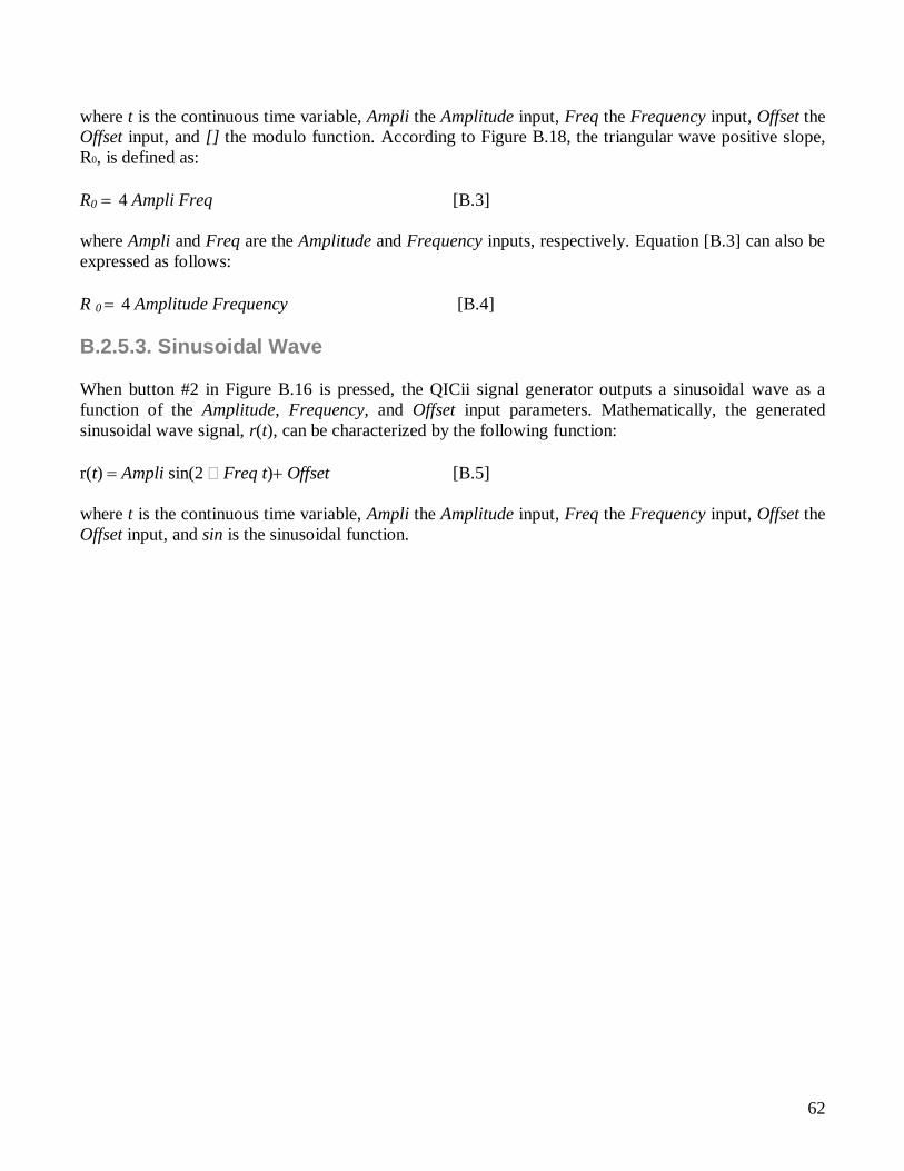
where t is the continuous time variable, Ampli the Amplitude input, Freq the Frequency input, Offset the
Offset input, and [] the modulo function. According to Figure B.18, the triangular wave positive slope,
R0, is defined as:
R0 4 Ampli Freq [B.3]
where Ampli and Freq are the Amplitude and Frequency inputs, respectively. Equation [B.3] can also be
expressed as follows:
R 0 4 Amplitude Frequency [B.4]
B.2.5.3. Sinusoidal Wave
When button #2 in Figure B.16 is pressed, the QICii signal generator outputs a sinusoidal wave as a
function of the Amplitude, Frequency, and Offset input parameters. Mathematically, the generated
sinusoidal wave signal, r(t), can be characterized by the following function:
r(t) Ampli sin(2 Freq t)Offset [B.5]
where t is the continuous time variable, Ampli the Amplitude input, Freq the Frequency input, Offset the
Offset input, and sin is the sinusoidal function.
63
LAB 4
System Modeling
Contents:
Introduction Nomenclature
Practice first principles modeling Reading Motor datasheets
Developing motor transfer functions in MATLAB using the CS toolbox
Determining System Parameters
Pre-lab results summary table
Modeling module graphical user interface Module Startup
Static Relations
Dynamic Models
In-lab results summary table

64
2.3. Introduction Modelling is an essential aspect of control. The key elements of modelling are:
Get an overview of the system and its components.
Understand the system and how the system works.
First principles component modelling.
Modelling from experimental tests – Parameter Estimation.
Disturbances.
Model Uncertainty.
Model Validation.
An overview of the system can be obtained by pictures, schematic diagrams, and block
diagrams. This gives representations of a system which emphasizes the aspects of the
system that are relevant for control and suppresses many details. The work is guided by
focusing on the variables that are of primary interest for control.
The block diagram gives a natural partition of the system. Mathematical descriptions of the
behaviour of the subsystems representing each block is necessary to have a complete
model. In control it is often sufficient to work with linearized models where dynamics are
represented by transfer functions. These transfer functions can be obtained from first
principles by applying the basic physical laws that describe the subsystems or by
experiments on a real system. First principles modelling requires a good knowledge of the
physical phenomena involved and a good sense for reasonable approximations.
Experiments on the actual physical system are a good complement to first principles
modelling. This can also be used when the knowledge required for first principles
modelling is not available. It is good practice to start the experiments by determining the
static input-output characteristics of the system. For systems with several inputs as the
motor in the DCMCT one can often obtain additional insight by exploiting all inputs.
Models can also be obtained by exciting the system with an input and observing the system
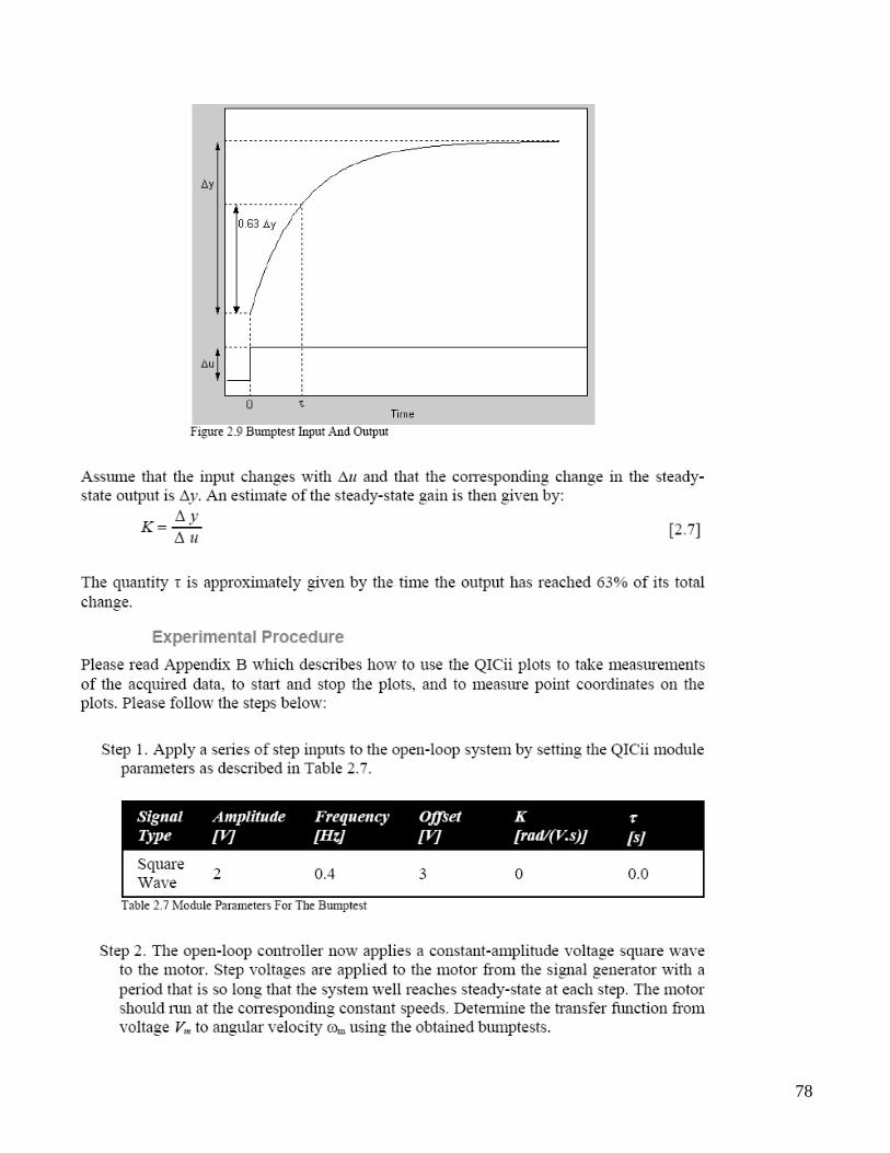
variables. The so called “bump-test” is a simple method based on a step response.
Frequency response is another useful technique where a sinusoidal input is applied and the
steady-state response is observed. Frequency response has the advantage that very accurate
measurements can be obtained by using correlation techniques. A model can in principle be
obtained by applying any type of input to the system and analyzing the corresponding
response. There is abundant literature and good software available to do this. In this lab we
will emphasize simple methods.
Even if linear models are often adequate for control it is important to have an assessment of
the major nonlinearities of a system. Saturation of actuators is one nonlinearity that is
important for all control systems.
Disturbances are often an important issue in control system design. They may appear both
as load disturbances which drive the system away from its desired behaviour and
measurement noise that distorts the information about the system obtained from the sensors.

65
An assessment of the disturbances is an important part of modelling for control.
When determining parameters experimentally it is customary to also provide estimates of
the accuracy of the parameters. Similarly when modelling dynamical systems for the
purpose of controlling them, it is also essential to provide some measure of model accuracy.
When modelling dynamical systems the precision of a model can be expressed in terms of
the accuracy of the parameters. This is however not sufficient because there may be errors
due to neglected dynamics. It is important for design of control systems to make some
assessment of this unmodeled dynamics. An assessment of the unmodeled dynamics is
therefore an important aspect of modelling for control.
When a model is obtained, it is good practice to assess the validity of the model by running
simulations of the model and comparing its response with that of the actual system. Model
validation is an important step that should be performed in order to give a level of
confidence in the expected performance of the closed-loop system.
2.4. Nomenclature The following nomenclature, as described in Table 2.1, is used for the system open-loop
modelling.

66
2.5. Pre-Laboratory Assignments: First Principles Modelling The DCMCT motor, inertial load, power amplifier, encoder, and the filter to obtain the
velocity are modelled by the Motor And Inertial Load subsystem, as represented in Figure
2.1. The block has one input the voltage to the motor Vm and one output the angular
velocity of the motor ωm. Additionally, a second input is also considered: the disturbance
torque, Td, applied to the inertial load.

67
Figure 2.1 The Motor And Inertial Load Subsystem
In the following, the mathematical model for the Motor And Inertial Load subsystem is
derived through first principles.
2.5.1. Motor First Principles Please answer the following questions.
1. When using SI units, the motor torque constant, kt, is numerically equal to the back-electro-
motive-force constant, km. In other words, we have:
k t km [2.1]
This workbook uses the SI (International System) units throughout and the motor
parameter named km represents both the torque constant and the back-electro-motiveforce
constant.
Considering a single current-carrying conductor moving in a magnetic field, derive an
expression for the torque generated by the motor as a function of current and an
expression for the back-electro-motive-force voltage produced as a function of the shaft
speed. Show that both expressions are affected by the same constant, as implied in
relation [2.1].
2. Figure 2.2 represents the classic schematic of the armature circuit of a standard DC
motor.

68
Figure 2.2 DC Motor Electric Circuit
Determine the electrical relationship characterizing a standard DC motor.
3. Determine and evaluate the motor electrical time constant τe. This is done by assuming
that the shaft is stationary. You can find the parameters of the motor in Table A.2.
4. Assume τe is negligible and simplify the motor electrical relationship previously determined.
What is the simplified electrical equation?
5. Neglecting the friction in the system, derive from first dynamic principles the mechanical
equation of motion of a DC motor. Determine the total (or equivalent) moment of inertia
of motor rotor and the load.
6. Calculate the moment of inertia of the inertial load which is made of aluminum. Also,
evaluate the motor total moment of inertia. The motor data sheet is given in Table A.2.

69
2.5.2. Static Relations Modelling by experimental tests on the process is a complement to first principles
modelling. In this section we will illustrate this by static modelling. Determining the static
relations between system variables is very useful even if it is often neglected in control
systems studies. It is useful to start with a simple exploration of the system.
Please answer the following questions.
1. Assuming no disturbance and zero friction, determine the motor maximum velocity:
ωmax.
2. Determine the motor maximum current, Imax, and maximum generated torque, Tmax.
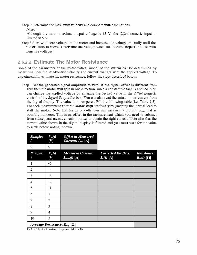
3. During the in-laboratory session you will be experimentally estimating the motor
resistance Rm. This can be done by applying constant voltages to the motor and
measuring the corresponding current while holding the motor shaft stationary.
Derive an expression that will allow you to solve for Rm under these conditions.
4. During the in-laboratory session you will be experimentally estimating the motor torque
constant km. This can be done by applying constant voltages to the motor and measuring
both corresponding steady-state current and speed (in radians per second).
Assuming that the motor resistance is known, derive an expression that will allow you to
solve for km.
What is the effect of the inertia of the inertial load on the determination of the motor
constant?
5. Applying first principles, find an estimate of the measurement noise, eω, present in the
velocity signal ωm. Note that the encoder resolution is 4096 counts per revolution and the
sampling period h is 0.01 s.
Hints:
Consider the position measurement error eθ.
You can also use eh the error in the sampling interval (a.k.a. jitter).
The following series expansion can also be relevant:
[2.2]
2.5.3. Dynamic Models: Open-Loop Transfer Functions Please answer the following questions.
1. Determine the transfer function, Gω,V(s), of the motor from voltage applied to the motor
to motor speed.
Hint:
The motor armature inductance Lm should be neglected.
2. Express Gω,V(s) as a function of the parameters a and b, defined such as:
[2.3]
3. Express Gω,V(s) as a function of the parameters K and τ, defined such as:
[2.4]
4. Determine the transfer function, Gω,T(s), from disturbance torque applied to the inertial
load to motor speed. Express Gω,T(s) as a function of the parameters KTd and τTd, as

70
defined below:
[2.5]
Show that
5. From your previous calculations and the motor parameters given in Table A.2,
summarize the system parameter values relevant to evaluate the tranfer functions derived
so far.
6. Evaluate both transfer functions Gω,V(s) and Gω,T(s), as well as their parameters a, b, K, τ,
and KTd.
7. Derive using basic blocks (gain, integrator, summer) the plant open-loop block diagram.
8. Simplify the obtained open-loop block diagram so that it has the block structure depicted
in Figure 2.4. Fill up the empty blocks.
Figure 2.4 Simplified Open-Loop Block Diagram Template
9. The transfer function Gω,V(s) previously derived is only an approximation since the
inductance of the motor has been neglected. Considering the motor electrical time
constant τe previously evaluated, justify the approximation.
2.5.4. Pre-Laboratory Results Summary Table Table 2.2 should be completed before you come to the in-laboratory session to perform the
experiment.

71

72

73

74
75

76

77
78

79

80

81

82
83
LAB 5
Speed Control
Contents:
Introduction to the PI controller PI control law (set-point,Kp,Ki)
Magic of Integral action Nomenclature Pre-labassignment PI controller design to given specifications using MATLAB CS toolbox.
Tracking triangular signals (power of time input)
Response to load disturbances
Pre-labresults summary table
Speed control module graphical user interface Module Description/Startup
Qualitative properties of proportional and integral control
Manual Tuning using ZieglerNichols
Design to given specifications
Tracking triangular signals (power of time input)
Response to load disturbances
In-lab results summary table

84

85

86

87

88

89

90
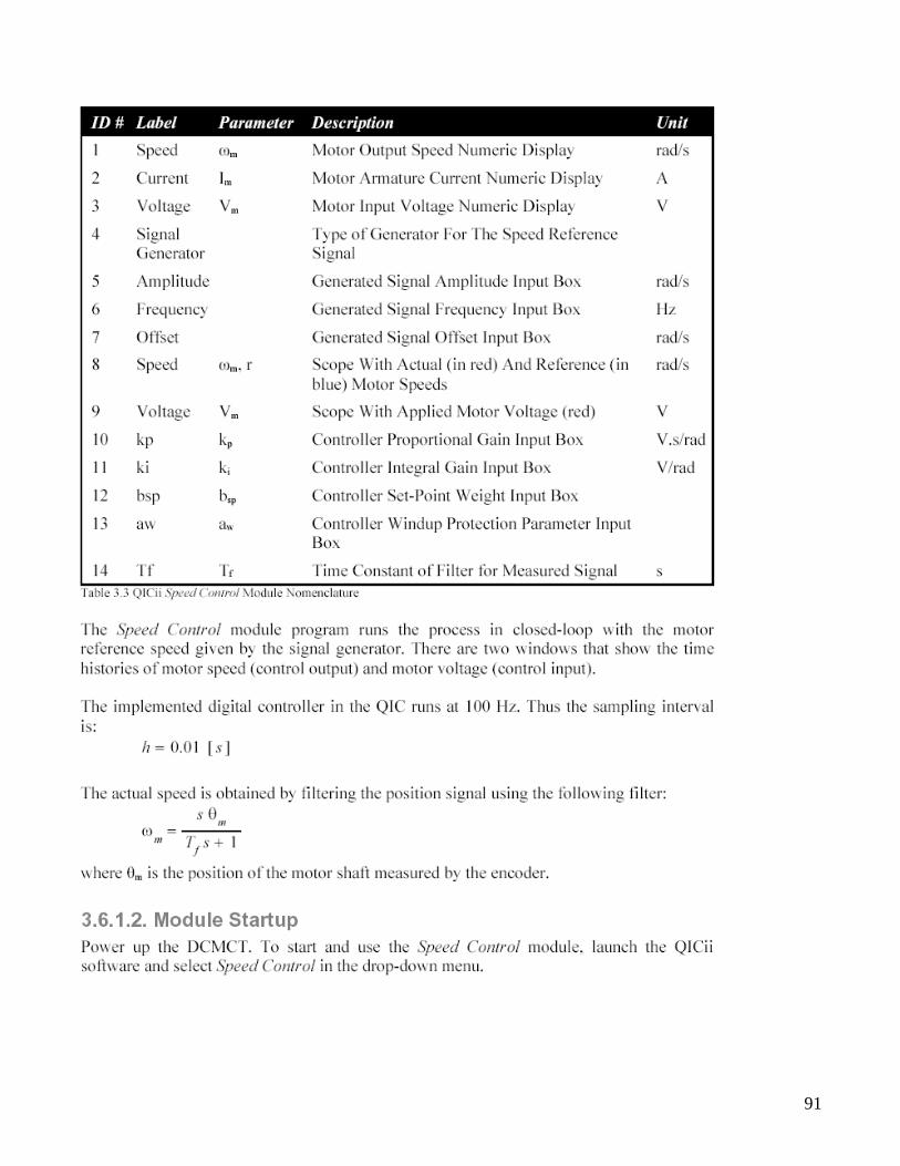
91

92

93

94

95

96

97

98

99
LAB 6
Position Control
Contents:
Introduction to the PID controller PI control law (set-point,Kp,Ki)
Magic of Integral action
Controller with two degrees of freedom Nomenclature Pre-labassignment Comparison between PD position and PI speed control
Fundamental limitations and achievable performance
PD controller design to given specifications using MATLAB CS toolbox.
Tracking triangular signals (power of time input)
Response to load disturbances
Pre-labresults summary table
Position control module graphical user interface Module Description/Startup
Qualitative properties of proportional and derivative control
Design to given specifications
Tracking triangular signals (power of time input)
Response to load disturbances
In-lab results summary table
100

101

102

103

104

105

106

107

108

109

110

111

112

113

114

115

116

117

118
119

120
LAB 7
Robust Control
Contents:
Introduction Nomenclature
Pre-labassignment MATLAB script
Robustness and Sensitivity
Stability Margins
Pre-labresults summary table
Robustness module graphical user interface Module Description/Startup
stability margin evaluation
In-lab results summary table

121

122

123

124

125

126

127

128

129

130

131

132

133

134
135

136

137

138

139

140

141