AUGUST 1984 UDS-TH- 1396

CaResearch Supported By:

U Defense Advanced ResearchProjects Agency-ContractNOOO1484-K-0357 S S

National Science FoundationContract NSFECS-8310698

* -

THE DESIGN AND PERFORMANCE ANALYSIS

OF AN ARBITER FOR A MULTI-PROCESSOR

SHARED-MEMORY SYSTEM S

Shahrukh S. Merchant

198

LA.0

Laboratory for Information and Decision Systems

MASSACHUSETTS INSTITUTE OF TECHNOLOGY, CAMBRIDGE, MASSACHUSETTS 02139

This document has been approved

for public release and sale; its

distribution is unlimited.

84 09 2 1 057

August 1984 LIDS-TH--1396

THE DESIGN AND PERFORMANCE ANALYSIS OF AN ARBITER

FOR A MOLTI-PROCESSOR SHARED-MEMORY SYSTEM

by

Shahrukh S. Merchant

This report is based on the unaltered thesis of Shahrukh S. Merchantsubmitted in partial fulfillment of the requirements for the degreeof Master of Science at the Massachusetts Institute of Technology inSeptember 1984. This research was conducted at the M.I.T. Laboratoryfor Information and Decision Systems with partial support provided bythe Defense Advanced Research Projects Agency under Contract N00014-84- 0K-0357 and by the National Science Foundation under Contract NSF-ECS-8310698.

Laboratory for Information and Decision SystemsMassachusetts Institute of Technology

Cambridge, Massachusetts 02139

........

. . - ... o. .

Encl (1)

SECURVY CLASSIFICATION OF ?111% PAGE9 (35..M 000 Dmiff. UNCLASSIFIEDRZD WTRUCTIONS

.20 UNREPORT DOCUMENTATION PAGE 29EvR COMPtEMw FORM3. GOPOT ACCESSIO L. 11CIMGM CATALOG NUNOeR~

4. TITLE (and &a451e3 a. TYPE or REPORT a PEROD COV61REC

THE DESIGN AND PERFORMANCE ANALYSIS OF AN ThesisARBITER FOR A MJLTI-PROCESSOR SHARED-MEMORY _____________

SYSTEM4 6. PERFORMING altG. REPORT NUMBER____ ___ ___ ___ ____ ___ ___ ___ ____ ___ ___ ___LIDS-in- 1396

*7. A4JTNORfa) 11. CONTRACT OR GRANT NUNUER(.e)DARPA Order No. 3045/2-2-84

Shahrukh S. Merchant Amendment #11ONR/N0014-84-K-03S7

S. PRFORINGGROAIZAION AME ND DDRES 4. PROGRAM CLEMENT. PROJECT. TASKS. ERFRMNG RGAIZTIO NAE NO OONESAREA & ORK UNIT NUM1RS11

Massachusetts Institute of Technology Program Code No. ST10Laboratory for Information and Decision Systems ONR Identifying No. 049-383Cambridge, Massachusetts 021-39 ______________

*It. CONTROLLING OFFICE MNM ARC A000RE314 12. REPORT DATEDefense Advanced Research Projects Agency August 19841400 Wilson Boulevard IS. MUMMUR OF PAGES

Arlington, Virginia 22209 10414. MONITORING AGENCV NAME A AORSS(1dift.er bea Cw.1litg 0111.) 15. SECURITY CLASS. (W1 de~i ftpeeOffice of Naval Research UNCLASSIFIEDInformation Systems ProgramCode 437 11& SIFICATIO3 *^ANGRAING

Arlington, Virginia 22217 _____________

I&. GISTRISUTIWON STATEMIENT Fat -. e RAse

Approved for public release: distribution unlimited

I7. DISTRIBUTION STATEMEN4T (&I the a680'ft 60ee Ift 1110" 26. it 10et *ew A GPetl

*IL. SUPPLEMENTARY NOTES

19I. Kay WONOS; (C"N. a #we e Shia M use.a aid I*.N'i by blooN urnS..)

26. ABSTRACT (CUU..m an v,wa. side It Us*ovew oE ~Jrur We* Slobe..

A "round-robin" arbiter has been designed and implemented for sharing memoryin a multi-processor system. A study is made, via analysis and simulation, ofthe performance of this arbiter under various load conditions. In particular,distributions are obtained for the-waiting time of an arriving customer undervarious load conditions, and expressions are obtained for the idle timedistribution and the mean busy time.

D0 I, ON 1475 30171G OF 1 Nov as is oUSolETES/N 0 102. L- 61 A. 4601 SE 0IT 6IASSIFICATIOR 0#1 THIS past (Wh32 &%we*

. . . ..

UNCLASSIFIED

20. Th effet of: heavy or light user in the midst of other moderate users-is also examined, as isthe effect of longer guaranteed idle periods by individual-customers after a service completion.

M~ny of the results obtained with a rounmd-robin arbiter are compared with thoseobtained using at First-come, First-served arbiter. In the course of doing this,a simple relation has been found between the waiting time distribution and the

* distribution of the number of customers in any discrete-time First-come, First-served system with a single work-conserving deterministic server.

Accession For - .- -

* ~NTIS C~

1" M -0-L6a -44

UCtURI1Y CIASOFICAT4OF vT1413 PAOafuim DOMata hem

The Design and Performance Analysis

of an Arbiter

for a Mult i-Processor Shared-Hemory System

by

Shahrukh S. Merchant

B.S., University of Wisconsin, Madison, 1981

Submitted to the Department ofElectrical Engineering and Computer Sciencein partial fulfillment of the requirements of

the Degree of-

Master of Science in 2lectrical Engineering and Computer Science

at the

Massachusetts Institute of Technology

September 1984

* Massachusetts Institute of Technology, 1984

Signature of Author .. )(vepartment of Electrical Engineering and

Computer Science, 24 July, 1984

Certified by________________________Prof. R.G. Gallager, Thesis Supervisor

Accepted by _________________________Chairman, Electrical Engr. and Computer Scince

2

TABLE OF CONTENTS

TABLE OF CONTENTS 2

LIST OF FIGURES AND TABLES 5

ABSTRACT 6

ACKNOWLEDGEMENTS 7

PART I: DESIGN AND IMPLEMENTATION

1. INTRODUCTION TO CLUMPS 9

1.1. Purpose and Philosophy of CLUMPS 9

1.2. Outline of CLUMPS architecture 111.2.1. Architecture of a node1.2.2. Overall architecture1.2.3. Software

1.3. Functions of global memory unit 13

2. ROLE OF ARBITER IN GLOBAL MEMORY UNIT 15

2.1. Function of arbiter 15

2.2. Functional specifications of arbiter 152.2.1. Interface between global memory board and

branches2.2.2. Performance considerations

2.3. The around-robin" solution 172.3.1. Comments on fairness2.3.2. Rejection of a First-come, First-served

(FCFS) arbiter

PART II: PERFORMANCE ANALYSIS AND SIMULATIONS

3. THE BASIC SYMO4ETRIC MODEL 24

3.1. Setting up a simplified model 243.1.1. Nomenclature3.1.2. Modelling the system exactly3.1.3. Modelling as a First-come, First-served

(FCFS) system3.1.4. Results to be sought

3.2. Distribution of the number of customers 28

. . ............... . .. . . .. ,... ., .... .. . .. ... -.. .,- .

3

3.3. Distribution of waiting times in FCFS model 323.3.1. Derivation based on "counting" arguments3.3.2. An alternative derivation

3.4. Simulation results: waiting time in round-robin model 37

3.5. Idle and busy periods 393.5.1. Distribution of idle periods3.5.2. Mean length of a busy period

3.6. Fairness characteristics of the biased arbiter 413.6.1. Simulation results3.6.2. Relation to frequency of idle periods

4. EFFECT OF A SINGLE HEAVY OR LIGHT USER ON FAIRNESS 45.......

4.1. Round-robin arbiter 45

4.2. First-come, First-served (FCFS) arbiter 48

4.3. Round-robin vs. FCFS 50

5. EFFECT OF LONGER GUARANTEED IDLE TIME AFTER REQUESTS 52

5.1. Relaxations of restrictions on present model 52

5.2. Decreasing randomness 53

6. CONCLUSIONS AND SUMMARY 56

REFERENCES 58

APPEND KCR8

A. HARDWARE DESCRIPTION 60

A.1. CLUMPS global bus specifications 60A.1.1. Bus signalsA.1.2. Global memory map

A.2. Global memory board design 63A.2.1. Schematic diagramA.2.2. Parts list

A.3. Global memory board operation 69A.3.1. Overview of circuit operationA.3.2. Timing diagrams

A.4. PAL implementation of logic 72A.4.1. Bus address decoderA.4.2. Miscellaneous logic

............

4

A.5. PAL implementation of arbiter 76A.5.1. Fair arbiterA.5.2. original arbiter design

B. ANALYSIS AND SIMULATION SOFTWARE 83

3.1. Listing of program to calculate parameters forFCFS model 83

3.2. Simulator listing 90

5

LIST OF FIGURES AND TABLES

Figures

1.1. A configuration of CLUMPS nodes1.2. Structure of a CLUMPS node3.1. Markov chain for FCFS model3.2. Distribution of number of customers in the system, for

various p.3.3. One-to-one correspondence between waiting times of

arrivals and number of customers in system3.4. Waiting time distributions for round-robin and FCFS

models3.5. Mean waiting time for all devices (p-0.07)5.1. Mean waiting time as a function of number of guaranteed

idle cycles, for various values of "mean time torequest."

A.I. Implementation of a CLUMPS nodeA.2. CLUMPS Global Memory schematic diagramA.3. Timing waveforms for global memory boardA.4. Globa memory decoder PALA.5. Schematic diagram for "random" logic implemented on U3A.6. Schematic diagram for "random" logic implemented on U10 :A.7. Schematic diagram for arbiter PAL

Tables

3.1. Smallest and largest mean waiting times for devices, atvarious request probabilities

4.1. Waiting times for device 0 and other devices as afunction of request probabilities of device 0 and otherdevices (round-robin arbiter)

4.2. Waiting times for device 0 and other devices as afunction of request probabilities of device 0 and otherdevices (FCFS arbiter)

A.1. CLUMPS Global bus pinoutsA.2. CLUMPS Global memory boardA.3. CLUMPS Global memory board parts listA.4. Global memory waveform generation

id. I

I--

~. .. . .o

,. , .

/ 60

ABSTRACT

)A und-robint' arbiter has been designed and

implemented for sharing memory in a multi-processor system.

A study is made, via analysis and simulation, of the

performance of this arbiter under various load conditions.

In particular, distributions are obtained for the waiting

time of an arriving customer under various load conditions,

and expressions are obtained for the idle time distribution

and the mean busy time.

The effect of a heavy or light user in the midst of

other moderate users is also examined, as is the effect of

longer guaranteed idle periods by individual customers after

a service completion.

Many of the results obtained with a round-robin arbiter

are compared with those obtained using a First-come,

First-served arbiter. In the course of doing this, a simple

relation has been found between the waiting time

distribution and the distribution of the number of customers

in any discrete-time First-come, First-served system with a

single work-conserving deterministic server.

_m-

0 ?:?::

7

ACXNOVLZDGZNEMTS

This work was supported in part by grants from the

National Science Foundation (NSF-ECS-8310698) and the

Defense Advanced Research Projects Agency (N00014-84-

K-0357).

I would like to extend my appreciation to my thesis

advisor and graduate counsellor, Prof. Robert Gallager for

his constant interest and supportive attitude, and to

Mr. Daniel Helman for his many helpful ideas and for the

fruitful discussions I have had with him.

0".

C • °

"3 °- "

3i:'-'

7r7

PART I

DESIGN AND IXPLEENMAT ION

9

1. INTRODUCTION TO CLUMPS

The focus of this thesis is the design and analysis of

the arbiter used in the Communications LangUage

Multi-Processor System (CLUMPS). The purpose of this

section is to acquaint the reader with the basic structure

of (CLUMPS), so as to provide some perspective for the role

of the arbiter in the system. This section is, therefore,

global and brief in its description of the CLUMPS system;

the reader is referred to (HEL84] for details.

1.1. Purpose and Philosophy of CLUMPS

The Communications LangUage Multi-Processor System

(CLUMPS) is a project at the Laboratory for Information and

Decision Systems (LIDS) for building a -truly distributed

Computer Communications Network [GAL83, HEL82, HEL84,

TUB83]. A typical network is shown schematically in Figure

1.1..-

The system consists of several nodes, connected

together in an arbitrary topology via branches. The system

is truly distributed in the sense that all its nodes are

heirarchically equal; there is no master-slave

relationship. (l)

(1) The *host" connected to a node in Figure 1.1 exists onlyfor the purpose of initializing the system andcollecting performance data. Its existence does notimply that the node to which it is connected has a

....... 7

10

SBranches.

Figure 1.1. A configuration of CLUMPS nodes.

The network is to be used in the real-time simulation

of network control algorithms such as those that control

flow and congestion in networks, including, but not

restricted to, communication networks. The idea is that one

can effect faster, more realistic simulations on a real

network than by simulating the network entirely via software

on a computer. Additional details on the philosophy of

CLUMPS may be found in (H3L84].

privileged status.

S. . .-. .-.

.- .-.

11 -

1.2. Outline of CLUMPS architecture -

1.2.1. Architecture of a node

Each node shown in Figure 1.1 contains processing,

storage and communications capabilities. As shown in Figure

1.2, each node can have up to eight branches, with which it

Processors

Figure 1.2. Structure of a CLUMPS node

may be connected to other nodes. The processing power of a

node is contained in eight microprocessors, one associated

with each branch. The processors communicate with each

other only through a region of global memory, shared by all

the processors in a node. These processors are closely

coupled, in that computational tasks required of a node are

allocated to idle processors by the operating system in a

way that is transparent to any process outside the node.

For all practical purposes, therefore, one may think of the

processing power of a node as residing in a single .

• °° - .. . . ,.. .. . . . i ' "'"" " " " '

12

processing unit. Note, however, that there is no central

processor that has a distinct master role in controlling the

other processors within a node. The CLUMPS system is thus

distributed in two independent (and unrelated) ways:

firstly, processing is distributed at the network level (all

nodes are "equal") and, secondly, at the node level (all

processors within a node are "equal").

See Appendix A, [HEL83] and [MER82] for additional

details on the CLUMPS architecture.

1.2.2. Overall architecture

Each branch in a node is implemented as a serial

communication line. A 64 x 64 electronic crossbar switch

[LEB84] permits the configuration of arbitrary topologies

with up to 64 branches.

The host, shown in Figure 1.1, is an IBM Personal

Computer, responsible for loading the operating system

software into all the nodes in the network upon power-up or

system reset. It may be programmed to receive performance

and statistical data on the algorithms being simulated on

the network.

1.2.3. Software

The primary language supported by the system is the

high-level language NIL (Network Interface Language) [PAR82,

BUR82, NIK84], developed at the IBM Research Center in

Yorktown Heights, New York. This language was chosen

. -. • .

13

because of its suitability for distributed multiprocessor

systems for communications applications.

The NIL compiler [HEL84, NIK84] does not generate

native machine code for the branch processors (which are

Motorola 6809 processors [MOTd1]); it generates an

intermediate sequence of "pseudo-opcodes" which are

interpreted at run-time by an interpreter that is resident

at each processor. Although this 2-stage approach results

in slower execution, it was chosen because it results in

very compact code and facilitates sharing of processes.

This, in turn, leads to fewer global memory cycles which

could otherwise be a potential bottleneck. It is also

easier to implement and test and results in a more

transportable compiler.

A distributed operating system runs at each node to

allocate or queue tasks to any of the eight processors in a

way that is transparent to the application program. See

[HEL84] for details on the functioning of the operating

system.

1.3. Functions of the global memorv unit

The "global memory unit" could, more accurately, be

called a "global functions unit" for, in addition to (a)

read/write memory, it also contains b) a programmable -

counter/timer, lc) circuitry to allow any of the

microprocessors in a node to identify the node as well as

the branch (within the node) with which it is associated and

- . . . .* *. . . . . .- ,.. . . . . . .

14

(di logic to allow any branch to reset the node or to

generate an interrupt to all processors within a node.

The read/write memory is, however, the primary function

of the global memory unit. It is used by the processors

comprising a branch in two ways: 1) to store the

intermediate compiled NIL code for interpretation by the

interpreter and 2) to store data packets en route to or from

other nodes.

Appendix A contains a complete schematic diagram for

the entire global memory unit, including a memory map,

timing diagrams and a description of circuit operation. L

! L

15 ...

2. ROLE OF ARDITIR IN GLOBAL )MXORY UNIT

2.1. Function of arbiter,

As stated earlier, the global memory unit is shared by

up to eight processors, only one of which has access to it

at any given time. The function of the arbiter is to (a)

accept requests for access to the global memory from the

processors, b} decide which one gets access for the next

cycle in the event that two or more processors have requests

pending and (a) signal its decision to the processor chosen.

2.2. Functional specifications of arbiter

2.2.1. Interface between global memory board and branches

In addition to the common bus signals shared by the

global memory and branch boards, each branch has a pair of

request-acknowledge lines connecting it to the arbiter on

the global memory board. A branch processor makes a request

by asserting its active-low request line to the logic 0

state. The request line stays in this state until the

arbiter grants the request by asserting the corresponding

acknowledge line (driving it to logic 0). Upon receiving

the acknowledge signal, the requesting device removes its

request and proceeds to use the following memory cycle for a

read or write. The acknowledge stays active (low) for the

duration of the cycle (a constant 400 nu at the clock rate

used).

For convenience in identifying devices (branch

.......................... . . . "

.... , . .• I

16

processors), we will number them from 0 to 7, and refer to

their request and acknowledge signals as Req i and Acki

respectively, for i in the range of 0 to 7.

2.2.2. Performance considerations

An important requirement of the arbiter is that it be

fair; all eight devices should receive equal priority

service, on the average. The reason for this is that all

branches of a node should perform identically; the hardware

should not introduce a bias caused by asymmetric performance

of the branches.

Furthermore, due to restrictions on how long memory

cycles of a processor can be "stretched" (MOT81], the

waiting time of a device must be bounded. A straightforward

way to achieve this is to require that while any branch has

a request pending, no other branch can have more than one

request serviced. This guarantees that the waiting time for

any device is at most eight cycles.

As a request must be latched and stable well before the

start of a memory cycle which is affected by that request,

sufficient "pipelining" of requests (about half a cycle)

should be provided so that there is no "dead time" between

memory cycles to process requests. For reasons of

L °i

-L .

, - o. ,

17

efficiency, we will also require that the arbiter not be

idle as long as there are requests pending.(1)

2.3. The "round-robin" solution

The above requirements can be met by a so-called

round-robin arbiter. This arbiter serves device #0, device

#1 and so on, up to device #7, and then returns to serving

device #0. Of course, those devices not making requests are

skipped.

Another way of describing this strategy is as follows:

If device i was the, last one served, then; for the next

cycle, device (i+1) mod 8 has the highest priority, device

(i+2) mod 8 the next highest priority, and so on, with

device (18) mod 8 (which is just device i) having the

lowest priority.

The equation describing the next-cycle status of each

of the 8 acknowledgement signals, Acki', as a function of

current requests, Reqi, and current acknowledgement signals,

Acki is:

(1) An exception to this is when cycles are "stolen'occasionally for refreshing the dynamic memory. SectionA.3 has details.

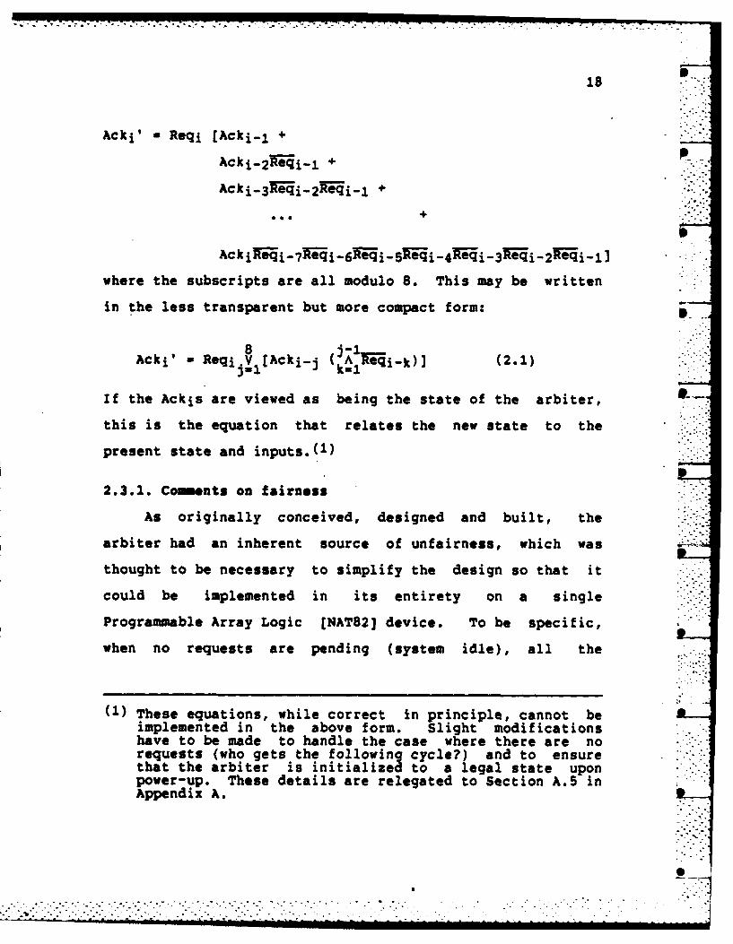
Ack i ' = Reqi [Acki-1 +

Acki_2- i_1 + p) ;i

where the subscripts are all modulo 8. This may be written

in the less transparent but more compact form:

8 j-1Acki' = Reqi V[Acki-j li- k)( (2.1)

If the Ackis are viewed as being the state of the arbiter, -

this is the equation that relates the new state to the

present state and inputs.(1 )

2.3.2. Coments on fairness

As originally conceived, designed and built, the

arbiter had an inherent source of unfairness, which was

thought to be necessary to simplify the design so that it

could be implemented in its entirety on a single

Programmable Array Logic CNAT82] device. To be specific,

when no requests are pending (system idle), all the

(1) These equations, while correct in principle, cannot beimplemented in the above form. Slight modificationshave to be made to handle the case where there are norequests (who gets the following cycle?) and to ensurethat the arbiter is initialized to a legal state uponpower-up. These details are relegated to Section A.5 inAppendix A.

o..

19

acknowledgement lines, which also serve to retain the

arbiter state, are inactive. Thus, should two or more

devices simultaneously make a request in a subsequent cycle,

one cannot tell which one should get served first based on

the number of the last served device, because this

information has not been retained. The solution, in the

original version of the arbiter, was to simply give

lower-numbered devices priority in this case, and was chosen

because it was easily implemented.

It was believed that this would have a negligible

effect on fairness because it only happens when (a) the

system is idle and (b) two or more devices make requests

simultaneously. If (a) occurs with high probability thenthe system is very lightly loaded and (b) will occur with

low probability. The hypothesis that this would not have a

significant effect on fairness was tested via simulation.

The results, shown in Section 3.6, reveal that in the case

of all devices having equal frequency of requests, there

could be significant unfairness between the most favoured

device (#0) and the least favoured device (#7), as measured

by the difference between the mean waiting times for these

devices. At very low and very high loading, the difference

was a few percentage points and could be considered small.

However, for the intermediate values of loading most likely

to be encountered in the system, the difference in mean

waiting times between devices 0 and 7 was higher than 20% in

20

some cases,

This was deemed unacceptable as it could seriously skew

the results of algorithm simulations run on CLUMPS, so it

was decided to modify the arbiter design to make it truly

fair. Details are in Section A.5; basically the

modification consists of changing the state description of

the arbiter so that it reflects the last device served

(however long before) rather than just the device served, if

any, in the previous cycle. The increase in complexity of

the design was, fortunately, much smaller than originally

believed.

In the remainder of this document, the original arbiter

design shall be referred to as the biased arbiter and the

modified design the fair arbiter, if it is necessary to

distinguish between the two and the distinction is not clear

from context.

2.3.2. Rejection of a First-come First-served (FCFS) arbiter

As shown in Section 3.4, an arbiter which processes

requests in a first-come first-served manner has a more

regular behaviour than a round-robin arbiter in that the

waiting time distribution of the former has a smaller

variance than that of a round-robin arbiter (although they

both have the same mean waiting time). In the case where

all devices are generating requests with approximately equal

frequency, it seems an intuitively reasonable method to use.

The major reason for rejecting a FCFS arbiter is that _

• -:!.

21

it is considerably more complicated to implement. It

requires more memory than the round-robin arbiter as it

needs to maintain ranks for all devices with active

requests. This could, in the worst case, require the

arbiter to retain ordering information for eight previous

cycles.

This additional complexity is reflected in the number

of states required to implement the arbiter. For the

round-robin arbiter, we require only 8 states to retain the

identity of the last served device. For the FCFS arbiter,

we would require 81 = 40320 states (the number of ways that

the eight devices can be ranked) to retain the current ranks

of all 8 devices. A FCFS arbiter could not have been

implemented on a single programmable chip as was the

round-robin arbiter.

The resolution of simultaneous arrivals is also a more

difficult problem in a FCFS arbiter. For the round-robin

arbiter, this problem arose only when the system was idle,

and was fairly easy to solve, as described in Sections 2.3.1

and A.5.

9..

22

In the FCFS arbiter, one would, in effect, need a secondary

round-robin (or similar) scheme to resolve simultaneous

arrivals.(1)

p

()Another common problem with FCFS systems in general isthat a single very heavy user can monopolize theresources of the system; round-robin type solutions areusually superior in this respect. However, since adevice in our system cannot generate a request untilafter its previous request has been serviced, this isnot as severe a problem here. Results of simulationspresented in Section 4 show that if mean waiting time isused as a measure of fairness, a round-robin arbiter ismore "fair" than a FCFS one. For the FCFS arbiter, aheavy user could get as much as a 25% advantage inwaiting time over the other users. While hardlyastronomical, this difference could be significant insome applications.

preentd i Setio 4 howtha fmea watin tie i1l_

23

PART I I

PERFORMhNCE ANALYSIS AND SIMULATIONS

24

3. THE BASIC SYMMETRIC MODEL

3.1. Setting up a simplified model

To obtain useful results, it is desirable to model this

system as a Markov process; since the process is a

discrete-time one, we will model it as a discrete-time,

discrete-state Markov chain. To preserve the Markov

property without introducing a plethora of states, we assume

that for every cycle or time slot in which a device is not

active, there is a constant probability that it will

generate a request, independent of past history and of other

devices. The one exception is that a device cannot make a

request in the cycle immediately following one in which it

had access to the memory. This concession to reality can

fortunately be made without complicating the model unduly;

it is realistic because in practice the requests are

"pipelined" by about half a cycle, and since a device cannot

generate a request until after it has completed the current p.

memory cycle, it cannot generate another request in time to

get the following cycle. Furthermore, to simplify the

analysis, we assume that this constant probability of

generating a request, which we shall call 2,is the same for

all devices. All of Section 3 assumes that we are using the

fair arbiter (cf. Section 2.3.1).

3.1.1. Nomeuclature

In the terminology of queueing theory, requests by the

25

devices (processors) will be referred to as customer

arrivals. The granting of access to memory by the arbiter

and the subsequent completion of that memory cycle will be

referred to as a service cornpletion. Note that we have a

single server system that is work conserving (since the

server is always busy when there is work to be done). The

service is deterministic, i.e., it takes a constant time of.-

one unit. The arrivals are not memoryless since they depend

on the state of the system.

Similar nomenclature will be used in the rest of this

thesis.

3.1.2. Modelling the system exactly

Modelling the system completely requires a total of

about 211 or 2048 states (28 a256 states representing the

status--active or inactive--of the 8 input lines, times 8

for each of the 8 devices which may currently have

priority). Even allowing for the fact that all of these

states are not valid, there are far too many states to

obtain any useful analytic results. While there is some

symmetry in the system, it does not seem to permit ..

substantial simplification.

Therefore, it was decided to simulate the system to

obtain statistics on

a) the steady-state distribution, E, of the number of

customers and

b) the steady-state distribution, £.of the waiting

26

time of customers.

This simulation was performed on an IBM Personal Computer.

The simulation results are given in Section 3.4 and a Pascal

listing of the program appears in Appendix B.2. For

reference, the modelling of the complete system will be

referred to as the round-robin model.

3.1.3. Modelling as a First-come, First-served (FCFS) system

The round-robin discipline of the arbiter is not

first-come, first-served, but there are advantages to

modelling the system as such. Specifically, the identities

of the customers in the system are no longer important; for

the purpose of computing the distribution of the number of

customers and waiting times, it is sufficient to keep track

of only the number of customers (0-8) in the system. Thus, R

a 9-state Markov process is sufficient to model the system,

and the problem is analytically tractable. For reference,

this model will be referred to as the FCFS model.

In spite of the tremendous simplification resulting

from the FCFS assumption, one can still get useful results.

Specifically, since the server is work-conserving and all

customers are identical, it must be true that

a) the steady-state distribution of the number of

customers in the FCFS and round-robin models are

equal, since the number of customers in the system

and the arrival rates do not depend upon the

service discipline, and

27

b) the mean waiting time in the two models are the

same. Furthermore, one would expect, intuitively,

that the variance of the waiting time in the

round-robin model would be larger than that in the

FCFS model, since the latter is, in a sense, more

"regular."

3.1.4. Results to be sought .2

In Section 3, we will determine the distributions of

the number of customers in the system (Section 3.2) and

waiting time (Section 3.3) for the FCFS model and compare

these to those obtained via simulation for the actual

round-robin model (Section 3.4). Expressions will also be

derived for the distribution of idle periods in the system

and the mean length of a busy period (Section 3.5).

Finally, we will compare the fairness characteristics of the

"biased" and "fair" arbiters (Section 3.6).

The only variable parameter will be p, the probability A

of an inactive customer making a request.

JLA'""-

...................... . .:-

28

3.2. Distribution of the number of customiers

Figure 3.1 shows the Narkov chain associated with the

Figure 3.1. IMarkov chain for FCFS model

FCFS model. Let PUi,j) -Single step probability of going

from state i to state j. For generality' in the.

derivations, we assume that the number of requesting devices

is N, instead of S.

Then,

P(0,j) -Pr (j of N devices make a request)

-()pj(l-p)N-j (for j 0,,.,)

For i * j2**~

PNl,j) aPr (j-i+1 of N-i devices make requests)

N- Ia ( + pj-i+1(1-p)NJ1 (for j -i1..N1

(*0 for J 0 ,...,i-2 and jaN).

29

For any given value of pf[O,1], we can solve for the

steady-state probability vector £-£P,where P is the matrix

[P(i,j)] and it is understood that w and P are functions of

P.

A Pascal program that does this calculation for any

given pc[O,1] is shown in Appendix B. Figure 3.2 shows this

distribution for various values of p. Note that r(8) is

always negligibly small; this is because one can get to

state 8 only from state 0 and only if all devices make a

request simultaneously, i.e.,

V(8) - S10) p8.

For this to be significant, p must be close to 1, in which

case we would expect w(O) to be very small; in any event,

* ..(S) is always'mmall.

9-

• ..

a- ""

30

• (i)"'

1.0

0.8 p-0.02

0.6 C pO.05.

0.4

0.24

1 2 3 4 5 6 7 8 W

1.0

0.8 p-0.1

0.6 --- p.0•2

0.4

0.2

0 1 2 3 4 5 6 7 8

Figure 3.2. Distribution of number of customers in thesystem, for various p

Monk".

31

0.8 * p-0.4

0.6 p-O.B8

0.4

0.2A-

1 5 6 7 4

Figure 3.2 (cont'd). Distribution of number of customers inathe system, for various p

32

3.3. Distribution of waiting times in FCD'S model

3.3.1. Derivation based on "counting* arguments

se(i) -Pr (waiting time for an arriving customer -i)

We claim that this is equal to alim 1/n UI of arrivals in tiat n that waited for i)

lrn 1/n (total number of arrivals in time n)n-a

(3.1)

By the law of large numbers, both limits in the above

expression exist and, therefore,

*of arrivals in time n that waited for i.ei)*lim---------------------------------------

n-oo total # of arrivals in time n

which is the time-averaged probability that the waiting time

of an arriving customer is i.

Let r(g,s) -Number of slots up to time n in which gnew

customers arrive, and a customers are already in the system.

Then, for i 1,,,

Number of arrivals in time n that waited i

-r(i,O) + r(i+1,O) + . + r(N,O)

+ r(i,l) + r(i+1 1) + .. + r(N-l,l)

+ r(i-1,2) + r(i,2) + *.+ r(N-2,2)

+ . .

+ r(l,i) + r(2,i) + +r(N-i,i)

N i N-s

- Z r(gO) + I I r(g's)g-l s-1 gWi-s+i

33

i N-s-r(i,O) I I r r(g,s)

s-0 g-i-s+l

This is based on the fact that for every arrival of a block

of customers that cause the number of customers in the

system to equal or exceed i, exactly one of these customers

has a waiting time equal to i.

Now, as n-o,

(1/n) r(g,s)

-Pr (arrival of block of size w, ith s customers in system)

Pr (arrival of block of size g s customers in the system)x Pr (s customers in the system) L

N-s-( )pg(l-p)Nsg i(s) (for s mO,.*.,N, g=1,...,N)

Therefore, the numerator of Equation 3.1 is

N iN-s N-sW(0) ) pilpN + I W(S) I ( pg(l-p)N-s-g

2.5-0 g-i-s+. g

Also, as na, the denominator of Equation 3.1 is

1/n (Total # of arrivals in time n) -E (# of arrivals inaslot)

N*I v(j) Z(# of arrivals in a slot j customers alreadyjM0 in system)

N*I w(j) (N-j) pj=0

k which gives, finally,

34

N i N-s N-sr (0) (N Pi(1-P)N-i +s=I (s) [Ei -~ I )Pg(1-p)N-s-g ] -

1SOO g-i-s+l g-(i) = --

N-1p I w(j) (N-j)

jm(O

(for i -i,...,N) (3.2)

as the distribution of waiting times in the FCFS model.

This equation was also evaluated for various values of

p by the program in Appendix B.1. The waiting time

distribution is shown in Figure 3.4, along with those for

the round-robin model obtained by simulation.

3.3.2. An alternate derivation

When Equation 3.2 was evaluated, it was observed that

for i - 1,...,N, w(i) and w(i) were proportional; in fact

w(i)w(i) -------- (for i - I,...,N) (3.3)

± - i(O)

This is, of course, considerably simpler than Equation 3.2,

and I will now proceed to justify this, with the aid of

Figure 3.3.

Figure 3.3 shows one busy period. Each dot represents

the arrival of a customer with a waiting time (in the FCFS

model) represented by the height of the dot. For every dot

in the above diagram, there is exactly one time slot for

which the number in the system equals the height of the dot.

This can be located by moving directly to the right from the

35

# insystem

4

3

2

# in { 1 3 2 1 4 3 2 2 1system

1 1 1 22 2 Waiting times3 3 of customers

4 introduced

Figure 3.3. One-to-one correspondence between waiting timesof arrivals and number of customers in system

dot until the boundary of the "staircase" function is

encountered. This correspondence is indicated in Figure 3.3

by arrows.

Another way of looking at this is to visualize the

waiting times of arriving customers (assuming a FCFS

discipline) to be pushed onto a stack. At each time slot,

the waiting time of one customer is popped off the stack.

This number corresponds exactly with the number of customers

in the system at that time. (Note: This stacking operation

-1

36

is just a mental convenience; it does not refer to the

stacking of customers themselves, which would imply a p

last-in, first-out discipline.) Thus, in Figure 3.3, the

first arrival pushes a 1, which is popped off at the next

cycle. The next block of 3 arrivals pushes a 1, a 2 and a

3, which are popped off in reverse order in the next 3

cycles, and so on. Note that 1, 3, 2, 1, ... are just the

number of customers in the system in the first 4 time slots .

of the busy period.

As this holds during busy periods only, we have

# of customers with waiting time i I

# * of times the system has i customers in it during a .j• busy period-,

==> Pr(waiting time = i) = Pr(# in system = i I not idle)

Pr(# in system = i)---------------------------

Pr(not idle)v (i) ..

==> w(i) - (3.3)1 - w(0) "

This result is in fact more general than Equation 3.2, which

applies only'to the present system. Equation 3.3 applies to

any FCFS discrete-time system with a deterministic

work-conserving server with unit service rate.

I-•

37

3.4. Simulation results: Waitina time in round-robin model

The simulator, whose listing appears in Appendix B.2,

was run for various values of p, to obtain the distributions

for the number of customers in the system and the waiting

times. As expected, the distribution for i was the same as

for the FCFS model, which served as a useful check on the

simulator, but which was otherwise not too enlightening.

The waiting time distribution was more interesting;

again, as expected, the averages were the same for the two

models, but the variance was larger for the round-robin

1.0 i)

p-0.05

0.8 Mean waiting time - 1.23

Round-robin (Var a 0.284)0.6 FCJS (Var = 0.239)

0.4

0.2

loop-"1

1 2 3 4 5 6 7 8

Figure 3.4. Waiting time distribution for round-robin andFCFS models

38

0.8 Mean waiting time -3.20

Round-robinl (Var - 2.85)

0.6 C3 CPS (Var *1.69)

0.4

0.2

1 2 3 4 5 6 7 8

1.0 p-0.5

08Mean waiting time -6.00

MnRound-robin (Var - 1.66)0.6 ~ FCS (Var -0.667)

0.4

0.2

1 2 3 4 5 6 7 8

Figure 3.4 (cont'd). Waiting time distribution forround-robin and FCFS models

- - - - - ,o - . ..

39

model, which has a slightly "flatter" distribution. These

comparisons are shown in Figure 3.4. .

3.5. Idle and busy periods

A parameter that is often of interest in queueing

systems is the distribution of the lengths of idle and busy

periods. An idle period consists of an interval during

which there are no customers in the system, and is preceded

and terminated by a departure and an arrival respectively. ;W

A busy period consists of an interval during which there is

at least one customer in the system, and is preceded and

terminated by idle periods.

It is relatively straightforward to obtain an

expression for theidle time distribution, and this is done

below. The distribution of busy times, however, is a much

more complex entity and is resistant to analytic solution.

Furthermore, due to the long "tails" that busy time

distributions habitually have, it is impractical to obtain

this distribution via simulation as extremely long

simulations would be required for accurate results. We

shall, therefore, be content with obtaining an expression

for just the mean length of busy periods.

3.5.1. Distribution of idle periods

For the basic symmetric model, it should be clear that

the idle-time (and busy-time) distributions are the same for

the FCFS and round-robin systems since, as explained in

Su_Section 3.1.3, the number of customers in the system and the -'--

• ° ....-

40

arrival rates do not depend on the serving discipline.

Looking at the FCFS system (Figure 3.1), then, we see

that an idle period begins with the system in state 1,

followed by a transition to state 0, followed by zero or

more self-transitions to state 0 and ends with a transition

out of state 0. Therefore, conditioned on the fact that an

idle period has just started,

I(i) u Pr (idle time - i)

- p(00)i-1 (1 - P(0,0)1, (for itl) (3.4)

where P(0,0) - (1 - p)N is the probability of a

self-transition from state 0 to state 0 (N-number of devices

in the system).

This is a simple geometric distribution with mean and . -

variance given by

1 P(010)T ---------- , Var()- ------------

I - F(0,0) [1 - P(O,O)] 2

3.5.2. Xean length of a busy period

If w(0) is the probability that the system is idle (in

state 0),. then

I- (0) = fraction of time server is busy (see [KLE75])

= lim # of busy cycles

n- # of idle cycles + # of busy cycles

Ulint INn-. T NI + I NB

where I and T are the mean busy and idle times respectively,

41

and NB and NJ are the number of busy and idle periods

respectively. As n-'., NB/NI approaches unity; therefore

1 - (O)

where T is as given in Section 3.5.1 above.

3.6. Fairness characteristics of the biased arbiter

Recall from Section 2.3.1 that, when originally

designed, the arbiter had an inherent source of unfairness.

This was caused by the fact that when two or more devices-

simultaneously make requests after the arbiter has been

idle, the lower-numbered one will always "win." For reasons

explained in that section, it was not believed that this-

unfairness would be significant, a belief that was refuted.

by simulations which showed that under certain load

conditions, lower numbered devices were significantly better .-

of f. To make matters worse, the request rate at which this

effect is most pronounced is in the neighbourhood of the

request rate at which the CLUMPS system is expected to

operate.

3.6.1. Simulation results

The results of these simulations are shown in Table 3.1

below. The parameter used to measure the unfairness is the

difference in mean waiting times for the lowest and highest

numbered devices. This parameter is readily obtained from

42

Prob. Mean waiting times 0(p) dev 0 dev 7 overall W Io .

.01 1.003 1.063 1.034 5.9 % .071

.02 1.018 1.142 1.073 11.6 % .126

.05 1.113 1.376 1.229 21.4 % .210

.07 1.237 1.536 1.365 21.9"% .215

.09 1.410 1.740 1.537 21.5 % .195

.10 1.502 1.832 1.643 20.1 % .178

.15 2.249 2.396 2.324 6.3 % .080

.20 3.179 3.264 3.194 2.7 1 .021

Table 3.1. Smallest and largest mean waiting times for devices,at various request probabilities

1.4

1.21.0

0.8

0.6..

0.4

0.2

. - - - - -- - --- a -..-

0 1 2 3 4 5 6 7 Device #

•.. ..

Figure 3.5. Mean waiting time for all devices using biasedarbiter (p=0.07 )

43

the simulator output (cf. Appendix B.2). On the basis of

these simulations, it was decided to modify the arbiter

design, as explained in Section 2.3.1, to remove this source

of unfairness.

Table 3.1 summarizes the results for various values of

p up to p-0.2 (beyond that, the system was not idle often

enough during the simulation to get meaningful results for

this measurement). For each value of p, we show the mean

waiting time for device 0 (the most favoured) and device 7

(the least favoured). The overall average waiting time for

all devices is also shown, as is Aw, the percent difference L.

between devices 0 and 7 with respect to this average.

Clearly, for values of. p in the neighbourhood of 0.07,

the difference can be fairly significant (about 20%),

revealing that under certain load conditions, lower numbered

devices can have significant advantage. Figure 3.5 shows

the mean waiting time for all 8 devices for p-0.07; the

increase in mean waiting time with increasing device number

seems to be rather steady.

The device waiting times for the fair arbiter

(cf. Section 2.3.1) were all the same and, of course, equal

to the overall average waiting time.(1)

(1) The overall average waiting time is the same for thefair and biased arbiters since the server is

- .. ....... ..... . .. .... +- -- -II I ii " I III I • " l i

7 777'

44

3.6.2. Relation to frequency of idle periods

Since the source of unfairness is the idle periods, it

seems reasonable that the difference in mean vaiting time

between devices 0 and 7 should be directly related to the

frequency of idle periods. To verify this hypothesis, we

compute the mean number of idle periods per cycle, Io , as

follows:

Let Io * lira 1/n [number of idle periods in n cycles]ft....

= lir 1/n [(# of idle periods in n cycles) x T]n-f(where T is the mean length of an idle cycle)

p ....

- j/T lim 1/n [# of idle cycles in n cycles]n-...

• .-w (o)iT.:..

Using the expression for T from Section 3.5.1, this is:

0 "10) El - (l-p)8J (3.6)

This is also tabulated in Table 3.1, and one observes a

striking correspondence between 1o and Ae.

In all results presented from this point onward, the

biased round-robin arbiter shall not be considered and all

references to the round-robin arbiter shall be to the fair

ones

work-conserving.

.................... . .. .. . .... .. . " ... . ... . .

45

4. EFFECT OF SINGLE HEAVY OR LIGHT USER ON FAIRNESS

4.1. Round-robin arbiter

As in Section 3, we continue to use the fair arbiter

(cf. Section 2.3.1) .in the simulations of this section. We

also continue to use the basic symmetric model of Section 3,

with the exception that one device (which, without loss of

generality, we can let be device #0) has a request

probability different from the others (devices #1-#7).

Let p now refer to the request probability in an idle

cycle of any device numbered 1-7 and let po be the request

probability, in an idle cycle, of device number 0. In this

section, we shall examine the effect of this imbalance on

fairness, as measured by the mean waiting time of each

device. (1)

The results of these simulations are presented in Table

4.1. In summary, the following observations were made:

1) For all combinations of p and Po values that were

, - 7- . 7

(1) This type of performance analysis is often done toensure that a single heavy user does not unfairlypre-empt other users. Such a situation (of a heavy useramongst many light users) will, in fact, occur as amatter of course in the CLUMPS system; as mentioned inSection 1.3, memory is used either to storepseudo-opcodes or to store data. Access to thepseudo-opcodes is regular though relatively infrequentas a processor has to interpret and then execute theopcode. This could take several tens of cycles duringwhich time no requests will be generated by thatprocessor. Data transfers, on the other han%, areirregular but much more bursty and could need severalhundred consecutive memory cycles.

. . .. . . . .

46

simulated, the fact that the request probability for

device 0 differed from that of devices 1-7 resulted,

surprisingly enough, in no measurable skew in the waiting

times for devices 1-7. In other words, there were no

measurable differences in the waiting times for devices

1-7 caused by values of Po that differed substantially

from p. This observation is used to advantage in

simplifying Table 4.1; the mean waiting times of devices

1-7 are lumped together as one parameter sinze they are

essentially equal. In Table 4.1, wo refers to the mean

L waiting time for device #0 and w to that for devices 1-7.

W' is the overall mean waiting time and Aw is the

percentage difference between wo and w with respect to

this overall mean.

2) At light loading (p=0.01-0.05, w=1-1.5), there was no

significant difference between the waiting time for

device 0 and that for the other devices, for all values

of Po between 0.01 and 1.0. Note: This is the load

range at which the system is expected to run most of the

time, during execution of pseudo-opcodes.

3) At medium loads (p=0.1-0.2, wal.5-4), device #0 had a'

slightly longer waiting time for values of Po that

differed substantially from p, i.e., device #0 waited

longer when its request probability was very small or

very big compared to that of devices 1-7. For po>>p, the

difference was more pronounced.

a.. --.

47

4) At heavy loads (pt0.5, &o=4-7), the system was constantly

busy during each simulation of 100,000 cycles. Under

these heavily loaded conditions, the device with the

smaller request probability had the shorter waiting time,

i.e., for PO<p, jeo was less than vi and for pop wo~ was

greater than w.

Po WIo WD W1 AN

0.001 1.04 1.03 1.03 +0.50.02 1.04 1.04 1.04 0%0.1 1.06 1.05 1.05 + 1I0-.4 1.07 1.07 1.07 00.8 1.07 1.06 1.07 + 1I

Table 4.1 (a): p -0.01

PO o soND AND

0.01 1.22 1.19 '1.19 t2.5 %0.1 1.24 1.26 1.25 -1.5 %0.8 1.40 1.40 1.40 0%

Table 4.1 (b): p 0.05

Po ido WDND AN

0.02 -1.56 1.51 1.51 + 3 %.0.2 1.73 1.75 1.75 - 1%0.8 2.07 1.98 2.02 + 5

Table 4.1 (c): p -0.1

Po No0 NDND AND

0.01 2.60 2.55 2.55 + 2%0.1 2.94 2.94 2.94 0%0.5 3.87 3.50 3.57 +100.8 4.38 3.57 3.72 +22%

Table 4.1 (d): p a0.2

48

Po WO 'W WI AW

0.01 4.02 5.07 5.06 -21 %0.1 4.37 5.54 5.45 -21 %0.8 6.69 6.00 6.09 +11 %

Table 4.1 (e): p - 0.5

Po VIO i 1 A.:

0.1 4.46 6.27 6.15 -29 .0.5 6.06 6.74 6.66 -10 .1.0 7.00 6.75 6.78 + 4 % .0

Table 4.1 (f): p - 0.8

Table 4.1. Waiting times for device 0 and other devices as afunction of request probabilities of device 0 and other

devices (round-robin arbiter).

4.2. First-come, First-served (FCFS) arbiter

A common problem with many FCFS systems is that a heavy

user can tie up an unfair share of the system resources.

Although the CLUMPS system does not use a FCFS arbiter, it

is interesting to see if this is still a problem in the case

-where requests can be made only by inactive devices, i.e.,

the queue capacity for each device is unity.

Simulations similar to those in Section 4.1 were run,

except that a FCFS arbiter was used instead of a round-robin

one. Table 4.2 shows the results of these simulations. As

in the round-robin case, the waiting times for devices 1-7

were not measurably different, so they will collectively be JOL_

referred to as w while that for device 0 will be called wo .

The results are summarized below:

1) At low to medium request probabilities (p-0.2, wS4),

JI.-. .

49

Table 4.2 shows that the heavier user has a shorter mean

waiting time, i.e., for Po<p, wo vas greater than w and

for po>p, ui0 was less than wo.

2) At high request probabilities (pz0.5, w>4), device #0

(the non-uniform one) seemed to have a longer mean .

waiting time for po>P as well as for pQ"<p. However,

for Po less than, but in the neighbourhood of p, LVo was

slightly less than wI.

PO LV WV Aui

0.005 1.03 1.03 1.03 0 % LL0.02 1.03 1.04 1.04 -0.5%0.1 1.04 1.08 1.06 - 4 ..-

0.5 1.04 1.21 1.07 -16%

Table 4.2 (a): p 0.01

Po LVo WV W AM?

0.01 1.22 1.19 1.19 + 20.1 1.24 1.27 1.26 - 2 %0.5 1.26 1.49 1.38 -17 %

Table 4.2 (b): p -0.05

Po 190 WV V AM?

0.02 1.60 1.51 1.51 + 6%0.2 1.68 1.77 1.75 - 5%0.6 1.80 2.10 2.00 -15

Table 4.2 (c): p u0.1

IS

50

Po 1o W 10' ANO

0.01 2.84 2.53 2.53 +12%0.1 3.04 2.90 2.91 +' 5 %0.5 3.48 3.65 3.62 - 5%0.8 3.68 3.86 3.83 - 5 %

Table 4.2 (d): p , 0.2 -S

Po Wo 10' WMu

0.02 5.55 5.13 5.13 + 8 %0.1 5.65 5.47 5.48 + 3 %0.4 5.93 5.94 5.94 0 %0.8 6.17 6.08 6.09 + 2 %

Table 4.2 (e): p - 0.5

Po Wo1 1W' A AN

0.05 6.31 6.03 6.04 + 5 %0.2 6.40 6.42 6.42 -0.5 %0.6 6.63 6.71 6.70 - I %1.0 6.86 6.77 6.78 + 1 %

Table 4.2 (f): p- 0.8

.Table 4.2. Waiting times for device 0 and other devices as afunction of request probabilities of device 0 and other

devices (FCFS arbiter).

4.3. Round-robin vs. FCFS

Sections 4.1 and 4.2 show some of the characteristics

of the round-robin and FCFS arbiters under request rates 0

that are asymmetric with respect to different devices.

These results are consolidated and summarized below:

1) If waiting time is used as a measure of fairness, and if

it is considered desirable that all devices have the same

mean waiting time regardless of their request rates, then

one can conclude that the round-robin arbiter is more

k-

i.% -. •.o. o .. . . . ., . . . . . - . . . . . .

51

fair than the FCFS arbiter. This is because the latter

consistently shows a difference between wo and w whenever

Po and p differ, while the former retains equality

between wo and w for p up to about 0.1 and only begins to

show a difference when the load starts to become heavy

(p 0.1).._

2) Where a difference exists between wo and w for the

round-robin arbiter (i.e., for pa0.1), it seems to

penalize the heavy users by giving them slightly longer

waiting times. The FCFS arbiter however, at least for p

up to about 0.2, seems to give preference to heavy users

by giving them somewhat shorter waiting times.

. -

52

S. EFFECT OF LONGER GUARANTED IDLE TINZS AFTER REQUESTS

5.1. Relaxation of restrictions on present model

In all analyses and simulations done so far, it has

been assumed that every idle device has some constant

probability (possibly different for different devices) of

generating a request during any cycle it is idle, except

that it cannot generate a request in the cycle immediately

following the one in which it was served. In other words

every device has a guaranteed idle time of at least one

cycle between requests. As explained in Section 3, this

model was chosen as it is simple to understand and analyse

and is a reasonable model of the actual hardware.

The simulator program (cf. Appendix B.2) is capable of

handling more complex request rate structures; specifically,

for each device, the probability of a request in any cycle

can be an arbitrary function of the device number as well as V..---

the number of cycles that that device has been idle. In -

this section, this feature of the simulator shall be

utilized in examining the effect of increasing the number of

guaranteed idle cycles between successive requests (so far,

this has just been one cycle).(1 )

(1) This enhancement also models the behaviour of the CLUMPSsystem more closely. Recall from the footnote inSection 4.1 that when the processors are accessingpseudo-opcodes from global memory (which they will bedoing most of the time), a memory read is followed byseveral tens of cycles during which time the processor

"- interprets the pseudo-opcode and will usually not access

. ... *.

- . * . * -- *..

' .

53

5.2. Decreasing randomness

For any device, let m be the number of guaranteed idle

cycles between the end of a service for that device and the

earliest time that another request could be initiated by the

same device. We let m be any positive integer greater than

or equal to zero.(1 ) For simplicity, we shall assume that

after the first a idle cycles, the device has a constant

probability of request p for any subsequent idle cycle.

Assume, furthermore, that w and p are the same for all

devices.

To study the effect of varying m without changing the

effective request rate, we shall fix the mean time between

the end of a service for a device and the generation of a

request for the same device (excluding service times). For

fixed p, m, this mean time to request, which we shall call

T, is given by:

T- mp + (m+l)p(1-p) + (m+2)p(l-p)2 +

- Mp [1 + (1-p) ' (1-p) 2 +

+ p(-p) [1 + 2(1-p) + 3(1-p)2 +

- u+ 1/p - 1 .,

global memory.

(1) m-0 cannot be physically realized in the CLUMPS systemas explained in Section 3.1; it may, however, be usefulto compare the results for other values of m with them-O case.

.* - •

54

For a fixed T, then, p is a function of m; we shall denote

this by subscripting it with the letter m. Thus,

pm [T - m + 1]- 1 (5.1)

For consistency with earlier notation, we shall denote pl by

p. It is clear, then, that the mean time to request is S

given simply by

T 1/p (5.2)

From equation 5.1, we can see that as m increases, so .O

does pm and, at the maximum value of m=T (assuming T is an

integer), pm-1. Thus, increasing m can be viewed as

decreasing the randomness of the system or increasing its

deterministic behaviour. In fact, at m-T and pm-1, the

system is totally deterministic; each device generates a - . -

request with probability 1 after exactly T idle cycles.

Figure 5.1 shows the mean waiting time as a function of

m, for various values of T. Intuitively, one would expect

that performance would improve (the mean waiting time would

decrease) as the system becomes more deterministic (i.e., as

m gets closer to T). In the extreme case of m-T, p3-i, it

is easy* to see that, as long as T?7, the requests will .

automatically space themselves out so that there are, in the

steady state, never any simultaneous requests. In this

case, the total waiting time of a customer would just be the

1 unit of service time, which is the best performance

possible. One might expect that there would be a steady

improvement in performance as m increased from mao

. .,.

... "' .'.' . .+,.... ...'.. ... .. . . -.'" .'. ." .. i."... -'"i+ '

ii'

. ... . . . . 0

55

33

2

r

r aZ*

1116 1/8 1/4 1/2 1

Figure 5.1. Mean waiting time as a function of number ofguaranteed idle cycles, for various values of wmean time to

request."

(pma [T+lf-l) to gnaT (pma1). Figure 5.1 shows that this is

indeed the case. For convenience, Figure 5.1 has been

scaled so that it actually appears to be a function of pm~.

The value of m is shown next to every sample point in the

figure.

A0

56

6. CONCLUSIONS AND SUNOIRY

We have studied the performance characteristics of the

round-robin arbiter used in the CLUMPS multi-processor

system and have compared some of the characteristics with

those of a First-come, First-served (FCFS) arbiter. A

round-robin arbiter was chosen for implementation due to its

simplicity and better fairness qualities in some situations.

For this study, we used a simplified "quasi-memoryless"

model of arrival statistics. The waiting time distribution

of the round-robin arbiter was found to have the same mean

but larger variance than that of a FCFS arbiter. The idle

time distribution for the arbiter was found to have a simple

geometric distribution.

The effect of a single user on the system fairness was

measured by observing the effect of a heavy user on the mean . -

waiting time of each user. Under the type of loading

conditions expected during operation of the CLUMPS system,

the round-robin arbiter was found to be fairer (with the

assumed fairness criterion) than a FCFS arbiter.

Finally, we studied the effect of increasing the

deterministic behaviour of requests while keeping the mean

time between requests constant. It was found that

performance (as measured by mean waiting time) improved

uniformly as the system was made more deterministic.

In the course of these analyses, a simple result was

obtained for the waiting time distribution of any C

. . . ." " •"- l i-.: . .. . . .-. ..- ° ,

57

discrete-time FCFS system with a single work-conserving

deterministic server.

58

REFZRENCES

[BUR82] W.F. Burger, N. Halim et al, "Draft NIL ReferenceManual," IBM Research Report 9732 (42993), 8December, 1982.

[GAL83] Robert G. Gallager, "The Dynamics of Data NetworkResearch," NSF Proposal, February 1983.

[HEL82] Daniel Helman, Mark Tubinis, "CLUMPS Proposal,"Unpublished Report, 22 Feb, 1982.

[HFL83] Daniel Helman, "CLUMPS Architecture (model 2),"CLUMPS Project Internal memo, Laboratory forInformation and Decision Systems, MIT, Rev: 16February, 1983.

[HEL84] Daniel Helman, "Packet Radio Simulation andProtocol," Thesis proposal, Laboratory forInformation and Decision Systems, MIT, To besubmitted in August, 1984.

[HIT80] Hitachi, OIC Memories Data Book," 1980, HitachiAmerica, San Jose, California.

EINT82] Intel, "Components Data Catalog," January 1982,Intel Corporation, Santa Clara, California.

[KLE75] Leonard Kleinrock, "Queueing Systems, Volume I,"John Wiley and Sons, 1975, pp. 17-19.

[LEB84] Stephen J. LeBlanc, "6.100 Lab Report on the CLUMPSSwitch," Submitted to Profs. L.A. Gould andR.G. Gallager, MIT, 5 June, 1984.

[MER82] Shahrukh S. Merchant, "Lab notes on CLUMPSHardware," Unpublished document, September 1982-July1984.

[OT81] "MC68A093 8-bit Microprocessing Unit Data Sheet,"Motorola Semiconductors, Austin, Texas, 1981.

[NAT82] National Semiconductors, "PAL Databook," 1982.

[NIK84] Georgios N. Nikolaou, "Table Implementation for theNetwork Implementation Language (NIL) Compiler,"S.D. Thesis, MIT, February 1984.

[PAR82] F.N. Parr and R. Strom, "NIL: A ProgrammingLanguage for Software Architecture," IBM ResearchReport 9227 (40550), 25 January, 1982.

... . ... . - :. -- -: .-- : - : : .: .-. i i. : " .. • : . :-- : . •." -. "L• . . . . .° .

59

[P0E79] Elmer C. Poe and James C. Goodwin II, "The S-100 andOther Micro Buses," 2nd edition, 1979, HowardW. Sams & Co., Indianapolis, Indiana.

[TUB83] Mark A. Tubinis, "Implementation of a DataCommunications Node Utilizing a NovelMultiprocessing Architecture," B.S. BostonUniversity, 1981, S.M. MIT, Feb 1983.

60

APPEND I -A

A. HARDWARE DESCRIPTION

A.l. CLUMPS Global bus specifications

Figure 1.2 gives a conceptual view of a typical CLUMPS

node. Figure A.1 shows a node from the implementation

TO SWITCH

L

BRANCH BRANCH BRANCH GLOBAL0 1 "7 MEMORY

GLOBAL BUS

Figure A.1. Implementation of a CLUMPS node.

standpoint. All branches and the global memory share a

common bus called the global bus. However, branches can

communicate to each other only via global memory.

A.l.l. Bus signals

The global bus is a modified version of the Pro-Log STD

Id".,

61

Pin #s Name Function

1,2 +5V Power3,4 GND Ground5,6 -5V Unused

13,11,9,7, DO- Global data14,12,10,8 D7 (biditectional)

29,27,25,23, AO Global21,19,17,15, - address30,28,26,24, - (input)22,20,18,16 A15

31,33,35,37, XM- Acknowledgements39,41,43,45 "K7 for branches 0-7 (output)

32,34,36, UN'- Requests for branches 0-738,40,42, (unused lines should be pulled44,46 up to +5V externally) (input)

47 ~ IRT. Signal to reset node (output)

48 NXION Signal to generate non-maskable -interrupt to all branchprocessors (input)

49 CLOCKOUT Generates TTL level clock outputat 2.4576 MHz nominal frequency(1/8 internal clock frequency)

50 R/9 Read/write (open-collector,input)

51-52 -- Unused53-54 AURGND Auxiliary ground

55 AUX +V +12 V56 AUX -V -12V

Table A.1. CLUMPS Global bus pinouts

bus [POE79]. Table A.1 shows the bus pinout designations

and specifies whether the signals are inputs or outputs with

respect to the global memory board. Note that several

signals differ from the standard STD bus specification.

While the global memory board uses all ACK and REQ

signals, note that a branch board would use only one of

.-. . . . . . .. . .... ....

:-:. .:.-:.: :-: :.:- ..-.. : :.::.: :.:..:. :.:..:..:.. .:. -. . .. . ... -. .. ... - .. - - ...- .. _ . .. .

62

Address range (hex) Use

0000 - 007F Global RAM(0080 - 0086 even) Node ID (read only)(0081 - 0087 odd) Branch ID (read only)(0088, 0089) 8254 Counter #0(008A, 008B) 8254 Counter #1(008C, 008D) 8254 Counter #2(0083, 008F) 8254 Control word register(0090 - 0097) NMI (on write)(0098 - 009F) RESET (on write)0090 - FFFF Global RAM

Table A.2. CLUMPS global memory board

each, corresponding to its branch identification number

(0-7).

A.1.2. Global memory map

The memory map for the global memory board is shown in

Table A.2. All addresses are in hexadecimal. Parentheses

around an address range or address list indicate that all

addresses in that range or list are equivalent (this was

done primarily to simplify address decoding).

A read from the "Node ID" location allows a branch

processor to read the identification number (0-255) of its

node. This is set via DIP switches on the global memory

board. A read from the "Branch ID" location returns the

number (0-7) of the branch which generated the read request.

Locations 0088-008F apply to the Intel 8254

Programmable Interval Timer [INT82] on the global memory

board.

A write to any location in the range 0090-0097 will

."-• ..

63

generate a pulse on the NMIOUT line on the bus. This

triggers a non-maskable interrupt on all the branch 0

processors. As of this writing, no specific use has been

assigned to this feature. A write to any location in the

range 0098-009F generates a pulse on the bus RESETOUT line. ,

This causes all peripheral boards on the bus (branch boards

in particular) to undergo a reset. The global memory board

does not reset itself with this operation.

Note that the NMI and RESET locations overlap with

global read/write memory. This was done intentionally, so

that a processor that generates an NMI 'or RESET may

simultaneously write a word into memory. This could,

perhaps, be its branch identification, for it may- be

desirable to know, after initiation of an NMI or RESET, the A

source of this NMI or RESET.

A.2. Global memory board design

A.2.1. Schematic diagram

Figure A.2 on the foldout (and replicated on the four

pages following) is a complete circuit diagram of the global

memory board, including pin and part identification.

| -S--.

64

Glaz '4LSJ :

ho~ -%

.3 b3 -

________ _______%_________ , '~

- q- AA 7 ,

(4A

"I FzS

I- A.(J7)

- - - -4. (a

1*62ec

-0 I CIL

eN

tv -~

9..C

.4 ( A

0 F"

iL.

OW. 4"',~

_ _ _ _ _ a.

_________ __ _ __ _ [jjL : 7

0 PIM fo

9%~' wc 91 1

OW

A(40

66

Z~.0

-l In &. -a.

- I- -.-- *--tI-'

!- -<

000

a -a-

- - -. .. . . - 2

67

k- 6- L A

It %

l- I-

L4U.AL~'

-- .~.--r

C .J-. ..+

68

A.2.2 Parts list

Table A.3 shows a list of all parts used on the global

memory board. The design of the four Programmable Array

Part # Description # of pins

U1 PAL14L4 Global decoder PAL 20U2,5,8,13, HM4864-2 Hitachi 64K x 1-bit 8x1615,18,19,24 dynamic RAMsU3,10 PAL12L6 PALs for "random' logic 2x20

U4 74LS245 Octal bus transceiver 20U6,7,9,12 74LS257A Quad 2-to-i multiplexers 4x16 O

Ull 74LS175 Quad D flip-flops 16U14 Intel 8254-2 Programmable Timer 24U16 74LS123 Dual monostables 16.U17 74LS244 Octal buffers 20U20 74LS374 Octal D flip-flops 20U21 74LS30 8-input NAND 14U22 74LS161A 4-bit binary counter 16U23 74LS393 Dual 4-bit binary counters 14U25 PAL16R8 Arbiter PAL 20U26 74LS148 Octal priority encoder 16U27 74LS74 Dual D flip-flops 14

Xl LOCO II Motorola 19.6608 MHz 4 (14)oscillator

S1 8 SPST DIP Switches 16S2 SPST normally open push-button 2

R1,2,7 9 1kQ bussed resistors 3x10 oR3 8 270 resistors 16R4 10 kW, 1/4 W resistor 2R5 220 kW, 1/4 W resistor 2R6 10 kW, 1/4 W resistor 2

R8,9,12 27 0, 1/4 W resistors 3x2RIO 150 0, 1/2 W resistor 2R11 1 kW, 1/4 W resistor 2

Cl 4.7 #F tantalum capacitor 2C2 0.01 #F capacitor 2C3 0.47 #F capacitor 2C4 6.8 pF tantalum capacitor 2

C5-31 0.1 #F bypass capacitors 27x2

Table A.3. CLUMPS Global memory board parts list

Logic devices (PALs) are presented in Sections A.4 and A.5.

.. . . . . . . . .. . . . . . . . . . . . . . . . . ..

. . . . . . . . .. . . . . . . . . . .-..

69

A.3. Global memory board operation

A.3.1. Overview of circuit operation

Ul, a 74LS175 consisting of four D-type flip-flops

configured as a 4-bit twisted-ring counter, is the basic

timing element and generates the various timing waveforms

required. It is driven by Xl, a 19.6608 MHz crystal

oscillator. It has eight valid states, labelled a through

h, which are shown in Table A.4, together with four of the

available outputs. The complements of these outputs are

also available, but are not shown in the table. A memory

cycle starts at the beginning of state a and ends at the end

of state It. The basic memory cycle time is, therefore,

8I 406.90 .a = 400 a4.

19.6608 MHz

atLA b C d C 9 h

0 1Q 0 1 1 1 1 0 0 0UT 2Q 0 0 1 1 1 1 0 0pU 3Q 0 0 0 1 1 1 1 0TS 4Q 0 0 0 0 1 1 1 1

Table A.4. Global memory waveform generation

U20 latches the requests at the end of state 6 (about

100 na before the start of the cycle). At the start of

state a, U25, the arbiter, removes its previous

acknowledgement and drives a new acknowledgement line low if

Q72 .

70

one or more request was pending.

Any time that there is no request for a particular

cycle, that cycle is used for memory refresh. HAND gate U21

effectively ORs together all the requests to determine

whether any request is pending. Flip-flop U27-a keeps track

of whether the current cycle is a refresh cycle or a

"normal" cycle (i.e., not a refresh cycle).

Flip-flop U27-b and 4-bit counter U22 together form a

5-bit counter which counts the number of cycles since the

last refresh. They force a refresh every 32 cycles if none

of the previous 32 cycles were idle. This ensures that a

refresh is done at least every 32x407 nA, which means that a

total refresh of all 128 rows of the dynamic memory is done

no less frequently than every 128x32x407 n4 - 1.67 in, well

within the 2.0 ms specified for the Hitachi HM44864-2

memories [HIT8O]. 8-bit counter U23 (74LS393) is the

refresh address counter which increments at the end of every

refresh cycle. It places its count on the memory address

bus via buffer U17 (74LS244), instead of the regular address

inputs, at the appropriate time in the refresh cycle.

Note that the clock to the arbiter is disabled by gate

U10-c during refresh cycles, and that the outputs of the

arbiter are enabled only during "normal" cycles when no

request are pending (they are pulled up to +5V and so are

high otherwise).

The memories are all 64K x 1-bit dynamic RAMs.

. .". .

71

Multiplexers U7 and U12 (74LS257A) place the high- and

low-order bytes of the address (row and column address,

respectively) on the memory address bus at the appropriate

points in the cycle. 270 resistors R3, R8, R9 and R12

prevent excessive ringing on the capacitive memory inputs.

U4 is a bidirectional data buffer. U1 is a global-memory

address decoder implemented on a PAL (see Section A.4.1).

U14 is an Intel 8254-2 programmable counter [INT82]

cascaded into a single 48-bit counter which increments every

memory cycle (406.9 na). It can be programmed by any branch

processor and can be used as a real-time clock. It is not

presently configured to automatically generate interrupts.

Monostable multivibrators U16-a and U16-b generate .RESETOUT

and NMIOUT pulses, respectively, when the appropriate

addresses are written. Resistor and capacitor values are

chosen to yield a RESETOUT pulse width of about 500 m4 and

an NMIOUT pulse width of about 5Op6.

A.3.2. Timing diagrams

Timing diagrams for the global memory board are shown

in Figure A.3 below, and include dynamic memory signals,

8254 counter timing signals, request and acknowledgement

generation, refresh cycles, etc. The following signals are

shown in Figure A.3, and are identified in the schematic

diagram, Figure A.2.

CLK: Local clock, 19.6608 MHz

m': Row address strobe for memory (local)

72

TXg Column address strobe for memory (local)

I'Ki: Acknowledge to ith branch (global output)

Urni: Request from ith branch (global input)

A0-15: Address bus (global inputs)

D0-7: Data bus (global bidirectional)

R/W: Read/write signal (global input)

R/Z: Row/column memory control signal (local)

MEMADDR: High or low byte of address applied todynamic RAMs (local)

N/W: Indicates whether current cycle is normal or refresh

REFREQ: Indicates request for forced refresh cycle (local)

RZQ: High if any request line is active (local)

ARBCLK: Clock to arbiter (1U25) (local)

XD.I: Arbiter (U25) chip enable signal (local)

WE: 8254 write-enable input (local)

IM: 8254 read-enable input (local)

The designation "local* refers to a signal on the global

memory board which does not appear on the bus; "global*

means that it is a global bus signal.

k.4. PAL implementation of logic

For flexibility and to conserve board space, the global

memory decoder, all "random" logic and the arbiter were

programmed onto Programmable Array Logic (PAL) devices

CNAT82]. The design of the arbiter is presented in Section

A.5; the decoder and random logic are shown below.

boom -".

.... .... ... .... ... .... .... ... .... ... . -

73

iI.-- ~~A6 JTersTLJ JLJ KSvh~h

RX1

Figure A.3 Tiin waeomfrgoblmmr or

74

A.4.1. Bus address decoder

A PAL14L4 device is used to implement the decoder (Ul).

The decoder outputs are ID (node or branch ID), CNTR (8254

counter), RESET (reset or NMI) and RAM (global RAM). From

the global memory map (Table A.2) we form the following

signals by decoding the upper 13 bits of the address bus.

The relevant equations are:

6 15ID (N/IA) [i 3Xl A7 [iA8X i]

6 i

IL, CNTR - (N/) A3 [I AXi] A7 iAsAJ ,

RESET - (N/) A4X5X 6A7 iA 8Xi]

6 15MM (N/1) + [I A X i ] A7 [iA8Xi]

i=4 i!8

The schematic diagram is shown in Figure A.4.

A.4.2. Miscellaneous logic

The following other signals are implemented on two

PAL12L6 devices, U3 and U10. The signal names used are

usually identified on the schematic diagram (Figure A.2).

The signals 1Q, 2Q, 3Q and 4Q refer to the outputs of Ull.

All other signals are identified by the device number and

pin function of a component to which it is connected and

which indicates its primary function (e.g., U14-RD).

The following equations are implemented on U3:

a) U16-1A - + A3 • RESET R / 4Q ..1 + ~ .A3

75

Logic Diagram PAL14L4CMWGKSM a LD

INPUTS 10-31)

A 4 I [i f SIS 50 11 fillM RU I I348

AAs

I--

3 . .. teESwr

A,

All

.13

.4- H

76 ..-

b) U16-2A XA3 RESET. R/V 4Q

C) U14-WR - Q*R/W

d) U14-RD * 4Q

e) U6/9-G - * ID

The following equations are implemented on U10:

a) U14-CLKI U4-OTO

b) CAS aRAM* - N/A 4Q To

c) ARBCL( - IQ + REFRMO

d) M/IMEXT - REQ * RY

*)U23-CLK ( U22-CLR - U27b-CLR) - N/r 4

f) U14-CLK2 * T-T

The schematic diagrams for U3 and UlO are-shown in Figures

A.S and A.6 respectively.

A.S. PAL implementation of arbiter

Section 2.3 describes the operation of the arbiter.

Equation 2.1 from that section is re-written below:

8 (3-i~-)Ackil Reqi j!1CAcki-j k-c-) (2.1)

As pointed out in that section, there are two problems with

this equation as it stands, even though it is correct in

principle. These are outlined below, and a modified

equation is obtained, which can be implemented on a single

PAL16R8 Programmable Array Logic device.

77

Logic Diagram PAL 12L6

INPUTS (0-31)

i211 9 .-

.- .i .% " --- ".

: .!! ::zl k . -._.

11,11$ . -1 '

U. U3

S $1 -1 -IA -

£'gr .. Shmtcdarmfo rno"lgctllmneon 3.

u~/___

78

Logic Diagram PAL 12L6

INPUTS (0-31)

MIAt

11 H 4- I- -

~: :~ .. , -, -

'Til

- - :~f CG

4 - C- k7

Figure A.6. Schematic diagram for "random" logic implementedon U10

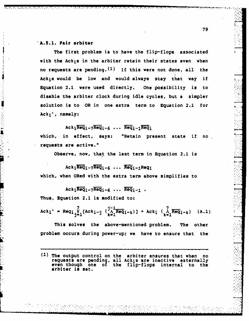
79

"A.5.1. Fair arbiter

The first problem is to have the flip-flops associated

with the Ackis in the arbiter retain their states even when

no requests are pending.(1) If this were not done, all the

Ackis would be low and would always stay that way if k

Equation 2.1 were used directly. One possibility is to

disable the arbiter clock during idle cycles, but a simpler

solution is to OR in one extra term to Equation 2.1 for

Acki', namely:

Ackik- i-7W- i-6... lei-lk- iwhich, in effect, says: "Retain present state if no

requests are active."

Observe, now, that the last term in Equation 2.1 is

" Ackike-7 7 - 6 . -.. 1ei-Reqi'-

which, when ORed with the extra term above simplifies to

Ackikeqi-71eqi-6 ... Teqi-1

Thus, Equation 2.1 is modified to:7j 7

Acki' - Reqijl(Acki-j (j*17i-k)] Acki (! A-qi-k) (A.1)

This solves the above-mentioned problem. The other

problem occurs during power-up; we have to ensure that the

(1) The output control on the arbiter ensures that when norequests are pending, all Ackis are inactive externallyeven though one of the flip-flops internal to thearbiter is set.

.0....77777

* .°.-• ,

so

arbiter initializes in a valid state, i.e., exactly one of

the flip-flops representing the Ackis should be set. This .

problem is solved by replacing Ack i in Equation A.1 by Ai,

where

....ECT Xc ijck i (i-0,1,...,6):

Ai - (A.2)ECoXC=T1 ... AcW6 (i-7)

It is easily seen that in a valid state (exactly one Acki

set), Ai and Ack i are always equal. In an invalid state, it

behaves as follows: If all Ackis are logic 0, A7 is high .-

and all the other Ais are low. If more than one Acki is

logic 1, only the Ai corresponding to the lowest numbered

one will be high. Note that after the very first clock .7

cycle, the arbiter will immediately enter a valid state and

will remain in valid states thereafter.

Thus, the final equation for the PAL is:

7 j-1 7Acki'-Reqij.lAAi- j A)] + A1 ( A Reqi-k) (A.3)

where Ai is as given by Equation A.2. Figure A.7 shows the

schematic diagram for the arbiter implemented on a PAL16R8.

A.S.2. Original arbiter design

Sections 2.3.1 and 3.6 refer to the "biased arbiter"

which was discarded in favour of the design in Section A.5.1

above. For reference, we give the equations corresponding

to the biased arbiter:

- . .' . .°.

81

Logic Diagram PALMOSIs*too

INPUTS (0-31)

A A . . . . . .. . .5 2 IIS S tI~ b l f .. lt*. .. a a

ReQ, S~ ~~~ill T i ll* lIII ISlI SIl,,nIl*ti

Fiur fill Scheati diga frabie ARAO-

Oak-

. -. . . . . . . . . .

. . . . . . . . . . . . . . . . . .

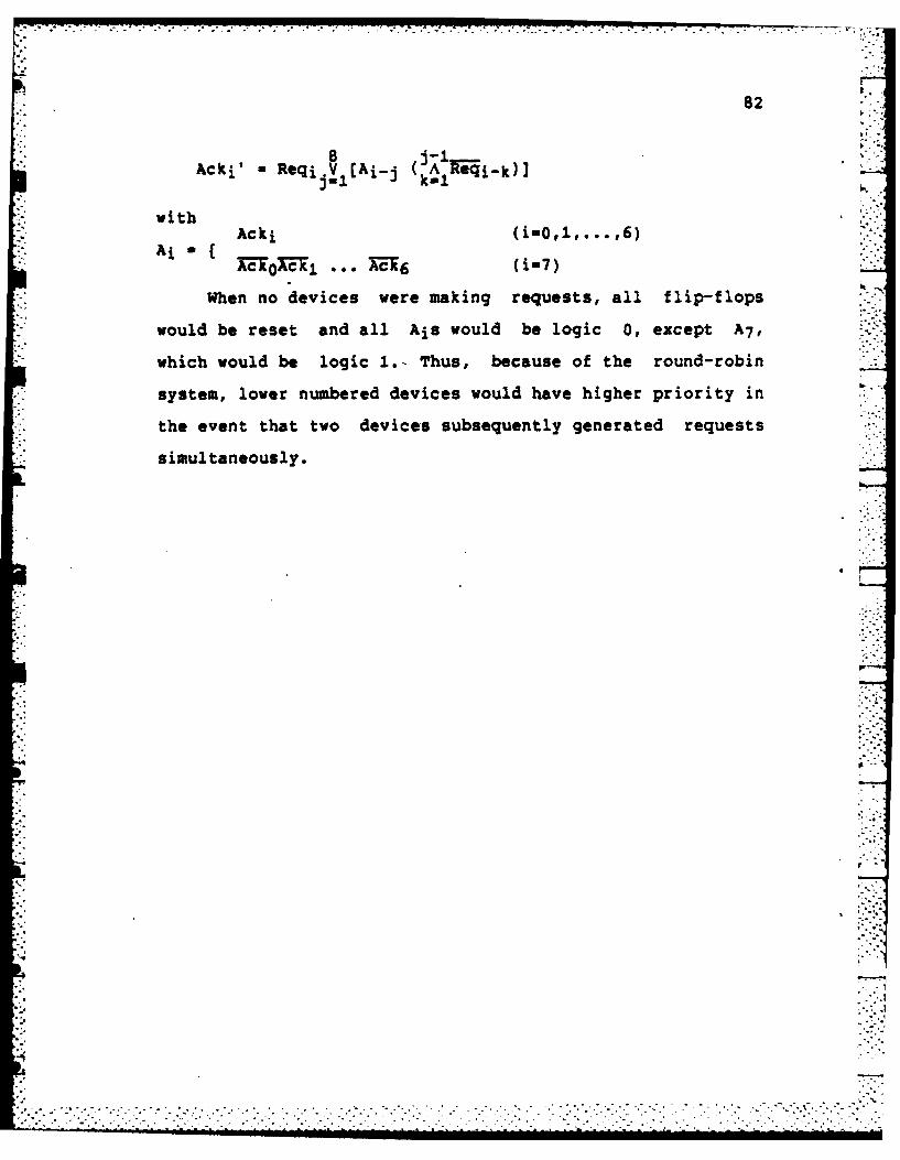
82

8 j-1Acki' *Reqi V ([A'j~ (k~ A ij-01

withAcki 10,. 6

A1 TX-T - _ ** (i=n7)

when no devices were making requests, all flip-flops

would be reset and all Ais would be logic 0, except A7,

which would be logic I.- Thus, because of the round-robin

system, lower numbered devices would have higher priority in

the event that two devices subsequently generated requests

simultaneously.

da ib, . . . . . ... . . .. . .. . .. . .

83

B. ANALYSIS AND SIMULATION SOFTWARE

B.1. Listing of program to calculate parameters for FCFS model

[$R+)program F i fo arbi ter;{

Author: Shahrukh MerchantDate: 14 May, 1984Last revised: 21 May, 198.

Language: "Turbo" Pascal Version 1.00 on the IBM Personal Computer

This program models the arbiter as a FIFO dicrete-time queue, and computesthe steady-state probability mass functions for (a) the number of customers(devices that have requested service) in the system and the waiting time(including service) of a customer.

Important variables used are:

N (constant) - Total number of devices in the system being simulated.NPI (constant) - N + 1.EPSILON (constant) - Magnitude of largest number that will be treated as

zero (due to round-off, etc.).p - probability of any inactive device making a request in a time slot

(o<p< I).pii] - steady-state probability that i devices are active (I customers are

in the system.tableau - transition matrix for system, augmented with an extra row and

column, and adjusted so as to facilitate solving the matrixequation pi - pi * P. If I and j are the initial and finalstates respectively, then let Pli,j3 - Probability of going fromI to j in 1 step.The system of equations we need to solve is:

pi * 1P- I *0 or IP- I (t) *p i -0pi t 1 ... 13 (t) I. 11 ... 1* pi - I

(The (t) symbol denotes the matrix transpose.)

So "tableau" has the form:

(t) 0

0-' - -: -- - - -

111. .1 1

and one of the equations is redundant.

choose[l,jJ - binomial coefficient (I,J) for 0 <- ij <- N (it is zerofor undefined combinations, e.g., (3,1)).

pexp[i] - i'th power of p, for 0 <a I <- N.Cp-expl3 - i'th power of (1-p), for 0< I <- N.

- . - .. .*

"'" ' ""- "a ** .*" ".. . . . . °.. .. ' ' " ' " "" ' "" - L i : : "-: ;,'-., , -. - .,--, .. ,', . .. - -' - - .-. . -.-. " . . .L . _ - -- : . .. - - - - - -"l "

84

wait,,pdf [i3 ProbabilIity that an arriving customer has to wait for time i(including service time) .

Begin main program declarations

const N - 8;NP1 - 9;EPSILON - .Oe-8;

var p. average, mean square :real;pi :arrayEO. N3 of real;tableau :arrayEO..NPI,O..NP1J of real;choose :arraytO..N,O..N3 of real;pexp cpexp :array[O..NJ of real;

I :integer;weaItpdf :array~l..NJ of real;answer :char;

Begin subprogram declarations

procedure pr int tabl1eau;

This is a DEBUGging procedure and simply prints out a dump of thearray tableau, row by row.

var i~j :integer;

beginfor i:- 0 to N+l do

beginfor J:- 0 to N+1 do write (tableau~i,J3);wr itel n

endend; (procedure print tableau)

procedure initialize;

This procedure initializes the following output variables/arrays(declared globally) to their required values.

Outputs: choose p exp cpexp tableau

Inputs: N, EPSILON, p

var lij :integer;total :real; (for DEBUGging only)

begin

85

Initialize "choose"

for 1:- 0 to N dofor j:in 0 to N do chooseti,jJ3:i 0;

-. chooseCO,OJ:in 1;for i:- I to N do

beginchooseti,OJ:in 1;for j:- 1 to N do choose(i~jJ:- choose~i-1,j-lJ + choose~i-I.j)

end;

Initialize pexp and cp~exp

p_*xp103:- 1; cp...xp[OJ:in 1;for 1:- 1 to N do

beg inp-4exp~iJ:- P..expti-1J P;cp-expli3:. Zp.., xp~i-lJ 0 (-p)

endr

Initialize tableau

for i:-O0 to N dofor j:-n 0 to N+l do tableaui,j3:in 0;

for J:- 0 to N+l do tableau[NHI,jJ:- 1;(Fill in non-zero transition probabilities)for pm- 0 to K do tableauti,OJ:- chooserff.j] p.xprj) *P cexp(N-j;

( row 0)for i:- 1 to N do

for J:- i-1 to N-1 do tableaulj,i3:- choose(N-i,j-i+lJp...expt-i+lJ cpexp(N-j-lJ; (other rows)

{DEBUG CODE BEGIN) (Check for stochastic matrix)for i:- 0 to N do

begintotal: 0;for j:- 0 to N do total:- total + tableau~j,i];if abs(total-l.O) >a EPSILON then

beg inwriteln ('*** ERROR: Column'. i:4., is not stochastic.',

Tableau reads:');

p~rint tableau; haltend

wrtand; *Sohsi es ucsfl*)

(DEBUG CODE END)

(Subtract out identity matrix)for ;:a 0 to N do

beg intableau[l,1J:- tableau~i,1J I

endend; (procedure Initialize)

86

procedure solve;

This procedure carries out Gaussian elimination with back substitutionon "tableau" to obtain the pi vector. Scaled partial pivoting is usedto reduce round-off error. See S.D. Conte & Carl de Boor, "ElementaryNumerical Analysis: An Algorithmic Approach," McGraw-Hill, 1972.

Inputs: N, NPl, EPSILON, tableau4

Outputs: pi, tableau (destroyed)

var size :arraytO..NP13 of real; (used in pivoting strategy)index, I. J. k :Integer;factor, max, temp :real;

beginfor k:- 0 to N do (for each variable)

begi nfor i:- k to W+ do

begi nteap:- 0;for J:in k to N do temp:-n temp + abs(tableaui,jJ);sizeti3:- temp

end;max:- 0; index:- -1;for i:- kt to 14+1 do

b~eg I ntemp:- abs (tableau~i~kJ);if slzetiJ > EPSILON then

if temp/sizeti3 >- max thenbeg inmax:- temp/s 1261i3; -..

Index:- Iend

end;

(DEBUG CODE BEGIN)if index - -1 then

beginwriteln ('*** ERROR: Zero pivot element at step', k:4, 'Tableau is:');print tableau; halt

end;(DEBUG CODE END)

(Exchange rows)if k <> Index then

for J:- k to N+l dobeg intemps.- tableau~k,j3;tableau~k,J3:- tableautindex,jJ;tableauindex,jJ:. temp

end;for l:in k+l to W4 do

-7

87

beg infactor:- tableau~i,kJ/tableau~k,kJ;tableau~i,k3:- 0;for j:-n k+1 to N+l do

tableautij3:- tableauti,j3 factor *tableau~k~jJend

end; Nk loop)

{DEBUG CODE BEGIN)writeln ('* Pivoting complete W');(Verify that one equation was redundant (last raw 0))if abs(tabieau(N+1,N41J) >- EPSILON then

begin ---

writeln ('*** ERROR: Redundant equation inconsistent. Tableau reads:');printtableau; haltend

else writeln (1* One redundant equation. O.K. *1);(DEBUG CODE END)

Back substitution to get pi vector

for i:- N downto 0 dobeg intamp: - 0;for J:- i41 to N do temp:- temp + tableau~i,j3 *ij3piil):- (tableauti,N41J - tWmp)/tebleaui.iJ

end;

(DEBUG CODE BEGIN)(Recreate transition matrix (use tableau for storage) and ensure thatpi-pi*P is satisfied and that the pil13's sum to 1.)

(Check Pi Li's sum to 1)tempfin 0;for i:w 0 to N do tamp:- temp + piti);if abs(temp-1.0) >- EPSILON then

beg inwrlteln '**ERROR: pi[IJ''s do not sum to unity. pi vector is:');for 1:-n 0 to N do write (pi [i);writeln; haltend

also wrltein (C* p003"s sum to unity. O.K. *');

(Recreate transition matrix)for 1:m 0 to N+l do

for j:- 0 to N44- do tableauti,j):- 0;for j:n 0 to N do tableau[OJJ:- choosetN,J] * pexp~] * cp exp[N-JJ;for Hun 1 to N do

for J:in i-1 to N-1 dotableaui,jJ3:n choose[N-i,j-i+13p p.exptj-i+13 cp exp[N-J-13J;

(Check for plmpi*P)for J:m 0 to N do

88

beg intemp:i 0;for Ito 0 to N do tamp:- temp + PiEil tableauti~jl;if abs(piU)]-temp) >- EPSILON then

beginwritein ('*** ERROR: pi-pi*P not satisfied. pi vector is:'); .-for i:in 0 to N do write (pitiJ);writein; writein ('Transition matrix Is:');

adprint-tableau; halt

and;writein Q'* pimpl*P is O.K. *')(DEBUG CODE ENDS)

end; (procedure solve)

procedure waiting time;

This procedure computes the waiting time probability mass function.The waiting time will always be in the range I to N inclusive.

Inputs: pi, N, choose, pexp, cp~exp. p. EPSILON (DEBUG only)

Outputs: Wait-Odf

var I.s.gj :Integer;SLOP :real;

beginfor l:-n 1 to N do

beg inwe! tpdf113:- pi[03 choose[N,13 * xp113 cp,.exp[N-i);for *:- 0 to I do

beginSum:- 0;for g:- i-s+1 to N-s do sum:n sum + chooseEN-s,gJ pe*xp~gJ

*cp *XPEN-S-gJ;walt-pdf l3s- wait,.pdf Liii D ifsJ sum

end;

sum:- 0;for J:- 0 to N-1 do sum:- sum + pi[J3 (N-i);wait.pdf i:. walt-pdf~iJ/(p*sum)

and;

(DEBUG CODE BEGIN)(Check that probabilities sum to 1)Sum:.' 0;for it= 1 to N do sum:- sum + waitjpdf [13;If abs(sum-1.0) >= EPSILON then

wrltaln (**ERROR: Waiting-time probabilities do not sum to 1'

........... '....%~ -.. . .. . . .

89

else writeln (1* Waiting time probabilities sum to 1. O.K.*)

(DEBUG CODE ENDS)

end; {procedure waitingtime)

BEGIN AIN PROGRAM

beginrepeat

write ('Enter request probability: '); readin (p);Initialize;

solve; (solve tableau for steady-state probability vector pilwriteIn; writeln ('Steady-state probability vector is:');- writein;average-i 0;for i:- 0 to N do

beginwritein ('pit', i:2, '3 1 , pOEiM;average:u average + i It pi~i3

end;writeln; writeln ('Average number in system inaverage);

waiting time; (compute waiting-time probability mass function)writeln; writein ('Waiting time probability vector is:'); writeln; --

average:- 0; mean square:- 0;for i:- I to N do

beg inwritein ('w[', i:2, '13 1, waitpfti]);average:- average + I It wait pdfTi3;meansquare:- mean square + i~qr(l) It w i t-O.pf I 1

end;writeln; wrlteln ('Average waiting time -n', average, ', Variance -n',

mean square - sqr (average));

write ('Restart (R) or Quit (Q) ?')readi1n (answer); answer:- upcase (answer)

until answer <>IR

end. (program Fifo-arbiter)

90

8.2. Simulator listing

{$R+1program Arbiter-simulate;{

Author: Shahrukh MerchantDate: 21 May, 1984Last revised: 21 May, 1984Also revised: 21 June. 1984 to include "Fair" arbiterRevised 24 June, 1984 to include unequal request probability for device 1.Revised 25 June, 1984 to allow general file I/O.Revised 2 July, 198 to allow variable (integer) idle Ion (formerly

always 1).Revised 6 July, 1984 to include First-come, First-served (FCFS) arbiter.

Language: "Turbo" Pascal Version 1.00 on the IBM Personal Computer

This program simulates the arbiter as a discrete time round-robinqueue, to determine the probability mass functions of:1) the number of customers in the system2) the waiting time of a customer3) the length of a busy period and4) the length of an idle period.

Three types of arbiters are implemented:1) A "Fair" round-robin arbiter2) A "Biased" round-robin arbiter and3) A First-come, First-served arbiter.

See the discussion in the text of procedure next device for a descriptionof the first two. The third is a simple FCFS queue, with random selectionin the case of simultaneous arrivals.

The waiting time distribution is determined separately for each customeras well as for the whole system.

Request generation can be a function of a) the device number andb) the number of cycles since the device was last served (including 0).Therefore, it does not have to be the same for all devices, nor does ithave to have the same constant probability per cycle for every inactive -device. However, a device that has a request pending cannot generateanother request. The request generation is governed by the function -."pr req" and the procedure "initprreq.".

Important variables used are:infile, outfile - Input & output file variables, respectively. ;ft....N (constant) - Total number of devices in the system being simulated.MAX)BUSY, MAX-IDLE (constants) - Maximum busy and idle period lengths,

respectively, that we want to keep track of in their respectivedistributions.

clock - count of number of cycles of simulation (a real number sinceintegers only go up to 32767.

dev idleti3 - length of current idle period for device i (set to zeroIf not idle).

" . . . .i..... :............. .l. ~ - -1- . . 2 . .. . . . . ... ... -- . .

91

n-cust - Number of customers currently in system (making requests orbeing served).

request[i] - "true" if device i is currently making a request. "false"otherwise.

current dev - device currently being served (0 if no device is beingserved).

last_dev - device currently being served, or last device served if nodevice currently being served. Used only for "Fair" arbiter.

dev.wait[i] - current waiting time for device i (0 if device i is notcurrently requesting).

wait pdf[i,j3 - number of times during simulation that device i waitedfor time j (1 <- i.j <= N).

n custpdfi] - number of simulation cycles that the number of customersin the system was 1.

busytime - number of cycles that system has been continuously busy (0 ifsystem idle).

idle time a number of cycles that system has been continuously idle (0 ifsystem busy).

idle len - number of cycles after a request for a particular device hasbeen served that that device is guaranteed to be idle (i.e., willnot generate a request).

busy-pdfCi - number of busy periods of length i (1 <- i <- MAX BUSY).busypdfO is used to store the number of busy periods of length> MAX BUSY.

idle pdfCIl - number of idle periods of length i (1 <- i <a MAXIDLE).idlepdfCO3 is used to store the number of idle periods of length> MAX IDLE.

longest busy, longest idle - longest busy and idle periods, respectively,encountered during simulation.

n busy, nidle - number of busy and idle periods, respectively,encountered during simulation.

dev req113 a number of requests serviced for device i during simulation.iter limit a maximum number of iterations for which simulation is to run.busy limit m maximum number of busy periods for which simulation is to run.arbiter type - 'F' if "Fair" arbiter is being used, '8' if "Biased"

arbiter is being used, '1' if FCFS arbiter is being used.queue[O..NJ - array containing queue of request arrivals. It can contain

at most N elements (i.e., if all devices are requesting). Used onlyfor "FCFS" arbiter.

queue head a points to top-most element of "queue." Used for "FCFS"arbiter only.

queue tall a points to element following bottom-most element of "queue."If queue is empty, queue head-queue tail. Used for "FCFS" arbiteronly.

sum busy, sum idle - sum ofalengths of all busy and idle periods,respectively, during simulation.

sum busy sq, sumjidlesq - sum of square of lengths of all busy and idleperiods, respectively, during simulation.

(These last 4 variables are used to determine the mean and variance ofbusy and idle period lengths. This cannot be determined exactly fromtheir probability mass functions busypdf and idle pdf because the

• ' ,, ..'--- .-.. ". . . . . " "-- -i . -...-- - . ..- - .. , ---- ,

92

latter are truncated beyond MAX BUSY and MAX-IDLE respectively.)

Begin main program declarations

const N - 8;FIAX BUSY - 500;MAX IDLE - 500;

type range O..N;small-range - I..N;

var infile, outfile :text;n-cust, current.dev, last dev, queue-head, queue-tail :range;idle Ien :integer;

p1, p, clock, busy time, idle time, n busy, nidle,sumbusy, sum idle, sumnbusysq, sum idle.sq,iter limit, busy_limit, longest-busy, "-I ongds ti die :rea;

dav Idle, dev.req :array[l..N] of real;request :array[l..N3.of boolean;dev wait :array[l..NJ of range;nqcustpdf :array[O..N3 of real; . -busyipdf :array[O.. AXBUSY of real;idlepdf :array[O../AXmIDLE] of real;wait_pdf :array[l..N,l..N3 of real;queue :array[O..N3 of small range;

answer, arb i tertype :char;

Begin subprogram declarations

procedure io;

Determine input and output files/devices O

var filename :string[143 ;

beg i nwrite (con, 'Input file (use CON: for console input): ');

("con" is a pre-declared text-file variable for console I/0) IreadIn (con, filename);assign (Infile, filename);reset (infile);

write (con, 'Output file (use CON: for console output): ');readIn (con, filename);assign (outfile, filename); rewrite (outfile)

A1

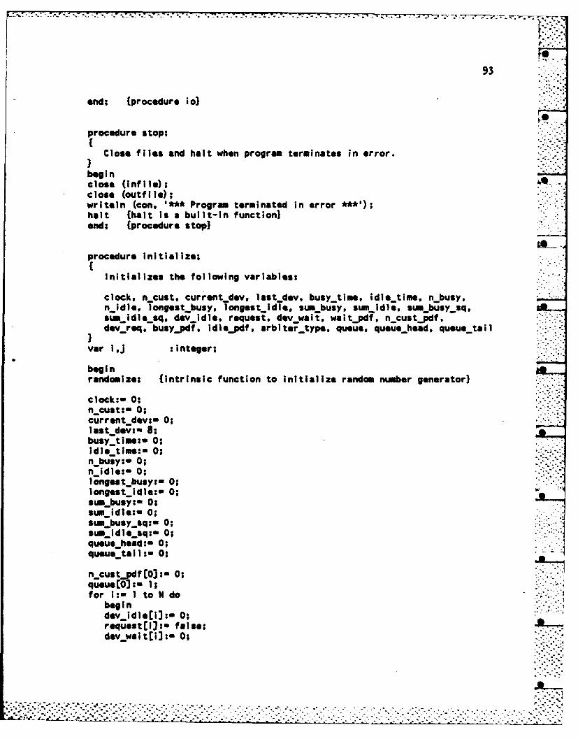
93

end; (procedure iol

procedure stop;

Close files and halt when program terminates in error.

beg inclose (Infile);Aclose (outfile);writein (con, '*** Program terminated in errorhalt (halt is a built-in function)end; (procedure stop)

procedure Initialize;

Initializes the following variables:

clock, n-cust, currentdev, lastdev, busy tim, idle-time, n-busy,n idle, longestbusy. longestidie, simbusy, sum idle, sumbusysq,*;Pmidle-sq, devidle, request. dayvwait, waitjdfT, ncustjdf.devreq, busy_.pdf, ldlejpdf, arbitertype, queue. queue head, queue tail

var 1,j :nteger;

beg inrandomize; (intrinsic function to initialize random number generator)

clock:- 0;n cust:- 0;,current dev:- 0;last-de:n 8;busy-time:- 0;idle time:- 0;n-busy:n 0;n idle:- 0;longest-busy:- 0;longest idle:- 0;sumsbusy:- 0;sumkIdle:* 0;sumRbusy~sq:n 0;suIidle sq: - 0;queuehead:.- 0;queuetall:- 0;

n cust pdfEO3:s 0;,q;ueeEOJ:- i;for I:- I to N do

beg indev idle[13:- 0;roquest~i):a false; *Y9

dey..wa It iJ:- 0;

9'.

n cust-pdf [I):- 0;queueciJ:. 1;dev req~iJ:- 0;for j:- 1 to N do wait~pdfti,jJ:ft 0

for 1:- 0 to MAX BUSY do busy..pdf El):- 0;for i:- 0 to MAX IDLE do idle.,dfti]:m 0;

repeatwrits (con, 'Fair(F), Biased(S) or FCFSMl arbiter ? ');readin (infilie, arbiter type); arbiter type:- upcase (arbiter type)

{upcase Is built-in function)until arbltertype in C'F','B'.'l'J

end; (procedure initialize)

procedure initprreq (var idle-Ion :integer; var p1, p :real);

This procedure initializes all those parameters used by the functionprreq that are use*d to compute request probabilities.If these paramters are changed due to a change in the form of functionprreq, the following changes must be made to the rest of the program:1) Remove the declaration of all parameters that are no longer used

from the declaration of variables In the main program, and from thecomments describing the use of all variables.

2) Add the declaration of all new parameters to the main programdeclarations, and to the comments describing the use of variables.

3) Change the parameters of initprjreq where it is invoked by themin program and elsewhere.

4) Remove any other references to these parameters elsewhere in theprogram.

Outputs: p (the probability that any inactive device (2-8) will make arequest for any cycle other than the one immediatelyfollowing a &arvice completion of that device)

p1 (same as above for device 1)idleIen (nuber of cycles after completion of a service for a

device that that device is guaranteed to be idle).

beginwrite (con, 'Enter number of guaranteed idle periods:')readln (infile, Idle Ion);write (con, 'Enter device request probability (dev 1): 1);readin (inflle, p1);write (con, 'Enter device request probability (dev 2-8): ');readIn (infile, p)a nd; (procedure itprreqj

95

procedure input (var Iter limit, busy limit :real);{--This procedure initializes those variables that control the runningof the simulation.

beginwrite (con. 'taxImuI number of Iterations ? );readin (infile, Iter limit);write (con, 'Maximum number of busy periods ? );readin (infile, busy limit)end; (procedure input)

function prreq (devnum :Integer; dev-idle.time :real) :real;

This function generates request probabilities greater than or equalto 0, and less than V, for a device (number devnum) to make a requestfor the next cycle, given that it has been idle for a certain numberof cycles already (devjdle-time)"

This function needs to be "customized" for different cases.Rewriting and recompiling can be avoided to a certain extent by usingprocedure init pr-req to initialize parameters used by this function,If all one needs to do is to change parameters without changing theunderlying structure.

Note: While this procedure, and the simulation program in general,allows non-zero probabilities for a device for a slot (cycle)Immediately following the one In which It got served, the actualhardware being simulated could never allow a request for a cycle tobe generated while it is being serviced, so the same device couldnever be serviced for 2 consecutive cycles.

Inputs: Device number, cycles since last request completed, p, N

begin

(DEBUG CODE BEGIN)if (dev idle time -- 0.5) or not (devn um in I1..NJ) then

beginwriteln (outfile, '*** ERROR: Invalid Idle-time', devjidle time,

for device', dev num);stop

end;(DEBUG CODE END)

If dev.idletime 4- idlelen - 0.5 thenprreq: 0

else"-. .

if dev nuol thenprreq:n p1

elseprreq:- p

* ...... . .--- -- - - -

,.._,.:. ..- :. --._. ,- . .: . . .,.-.. ::::::::::- :::... . . . . . . . . . . . . . . . . . . . . . . . .-;.> ;-' - "''.- " "./ .-.- ',','.-,-.-..'.- .. ,'.-., .-- ,-..-. . . . .-.- . ....--. ... .- - - - , - :;:":

96

end; (function prreq)

procedure compute requests;

This procedure computes requests for every device, based on howlong that device has been Idle.For the FCFS arbiter, if simultaneous requests occur, they arerandomly shuffled.

Inputs: request, N, arbiter type, queue, queue head, queuetailOutputs: request, dev idle, queue, queue taillCalls: prreq

var i :small range;temp, count :range;shuffle :array(1..A3 of salIIjange;

begincount:- 0;for I:- I to N do

if not requesti thenbeginrequest~iJ:- random -c- pr req(I,dev idle[lJ);- {random is a

built-in function that returns a random numberin the range (0,1))

if request[13 thenbegindev idletl]:- 0;if arbitertype - IV then

beg incount:- count + 1;shuffletcount]:- I (Store requests)

endend

end;

If arbiter type - 1' then (update request queue if FCFS)for I:= count downto 1 do (Shuffle them)

beg intamp:- random(i) + 1; (Random(i) returns random integer

between 0 and i-I inclusivequeue~queue ta 1]:- shuffle~temp];shuffletteu~p3:- shufflel];If queue-tail >- N then

queue-tail:- 0else

queuetaiI:* queue-tall + ;(DEBUG CODE BEGIN)If queuaetall - queuehead then

beg inwritein (outfile, '*** ERROR: Queue pointers both equal',

queuetall, after request for dev', 1);

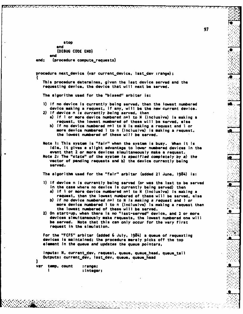
... : - -o97

stopend(DEBUG CODE END)

endend; (procedure computerequests"

procedure nextdevice (var current-device, last-dev :range);

This procedure determines, given the last device served and therequesting device, the device that will next be served.

The algorithm used for the "biased" arbiter is:

1) If no device Is currently being served, then the lowest numbereddevice making a request, if any, will be the new current device.

2) If device n is currently being served, thena) if 1 or more device numbered n+l to N (inclusive) is making a

request, the lowest numbered of these will be served, elseb) if no device numbered n+l to N is making a request and I or

more device numbered I to n (inclusive) is making a request,the lowest numbered of these will be served.

Note 1: This system Is "fair" when the system is busy. When it isidle, It gives a slight advantage to lower numbered devices in theevent that 2 or more devices simultaneously make a request.

Note 2: The "state" of the system is specified completely by a) thevector of pending requests and b) the device currently beingserved.

The algorithm used for the "fair" arbiter (added 21 June, 198) is:

1) If device n is currently being served (or was the last to be servedin the case where no device Is currently being served) thena) if I or more device numbered n+l to N (inclusive) is making a

request, then the lowest numbered of these will be served, elseb) if no device numbered n+l to N Is making a request and I or

more device numbered 1 to n (inclusive) is making a request thenthe lowest numbered of these will be served.

2) On start-up, when there is no "last-served" device, and 2 or moredevices simultaneously make requests, the lowest numbered one willbe served. Note that this can only occur for the very firstrequest In the simulation.

For the "IFCFS" arbiter (added 6 July, 1984) a queue of requestingdevices Is maintained; the procedure merely picks off the topelement in the queue and updates the queue pointers,

Inputs: N, current_dev, request, queue, queuehead, queue tailOutputs: current.dev, last dev, queue, queuehead

var temp, count :range;I :Integer;

_____________________________"_____________ ° .-.. > :...o:.

98

beg i nif arbitertype III1 then

beginif queue head queuetail then fempty-no pending requests)

current-dcv:- 0else (get topmost element in queue and update pointers)

begincurrentdOev:- queue tqueue~headj;If queue-head >- N then

queue-head:- 0else

queue head :- queue head + 1;last dev:- currentdev

endend

else (IF' or 'B' arbiter)begi nIf arbiter-type I F' then

i:- last develse

I:-n current dev;temp:- 0; count:- 0;repat

I:w I + 1; if 1-11+I then 1:- 1;count:= count + 1;If requesti3 then temp: - I

until (temp-l) or (count-N);current-dev:- temp;if temp <> 0 then last dev:- temp

endend; (procedure nextdevice)

procedure update; -

This procedure updates all variables that need to be updated afterevery simulation step, for keeping track of various parameters.

Updated variables (i.e., Input and output):clock, request, dev wait, devidle, Idle-time, busytime. n-busy,nidle, sumbusy. sumidle, sum busysqo stuulidle* sq, busypdf,Idlepdf, waitpdf, dev req, longest busy, longest idle, n custpdf

Other Inputs: N, MAXSBUSY, MAX-IDLE, currentdevOther outputs: ncust

var I, temp :integerl

beginclock:- clock +9 1;

(Compute number of customers)n-cust:- 0;

99

for i:- I to N doif requesti then

beg inncust:n n cust + 1;dev waitlT:' dev._wait[13 + 1and-

elsedevildl*EC3:- day .idle[iJ + 1;

n-custjdtf En~custj :1 p~custjdf (n..custj + 1;

(Do busy and Idle times now)If n cust a 0 then (no customer to be served)

begIn(DEBUG CODE BEGIN)If current,_dev 4b 0 then

beg inwritein (outittle, **ERROR: n cust p-'cnust, but current dev i'

current~dev);stop

(DEBUG CODE END)if Idletims 0 then (Just became idle)

begin(nw CODE "GIN)If (busy-time - 0) and (clock -c 1) then

beg inwritein (outfile, '*** ERROR: idletime S busytime both 0',

at clock-'., clock);stop

end;(DEBUG CODE END)If busytime <> 0 then (false at clock-i only)

beginnbusy:- n busy + 1;sum-busy:- s&Rmbusy + busytime;,suxibusy sq:- sumbusysq + sqr (busy time);if busytIme >- longest busy then longestbusy:- busy time; '

If busy time <- MAX BUSY thenbegintamp:- round (busy time);busypdf tep3:- busypdfEteMPj + Iend

elsebusypdf E03 :- busypdf (0) + I

end;busytime:- 0

end;idletime:- Idle time + 1;(DEBUG CODE BEGIN)If round(busy-time) 4:1 0 then

beg inwriteln (outfile, '*** ERROR: busy time ibusytime,

Iduring Idle period');

100

stopend(DEBUG CODE END)end (" If n cust-01)

else fn cus t 0o o0- customers to be served)beg in(DEBUG CODE BEGIN)If current dev - 0 then

begin Opwritein (outfilie, '*** ERROR: n cust n. cust, but current dev '

current, dev);stopend

else If not request~currentdev3 thenbeginwriteln (outfile, **ERROR: requestL', current-dev:2, ' false');stop

end;(DEBUG CODE END)if busytIm. - 0 then (just bece busy)

begin(DEBUG CODE BEGIN)if (id4etime -0) and (clIock *1) then

beg inwriteln (outfile,'*** ERROR; idletime and busy time both zero at'*

clock -1, clock);stop

end;(DEBUG CODE END)If idle time <> 0 then (false at clock-I only)

begI nn Idle:- n Idle + 1;sumidle:- sum-idle + idle-tim;sumviIesq:- sum~idles*q + sqr(idletime);If Idle time 31- longest idle then longest idle:- idle time; .if idle time <- AAXIDLE then

begintamp:. round (ldle-time);I dle*jdf tuipJ - I dejdf EtSMP3 + 1end

else ll.pfO

end;Idletlme:- 0

end;busytime:- busy time + 1;(DEBUG CODE BEGINIf round Cidle time) -c 0 then

beg inwritein (outfile, '*** ERROR: IdletIme inidletIme,

during busy period');,stop

101

end;(DEBUG CODE END) .k.(Now do waiting times)tamp:- dev wai t~current dev]; -

wal t~pdf Ecurrent dev, temp] : wai tpdf Icurrent..dev, temp] + 1;dev wal t~current dev :- 0;dev.,req~current devj :- dev req (current-devj + 1;request~currentdevj :- fals;e (service completed)

end (else clause of "if n cust -0)end; (procedure update)

procedure output;

This procedure outputs the result of the simulation.

Inputs: N, MAXBUSY, MAXIDLE, n custpdf, clock, dev req, wait-df,sumbusy, nbusy. sum busysq, sumidle, nidle, sum idle sq,longestbusy, busypdf, longest-idle, idlepdYf, arbitertype, pt pi,idle-len

var i Vj : range;totreq, tempt sum, average,mean square :real;answer :char;count, limit :integer;

beg inwritein (outfile, 'Arbiter type - ,arbiter type,

Req. prob. (dev 1) m'.pl:S:5, ' Rieq. prob. (dev 2-8) i P:8:5)'.writeln (outfile, 'Guaranteed idle length -n', idle len:I.);writein (outfile, 'Distribution of -number of custom;ers:');average:- 0;for Hatn 0 to N do

beg intamp:-, n cust..pfti3/clock;writeln loutfile, 'PIP', 1:2. '1 ' temp);average:-n average + I * tamp

end;writeln (outf 11., 'Average number in system -1, average);

writeln (outfile, 'Distribution of welting times:');totrq:in 0;for I:- I to N do tot-req:in tot-req + dev-reqli3;average:- 0; meansquare:- 0;for J:- I to N do

begi1nsum:- 0;for i:-n 1 to N do sum:- sum + wait-pdf (i~j];tamp:- sum/tot req;writein (outfle, 'w[1, J:2, '1 a$ tamp);average:-n average + j *tamp;

p. 102man square:- mean square + sqr Q) *temp

end;writeln (outfile, 'Average waiting time -n', average, ', Variance i'

mean-square -sqr (average));

repeatwrite (con, 'go you want waiting-time distributions',

for each device ? ');readin (infile, answer); answer:w upcase(answer) fupease is built-in

function that converts a character to upper case)until answer in ['Y',WN';if answer - 'Y' then

for I:- 1 to Ndobeg inwritein (outfile, 'Device #,1:2, K

* ',dev reqtiJ:8:0, ' requests)');if dev reqliJ 0 then

writein (outfile, '*** No requests for device', i:2,'else

beginIL average:- 0; mean square:- 0;

for J:in 1 to N dobegintemp:-n waitpdfi ,jJ/dev req[ij;writein (outfile, 'win, N:29 T(, Z:. '1I' temp);average:- average + j * tamp;meansquare:- meansquare + sqr C]) * tamp

end;wrlteln (outfile, 'Average -1, average, ', Variance '

mean-square -sqr (average))end

end;

if n busy <- 0.5 thenw riteln (outfilie, 'Less than 1 busy period; cannot compute average')

elsewritein (outfile, 'Busy time: mean -', sum busy/n busy, ' variance '

(nbusy * sum-busysq - sqr (supmbusy)) /sqr (n-busy));

if n-idle <- 0.5 thenwritein (outfile, 'Less than I idle period; cannot compute average')

elsewritein (outfile, 'idle time: mean -1, sum idle/n idle, ' variance '

(n-idle * sum-idle-sq - sqr(sumiIdle)) / sqr(n~idle));

repeatwrite (con, 'Do you want busy/idle time distributions ?')readl n (Infi le, answer); answer:- upcase (answer)

until answer In E'Y','N');If answer - 'Y' then

beg inwritein (outfile, 'Busy time distribution: ');If longest-busy >- 14AXDUSY then

103

limit:- MAX BUSYelse

limit:- round(longest busy);for count:- I to limit do

writein (outfile, 1b[', count:., 'J -n', busypdftcountJ/n busy);writein (outfile, 'Longest busy period -1 longest busy);writein (outfile, 'Number of busy periods with length >', MAXBUSY:5,

is'. busyjpdf[0J);

writein (outfile, 'Idle time distribution: 1);if longestidle >- MAX-IDLE then

limit:- M4AX IDLEelse

limit:- round (longest idle);for count:- I to limit do

writeln (outfile, 'i[', count:1., I ' idle pdf~countJ/n idle);writeln (outfile, 'Longest idle period alongest-idle);writeln (outfile, 'Number of idle periods with length >1, tAXIOLE:5,

Is', iIlepdf10])endend; {procedure output)

BEGIN MAIN PROGRAM

begi n*io; (initialize input/output. devices)* repeat

Initialize;initprreq (idle len, p1, p);

repeatinput (iter limit, busylimit);

repeatcompute requests;next device (current dev, last dev);update;if frac(clock/1O00) <- 0.0001 then

wrlteln (con, 'iteration', clock:8:0, ', Busy periods-'n busy:8:O)

until keypressed or Iclock >- iterjlimit) or (nbusy >- busylimit);(keypressed is built-in function; returns true if any key pressed)

repeatwriteln (outfile, '**Simulation complete **)wrlteln (outfile, 'Iteration', clock:8:0, ', Busy periods '

n busy:8:0);write (con, 'Output 70), Continue (C), Restart (R) or'

Quit (Q) ? ');read In (lnf ile, answer); answer:- upcase (answer);If answer - '0' then output

until answer In ['C','R','Q'J

104

until answer In E'R.,'Q'3

until answer-SQwritain (con, ^G, '**PROGRAM COMPLETE**9close (infile);close (outfile)

and. (program Arbiter-simulate)

ALI