1

8. The Theory of the Firm – Cost In this chapter you will learn: Short run costs;

Long run costs; Cost minimization; Scientific management; Competing with Japan and Europe; Business financing; Uncertainty and the firm’s decisions.

8.1 Short Run Cost The technology and organization of the firm implies a cost structure for the firm, both in the short run and the long run. First we'll consider the short run cost structure which governs the firm's choices in the short run. Then we will study the long run cost structure and relate it to the short run structure. This will give us a rich theory of the firm that will enable us to discuss how an industry adjusts to changes in the market place.

Our way of capturing the manner in which firms are organized and the engineering science behind their production is through the abstract notion of a "production function" studied in the last chapter, Y = F(L, K). If there is a technological breakthrough, the F( ) function will change. If the firm organizes itself more efficiently, the F( ) function will change. For example, prior to deregulation, most airlines would fly most of their passengers on direct flights. Unfortunately, this meant that many airplanes were mostly empty. Flying planes that are mostly empty is very costly for the airlines. However, since deregulation most airlines use a hub-and-spoke system where they fly most of their passengers to a hub airport, everyone changes planes, and then flies to their ultimate destination. This increased the occupancy rate dramatically and improved the airlines' profitability. We could model this as a change in the F( ) function.

In the short run we imagine that the way the firm is organized and the engineering science is fixed. In addition, we also assume the firm's capital investment is fixed as well. Suppose the firm has made an investment in the past that fixes its capital stock at K*. Output can be adjusted according to Y = F(L, K*). The only way for the firm to adjust its output in the short run is to adjust its labor input. When the firm begins using more labor, output increases a lot and we may actually observe increasing marginal returns (IMR) to labor. This occurs in the diagram below in region 0 - A on the total product curve. However, eventually, diminishing marginal returns (DMR) set in and less extra output is produced for the same increase in labor. This occurs in region A-B. It is even possible that too much labor has been hired, workers are distracting one another, bumping into each other, and so on, and output actually falls. This occurs to the right of point B where Y falls when L increases. However, no profit maximizing firm will ever operate in that region. The marginal product is just the slope of the total product curve. In region 0-A the slope is positive and increasing so the MP curve is positive and upward sloping. In region A-B the total product curve has positive slope but the slope is decreasing. This corresponds to region A-B for the MP curve. The total product curve reaches a maximum at B where its slope is zero. That's why the MP curve crosses the horizontal axis at B. Finally, the slope of the total product curve is negative beyond B. That's why the MP curve is below the horizontal axis beyond point B. This gives us the following product curves.

2

This pattern is very typical in a broad variety of companies. So it is important that we study

it. Keep in mind : high productivity corresponds to low cost on average and low productivity corresponds to high average cost. In region 0-A, productivity is very high so we expect short run cost to be low on average or falling in that region. In region A-B productivity is not quite so high so we expect average cost to be rising there.

The short run cost curves are derived from the total product curve. Imagine flipping the axes

to obtain the middle diagram above. Note that the regions match up. Then re-scale the vertical axis by multiplying by the wage rate. The diagram is elongated if w > 1 and it compacts if w < 1. On the far right we have the variable cost curve. It instructs the firm as to what its labor cost will be for each level of output. Higher levels of output require more labor and this increases the firm's variable cost. No firm will operate in the region beyond B*. Y* can be produced at cost C or D, but D is clearly inefficient.

The firm's fixed cost is given to it. One concrete way to think about fixed cost is as

mentioned : the firm has borrowed money to invest in building its factory and it must make monthly loan payments. This payment occurs whether or not the firm produces anything so it is constant relative to the firm's own production, as depicted in the middle diagram above. Other examples include property taxes, insurance on the plant, and depreciation of the plant and equipment. Finally, to get the firm's total cost in the short run add the variable and fixed costs

Y

L

Total Product Curve

0

A

B

MP

L

A

B

Marginal Product Curve

IMR

DMR

IMR

DMR

•

•

•

•

Y

L0

L

Y0

wL=VC

Y0

A

B

A

B

Variable Cost Curve

TP

• •

••

•

• C

D

B*•

Y*

TP

Totalproductcurve

wL=VC

Y Y Y

rK*=FC

rK* rK*

C = wL+rK*

Variable Cost Fixed Cost Total Short Run Cost

C

3

for each output level. This is depicted in the third diagram and it involves vertical summation. Therefore, the shape of the Total Cost curve is determined by the total product curve. Any change in the total product curve will lead to a shift in the firm's total cost curve. For example, if the firm invests in more capital, K** > K*, the total product curve will swivel up and the cost curve will shift upward as depicted above.

Another set of cost curves can be derived from the total cost curve, the marginal cost and the

average cost. In fact, the marginal cost (MC = ΔC/ΔY) is the slope of the total cost curve. These are depicted in the diagram, where the label prefix SR denotes "short run." This relies on the following definitions: MC = ΔC/ΔY is the marginal cost, AC = C/Y is the average cost, and wL/Y = VC/Y = AVC is the average variable cost. The "U-shape" of the short run cost curves reflects the shape of the total cost curve. Since the total cost curve reflects the total product curve and hence the productivity of labor, the short run cost structure of the firm also reflects the productivity of labor. The cost structure gets its shape from the technology and its first increasing marginal returns of labor followed by the decreasing marginal returns to labor. The MC curve will always intersect the AC and AVC curves at their minimum point.1

Short Run Cost Structure of the Firm

What did we hold constant in deriving the short run cost structure of the firm? The

technology, the wage (w), the cost of capital or interest rate (r), and the amount of capital (K*). If any of these variables change, then the short run cost structure of the firm will shift around. For example, if either the wage or the interest rate increase, the cost structure will shift up and 1 An easy way of relating the average variable cost curve to the average product curve of labor in the short run is to notice the following,

AVC = wL/Y = wL ÷ Y = w ÷ (Y/L) = w ÷ APL = w/APL, where w, the wage, is fixed. When the APL curve is increasing, w/APL is decreasing so the AVC curve is falling. When the APL curve is falling, w/APL is increasing so the AVC curve is rising.

YrK*

cost

C*

Y

LTotal Product Curve Total Cost Curve

0

TP(K*)

TP(K**)

rK**

C**

y

Cost SRMC

SRAC

SRAVC

4

slightly to the left because it is more costly to produce as in the left diagram. If the firm introduces a new technology that improves the over all efficiency of labor, then the cost structure will shift down and a bit to the right, as depicted in the right panel.

Response to Higher Wage Response to New Technology

Application: The airline industry. During deregulation of the airline industry, many

established companies like Braniff, Eastern, TWA, and Pan Am had great difficulty competing against upstart companies like US Air and JetBlue because the newer companies tended to have lower cost structures and could thus charge a lower fare. One response of the older companies was to renegotiate union contracts asking for concessions. This typically entailed lowering wages for flight attendants, mechanics, and pilots and fewer benefits. A lower wage would reduce the cost structure of Eastern, and allow it to charge a lower price and hence compete with the newer airlines. New jet aircraft are more fuel efficient and this would also tend to lower costs as well.

It appears that market share has shifted dramatically as the industry has evolved. As of 2007-2008, the domestic market share was American - 14.8%, Southwest - 12.3%, United -11.4%, Delta - 10.8%, Continental, Northwest, and US Airways each had less than 10% and JetBlue, AirTran Corp,, and Alaska each had less than 5%. Because of the huge increase in fuel costs in 2008 many of these companies are struggling to survive. Most have started charging additional fees for booking through an agent, increased fuel costs, checked bags, and meals. American announced it would no longer have pillows on its flights. Will they charge a rental fee for the seat next?

What if there is more than one variable input? Suppose there are two types of labor, skilled (SL) and unskilled (USL) with wages ws and wus. Suppose we know the marginal product of each type and have derived the variable cost for each type separately. To calculate the variable cost for all variable inputs, pick an output level, say y = 7, and calculate the labor cost for each type of labor, 2 and 12, for example, and add to get 14. Choose a different output level, say y = 12, and calculate the variable cost of each type of labor, say, 5 and 14, and add to get 19. Continue doing this; pick a level for y, figure out the cost for each type of labor, and add vertically in the diagram. This will then map out the entire VC curve for total variable costs of all variable inputs. With more variable inputs we would continue in the same manner. This is called vertical summation.

8.2 Long Run Cost All costs are variable in the long run because the firm can vary all of its inputs. For example, a firm can decide to go out of business, sell off its capital, and fire its work force. What does the

y

CostSRMC

SRAC

y

CostSRMC

SRAC

a

ba

b

5

firm's cost structure look like under these circumstances? Consider the following scenario: (L1, K1) can produce Y1 at total cost C1 and (L2, K2) can produce Y2 at total cost C2. Suppose we double both inputs so that L2 = 2L1, K2 = 2K1, i.e., both inputs increase by 100%. Then it always follows that cost increases by the same amount, C2 = 2C1. Why? Because, of the following,

C2 = wL2 + rK2 = w(2L1) + r(2K1) = 2(wL1 + rK1) = 2C1. So if the firm doubles all of its inputs, its cost will double. If it increases its inputs by x%, its

cost will increase by x%. The interesting question really involves what happens to its marginal and average cost when it increases all its inputs. Here we need to make an assumption about returns to scale because we need to know how much extra output the firm will get from its extra inputs. First, consider the case of constant returns to scale (CRS). Under CRS, if we double the inputs, output will double, Y2 = 2Y1, and total cost will double, C2 = 2C1. What happens to average cost?

AC2 = C2/Y2 = (2C1)/(2Y1) = C1/Y1 = AC1. Apparently, the average cost in the long run under CRS is constant! And if the average cost

is constant the marginal cost must also be constant and it must be equal to the average cost. So under CRS we have the following long run cost structure for the firm. Both cost "curves" are perfectly elastic and are equal to one another.

What happens under decreasing returns to scale (DRS)? Again a doubling of inputs will

double total cost. However, now output doesn't quite double; it increases but by less than 100%, i.e., by less than doubling. Suppose it increases by 50% instead of 100% so that Y2 = 1.5Y1. Then we have,

AC2 = C2/Y2 = (2C1/(1.5Y1) = (4/3)(C1/Y1) = (4/3)AC1 > AC1. Now the new average cost is higher, AC2 > AC1, so the long run AC curve slopes upward.

This gives us the diagram below.2

2 If the LRAC is increasing, the LRMC will also be increasing and will be everywhere above the LRAC for technical reasons, which can be proven using calculus.

long runcost

Y

!LRAC = LRMC

long run cost

Y

AC

AC

2

1

LRAC

Y

LRMC

LRAC

1 2Y Y

long run cost

6

You should try to work out the case of increasing returns to scale (IRS) and show that the LRAC curve will be downward sloping. If the LRAC is downward sloping, the LRMC will also be downward sloping and everywhere below the LRAC curve.

Example: Airline industry. If an airline is continuously flying three Boeing 737 airplanes on four round trip flights a day carrying 100 passengers 1000 miles each flight, it can produce 2,400,000 passenger miles per day. To double its output, it must obtain three more planes with a full flight crew and mechanics for servicing the planes. If the additional planes can also produce 2,400,000 passenger miles per day, then CRS prevails. If it can only get 1,800,000 passenger miles from the extra three planes, DRS holds. There is some evidence for small carriers like Alaska Air that CRS prevails especially at the smaller airports. In addition, studies on regional carriers flying within Texas and companies flying within California also experience CRS. However, air carriers flying into larger airports can run into difficulty getting enough gate space. So a doubling of all inputs including gate space may not be feasible. So DRS may prevail for larger airlines.

8.3 The Cost Structure of the Firm Putting it all together we have the following cost structure for a firm that experiences increasing marginal returns followed by diminishing marginal returns in the short run and CRS in the long run. If the firm expands by acquiring more capital, the existence of CRS tells us that the firm's SR cost structure will shift horizontally to the right when it expands and horizontally to the left when it contracts. If there is a technical innovation that lowers cost, both the LR and SR curves will shift down to reflect the new, more efficient, technology. Similarly, costs will fall if the wage rate falls. Labor makes up the largest single cost for most firms, especially when fringe benefits are taken into account. Lowering these costs can be an important way for a firm to remain competitive in the fact of severe competition. This is why airlines are always trying to get their labor unions to make concessions.

If there are increasing returns in the long run, then the LRAC and the LRMC will be

downward sloping as depicted below. This reflects the increased productivity of the additional inputs. Short run average cost curves will be tangent to the LRAC curve. There will be one point where the SRAC curve is tangent to the LRAC. (The long run curve is the outer envelope of the short run curves. Each short run curve touches the long run curve at one point only.) This is an efficient level of capital for the firm. Notice, however, that this level of capital does not minimize the firm's SRAC in the short run. The gap between points A and B when there is IRS is called "excess capacity." A firm might build a larger factory than it really needs in a long run sense so that it can quickly gear up production in the short run to meet a temporary increase in the demand for its product. It might also want to be able to flood the market quickly with its product to keep a competitor from entering its market. However, as we will see, falling long run

costs

Y

LRAC=LRMC

SRMCSRAC

7

costs may make it impossible for competition to exist and the market may come to be dominated by one large firm or a few large firms.

With decreasing returns to scale, the long run cost curves slope upwards. The short run average cost is once again tangent at just one point, as in the diagram on the right above. It is possible that for low levels of output IRS prevails but for larger output levels DRS holds. This suggests there is another input in the background other than capital and labor that becomes more efficient as output increases to a point and then becomes less efficient as the company gets larger. Is it management? Are there eventually diminishing returns to management?

8.4 Application: Steel Industry. In the 1970's Japanese steel produced by the Nippon Steel Co. invaded the US market. The steel was high quality and priced lower than American made steel. Employment in the US steel industry fell from about 550,0000 in 1970 to about 197,000 in the mid 1980's. This dramatically affected cities like Pittsburgh and Gary, Indiana that relied on high paying steel jobs for growth. Nippon Steel uses highly automated computerized production lines to increase the productivity of its labor. The AVC for them is about $400-500 depending on the type of steel. At the time this was about 15% below the AVC for American companies. From 1982-1986, for example, US steel companies lost about $6 billion and many smaller companies declared bankruptcy like Youngstown Sheet and Tube.

Since the mid 1980's steel has made a big comeback in the US. In 1995 the United States produced about the same amount of output as it did in 1970 and approximately 350,000 people work in the steel industry. Many firms converted to automated production and American companies are now the low cost producer of specialty and molded steel products.

There have been several major developments affecting the steel industry worldwide. 1. In 1970 the Nixon Administration introduced the EPA. Over time the EPA has put

tremendous pressure on car manufacturers to increase gas mileage. The main way of doing this is to reduce the weight of the car by taking much of the steel out of the car and replacing it with hardened plastic. (The US is the world leader in producing such products.) Companies in Europe and Japan followed suit. This has reduced the worldwide demand for steel. Many cans, e.g., soft drinks etc., are now made out of aluminum, which also reduced the demand for steel.

2. Korea and Taiwan produce low quality steel at a lower average cost than Japan does because their labor is less expensive.

3. Eastern European steel companies have been hard hit since the fall of Communism because they are no longer subsidized by the state for the most part. In fact, European steel companies are the high cost producers in the world and many of them will probably go under when trade restrictions in Europe are reduced.

costs

Y

LRAC

LRMC

SRAC

excess capacity

costs

Y

LRAC

LRMC

SRAC

Increasing Returns to Scale Decreasing Returns to Scale

•

••

A

B

8

4. Nippon steel went into a joint venture with Inland steel, an American company, to produce a state of the art production facility in the US. It is a continuous cold mill process that reduces the manufacturing time. It weaves coils of steel into a continuous band 700 yards long. Sheets of steel can be cut from the band to make car bodies, washers, dryers, and so on.

5. The US is now producing high quality steel products and exporting them to Japan. Employment and profits have been down in the Japanese steel industry through most of the 1990s and early 2000s.

8.5 Cost Minimization How do the cost curves relate to the technology in the long run? We have seen that the total productivity curve, which relates output Y to labor L in the short run, leads to the total short run cost curve and the short run cost structure of the firm. In the long run all inputs are variable. This makes it a little difficult to determine what will happen in the long run. However, we can study the isoquants associated with the technology and this will help determine the long run cost structure of the firm.

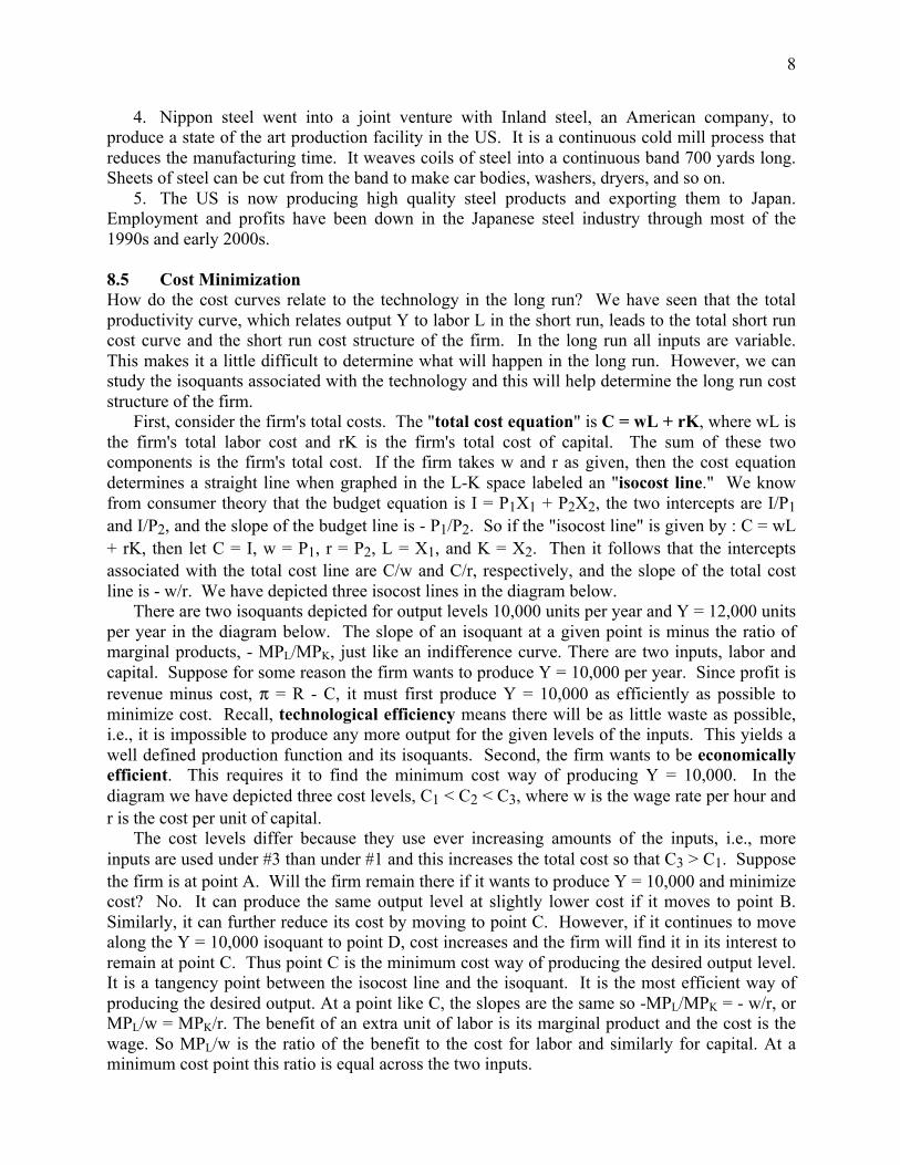
First, consider the firm's total costs. The "total cost equation" is C = wL + rK, where wL is the firm's total labor cost and rK is the firm's total cost of capital. The sum of these two components is the firm's total cost. If the firm takes w and r as given, then the cost equation determines a straight line when graphed in the L-K space labeled an "isocost line." We know from consumer theory that the budget equation is I = P1X1 + P2X2, the two intercepts are I/P1 and I/P2, and the slope of the budget line is - P1/P2. So if the "isocost line" is given by : C = wL + rK, then let C = I, w = P1, r = P2, L = X1, and K = X2. Then it follows that the intercepts associated with the total cost line are C/w and C/r, respectively, and the slope of the total cost line is - w/r. We have depicted three isocost lines in the diagram below.

There are two isoquants depicted for output levels 10,000 units per year and Y = 12,000 units per year in the diagram below. The slope of an isoquant at a given point is minus the ratio of marginal products, - MPL/MPK, just like an indifference curve. There are two inputs, labor and capital. Suppose for some reason the firm wants to produce Y = 10,000 per year. Since profit is revenue minus cost, π = R - C, it must first produce Y = 10,000 as efficiently as possible to minimize cost. Recall, technological efficiency means there will be as little waste as possible, i.e., it is impossible to produce any more output for the given levels of the inputs. This yields a well defined production function and its isoquants. Second, the firm wants to be economically efficient. This requires it to find the minimum cost way of producing Y = 10,000. In the diagram we have depicted three cost levels, C1 < C2 < C3, where w is the wage rate per hour and r is the cost per unit of capital.

The cost levels differ because they use ever increasing amounts of the inputs, i.e., more inputs are used under #3 than under #1 and this increases the total cost so that C3 > C1. Suppose the firm is at point A. Will the firm remain there if it wants to produce Y = 10,000 and minimize cost? No. It can produce the same output level at slightly lower cost if it moves to point B. Similarly, it can further reduce its cost by moving to point C. However, if it continues to move along the Y = 10,000 isoquant to point D, cost increases and the firm will find it in its interest to remain at point C. Thus point C is the minimum cost way of producing the desired output level. It is a tangency point between the isocost line and the isoquant. It is the most efficient way of producing the desired output. At a point like C, the slopes are the same so -MPL/MPK = - w/r, or MPL/w = MPK/r. The benefit of an extra unit of labor is its marginal product and the cost is the wage. So MPL/w is the ratio of the benefit to the cost for labor and similarly for capital. At a minimum cost point this ratio is equal across the two inputs.

9

The long run expansion path depicted above captures the long run adjustment of the firm

holding input prices fixed. As the firm expands its operations it moves from A to B to C along the expansion path. Each point represents a tangency between an isoquant and a cost line so each point is optimal in the sense that the firm maximizes profit and produces its output in a least cost fashion. So each point on the expansion path is technologically efficient, economically efficient, and maximizes profit. It is literally impossible for the firm to pick another point and do better. One way of interpreting this situation is to imagine a new firm that grows and prospers

over time. As the firm expands its operations to meet its demand, it will need more labor and more capital. But it wants to produce as efficiently as it can and the expansion path is the most efficient way. Another way of interpreting the graph is for a firm that is developing a strategy for growth in the future. Perhaps the firm is going to expand into new markets. In order to do so, it must produce more and do so in as efficient a way as possible. So the graph may depict the firm's plans for growing over time.

labor

capital

Y = 10,000

Y = 12,000

••

•

• •

A

B

C

DE

C /w C /w C /w1 2 3

C /r

C /r

C /r1

2

3

labor

capital

Y = 10,000Y = 12,000

••

•••A

B C

C /w C /w C /w1 2 3

C /r

C /r

C /r1

2

3

Y = 14,000

expansion path

10

We can relate total cost to output in the long run in the following way. As the firm increases

its output, it also increases its inputs and hence its cost. It is then the spacing of the isoquants that will determine how fast its total cost increases as output increases. From before, we know that the spacing of the isoquants is determined by the firm's returns-to-scale. If returns-to-scale are constant, the isoquants are evenly spaced. If returns-to-scale are increasing, then the isoquants "bunch up." If returns-to-scale are decreasing, then the isoquants tend to "spread out." This affects total long run cost. When returns-to-scale are constant, total cost increases in the same way as output. The total cost curve will be a straight line. The total cost curve will be "curved" when IRS or DRS prevail. For some technologies, there are ranges for each type. Consider doubling output at each step in the diagram above. (Output doubles from a to b, b to c, and so on. Let Y =1 at a, Y = 2 at b, Y = 4 at c, and Y = 8 at d.) Recall that cost doubles when we double all inputs; cost increases by the same percentage as the inputs. When the isoquants bunch up, as they do in the case of IRS, output increases more than the inputs do (point a). On the other hand, when the isoquants spread out, the case of DRS, output increases slower than the inputs (point d). At point a there is IRS so a doubling of output requires only a small increase in the inputs between a and b. So total cost increases by less than 100%.

Example At point a inputs increase by 20% (less than doubling) while output goes up by 100% (doubles). Total cost increases by only 20% (100%x(12-10)/10). So the TC curve on the right is very flat in range a - b - c. However, eventually DRS set in and it takes a larger increase in the inputs in order to double output. For example, inputs might have to increase by 150% to get output to increase by 100%. So in moving from point c to point d, output increases by 100% from Y=4 to Y=8 while total cost increases by 150% (150% = 100%x(40-16)/16) in going from 16 to 40.

The LRMC and LRAC curves can be derived from the long run TC curve. If the TC curve has the slope depicted above, then the LRMC and LRAC will be U-shaped. The short run AC and MC curves are U-shaped because increasing marginal returns to the variable inputs are eventually followed by diminishing marginal returns. The long run AC and MC curves are U-shaped because IRS is followed eventually by DRS. (If CRS prevails throughout so the firm can simply replicate itself when it scales up its operations, then the isoquants are evenly spaced so points a - d would be evenly spaced and the TC curve would be a straight line, the LRMC and LRAC curves will be horizontal straight lines, and LRMC = LRAC. This is a good "benchmark case to consider.)

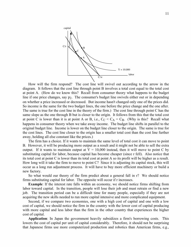
If something in the economic environment changes, the firm must respond and its response will be geared toward minimizing cost and maximizing profit. If w or r change, for example, then the slope of all of the cost lines will change. Suppose the firm is at point A in the diagram above and r falls, as it did in the US from 1990 to 1997 and from 2000 to 2004. Then w/r increases in magnitude and the cost lines become steeper. Graphically, the vertical intercept increases following the arrow and the cost line swivels outward. This is the same response as would happen in consumer theory if P2 fell.

K

L

expansionpath

TC

Y• •

•

•

ab

c

d

• • •ab

d•

1 2 4 8

c161210

40

11

How will the firm respond? The cost line will swivel out according to the arrow in the

diagram. It follows that the cost line through point B involves a total cost equal to the total cost at point A. (How do we know this? Recall from consumer theory what happens to the budget line if one price changes, say p2. The consumer's budget line swivels either out or in depending on whether a price increased or decreased. But income hasn't changed only one of the prices did. So income is the same for the two budget lines, the one before the price change and the one after. The same is true for the cost line in the theory of the firm.) The cost line through point C has the same slope as the one through B but is closer to the origin. It follows from this that the total cost at point C is lower than it is at point A or B, i.e., CC < CA = CB. (Why is this? Recall what happens in consumer theory when we take away income. The budget line shifts in parallel to the original budget line. Income is lower on the budget line closer to the origin. The same is true for the cost lines. The cost line closer to the origin has a smaller total cost than the cost line further away, holding all else constant like the prices.)

The firm has a choice. If it wants to maintain the same level of total cost it can move to point B. However, it will be producing more output as a result and it might not be able to sell the extra output. If it wants to maintain output at Y = 10,000 instead, then it will move to point C by substituting capital for labor, because capital has become cheaper (since r fell). Also notice that its total cost at point C is lower than its total cost at point A so its profit will be higher as a result. How long will it take the firm to move to point C? Since it is adjusting its capital stock, this will occur as a long run adjustment process. It will have to buy more efficient machinery or build a new factory.

So what would our theory of the firm predict about a general fall in r? We should notice firms substituting capital for labor. The opposite will occur if r increases.

Example: If the interest rate falls within an economy, we should notice firms shifting from labor toward capital. In the transition, people will lose their job and must retrain or find a new job. The transition period can be a difficult time for many people, especially if they are not acquiring the new skills needed to run more capital intensive and more complicated equipment.

Second, if we compare two economies, one with a high cost of capital and one with a low cost of capital, we should notice the firm in the country with the lower cost of capital producing with more capital and less labor than the firm in the other country that experiences the higher cost of capital.

Application: In Japan the government heavily subsidizes a firm's borrowing costs. This lowers the cost of capital per unit of capital considerably. Therefore, it should not be surprising that Japanese firms use more computerized production and robotics than American firms, e.g.,

labor

capital

Y = 10,000

• A

C/w

C/r • B

•C

12

compare Toyota and GM. In fact, Japan has a worker shortage in some areas of the economy and this is going to become more severe as their population ages. So we should expect them to shift toward more capital intensive methods of production.3

8.6 Heavy Manufacturing Leontief originated use of an interesting special case based on the following, Y = min(AL, BK), where A and B are constants. There are three cases to consider. First, suppose that AL < BK. Then Y = min(AL, BK) = AL. Second, if AL > BK, then Y = min(AL, BK) = BK. Finally, if AL = BK, then Y = min(AL, BK) = AL = BK. An isoquant is "L-shaped" as depicted below.

Example : Let A = 1/3 and B = 1. Then Y = min(L/3, K) is the production function. To produce Y = 1, 1 machine requires three workers. This is point a in the diagram. More capital

without more labor, point b, will not allow the firm to produce more output. (This is where BK > AL. Why? Because BK = 1x2 = 2 > 1 = (1/3)x3 = AL at point b.) On the other hand, more labor without more machinery, point c, will also not produce more output. (Because AL = (1/3)x6 = 2 > 1x1 = BK at point c.) At point a, AL = (1/3)x3 = 1 = 1 = 1x1 = BK. To increase output, the firm must buy another machine so K = 2 and hire 3 more workers. At point d, AL = (1/3)x6 = 2 = 2 = 1x2 = BK.

The Leontief technology characterizes a production process with no substitution between capital and labor. The two inputs are perfect complements. Some economists believe the Leontief technology is a good description of many manufacturing processes in heavy industry, e.g., Boeing jets, GM cars, Monsanto chemicals.

What would the firm's cost structure look like? In a sense it only has a long run cost structure because it can only increase output by increasing both inputs. And it would appear that constant returns to scale prevails. So the cost structure of the firm will look like the following,

To see this, recall that if L2 = 2L1 and K2 = 2K1, cost doubles, C2 = wL2 + rK2 = w(2L1) +

r(2K1) = 2[wL1 + rK1] = 2c1. However, in this case, if one machine is increased to two machines 3 As an aside, they are even developing the technology to build robots to act as personal servants doing household chores!

K

LY = 1

2

1

3 6

Y = 2

••

••

a

b

c

d

cost

MC = AC

Y

13

and 3 workers is increased to six in order to double the output, then Y2 = 2Y1. It follows that average cost does not change, AC2 = C2/Y2 = 2C1/2Y1 = AC1, i.e., average cost is constant. If the average cost is constant, then the marginal cost must also be constant.

8.7 Scientific Management Circa 1790 in the US, most production was very small scale. Skilled craftsmen had to fashion individual parts and then assemble the parts into a wagon, for example. Most clothing, as another example, was produced at home. Eventually, however, someone figured out that if one could standardize parts, skilled craftsmen would not be needed to assemble the parts. The drive to "standardize" parts for easy assembly began in the manufacture of muskets and later rifles. Typically, a skilled worker would have to file a part down to make it fit. However, as the machine tool industry developed, manufacturers of parts were able to improve the quality of the parts produced. Just prior to the American Civil War, rifle manufacturers had perfected these production techniques. Standardization was then applied to other industries.

Frederick Taylor, a mechanical engineer, sought to standardize all activities taking place in a factory. He was most famous for his time and motion studies. He would break down a production process into different parts and try to make each activity more efficient thus increasing the overall efficiency of the entire production process. For example, he calculated that the optimal weight for a shovel was 21.5 lbs and he designed special shovels of different sizes that could be used to lift 21.5 lbs, whatever the material. He was especially interested in improving the production of steel. Basically, he wanted to apply the concept of standardization to each activity involving production, not just the parts. Each person shoveling coal, for example, would be taught to do so in the same way, the most efficient way as devised by Taylor. He also believed that the productivity of a worker could be carefully measured and that the worker should be compensated accordingly. Workers often resented the introduction of his methods. His ideas were not widely accepted. It was really one of his followers Henry Gantt that popularized Taylor's ideas.

Application: Amazon provides a modern example of this sort of management activity. They closely monitor the activities taking place in their warehouse operations. Their goal is to maximize efficiency and speed. Workers are timed on various activities such as how many orders they can box per minute, how many mistakes they make in a shift, and so on. Breaks from the line and lunches are also carefully monitored.

8.8 "Lean Manufacturing" The traditional method of mass production stemmed from the use of the assembly line and standardized interchangeable parts. The first widespread example of high quality interchangeable parts comes from the manufacture of firearms prior to the Civil War in the 1860's. The technology evolved to the point where parts manufacturers could maintain a certain level of quality. This meant that one rifle barrel, for example, was much like another. One firing pin was much like another. Prior to this, skilled craftsmen had to "file" and "shave" each part so it would fit together with the other parts. Production was very time consuming and labor intensive, especially in skilled labor. However, the technological advances made in the mid 19th century in producing standardized parts meant that it was much easier to put the parts together. This had two implications. First, costs fell as workers became more productive, and much of the lower cost was passed on to consumers in lower prices. Second, skilled craftsmen were no longer needed, at least to put the parts together; practically any worker could put the parts together with a minimum amount of training. This further lowered costs. Eventually, machines were designed

14

that could put the parts together. Skilled people were needed to fix and maintain the machines that made the new standardized parts, however.

This revolution carried over to automobiles and other areas of manufacturing. In the automobile industry, Henry Ford was the first to realize that he could lower the cost of a car if the parts were standardized because he wouldn't need to hire skilled workers and he could build cars faster. As it turned out, he decided to pay his workers a higher wage than the going rate anyway to ensure their loyalty. This idea of mass producing a product through the use of standardized parts and mostly unskilled workers dominated thinking about production for quite a long time. Indeed, Taylor's famous "time and motion" studies were an attempt to design the system of manufacturing so workers would make a minimum amount of movements in doing a particular task.

Edward Demming and his followers had a slightly different theory of production. There were two parts to this alternative theory that were critical. First, at the end of a production run in a traditional "Ford style" factory, there were always some defective cars. Typically, they were shunted off to a separate warehouse and a special work crew had to be brought in usually on the weekend at time and a half pay to fix the defects. It was thought that the quality of the product was produced on the shop floor. Lazy workers or tired workers would produce more defective units than good workers. Demming argued to the contrary that quality was produced in the corporate boardroom, not on the shop floor, because that is where the decisions about how the car is designed and produced are made. For example, at the end of a production run in an auto plant some of the headlights will be put in upside down. Workers have to be brought in on a Saturday to fix the headlights. Demming argued that the headlight should be designed so there is only one way to put it in the car. That way there won't be any defective cars at the end of a shift. This philosophy is known as Total Quality Management (TQM). The TQM philosophy also strongly urges managers to listen to the ideas of their workers because many times they have practical ideas that are useful in doing things more efficiently and this lowers costs. There are other features of TQM you can learn about in your management classes.

The second element has to do with inventories. In the traditional style of manufacturing there is a warehouse of parts and a warehouse of the finished product. When parts are needed, workers have to go to the warehouse to get them. This is very costly and wasteful. With "just-in-time" inventory the parts arrive from the supplier right before they are needed and the company produces exactly the amount the buyer ordered, no more and no less. For example, suppose A supplies B and B supplies C. A ships parts to B "just-in-time" for B to produce its product. B then ships its product to C just when C needs it. In the extreme case, no inventories of parts or the finished product are needed. Of course, this assumes the public infrastructure can handle the various transportation needs of A, B, and C in making their deliveries on time.

There are several problems with this new philosophy. First, it is not always true that all aspects of quality can be thought of beforehand and built into the design of the product to make its assembly completely foolproof. Mistakes and defects will occur.

Second, designs are not always perfect. A design flaw can still occur under TQM that can lead to defective quality. For example, sidesaddle gas tanks in pickup trucks can explode if there is a side impact. As another example, Sony laptop batteries developed an embarrassing propensity for exploding, which led to a major recall. Design flaws can lead to a major recall, which is very costly. There is nothing in TQM that can eliminate them. Keep in mind that it is very costly to weed out design defects before they occur. A firm must compare the costs of reducing design problems with the benefits. Clearly, if the cost of reducing design flaws is greater than the benefit at the margin, it does not pay to eliminate all of them.

15

Third, "just-in-time" inventory assumes that a firm can make and receive deliveries when it needs to. But suppose that all firms want to use the "just-in-time" method. In that case it is entirely possible that the public infrastructure won't be able to handle the traffic flows efficiently and massive congestion may occur. Production at one particular firm may be delayed if its parts are delayed in arriving. Some firms in Tokyo, for example, are starting to keep modest inventories now because snarled and congested traffic has led to delays in their production schedule.

Finally, a labor strike at a supplier can shut down a firm's operations if it has no inventory of parts. This may not be a problem in a country where labor strikes are unheard of. However, in the United States, Canada, and western Europe companies have been shut down because of strikes. Having an inventory of parts allows a firm some flexibility in meeting the needs of its customers even if one of its suppliers experiences a strike.

Application: Sometimes a good idea in one culture doesn't quite translate to another culture. Strikes and work stoppages can cause problems in the supply chain and can spill over from one country to another. This is not much of a problem in Japan, especially when Japanese companies were first applying some of these new ideas in the 1950s and 1960s, but they can become issues in other countries where labor is more powerful.

On April 24, 1997 The New York Times reported that numerous strikes threatened to shut down production of a broad variety of popular cars and trucks made by all three of the domestic auto producers. For example, an engine plant employing 1,856 workers for the Chrysler Company went on strike because the company was going to "outsource" some of the work and re-deploy workers to lower paying tasks. This forced Chrysler to shut down some of its other assembly plants because it didn't have an inventory of engines and it had to lay off 21,000 additional workers. Production of the Jeep Grand Cherokee, the Dodge Ram pickup and van, the Dodge Dakota pickup, and the Dodge Viper were temporarily halted as a result. The profits of the three automakers were down that quarter as a result of the strike. This has continued to be a problem in the 2000s.

Strikes and labor stoppages have caused similar problems in Europe. There have been numerous protests by farmers in France, for example, who do not want their subsidies to end. They literally blockade roads and bridges leading into Paris, and within the city, that bring the city to a complete standstill. In 2005 riots broke out in several poor suburbs of Paris amongst immigrant groups protesting the lack of jobs and opportunity, as well as police brutality. Business ground to a halt as the rioting spread to hundreds of towns all across France. (NPR, Nov 8, 2005)

8.9 Competing With Japan and Europe In 1950 the United States produced half the world's GNP. Half! During World War Two much of our competition was literally blown up. Britain, France, Germany, and Japan all suffered tremendously during the war. For example, Dresden, Germany was targeted by Allied bombers because it was an industrial city suspected of producing war material. Hiroshima and Nagasaki were chosen as targets for the atom bomb because they were industrial cities. Few countries have ever held such a dominant position. The last forty years have seen a gradual shift back to a situation of more even parity across countries. The U.S. is still the world leader but does not have the same sort of dominant position it had in 1950.

During the 1970's U.S. industry was under attack from foreign competition. First, the Japanese started selling inexpensive, some might say cheap, electronics goods like transistor radios, and small cars like the Toyota Corolla, the Honda Civic, and the Datsun. (Essentially, the Honda company took one of their motorcycle engines, built a small car around it, and called it

16

the Civic.) Slowly, Japanese companies began to compete head-to-head with American companies in steel, automobiles, and stereo equipment and televisions. In each of these areas the Japanese became the low cost producer. As such, they could charge a lower price and out-compete American companies. American companies were criticized as having too many managers, not caring about quality but only about how to market a product, and producing slipshod quality. Many steel firms in the U.S. went under. American companies no longer produce stereo equipment for the mass market, televisions, and VCR's, even though the technology was invented in the U.S. Even baseballs are no longer produced in the United States but are produced in China, South Korea, and the Philippines!!! It seemed as if America could do nothing right.

As depicted in the diagram, if the Japanese are more efficient in some industry than the American company, their cost will be lower. They can charge a lower price than the American company can, as indicated, earn a profit, and drive the American company out of business. A good case in point is consumer electronics. Virtually, no American companies are mass producing consumer electronics in the US anymore.4

Throughout the 1990s the Japanese economy was in a deep recession. It began when the land market "price bubble" burst. People were speculating on land and this was driving prices for housing "sky high." At one time the grounds of the emperor's palace were valued at about the same price as all of California, or so they claimed! When the land market disintegrated, the stock market in Japan also collapsed. People lost huge amounts of savings over night. Confidence was lost. And now the Japanese are finding that they must move some of their production facilities to other countries where labor is cheaper.

Since the early 1980's American companies have had to redesign how they do business. They have had to become more efficient and lower their costs. After twenty years of adjusting to competition from abroad, American companies can now compete on an even basis in a broad variety of markets. So the Japanese appear to be going through what the U.S. went through in the 1970's and 1980's. For example, if you buy a Sony VCR, it is more likely to be made in Malaysia than in Japan.

As mentioned above, the steel industry has made a major come back in the U.S. Although, the industry is not what it once was. Jobs are more "skill intensive" than ever before. One must know something about basic mathematics and simple statistics to run a production line in a modern specialty steel company. Having said that, U.S. firms are now exporting highly specialized molded plastic and steel products back to Japan. The irony is that some of those

4 There are a number of smaller companies like Bose, for example, that market high end stereo products.

cost

MC = AC

Y

cost

MC = AC

Y

Japan United States

17

products eventually find their way back to the U.S. as the component of a VCR, car, or video camera, etc.

Europe on the other hand has also suffered from the Japanese competitive onslaught of the 1970's and 1980's but to a much lesser extent because European governments protect their economies more than the U.S. does. However, Britain was trying to deregulate its economy in the 1970's and 1980's under Margaret Thatcher as the U.S. did. So the British were more open to allowing the Japanese to invest in their economy. Several Japanese auto producers, e.g., Toyota, Nissan, built auto assembly plants in Britain. This raises a major problem for other European countries. Is a Toyota Camry, best selling car in the world now, made in Britain a British car or a Japanese car? If it is a British car, then there is no import fee when it is sold in France, for example. If it is a Japanese car, then there will be an import fee if it is sold in France. So Europeans are a bit wary of allowing the Japanese into their market. To get around import duties American companies have subsidiaries in Europe. For example, GM is the second largest seller of cars in Europe right behind Volkswagon throughout the 1980s and 1990s. However, this doesn't help American workers.

The second main issue facing Europe is its social welfare policies. Most countries in Europe, the exception being Britain, have much larger unemployment compensation programs, food stamp, and assistance programs, housing subsidies, and the like. All of these programs require taxes to fund them and these taxes are born by both sides of the market but tend to raise prices by raising cost. However, this means that European countries will have difficult competing with other countries like the U.S. or Japan that do not have such extensive welfare assistance programs. Unemployment is much higher in Europe as well. As of May, 1998 unemployment was running at about 4.5% in the U.S. and two or three times that in Europe depending on the country. Business also has to cope with more regulation in France, the Netherlands, Italy, and so on. Regulations can be very costly to comply with.

The point is that anything that raises cost makes it harder for a company to compete. Taxes, regulations, import and export duties all raise cost. Protecting an industry, as is done in Europe, can lead to the industry becoming inefficient over time. In this sense Europe is worried that it will be unable to compete against Japanese and American companies.

It is interesting to note that in the 1980s everyone was talking about emulating the Japanese, who were out-competing America and Europe. In 2001, there are people in Japan saying they need to "Americanize" their economy to become more competitive. And, just as American students started shifting away from engineering and science toward business degrees since the early 1980s, the same phenomenon is happening in Japan.5

Since 2005 the competition is coming from China. Many products that used to be made in the U.S. or Europe are now made in China. And they are starting to compete with Japan as well. One exception to this appears to be Dell Computers in the U.S. No other major computer manufacturer makes computers in the U.S. In fact, I.B.M., which created the PC market in 1981 and is Dell's last U.S. rival, is quitting. It announced in 2004 that it is selling its PC unit to Lenovo, the large Chinese computer company.

"It's been a long time since one of our competitors actually made a computer," said Michael S. Dell. Dell has three large assembly plants in the United States, and the company recently announced in 2004 that it would build a fourth plant, twice as big as the others, near Winston-Salem, N.C. Dell's decision to expand its plants in the U.S. is based solely on cost consideration; it is simply more efficient to produce computer equipment closer to the market.

5 NYTimes, May 17, 2008

18

8.10 Business financing Businesses actively use the credit markets to finance their operations and smooth the flow of the revenue against their cost. For example, many businesses in the US gear up for the Christmas shopping season in the late summer and early fall. They borrow from banks and other financial intermediaries to hire extra labor, equipment, and raw materials. Then when the extra output is sold at Christmas the additional revenue is used to pay off the amount borrowed earlier.

As another example, car manufacturers gear up production of the new models well in advance of selling them in the fall. They can borrow in order to provide easy credit to dealers to get the old models off the lot in order to get ready for the new models. Then they can repay the loans from the revenue flow from the new models when they are sold.

Consider a simple two period example. Let Π1 be profit in period 1, R1 be revenue in period 1, C1 be cost in period 1, Π 2 be profit in period 2, R2 be revenue in period 2, and C2 be cost in period 2. If the credit market is not used then we have

Π1 = R1 - C1, and

Π2 = R2 - C2. In equilibrium economic profits are zero so R1 = C1 and R2 = C2, i.e., costs incurred in a

given period must be covered by revenue in that period. If R1 is low for some reason, then the firm has to cut back production to lower cost C1. If R2 is expected to be high, output can expand which raises C2. However, the firm can improve its efficiency by borrowing when revenue is low and repaying when revenue is high. Let B be the amount borrowed in the first period. Then we have instead,

R1 + B = C1, and

R2 - B(1+r) = C2. This allows the firm to maintain output and cost C1 and C2. R1 can be low without affecting

production and cost decisions since the firm can borrow from the credit markets. An extreme case is where the firm has to borrow to get its operation up and running. In that

case R1 = 0 and B = C1, and borrowing covers cost. New firms provide plenty of examples. Amazon.com is a good case in point. It borrowed to get its web site going and then endured several years of negative profits, borrowing from investors and the credit markets. Eventually, however, they were able to turn a profit and repay some of the loans.

During the massive credit crunch of 2008, debt financing was completely unavailable. Credit markets were frozen; no one was lending. If a firm cannot borrow to smooth its cash flow, then if revenue is low, its cost must be low in the short run. The main way to lower cost in the short run is by reducing the variable inputs and the main variable input is labor. Large layoffs became inevitable and this exacerbated the downturn.

8.13 Uncertainty The future is uncertain but firms have to make decisions now. How that uncertainty is resolved matters to the firm's decision making now. For example, suppose the firm thinks the demand for its products will increase in the near future. If the firm invests in plant and equipment now and dramatically expands its production capacity now, serious problems could arise if the expected increase doesn't occur.

Imagine a setting where there is a firm that must decide whether to expand its facilities or not by building more factory space and equipping it. The future is uncertain though; demand could be high, or it could be low. Suppose the firm places the probability of its being high at q and its

19

being low at 1 - q. The probability q is a small positive number less than one and since we are assuming there are only two events, high demand or low demand, the probabilities must sum to one, or 100%, so the probability of demand being low is 1 - q. So q + (1 – q) = 1 = 100%. For example, suppose q = 1/4. That means the firm thinks there is a 25% chance its demand will be high in the future. In that case, there is a 75% chance of its being low. So q = 1/4 = 25% and 1 - q = 3/4 = 75%.

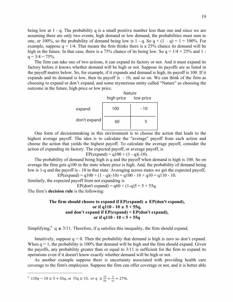
The firm can take one of two actions, it can expand its factory or not. And it must expand its factory before it knows whether demand will be high or not. Suppose its payoffs are as listed in the payoff matrix below. So, for example, if it expands and demand is high, its payoff is 100. If it expands and its demand is low, then its payoff is - 10, and so on. We can think of the firm as choosing to expand or don’t expand, and some mysterious entity called “Nature” as choosing the outcome in the future, high price or low price.

One form of decisionmaking in this environment is to choose the action that leads to the

highest average payoff. The idea is to calculate the "average" payoff from each action and choose the action that yields the highest payoff. To calculate the average payoff, consider the action of expanding its factory. The expected payoff, or average payoff, is

EP(expand) = q100 + (1 - q)(-10). The probability of demand being high is q and the payoff when demand is high is 100. So on

average the firm gets q100 in the state where price is high. And, the probability of demand being low is 1-q and the payoff is - 10 in that state. Averaging across states we get the expected payoff,

EP(expand) = q100 + (1 - q)(-10) = q100 - 10 + q10 = q110 - 10. Similarly, the expected payoff from not expanding is

EP(don't expand) = q60 + (1-q)5 = 5 + 55q. The firm’s decision rule is the following:

The firm should choose to expand if EP(expand) EP(don't expand), or if q110 - 10 5 + 55q,

and don’t expand if EP(expand) < EP(don't expand), or if q110 - 10 < 5 + 55q

Simplifying,6 q 3/11. Therefore, if q satisfies this inequality, the firm should expand.

Intuitively, suppose q = 0. Then the probability that demand is high is zero so don’t expand. When q = 1, the probability is 100% that demand will be high and the firm should expand. Given the payoffs, any probability greater than or equal to 3/11 is sufficient for the firm to expand its operations even if it doesn't know exactly whether demand will be high or not.

As another example suppose there is uncertainty associated with providing health care coverage to the firm's employees. Suppose the firm can offer coverage or not, and it is better able 6 110𝑞 − 10 ≥ 5 + 55𝑞, or 55q ≥ 15, 𝑜𝑟  𝑞   ≥ !"

!!= !

!!= 27%.

Naturehigh price low price

expand

don’t expand

100 - 10

60 5

20

to attract high quality workers if it offers the insurance. However, obviously, the insurance is costly and the cost might be high or low. Suppose the cost can be high with probability q, or low with probability 1- q. Suppose the payoffs are as in the table. Calculate the expected payoffs to obtain,

EP(insurance) = q(-50) + (1-q)100 = 100 - 150q EP(no insurance) = q10 + (1-q)60 = 60 - 50q.

The decision rule is: If 100 - 150q 60 - 50q, then offer the insurance. Simplifying, if 0.4 q, offer the insurance.

As another example consider a firm that is thinking about opening a new hotel in another country. Its actions are to open or not to open the hotel and the two states are that its labor costs will be high or low. The payoffs are listed in the table.

The expected payoffs are EP(open) = q50 + (1-q)(-25) = q75 - 25, EP(don't open) = q0 + (1-q)0 = 0.

The decision rule is: If q75 - 25 0, or q 1/3, open the hotel. How does the firm know q? If the firm is contemplating expanding its factory, it can do a

market study to calculate the probability that demand in the future will be high and what the payoffs will be. If the firm is contemplating opening a hotel in another country it can do a study on the demand for travel to that country, and the labor costs in that country. That will help it figure out the probability and the payoffs of its actions. 8.13 Conclusion In this chapter we related the technology to the firm's cost and derived its short run and long run cost structures. In the short run some decisions are fixed and cannot be changed. As we vary the variable inputs like labor in the short run we trace out the productivity of those inputs. When we multiply the use of the input by its unit cost, e.g., wage rate per hour, we obtain the short run variable cost curve. This allows us to derive the average and marginal cost curves in the short run. If returns to the variable inputs are first increasing and then diminishing, then the average and marginal cost curves are "U-shaped."

We also derived the long run cost structure. this depends on the returns to scale concept because the firm can basically decide how large it wants to be in the long run. If returns to scale

Nature

insure

don’t insure

high cost low cost

- 50 100

10 60

Naturehigh cost low cost

open

don’t open

50 - 25

0 0

21

are constant, then the long run average and marginal cost curves are horizontal. If returns are increasing, long run average and marginal costs are falling. They are rising if returns to scale are decreasing. We applied the model to competition with other countries, especially Japan, the US auto industry, heavy manufacturing, and discussed the so-called theory of "lean manufacturing."

Important Concepts Short run costs variable cost fixed cost Long run costs U-shaped cost curves Cost minimization Heavy manufacturing costs Lean manufacturing L-shaped LRAC curve Review Questions

1. What is the distinction between fixed and variable costs? Why are some costs fixed?

2. What determines the shape of the total cost curve? 3. Why are the short run cost curves of the firm "U-shaped?" 4. How do the long run cost curves differ from the short run cost curves? 5. What is the relationship between the long run and short run cost structures? 6. Explain how the firm minimizes cost. 7. What is "lean manufacturing?" What are some of the problems associated with

lean manufacturing? Practice Questions 1. Suppose a firm has no fixed costs. Then its short run cost structure is the same as its long

run cost structure. a. True. b. False.

2. Marginal cost is always equal to average cost under constant returns to scale. a. True. b. False. 3. The long run cost structure in the auto industry is U-shaped. a. Yes. b. No. 4. Let Y = number of college degrees granted, L = faculty, K = classroom space, N =

number of incoming fresh-people, and assume that Y = F(L, K, N). In the short run what would happen to cost if WSU tried to dramatically increase the number of students attending WSU without hiring new faculty or providing any new classroom space?

a. Average Cost would fall if there were diminishing marginal returns. b. Average Cost would rise if there were diminishing marginal returns. c. Average Cost would fall if there were decreasing returns to scale. d. Average Cost would rise if there were decreasing returns to scale.

22

5. From the previous question, if we double the usage of classroom space, double the

number of faculty at WSU, and double the size of the incoming class of students, but only increase the number of degrees granted by 25%, what must be true of cost?

a. Average Cost would fall if there were diminishing marginal returns. b. Average Cost would rise if there were diminishing marginal returns. c. Average Cost would fall if there were decreasing returns to scale. d. Average Cost would rise if there were decreasing returns to scale.

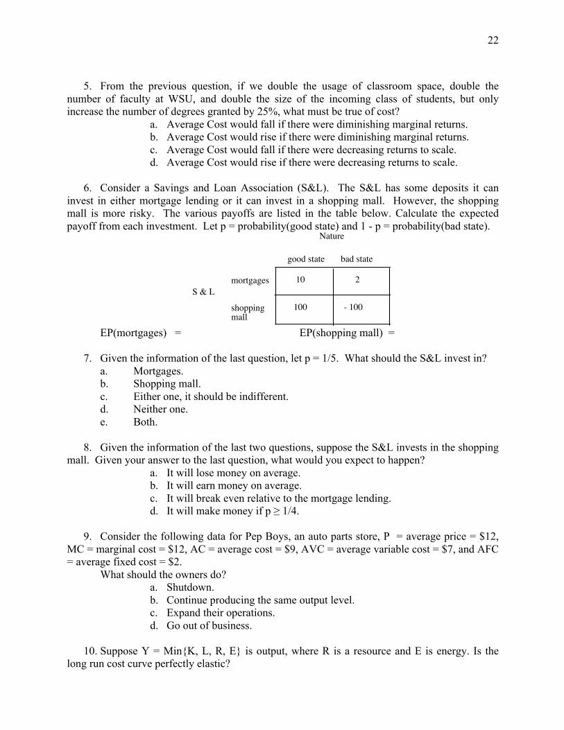
6. Consider a Savings and Loan Association (S&L). The S&L has some deposits it can

invest in either mortgage lending or it can invest in a shopping mall. However, the shopping mall is more risky. The various payoffs are listed in the table below. Calculate the expected payoff from each investment. Let p = probability(good state) and 1 - p = probability(bad state).

Nature

S & L

good state bad state

mortgages

shopping mall

10 2

100 - 100

EP(mortgages) = EP(shopping mall) = 7. Given the information of the last question, let p = 1/5. What should the S&L invest in? a. Mortgages. b. Shopping mall. c. Either one, it should be indifferent. d. Neither one. e. Both. 8. Given the information of the last two questions, suppose the S&L invests in the shopping

mall. Given your answer to the last question, what would you expect to happen? a. It will lose money on average. b. It will earn money on average. c. It will break even relative to the mortgage lending. d. It will make money if p ≥ 1/4.

9. Consider the following data for Pep Boys, an auto parts store, P = average price = $12,

MC = marginal cost = $12, AC = average cost = $9, AVC = average variable cost = $7, and AFC = average fixed cost = $2.

What should the owners do? a. Shutdown. b. Continue producing the same output level. c. Expand their operations. d. Go out of business.

10. Suppose Y = Min{K, L, R, E} is output, where R is a resource and E is energy. Is the long run cost curve perfectly elastic?

23

Answers 1. a. 2. b, They are not equal in the short run. 3. a. 4. b. 5. d. 6. 2 + 8p and 200p - 100 7. 2 + 8/5 and – 60 so a is the answer. 8. It will lose money on average. 9. p < Ac so the firm is losing money but p > AVC so it should continue to produce. 10. Yes, the extra inputs will not change this result of CRS in the long run.