8. Representing displacements - Computer...

8. Representing displacementsMechanics of Manipulation

Matt [email protected]

http://www.cs.cmu.edu/~mason

Carnegie Mellon

Lecture 8. Mechanics of Manipulation – p.1

Lecture 8. Representing displacements.

Chapter 1 Manipulation 1

1.1 Case 1: Manipulation by a human 1

1.2 Case 2: An automated assembly system 3

1.3 Issues in manipulation 5

1.4 A taxonomy of manipulation techniques 7

1.5 Bibliographic notes 8

Exercises 8

Chapter 2 Kinematics 11

2.1 Preliminaries 11

2.2 Planar kinematics 15

2.3 Spherical kinematics 20

2.4 Spatial kinematics 22

2.5 Kinematic constraint 25

2.6 Kinematic mechanisms 34


Exercises 37

Chapter 3 Kinematic Representation 41

3.1 Representation of spatial rotations 41

3.2 Representation of spatial displacements 58

3.3 Kinematic constraints 68


Exercises 72

Chapter 4 Kinematic Manipulation 77

4.1 Path planning 77

4.2 Path planning for nonholonomic systems 84

4.3 Kinematic models of contact 86


Exercises 88

Chapter 5 Rigid Body Statics 93

5.1 Forces acting on rigid bodies 93

5.2 Polyhedral convex cones 99

5.3 Contact wrenches and wrench cones 102

5.4 Cones in velocity twist space 104

5.5 The oriented plane 105

5.6 Instantaneous centers and Reuleaux’s method 109

5.7 Line of force; moment labeling 110

5.8 Force dual 112

5.9 Summary 117


Exercises 118

Chapter 6 Friction 121

6.1 Coulomb’s Law 121

6.2 Single degree-of-freedom problems 123

6.3 Planar single contact problems 126

6.4 Graphical representation of friction cones 127

6.5 Static equilibrium problems 128

6.6 Planar sliding 130


Exercises 139

Chapter 7 Quasistatic Manipulation 143

7.1 Grasping and fixturing 143

7.2 Pushing 147

7.3 Stable pushing 153

7.4 Parts orienting 162

7.5 Assembly 168


Exercises 175

Chapter 8 Dynamics 181

8.1 Newton’s laws 181

8.2 A particle in three dimensions 181

8.3 Moment of force; moment of momentum 183

8.4 Dynamics of a system of particles 184

8.5 Rigid body dynamics 186

8.6 The angular inertia matrix 189

8.7 Motion of a freely rotating body 195


8.9 Graphical methods for the plane 203

8.10 Planar multiple-contact problems 205


Exercises 208

Chapter 9 Impact 211

9.1 A particle 211

9.2 Rigid body impact 217


Exercises 223

Chapter 10 Dynamic Manipulation 225

10.1 Quasidynamic manipulation 225

10.2 Brie� y dynamic manipulation 229

10.3 Continuously dynamic manipulation 230


Exercises 235

Appendix A Infinity 237


Outline.

• Review of spatial displacements

• Homogeneous coordinates

• Plücker coordinates of a line

• Screw coordinates


Review of spatial displacements

Definition: rigid motion

Theorem 2.2: any displacement of En can be represented as arotation composed with a translation.

Definition: a screw is a line plus a pitch.

Definition: a twist is a motion along a screw.

Theorem 2.7 (Chasles’s theorem): every displacement of E3 is atwist.

These can guide design of representations.


Homogeneous coordinates

Recall theorem 2.2: a displacement can be decomposed into arotation followed by a translation.

x′ = Rx + d

We can write it more compactly. Add a fourth component to points:

x =

x1

x2

x3

1

(Remember, we did this before. If the fourth element is 0 we get points

at infinity. Now we’re focusing on ordinary points.)


Transforms using homogeneous coords

Define the homogeneous coordinate transform matrix T :

T =

R d

0 0 0 1

And writex′ = Tx

It’s just a more compact way of writing:

x′ = Rx + d

Especially useful for expressions such as x′ = T3T2T1x.


Plücker coordinates

Screw coordinates are built on top ofPlücker coordinates, which are a wayof representing lines.

Let p be a point on the line;

Let q be the direction vector ;

Let q0 = p × q, the moment vector ;

Then (q, q0) gives the six Plücker co-ordinates ;

(Note choice of p doesn’t matter:

p′ × q = p × q + (p′ − p) × q

= p × q

l

O p

qq0 p q


Plücker’s excess numbers

Plücker coordinates give six numbers. A line requires only four.

First, since q0 = p × q, there is a constraint:

q · q0 = 0

Second, scaling gives same the line

(q, q0) ≡ k(q, q0)

(So, why not normalize, scaling by 1/|q|? Sometimes, as we shallsee, |q| = 0!)


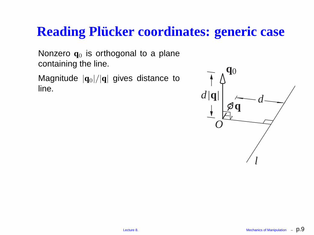
Reading Plücker coordinates: generic case

Nonzero q0 is orthogonal to a planecontaining the line.

Magnitude |q0|/|q| gives distance toline.

q

q0

d

l

O

d q


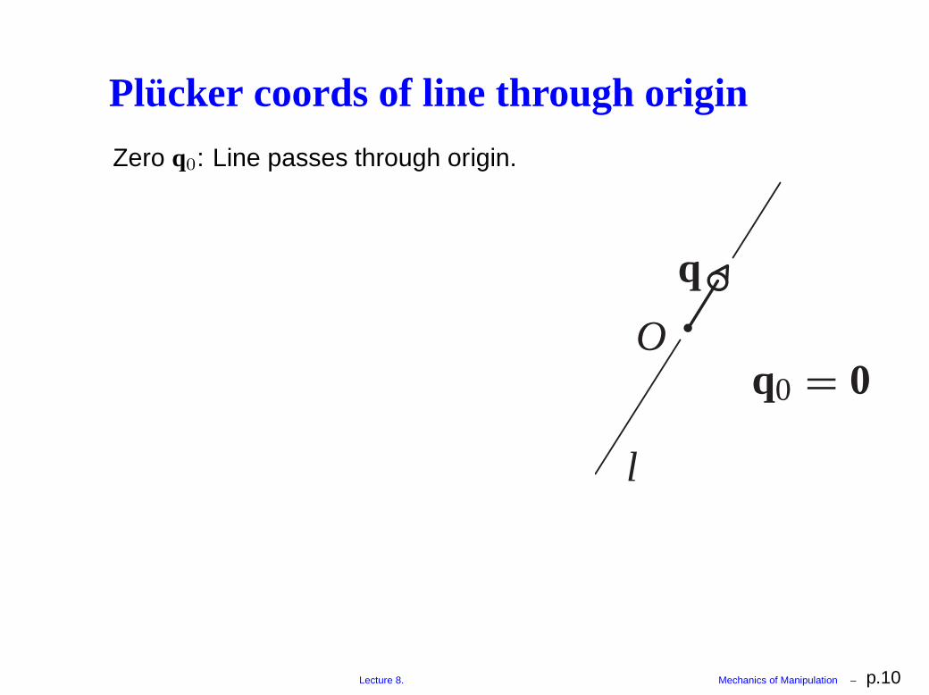
Plücker coords of line through origin

Zero q0: Line passes through origin.

O

l

q

q0 0


Plücker coords of line at infinity

Nonzero q0 is orthogonal to a planecontaining the line.

Magnitude of |q0|/|q| gives distance toline.

Work it out as a limiting process. Holdq0 constant as line goes to infinity.

0

l

q0

q 0

q0

q

l

d


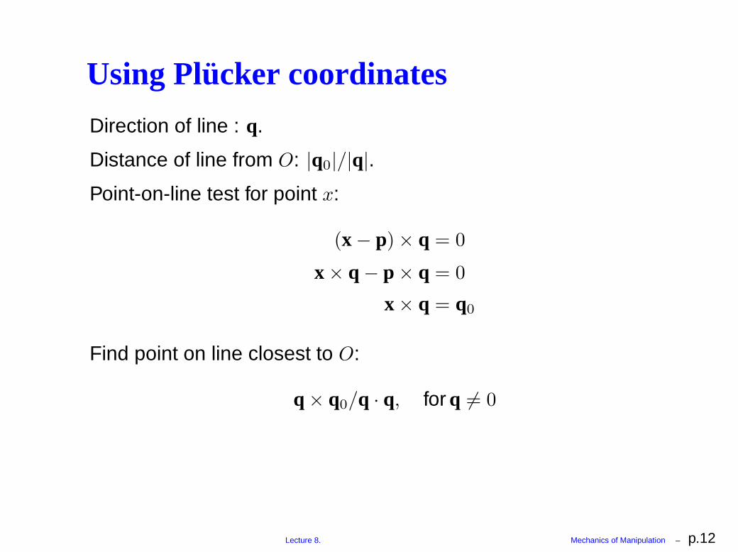
Using Plücker coordinates

Direction of line : q.

Distance of line from O: |q0|/|q|.

Point-on-line test for point x:

(x − p) × q = 0

x × q − p × q = 0

x × q = q0

Find point on line closest to O:

q × q0/q · q, for q 6= 0


A topical example.


Moment about a point

Moment of a line l2 about a point p1.In analogy with unit force in directionq2. What would the torque be?

(p2 − p1) ×

(

q2

|q2|

)

p2 × q2 − p1 × q2

|q2|

q02 − p1 × q2

|q2|


Moment about a line

Moment of a line l2 about a line l1.

Think of the torque at p1, and take thecomponent in the q1 direction:

q1

|q1|·

q02 − p1 × q2

|q2|

q1 · q02 − q1 · p1 × q2

|q1q2|

q1 · q02 + q2 · p1 × q1

|q1q2|

q1 · q02 + q2 · q01

|q1q2|

It’s symmetric. Moment of l1 about l2= moment of l2 about l1.

This interesting product has LOTS ofuses . . . Lecture 8. Mechanics of Manipulation – p.15

Reciprocal product / virtual product

Define reciprocal product , or virtual product :

(q1, q01) ∗ (q2, q02) = q1 · q02 + q2 · q01

For normalized Plücker coordinates, reciprocal product givesmoment between the two lines.


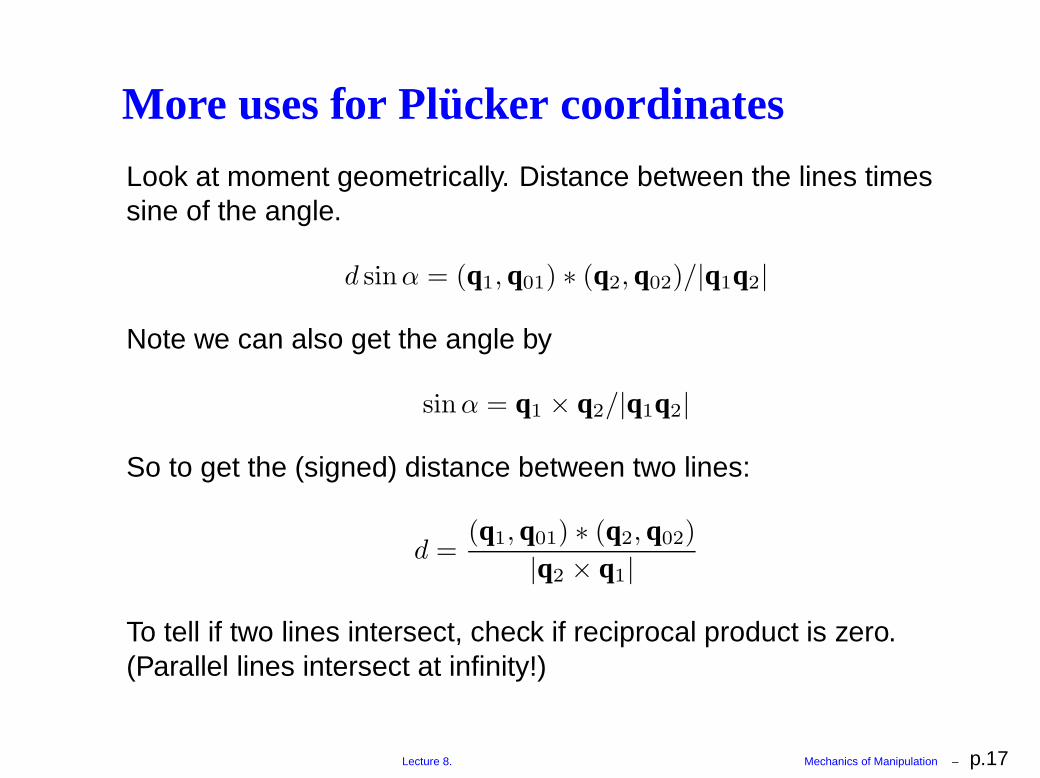
More uses for Plücker coordinates

Look at moment geometrically. Distance between the lines timessine of the angle.

d sinα = (q1, q01) ∗ (q2, q02)/|q1q2|

Note we can also get the angle by

sinα = q1 × q2/|q1q2|

So to get the (signed) distance between two lines:

d =(q1, q01) ∗ (q2, q02)

|q2 × q1|

To tell if two lines intersect, check if reciprocal product is zero.(Parallel lines intersect at infinity!)


Example: using Plücker

Find the angle and distance between the two lines:

l1

l2

x

y

z


Screw coordinates

A screw is a line plus a scalar pitch. Seven numbers?

No! We aren’t really using those six numbers. Plenty of room tosneak pitch in.

Given a line (q, q0), and pitch p. Define the screw coordinates to be(s, s0), where

s = q

s0 = q0 + pq

Why does this work? Recall q · q0 is zero.

To get the pitch back

s · s0 =q · q0 + pq · q

p =s · s0s · s


Special case screws

Zero pitch: just like Plücker coordinates.

Infinite pitch: s = 0.


Representing a twist

A twist is a screw plus a magnitude. Seven numbers?

No! Remember Plücker coordinates don’t use scale. So take Plückercoordinates, normalize them, and scale.

Let θ be the angle of rotation, d the distance of translation, bothnonzero.

Let p = d/θ be the pitch.

(

θs|s|

, θs0|s|

)

Substituting the definition of screw coordinates, we obtain

(

θs|s|

, θs0|s|

)

=1

|q|(θq, θq0 + θpq)

=1

|q|(θq, θq0 + dq)


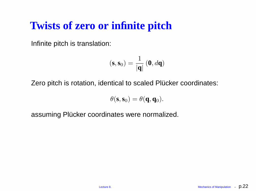
Twists of zero or infinite pitch

Infinite pitch is translation:

(s, s0) =1

|q|(0, dq)

Zero pitch is rotation, identical to scaled Plücker coordinates:

θ(s, s0) = θ(q, q0).

assuming Plücker coordinates were normalized.


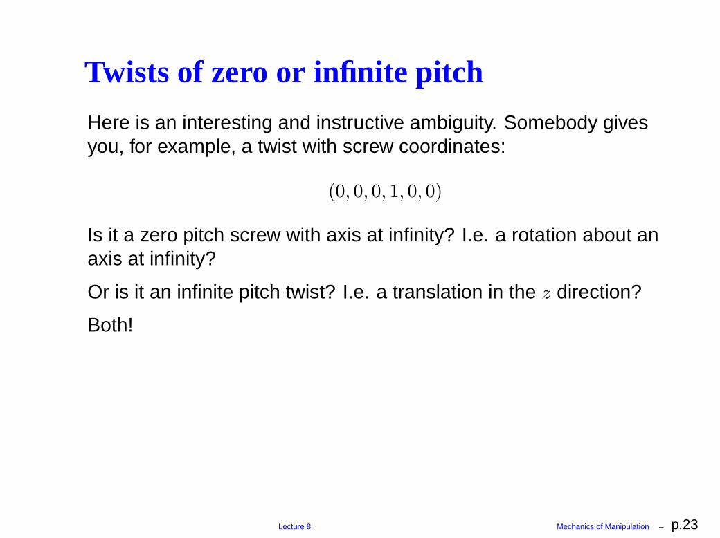
Twists of zero or infinite pitch

Here is an interesting and instructive ambiguity. Somebody givesyou, for example, a twist with screw coordinates:

(0, 0, 0, 1, 0, 0)

Is it a zero pitch screw with axis at infinity? I.e. a rotation about anaxis at infinity?

Or is it an infinite pitch twist? I.e. a translation in the z direction?

Both!


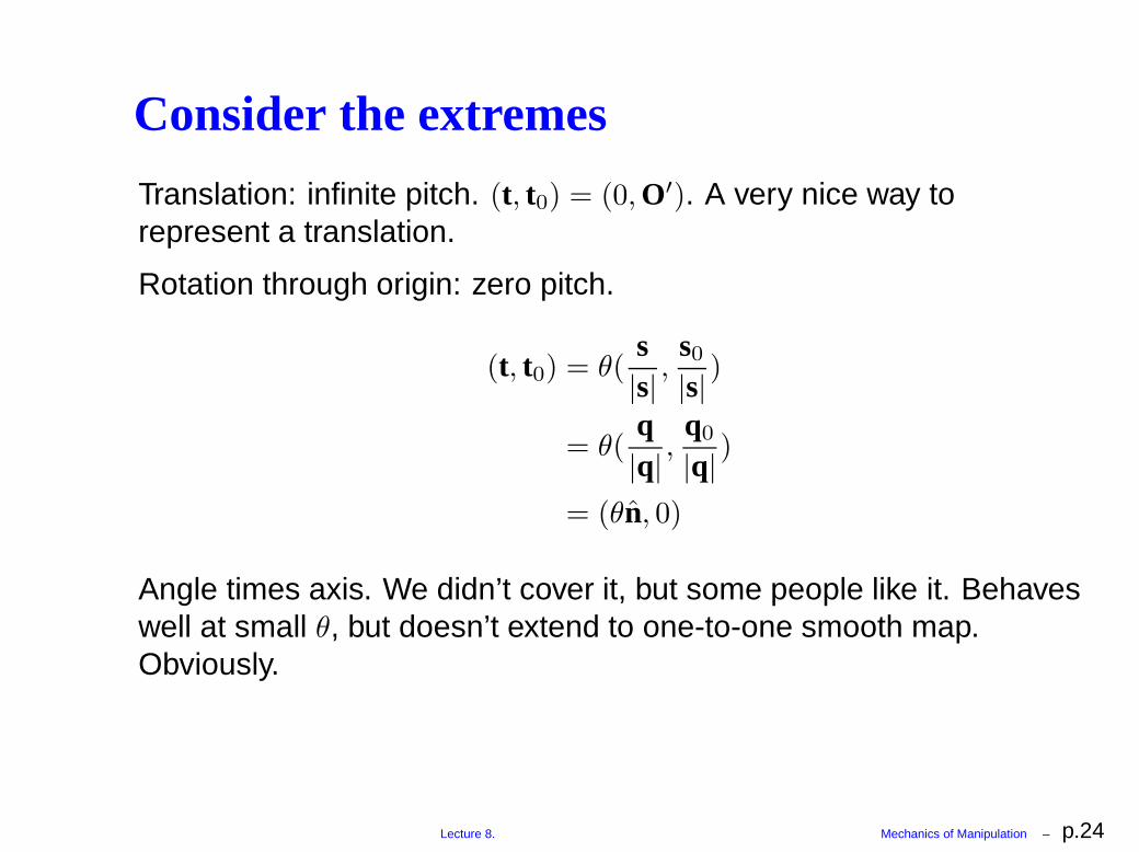
Consider the extremes

Translation: infinite pitch. (t, t0) = (0, O′). A very nice way torepresent a translation.

Rotation through origin: zero pitch.

(t, t0) = θ(s|s|

,s0|s|

)

= θ(q|q|

,q0

|q|)

= (θn̂, 0)

Angle times axis. We didn’t cover it, but some people like it. Behaveswell at small θ, but doesn’t extend to one-to-one smooth map.Obviously.


Differential twists

Consider velocity v along l and angular velocity ωabout l.

Let p be any point on l.

Plücker coordinates of l are

(q, q0) = (ω, p × ω)

Pitch is |v|/|ω| so screw coordinates are

(s, s0) = (ω, p × ω +|v||ω|

ω)

(s, s0) = (ω, p × ω + v)

v

p

l

vv0

Op


Differential twists

The vector s0 gives vel of origin v0

(s, s0) = (ω, v0)

So, for differential twists, screw coords are close tostandard practice.

Important corollary. Screw coordinates for differ-ential twists form a vector space. We can add dif-ferential twist screw coordinates, and we can mul-tiply them by scalars.

v

p

l

vv0

Op


Next: Representing constraints.

Chapter 1 Manipulation 1

1.1 Case 1: Manipulation by a human 1

1.2 Case 2: An automated assembly system 3

1.3 Issues in manipulation 5

1.4 A taxonomy of manipulation techniques 7


Exercises 8

Chapter 2 Kinematics 11

2.1 Preliminaries 11

2.2 Planar kinematics 15

2.3 Spherical kinematics 20

2.4 Spatial kinematics 22

2.5 Kinematic constraint 25

2.6 Kinematic mechanisms 34


Exercises 37

Chapter 3 Kinematic Representation 41

3.1 Representation of spatial rotations 41

3.2 Representation of spatial displacements 58

3.3 Kinematic constraints 68


Exercises 72

Chapter 4 Kinematic Manipulation 77

4.1 Path planning 77

4.2 Path planning for nonholonomic systems 84

4.3 Kinematic models of contact 86


Exercises 88

Chapter 5 Rigid Body Statics 93

5.1 Forces acting on rigid bodies 93

5.2 Polyhedral convex cones 99

5.3 Contact wrenches and wrench cones 102

5.4 Cones in velocity twist space 104

5.5 The oriented plane 105

5.6 Instantaneous centers and Reuleaux’s method 109

5.7 Line of force; moment labeling 110

5.8 Force dual 112

5.9 Summary 117


Exercises 118

Chapter 6 Friction 121

6.1 Coulomb’s Law 121

6.2 Single degree-of-freedom problems 123


6.4 Graphical representation of friction cones 127

6.5 Static equilibrium problems 128

6.6 Planar sliding 130


Exercises 139

Chapter 7 Quasistatic Manipulation 143

7.1 Grasping and fixturing 143

7.2 Pushing 147

7.3 Stable pushing 153

7.4 Parts orienting 162

7.5 Assembly 168


Exercises 175

Chapter 8 Dynamics 181

8.1 Newton’s laws 181

8.2 A particle in three dimensions 181

8.3 Moment of force; moment of momentum 183

8.4 Dynamics of a system of particles 184

8.5 Rigid body dynamics 186

8.6 The angular inertia matrix 189

8.7 Motion of a freely rotating body 195


8.9 Graphical methods for the plane 203

8.10 Planar multiple-contact problems 205


Exercises 208

Chapter 9 Impact 211

9.1 A particle 211

9.2 Rigid body impact 217


Exercises 223

Chapter 10 Dynamic Manipulation 225

10.1 Quasidynamic manipulation 225

10.2 Brie� y dynamic manipulation 229

10.3 Continuously dynamic manipulation 230


Exercises 235

Appendix A Infinity 237


8. Representing displacements - Computer...

Documents

Transcript of 8. Representing displacements - Computer...