8 HOUSEHOLD LEVEL FOOD SECURITY AND VULNERABILITY

197

8. INTRODUCTIONIn this section of the assessment, the focus is on the impact of rising food prices on household level food security in Tanzania. There has been widespread concern regarding the surge in staple food prices over the last few years and biofuel developments have been widely recognized, although to a varying degree, as one of the key drivers of the recent price surge and increased price volatility. In this context first generation bioenergy developments represent an additional source of demand for crop production which can lead to price increases, unless followed by adequate supply response.

Furthermore, domestic changes in food prices derive from international and domestic supply and demand shocks which include additional biofuel demand. In fact, it is important to realize that, while there may have been no significant bioenergy developments within the country to date, the globally biofuel mandates have been gaining steam. Therefore, although a domestic bioenergy sector might not yet exist, international policy decisions impact domestic prices which will in turn have an effect on national household food security. Consequently, although developing a domestic biofuel sector is a medium-term plan, households in the short term can still suffer food security impacts due to the changes in prices of the key food staples which are a result of both international and national policies.

Price increase can have a positive or negative impact on countries depending whether they are net food importers or net food exporters. Seemingly, at the household level, price increases are negative for net food consuming households (net-buyers), but positive for net food producing households (net-sellers). The degree to which households will, overall, be made worse or better off depends on the net welfare impact which is based on their overall net position as defined above.

As a concluding remark, it is important to stress that the price changes to which the households are subject are the result of domestic and international supply and demand shocks. Nevertheless, what matters for the households are the domestic price increases. The actual variation in domestic prices will depend on the nature of the commodity being considered, namely if the commodity is a tradable or non-tradable commodity, and therefore on the degree to which international price changes will transmit through

C H A P T E R 8 HOUSEHOLD LEVEL FOOD SECURITY AND VULNERABILITYIr ini Maltsoglou and David Dawe

198

]B

IO

EN

ER

GY

A

ND

F

OO

D

SE

CU

RI

TY

[

to domestic markets. This heavily depends on what domestic trade policies are in place and on exchange rate fluctuations. The degree of transmission is commodity and country specific.

From a policy perspective, it is necessary to understand how these price changes can impact, firstly, the country as a whole and, secondly, household level food security. This will allow the assessment of which price movements to which the country is most vulnerable and which segments, amongst the poor, are most at risk.

A real case scenario should help explain this issue further. Tanzania, for example, has banned the use of maize for ethanol production because it is a key food staple. Nevertheless, due to international biofuel developments, the price of maize has been increasing. This part of the analysis will shed light on the impacts of the resulting increase in the key food staples on different household groups and help identify the vulnerable groups in the country.

The analysis is made up of three main components, namely country level impacts, domestic price movements and household level impacts. At first the focus is on country level impacts in order to understand which price movements to which the country as a whole is most vulnerable. This is done by an assessment on what level domestic price movements are linked to international price movements and a calculation of the price increases in domestic food prices. Thirdly, we focus on household level food security impacts by assessing the impact of increases in food prices on households’ welfare. The key crops for the analysis are identified based on their calorie contribution. As maize and cassava are the two most important food crops, the second and third steps of the analysis mostly focus on these two crops.

In order to run the household level analysis a detailed Household Income and Expenditure Survey (HIES) is needed. In the case of Tanzania this dataset is called the Household Budget Survey (HBS). This dataset could not be used as unfortunately agriculture income is not reported by crop. For this reason a regional dataset collected by REPOA, FAO and the World Bank between 2003 and 2004 was used. This dataset only covers rural households from two regions in Tanzania and therefore policy conclusions at the country level cannot be drawn. Nevertheless, the analysis run with this dataset can illustrate the logic behind the analysis and the kind of policy messages that can be drawn from this assessment component.

Following the introduction, Section 2 ranks the food commodities and outlines the net trade position of the country based on the food security list. Section 3 looks at domestic price trends for the two most important food crops, namely maize and cassava. Section 4 provides an overview of the methodology applied for the household level assessment. Section 5 presents the household level welfare impacts and Section 6 concludes.

199

HOUSEHOLD LEVEL FOOD SECURITY AND VULNERABILITY

8.1 FOOD SECURITY IN TANZANIAThe food security analysis presented here focuses on the main food security crops in Tanzania. The list of food security crops is selected based on their calorie contribution as previously discussed (Table 2.1). The relevant list is included here for ease of reference (Table 8.1).

Based on the per capita calorie ranking previously discussed, the most important food crops in Tanzania are maize, cassava and rice. Maize contributes 33.4 percent of calories, cassava accounts for 15.2 percent of calorie intake and rice provides 7.9 percent of the calories.

T a b l e 8 . 1

Calorie contribution by commodity for Tanzania

Ranking Commodity Calorie share

1 Maize 33.4

2 Cassava 15.2

3 Rice (Milled Equivalent) 7.9

4 Wheat 4.0

5 Sorghum 4.0

6 Sweet Potatoes 3.3

7 Sugar (Raw Equivalent) 3.3

8 Palm Oil 3.0

Subtotal share for selected items 88.5

Total Calories per capita 1959

Source: FAOSTAT

The analysis begins by looking at the country level effects of increases in the key food staple prices. This allows the analysis to define which specific price changes to which the country is most vulnerable. Initially we investigate a wider range of crops to illustrate the argument. Nevertheless, in the following sections of this chapter the focus will mostly be on maize and cassava, the two most important food crops. In this respect, we calculate the country’s net trade position by crop and define whether the country is a net importer or net exporter based on the list of crops in Table 8.1.

At the country level, price increases will hurt or benefit the country respectively depending on whether the country is a net importer or a net exporter of a specific commodity. A net importing country will consume more than it produces and import the surplus needed. A net exporting country will produce more than it consumes and export the surplus produced. A self sufficient country is defined as a country that consumes all that it produces, i.e. a country for which domestic production is equal to domestic consumption. If a country is a net importer of a crop, a price increase in that crop will be detrimental for the country’s welfare. On the other hand, if a country is a net exporter, price increases will increase the net gains for the country.

200

]B

IO

EN

ER

GY

A

ND

F

OO

D

SE

CU

RI

TY

[

Table 8.2 illustrates Tanzania’s net trade position for the calorie ranked food crops listed in Table 8.1. For example, as shown in Table 2, in the case of wheat, Tanzania imports approximately 71 percent of its domestic consumption. Between 2002 and 2005, Tanzania produced 87 133 mt of wheat, it imported 254 732 mt and exported 36 428 mt. This results in Tanzania being a net importer of wheat and very susceptible to price fluctuations in this commodity.

T a b l e 8 . 2

Trade data by commodity.

Items Production quantity (mt)

Import quantity (mt)

Export quantity (mt) Net-importer Net-exporter

Maize 3 288 000 44 500 98 985 - 0.02

Cassava 7 061 867 0 839 - -

Rice 957 000 18 846 3 717 0.02 -

Wheat 87 133 254 732 36 428 0.71 -

Sorghum 653 644 0 0 - -

Sweet potatoes 781 567 0 0 - -

Sugar Cane 1 374 633 140 895 27 537 0.08 -

Palm oil 63 333 117 272 6 464 0.64 -

Source: FAOSTAT, USDA and Ministry of Agriculture of Tanzania, all data are reported for the period 2002 to 2005.

In the case of the two main food security crops, maize and cassava, the net trade position is different. As shown in Table 8.2, Tanzania produced 3 288 000 mt of maize, it imported 44 500 mt and exported 98 985 mt in 2005. Looking at recent years, generally Tanzania does not trade large amounts of maize, but does fluctuate from being a slight net exporter (as the case reported) to being a slight net importer. Cassava, on the other hand, is a non-tradable commodity. Official statistics report a production of 7 061 867 mt between 2002 and 2005. Nevertheless maize and cassava prices might be connected as consumers can substitute maize for cassava consumption. This is further discussed in the next section.

In conclusion, Tanzania is self sufficient in the production of cassava, sorghum, sweet potato and banana. Tanzania imports large volumes of wheat and palm oil, and the country as a whole would be hurt by price increases for these two commodities. Tanzania is a slight net exporter of maize and beans and therefore could potentially benefit from increases in the price of beans.

Having provided an overview of the crops, the rest of the analysis will mainly focus on maize and cassava, the two most important food crops. 8.2 MAIZE AND CASSAVA PRICE TRENDS IN TANZANIA

201


Having defined which are the most important food crops in Tanzania, recent price trends must be observed in maize and cassava to understand how and if prices have been increasing and declining generally and by how much. The price data presented here were obtained from the Ministry of Industry and Trade in Tanzania. All prices are reported in 2008 Tanzanian Shillings (TZS), thus adjusting the data for the effects of inflation. This adjustment allows us to compare price levels in different years in a more meaningful fashion.

To start with, it is important to take a historical perspective and look at how prices have varied over time in order to understand if the price levels in Tanzania today are comparatively high or low with respect to previous periods. In the case of a traded good, as is the case for maize but not for cassava, it is also important to understand generally how international prices are interconnected with domestic prices. A general sense of this can be felt by plotting the international and domestic maize prices over time.

Long-term maize price movementFigure 8.1 illustrates maize price movements, both domestically and in relation to the

world price, from 1989 to 2008 after adjusting for inflation1.

F i g u r e 8 . 1

International and domestic maize from 1989 to 2008 for Tanzania (Real 2008 Schillings)

While the domestic price of maize fluctuates substantially, it was on a generally downward trend during the 1990s. Prices reached their lowest level between 2000 and 2002, before rising again after that. By 2008, prices had more than doubled compared to

1 The time period shown is selected based on the availability of domestic price data. In the case of maize, a much longer and smoother time series was available for wholesale prices (compared to farm and retail prices) and we therefore used this time series for the analysis of long-term trends.

202

]B

IO

EN

ER

GY

A

ND

F

OO

D

SE

CU

RI

TY

[

2001. This was partially due to the surge in 2008, but prices had been rising more or less steadily for several years at a rate faster than the rate of inflation.

Between 1989 and 2000 the world price of maize declined by about 90 percent, but it then more than doubled (an increase of 146 percent) between 2000 and 2008. Notice that the broad trends in domestic maize prices have been similar to those in world prices, as shown by the similar quadratic trends in Figure 1. Notice also that the two years when domestic prices were lowest correspond roughly to the trough in world market prices. After this trough, world and domestic prices both started to increase.

Generally it appears that price movements in the world price of maize have transmitted through to the domestic price, especially from 1996 onwards since both domestic and international prices plateaued and increased thereafter. Therefore it could be expected that international price movements in the price of maize would transmit through to the domestic price of maize.

Recent maize price movementsAfter gaining a general sense of price movements over the last two decades, the focus

is on recent domestic price movements. Figure 8.2 illustrates domestic price movements at the farmgate, wholesale and retail levels between January 2007 and December 20082 (prices are reported in December 2008 terms for sake of comparability).

F i g u r e 8 . 2

Domestic maize prices in Tanzania between 2007 and 2008 in December 2008 Shillings3.

Source: Ministry of Trade and Industry of Tanzania and the IMF Statistics.

2 Data was available for all three marketing levels only for 2007 and 2008.3 The domestic prices reported here are for the three levels in the marketing chain, namely the farmgate, wholesale and retail level. The farmgate price is the price at the edge of the farm, the wholesale price is the producer price in the market, the retail price is the consumer price.

203


Prices were higher at the end of 2008 than they were in early 2007 at all levels of the marketing system (farmgate, wholesale and retail)4. More specifically, prices increased until the beginning of 2008, then tapered off, but started to increase again towards the end of 2008. At their peak in February 2008, domestic retail prices were 80 percent higher than a year earlier. Prices then declined substantially before rising again towards the end of 2008. Farmgate prices have followed a similar pattern. This shows that, although consumers have been faced with increasing prices, farmers have benefited during this time from the price increase.

Long-term cassava price movementsCassava is generally not an internationally traded commodity so the focus is on

domestic price5 movements between 1989 and 2008.

F i g u r e 8 . 3

Cassava (fresh and dried) retail prices in Tanzania between 1989 and 2008 in 2008 Shillings

Year

Pric

e (r

eal T

ZS/k

g)

As shown in Figure 8.3, the price of cassava (both fresh and dry) generally increased between 1989 and 1992. From 1992 onwards, the price of cassava was on an overall downward trend for a decade.

Due to missing price data between 2004 and 2007, it is not possible to describe what happened during that period, but prices in 2007 and 2008 were substantially higher than

4 From inspection of the data, in the case of the retail time series there appear to be two significant outliers. These were dropped and replaced with an interpolation of the two neighbouring monthly values.5 In the case of cassava the retail price for cassava (fresh and dried) was used as it was the longer time series provided in the case of cassava.

204

]B

IO

EN

ER

GY

A

ND

F

OO

D

SE

CU

RI

TY

[

in 2003. It is interesting to note, however that the apparent trough in dried cassava prices between 2000 and 2002 happened at the same time as the trough for maize prices.

Cassava short-term price movements and the maize and cassava markets interlinkagesCassava short-term price movements have been erratic and the data available are

limited. Due to this the data has not been presented, but recent real price changes have been reported as shown in Table 3.

All cassava prices have been declining between 2007 and 2008. At the farmgate, fresh and dried cassava prices have declined respectively by 12 and 2 percent between 2007 and 2008. At the retail level prices have also declined by 2 percent for fresh cassava and 7 percent for dried cassava.

T A B L E 8 . 3

Price changes for maize and cassava between 2007 and 2008

Real Percent Change Between 2007 and 2008 Farmgate Wholesale Retail

Maize 53 40 32

Fresh Cassava -12 - -2

Dried Cassava -2 - -7

Maize and cassava are the two most important food crops. Additionally, Tanzania is considering using cassava for ethanol production. For this reason it is important to understand how movements in the maize price transmit through to the cassava prices. As shown graphically above, both maize and cassava prices increased during the past few years. Between 2003 and 2008 domestic maize prices increased by 44 percent, fresh cassava prices increased by 50 percent and dry cassava prices increased by 42 percent as reported in Table 8.4.

T A B L E 8 . 4

Real price changes for maize and cassava over a five year period (2003-2008)

Commodity and Marketing Level

Domestic Retail Fresh Cassava

Domestic Retail Dried Cassava

Domestic Maize Wholesale

Real Percent Change Between 2003 and 2008

50 42 44

205


The overall increase in both maize and cassava prices suggests that the two commodities are partial substitutes in production, consumption or both over the medium term. It also suggests that domestic cassava prices are indirectly linked to world maize markets, at least in the medium term.

Furthermore, as shown in Table 8.3, note that price changes are similar at different levels of the marketing system for maize (i.e. there are large increases at all levels, with the percentage increase in farm prices being larger mainly because of a lower base on which the percentages are calculated). The same is also true for both fresh and dried cassava. This suggests that there is price transmission between farm and retail markets for both crops.

However, the substantially different price changes from 2007 to 2008 for maize (big increases) and cassava (small decreases) suggest that maize and cassava markets, while connected in the medium term, are less so in the short term.

Finally, since we have shown that the cassava and market prices are closely interlinked in Tanzania, if the country wishes to use cassava for ethanol production it is important to understand the effect this can have on the maize and cassava markets in the case that no additional land area is used for production and agriculture investments are not put in place. Using cassava production for ethanol will add to the domestic demand for cassava. This additional demand will drive up cassava prices. Due to the higher cassava price, some households will substitute cassava consumption with more maize consumption shifting away from cassava. On the other hand, some farmers, due to the higher cassava prices, will produce more cassava and reduce the production of maize. Overall this will result in an increase in maize imports needed to meet domestic demand and an increase in the relative price of cassava to maize unless farmers supply response is stimulated. Two solutions are available to the government to ensure that maize imports do not increase and relative prices do not increase. On the one hand, government can foster agriculture research and development and investments that enable farmers’ supply response. On the other, new land can be used for the production of the additional cassava required to meet the ethanol demand.

The options of extensification versus intensification have been raised in the previous chapters of the assessment and again apply in this context. From a policy point of view this has strong implications since if new land is not developed or agriculture investments are not set up, food security issues will arise. A more detailed and technical discussion of this argument is presented in Appendix 8A.

8.3 HOUSEHOLD WELFARE IMPACT: METHODOLOGICAL BACKGROUNDAfter having identified the price changes to which the country is most vulnerable, and the recent price trends for the two most important food crops, we now turn to the household level food security analysis. Thus far, we have shown that prices in the main food staples

206

]B

IO

EN

ER

GY

A

ND

F

OO

D

SE

CU

RI

TY

[

have increased over recent years in Tanzania. In this second part of the analysis we determine whether these price changes are beneficial or detrimental for households, and if detrimental, we assess which the most vulnerable segments of the population are.

Households have the particular nature of being potentially both producers and consumers of crops. For example, a rural household may grow cassava on their farm but also sell it and consume it. An urban household may only purchase it and not produce it.

Overall, price increases can benefit producers of crops but can hurt consumers of crops. Due to the potential dual nature of the household, it is necessary to understand the net position of a household - whether a household is a net producer or net consumer. A net producer household is defined as a household for which total gross income derived from the crop exceeds total purchases. For net producer households price increases will be beneficial. A net consumer household is a household for which total gross income derived from the crop is less than total purchases. In this case an increase in the price of the selected crop hurt the household. The overall household impact is determined by the effect of the price change on household’s net welfare, defined as the difference between the producer gains and consumer losses.

In order to calculate the household net welfare impacts, we apply the methodology as shown in Minot and Goletti (1999) and adapted as discussed in Dawe and Maltsoglou (2009). For further details the reader may turn to Appendix 8B.

The literature and methodology applied to calculate the welfare impacts are based on a 10 percent price increase on the producer side. Module 3 and Module 4 have shown how the development of domestic bioenergy schemes can further disrupt domestic price trends. Based on expert discussions in the country, relevant price changes could be used in the context of the analysis and the crop at hand6. Nevertheless, it is important to recall that the methodology shown applies to short term responses not including supply response mechanisms.

8.4 THE HOUSEHOLD LEVEL ANALYSISAs discussed, in order to assess the net welfare impact of price changes on households the income derived from the production of a crop and the amount spent on a crop must be calculated. Once the welfare indicator is constructed welfare impacts of the price changes across quintiles and location are analysed. The differentiation across quintiles allows us to target the poorer segment of the population and understand which price changes can help the poor and which price changes mostly harm the poor. The differentiation by location,

6 Welfare impact calculations here are based on short term responses and do not include supply and demand elasticities. Some analysis run by the authors has illustrated that he inclusion of supply response does not have very large impacts on welfare calculations. The second round effects created by the development of bioenergy might have larger implications for household welfare. Please see Minot and Goltetti (1999) and Dawe and Maltsoglou (2009)

207


namely urban versus rural households, allows to further distinguish net producing households from net consuming households. Generally net producing households are more likely to reside in rural areas while net consuming households are mostly likely to be in the urban areas of the country.

Unfortunately, the relevant household level dataset of Tanzania, the household budget survey, does not contain agriculture income by crop. Due to this it was not possible to run the household level analysis for the country as a whole7. Nevertheless, in order to show the structure of the analysis and how it is undertaken a partial dataset that contains disaggregated agriculture income data to the level of detail required is used. Policy conclusions at the country level cannot be drawn from this partial dataset.

The partial dataset covers two regions in Tanzania, namely Ruvuma, a poorer region, and Kilimanjaro, a wealthier region. The dataset was collected jointly by REPOA/FAO/WB between 2003 and 20048.

8.4.1 THE KILIMANJARO AND RUVUMA DATASET9 AND RELEVANT HOUSEHOLD CHARACTERISTICSThe survey covered 957 rural households in the Kilimanjaro region and 890 rural household in Ruvuma. It starts by describing key household characteristics across regions and quintiles, focusing on the poorer quintile group.

T A B L E 8 . 5

Household characteristics in Kilimanjaro and Ruvuma

Quintile*

Kilimanjaro Ruvuma

Size (Number)

Education (Years) Age (Years) Size

(Number)Education (Years) Age (Years)

1 4.3 5.3 53.4 3.8 5.1 42.6

2 4.9 5.8 52.4 4.8 5.2 45.4

3 5.3 5.6 55.1 5.3 6.0 43.8

4 5.6 6.1 54.1 5.7 6.6 41.4

5 6.6 7.1 52.5 6.4 7.0 42.7

Total 5.3 6.0 53.5 5.2 6.0 43.2

Source: Ruvuma and Kilimanjaro Dataset (2003-2004)* Household quintiles calculated based on expenditure

7 At the time when this analysis was started the HBS 2001 was the latest version available. Currently HBS 2007 is being completed but the format of the survey remains essentially unchanged thus presenting the same data problem for the BEFS analysis. 8 The World Bank is currently collecting a very comprehensive panel data set which will include detailed agriculture income data. BEFS plans to train technical experts in the country so that they can then apply the approach outlined here to the new dataset.9 These data were collected in the context of a project on “Rural household vulnerability and insurance against commodity risks” financed by the Dutch-Japanese-Swiss Poverty Reduction Strategy Trust Fund and implemented by FAO, the World Bank, and Research in Poverty Alleviation (REPOA) in Tanzania.

208

]B

IO

EN

ER

GY

A

ND

F

OO

D

SE

CU

RI

TY

[

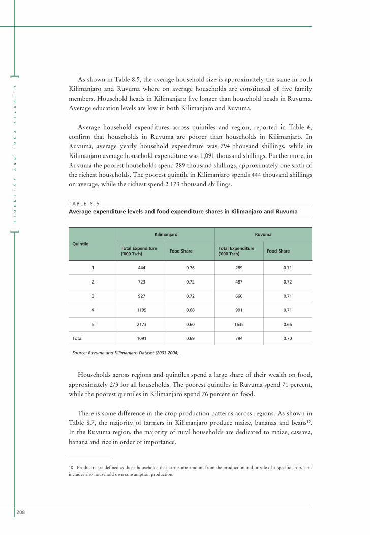
As shown in Table 8.5, the average household size is approximately the same in both Kilimanjaro and Ruvuma where on average households are constituted of five family members. Household heads in Kilimanjaro live longer than household heads in Ruvuma. Average education levels are low in both Kilimanjaro and Ruvuma.

Average household expenditures across quintiles and region, reported in Table 6, confirm that households in Ruvuma are poorer than households in Kilimanjaro. In Ruvuma, average yearly household expenditure was 794 thousand shillings, while in Kilimanjaro average household expenditure was 1,091 thousand shillings. Furthermore, in Ruvuma the poorest households spend 289 thousand shillings, approximately one sixth of the richest households. The poorest quintile in Kilimanjaro spends 444 thousand shillings on average, while the richest spend 2 173 thousand shillings.

T A B L E 8 . 6

Average expenditure levels and food expenditure shares in Kilimanjaro and Ruvuma

Quintile

Kilimanjaro Ruvuma

Total Expenditure (‘000 Tsch) Food Share Total Expenditure

(‘000 Tsch) Food Share

1 444 0.76 289 0.71

2 723 0.72 487 0.72

3 927 0.72 660 0.71

4 1195 0.68 901 0.71

5 2173 0.60 1635 0.66

Total 1091 0.69 794 0.70

Source: Ruvuma and Kilimanjaro Dataset (2003-2004).

Households across regions and quintiles spend a large share of their wealth on food, approximately 2/3 for all households. The poorest quintiles in Ruvuma spend 71 percent, while the poorest quintiles in Kilimanjaro spend 76 percent on food.

There is some difference in the crop production patterns across regions. As shown in Table 8.7, the majority of farmers in Kilimanjaro produce maize, bananas and beans10. In the Ruvuma region, the majority of rural households are dedicated to maize, cassava, banana and rice in order of importance.

10 Producers are defined as those households that earn some amount from the production and or sale of a specific crop. This includes also household own consumption production.

209


T A B L E 8 . 7

Producer and consumer numbers by crop in Kilimanjaro and Ruvuma

Producers by crop (Number of households)

Location Maize Cassava RiceSweet Potato

Sugar Banana Bean

Kilimanjaro 798 70 14 20 17 728 638

Ruvuma 841 539 281 54 6 319 399

Consumers by item (Number of households)

LocationMaize Flour

Maize Cob

Maize Grain

Cassava Dry or fresh

RiceSweet Potato

Sugar Banana Bean

Kilimanjaro 912 31 532 146 646 97 868 862 861

Ruvuma 631 221 65 717 252 49 464 363 618

There is also some difference in consumption11 across regions. Rural households in Kilimanjaro mostly consume maize flour, maize grain, rice, sugar, banana and beans. Comparatively, Ruvuma households consume more cassava and maize cob and less rice and sugar.

8.4.2 IMPACTS OF MAIZE PRICE INCREASE IN KILIMANJARO AND RUVUMAMost households in the Kilimanjaro region stand to lose from a 10 percent price increase in the price of maize, as shown in Figure 8.4. The poorer households, on average, lose 0.3 percent of their welfare upon this price increase. The middle quintile loses the most from the price increase, while the richer households benefit from the price increase.

F i g u r e 8 . 4

Welfare impacts in Kilimanjaro for a 10 percent increase in the price of maize

Source: Calculations by the authors.

11 Consumption includes both purchased foods and consumption of own production.

210

]B

IO

EN

ER

GY

A

ND

F

OO

D

SE

CU

RI

TY

[

However, as illustrated in Figure 8.5, the poorest households in Ruvuma benefit from a 10 percent price increase in the price of maize indicating that, on balance, poor households in this area grow more maize than they consume. Based on the dataset at hand, the 10 percent price increase would correspond to an approximate 0.4 percent income gain. The second lowest income quintile benefits from the price increase, but by less, approximately 0.1 percent welfare increase. The other quintiles lose from the price increase

F i g u r e 8 . 5 :

Welfare impacts in Ruvuma for a 10 percent increase in the price of maize


8.4.3 IMPACTS OF CASSAVA PRICE INCREASE IN KILIMANJARO AND RUVUMAThere is little impact from price increases in the case of Cassava in Kilimanjaro, as shown in Figure 8.6. The 10 percent price increases has a minimal positive impact on all quintiles with the exception of the wealthiest quintile. The quintile that stands to gain the most, even if minimally, is the poorest.

211


F i g u r e 8 . 6

Welfare impacts in Kilimanjaro for a 10 percent increase in the price of cassava


F i g u r e 8 . 7 :

Welfare impacts in Ruvuma for a 10 percent increase in the price of cassava


However, as illustrated in Figure 8.7, the poorer households in the Ruvuma region are negatively hit by a 10 percent increase in the price of cassava indicating that poorer households consume more cassava than they produce. The poorest quintile loses 0.2 percent of its welfare based on this price increase. The wealthier quintiles in the region benefit from the price increase. The poorer households in Ruvuma are marginally affected by price changes of sugar, banana and sweet potato.

212

]B

IO

EN

ER

GY

A

ND

F

OO

D

SE

CU

RI

TY

[

8.4.4 IMPACTS OF RICE PRICE INCREASE IN KILIMANJARO AND RUVUMA

For the sake of illustration another food staple is included in order to show how the analysis can be extended across the board to all crops. In the case of rice, all households in the Kilimanjaro region are negatively hit by a 10 percent price increase as shown in Figure 8.8.

F i g u r e 8 . 8

Welfare impacts in Kilimanjaro for a 10 percent price increase in the price of rice


As illustrated in Figure 8.8, poorer households lose on average a little more than 10 percent of their welfare. Households in the second and third quintile lose approximately 0.2 percent of their welfare. Households in the top quintile are less affected (in percentage terms).

In the case of Ruvuma as reported in Figure 8.9, increases in the price of rice are beneficial to all quintiles in the Ruvuma region. A 10 percent increase in the price of rice, increases the poorest households’ welfare by 0.3 percent. The second and third quintiles benefit significantly from the price increase too.

213


F i g u r e 8 . 9

Welfare impacts in Ruvuma for a 10 percent increase in the price of rice


How severe are the welfare impacts?As discussed in the price sections, the real percentage price changes over the last

five years were in the order of fifty percent for both maize and cassava. Consequently households over the longer period have been subject to higher percentage changes compared to the starting discussion of a 10 percent price change. Producer prices could be set to vary at 10%, 20% and then 50%. The resulting impacts would be respectively twice as high for the 20 percent change and five times as high for the 50 percent change. These percentage changes would result in significant impacts on households’ welfare.

The shortcoming of the datasetThe results presented here are only for two regions in the country and solely for

rural households. Further, taking the example of maize, we find that increases in the price of maize are positive for the Ruvuma poor but negative for poor households in the Kilimanjaro regions. This shows two shortcomings of this partial dataset. On the one hand we are unable to draw conclusions on how prices impact urban households, generally net consumers of food crops. Secondly, since we are unable to run a country level assessment, overall we do not know if an increase in the price of maize could be beneficial for households in Tanzania. For sake of illustration for example, if a country level analysis had been possible and had showed that the maize price increase were positive for the country’s welfare, the policymaker would not be concerned with the overall price increase but only with safeguarding livelihoods of particular segments of the population. In the case analyzed here, the vulnerable segment of the population would be the rural poor located in the Kilimanjaro region.

214

]B

IO

EN

ER

GY

A

ND

F

OO

D

SE

CU

RI

TY

[

8.5 CONCLUSIONSDeveloping a domestic biofuel sector takes time, in fact the establishment of a new industry typically requires a medium- to long-term perspective, but food prices in Tanzania have been changing. Changes in food prices can have a significant impact on households’ food security, especially for the most vulnerable segments of the population. In this context, it is important to realize that, while there may have been no significant bioenergy developments within the country to date, international biofuel mandates have been gaining steam. Changes in food prices are a result of international and domestic supply and demand shocks, which include additional biofuel demand. Thus, households, in the short term, can still suffer food security impacts due to domestic price movements caused by biofuel policies being implemented elsewhere. Furthermore, as argued in the chapter, medium-term and long-term food prices may rise also due to domestic biofuel policy decisions unless adequate supply response is stimulated through agriculture investment and research and development.

Consequently, from a policy perspective, it is necessary to understand how the price changes can impact the country as a whole and which price changes could affect the poor segments of the population. If the government decides to pursue the development of the bioenergy sector, there might be some short-term to medium-term trade-offs for some vulnerable segments of the population. In such a case the government might want to implement targeted safety nets for the vulnerable groups.

Although initially a wider range of crops are investigated, the analysis presented focused mainly on maize and cassava, the primary food crops in Tanzania. Price changes that could affect the country were assessed first. Secondly, actual price movements in key food crops over the medium and short term were considered and thirdly the household level welfare impacts, targeting the most vulnerable segments of the population were assessed.

Over recent years, Tanzania has fluctuated from being a slight net importer to net exporter of maize, while cassava is not a traded commodity. Maize and cassava prices have been steadily increasing in the country since 2000. Investigation of the maize and cassava price trends suggest that the maize and cassava markets are interconnected in the medium term, although less so in the short term. Between 2003 and 2008, maize and cassava prices increased approximately by 50 percent in real terms.

In the case of Tanzania, it was not possible to carry out a country representative household level analysis as the Tanzanian household budget survey does not contain detailed agriculture income by crop. Nevertheless, in order to illustrate the steps of the analysis within Module 5 and the type of questions this part of the analysis can answer, a partial dataset was used which was collected from the rural areas of the Ruvuma and Kilimanjaro regions. While this does not permit to draw conclusions at the country

215


level as it is not a country representative dataset of Tanzanian households, it allows the analysis to show which conclusions could potentially be drawn from the household level analysis.

The poorest households in Ruvuma were found to benefit from price increases in maize and rice but are negatively hit by price increases in cassava. The poorer households in Kilimanjaro are indifferent to price changes in cassava but stand to lose from price increases in maize and rice.

Although this dataset offers an example of what the analysis can accomplish it is not possible to draw country level conclusions. For example, it was not possible to assess whether price increases in maize and cassava would benefit the poor in Tanzania overall. A country level dataset would allow the analysis to determine this. There might still be some segments that lose and would potentially need to be assisted, but in view of an overall country level welfare gain.

The underlying problems remain the need to increase food production, address infrastructure needs, and invest in agriculture R&D including human capital development. A key policy recommendation therefore will be to ensure that adequate investments and/or policies are put in place to foster an environment that will allow an outward shift of the cassava supply curve that will ultimately bring the cassava price back to its original level, or even lower. If this outcome can be achieved due to sufficiently large investments in public goods, then maize imports will not increase, and might even be reduced, even though cassava is being diverted to biofuel production. However, simply using cassava to produce ethanol without simultaneously investing more in public goods will lead to higher prices and increased maize imports.

Finally, in order to ensure appropriate monitoring of the poorer and most vulnerable segments of the population, it will be essential to run the analysis presented on a country representative dataset. Furthermore, accurate cassava price data was problematical to obtain, especially for the years between 2004 and 2006. If Tanzania decides to invest in cassava for ethanol production, it will be key to monitor cassava prices closely.

216

]B

IO

EN

ER

GY

A

ND

F

OO

D

SE

CU

RI

TY

[

REFERENCESBarrett, C.B. & Dorosh, P.A., 1996, Farmer’s welfare and changing food prices: nonparametric evidence from Madagascar. American Journal of Agricultural Economics, 78 (August): 656 69.

Budd, J.W., 1993, Changing food prices and rural welfare: A nonparametric examination of the Cote d’Ivoire. Economic Development and Cultural Change, 41 (April): 587-603.

Dawe, D. C., Maltsoglou, I., 2009, Analyzing the impact of food price increases: assumptions about marketing margins can be crucial, ESA Working Paper No. 09-02, FAO

Deaton, A. 1989. Rice prices and income distribution in Thailand: A non-parametric analysis. Economic Journal, 99 (Supplement): 1-37.

Ivanic M, Martin W. 2006. Potential implications of agricultural special products for poverty in low-income countries.

Minot, N. & Goletti, F. 1998. Export liberalization and household welfare: The case of rice in Viet Nam. American Journal of Agricultural Economics, 80 (November): 738-749.

Minot, N. & Goletti, F. 2000. Rice market liberalization and poverty in Viet Nam. International Food Policy Research Institute Research Report 114. IFPRI, Washington DC.

WHAT IF THE GOVERNMENT OF TANZANIA WERE TO USE CASSAVA FOR ETHANOL PRODUCTION?In the case of the market of maize and the market of cassava, maize is a tradable1 good for which a world price exists and an open economy set-up is considered. Cassava is not a tradable commodity so the market behaves as a closed economy in this case.

First, the cassava market: current supply and demand are in equilibrium at E. If Tanzania decided to use cassava for ethanol production this would add demand and would shift the demand curve from D to D’ as shown in Figure 1b, raising the price of cassava from pc to pc’. Consequently, farmers respond to the price signal and increase production, reaching a new equilibrium in E’ (arrow 1 in Figure A.2).

1 An internationally tradable good is a good which can be traded across countries.

217

A P P E N D I X 8 A MAIZE AND CASSAVA MARKET INTERLINKAGES

218

]B

IO

EN

ER

GY

A

ND

F

OO

D

SE

CU

RI

TY

[

In the case of the maize market, domestic suppliers and consumers face the world price of maize, Pw. Domestic demand and supply are described by D and S. In the initial equilibrium, domestic supply will be equivalent to Qd+M, where Qd is the amount of production supplied by domestic producers and M is the amount imported to meet domestic demand.

Due to the biofuels induced shift in cassava demand and the consequent price increase, maize production and consumption will also respond (Figure 1a). Some farmers (but not all) will shift towards the production of cassava and out of the production of maize, while some consumers (but not all) will reduce cassava consumption and increase maize consumption. Due to this, the maize supply curve will shift inwards from S to S’, and the maize demand curve outwards, from D to D’2. The inward shift in the maize supply curve will reduce the domestic production of maize to Qd’ and increase the amount of imports to M’. Therefore, overall, the decision to use cassava for ethanol production will result in an increase in the relative price of cassava to maize, (pc/pm), and, more importantly, an increase in imports of maize.

In order to avoid an increase in maize imports, it will be crucial to ensure that the supply curve of cassava shifts out from S to S’, as shown in Figure 1a, arrow 2. This will only be possible if adequate investments in agriculture R&D, infrastructure, land expansion (or changes in policies) are implemented so that farmers can significantly increase production. Shifting the cassava supply curve out will result in a new equilibrium in the cassava market at E’’. Based on the magnitude of the shift, the new price at E’’ could be lower or higher than the original level of pc.

A key policy recommendation therefore will be to ensure that adequate investments and or policies are put in place to foster an environment that will allow the outward shift of the cassava supply curve that will ultimately bring the cassava price level back to its original level, or even lower.

If this outcome can be achieved due to sufficiently large investments in public goods, then maize imports will not increase, and might even be reduced, even though cassava is being diverted to biofuel production. However, simply using cassava to produce ethanol without simultaneously investing more in public goods will lead to more maize imports.

2 The magnitude of the maize price change will be determined by the magnitude of the price change for cassava (which will depend on the size of the target for biofuel production) and by the cross-price elasticities of demand and supply between maize and cassava (which measure how consumers and farmers can shift between the two crops).

219

APPENDIX 8A: MAIZE AND CASSAVA MARKET INTERLINKAGES

WHAT IF “NEW LAND” WERE TO BECOME AVAILABLE?

In the case that new land is available for all of the cassava devoted to biofuel production, the shift in demand would be accompanied by an equivalent shift in supply and there would be no change in the price of cassava (Figure 1c and 1d). In this case, the maize market would not be affected, and there would be no increase in maize imports. The availability of new land, however, would obviously rely on suitable investment to make the new land exploitable. Thus, the importance of investment is again clear. Attention should also be given to any environmental effects of exploiting new land, as well as effects on the land rights of the poor.

220

A P P E N D I X 8

METHODOLOGICAL BACKGROUND FOR THE ASSESSMENT OF NET HOUSEHOLD WELFARE IMPACTS.

B

An outline of the procedure used to calculate the net welfare impacts of price changes at the household level is given here. For the full technical details the reader is referred to the complete BEFS Analytical Framework (forthcoming) and Dawe and Maltsoglou (2009).1

The methodology was initially set up by Deaton (1989), then followed by a number of empirical applications by other authors including Budd (1993), Barrett and Dorosh (1996), Minot and Goletti (1998, 2000) and, recently, Ivanic and Martin (2008). Here the methodology has been applied as described in Minot and Goletti (2000).

The impact of a price change on household welfare can be decomposed into the impact on the household as a consumer of the goods and the impact on the household as a producer of the goods. The net welfare impact will be the difference between the two. Therefore if the demand and supply side elasticities are set to equal zero, thus ignoring consumer and producer side response to price changes, the short run welfare impact on households is calculated as

=%PP . PR - %PC

. CRi (1)�w1

i

x0i

where �w1

i

x0i is the first order approximation of the net welfare impact on producer and

consumer households deriving from a price change in commodity i, relative to intial total income x0i (in the analysis income is proxied by expenditure)

%PP is the change in producer price for commodity i

PRi is the producer ratio for commodity i and is defined as the ratio between the value of production of i to total income (or total expenditure)

%PC is the change in consumer price for commodity i.

CRi , is the consumer ratio for commodity i and is defined as the ratio between total expenditure on commodity i and total income (or total expenditure)

1 For a detailed discussion on this summary appendix the reader is referred to Dawe and Maltsoglou (2009).

221

APPENDIX 8B: METHODOLOGICAL BACKGROUND FOR THE ASSESSMENT OF NET HOUSEHOLD WELFARE IMPACTS

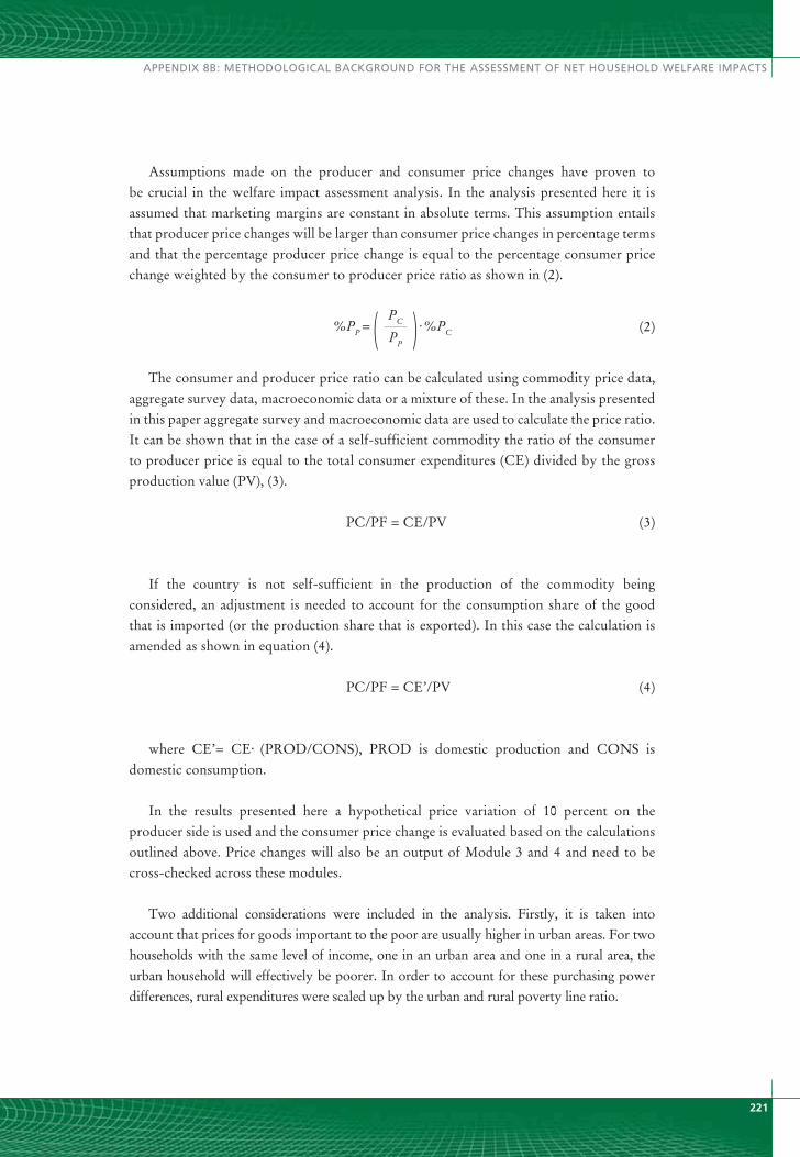
Assumptions made on the producer and consumer price changes have proven to be crucial in the welfare impact assessment analysis. In the analysis presented here it is assumed that marketing margins are constant in absolute terms. This assumption entails that producer price changes will be larger than consumer price changes in percentage terms and that the percentage producer price change is equal to the percentage consumer price change weighted by the consumer to producer price ratio as shown in (2).

.%PC%PP =

PC

PP ( ) (2)

The consumer and producer price ratio can be calculated using commodity price data, aggregate survey data, macroeconomic data or a mixture of these. In the analysis presented in this paper aggregate survey and macroeconomic data are used to calculate the price ratio. It can be shown that in the case of a self-sufficient commodity the ratio of the consumer to producer price is equal to the total consumer expenditures (CE) divided by the gross production value (PV), (3).

PC/PF = CE/PV

(3)

If the country is not self-sufficient in the production of the commodity being considered, an adjustment is needed to account for the consumption share of the good that is imported (or the production share that is exported). In this case the calculation is amended as shown in equation (4).

PC/PF = CE’/PV (4)

where CE’= CE. (PROD/CONS), PROD is domestic production and CONS is domestic consumption.

In the results presented here a hypothetical price variation of 10 percent on the producer side is used and the consumer price change is evaluated based on the calculations outlined above. Price changes will also be an output of Module 3 and 4 and need to be cross-checked across these modules.

Two additional considerations were included in the analysis. Firstly, it is taken into account that prices for goods important to the poor are usually higher in urban areas. For two households with the same level of income, one in an urban area and one in a rural area, the urban household will effectively be poorer. In order to account for these purchasing power differences, rural expenditures were scaled up by the urban and rural poverty line ratio.

222

]B

IO

EN

ER

GY

A

ND

F

OO

D

SE

CU

RI

TY

[

Secondly, based on the selected commodity list, crops produced at the farm level might be very different compared to the commodity actually consumed by the households. Clear examples of this are wheat and maize. Wheat is produced at the farm level, but consumers eat bread, biscuits or purchase wheat flour. Maize is slightly more complex since maize produced on the farm can either be used for human consumption (white maize) or used for feed (yellow maize). All commodities generally have some degree of processing embedded in them which varies according to which commodity is under scrutiny. Based on discussions with experts in FAO, some rules of thumb have been set up for what the processing factors may be and these have been used in this paper (Table B.1). Again, a more detailed discussion on processing is presented in Dawe and Maltsoglou (2009).

T A B L E B . 1

Subproduct factors used to calculate the net welfare impacts at household level.

Commodities Subproduct or Description Share in Value Ratio *

Maize Chicken 20

Eggs 20

Pigs 10

Flour 60

Cobb 75

Grain 75

Cassava Fresh 50

Dry 50

Rice 65

Sweet potato 50

Sugar 20

Plantains 50

Beans 65

Source: FAO, 2009* This is the ratio of the final product to the farm gate product.

8 HOUSEHOLD LEVEL FOOD SECURITY AND VULNERABILITY

Documents

Transcript of 8 HOUSEHOLD LEVEL FOOD SECURITY AND VULNERABILITY