
8 Channels

8.1 INTRODUCTION

Open channels are natural or human-made conveyance systems for water, stormwater, and flood

water in which the water is exposed to the atmosphere, and the driving force is the force of gravity

in the direction of motion. The design of transportation facilities and appurtenances for open-

channel-flow conveyance encounters various types of channels including streams, creeks, rivers,

roadside ditches or swales, irrigation facilities, drainage sloughs, and other waterways that are

natural or human-made, or a combination of both. Some of these are illustrated in Photos 8.1

through 8.4 below.

Photo 8.1 (upper left) Spring Creek at US 287 in Fort Collins, showcasing an urban waterway

entering CDOT right-of-way.

Photo 8.2 (upper right) Roadside swale on northbound SH 93 in Boulder County being inspected

for erosion damage and water-quality maintenance.

Photo 8.3 (lower left) Riprap installation on the banks of the Little Thompson River at SH 60 in

Milliken during a bridge-replacement project and permanent repair work following the 2013 flood

disaster.

Photo 8.4 (lower right) A grassy swale maintained along the northbound lane of SH 113 near Peetz,

showing the benefits of erosion protection from well-established and maintained natural vegetation.


Channel analysis is important for the design of effective roadside-drainage systems and structural

crossings of creeks, streams and rivers. In the process of hydraulic design associated with natural

channels and roadway ditches, the engineer selects and evaluates alternatives according to

established criteria. These criteria are standards established by CDOT to ensure that a highway

facility meets its intended purpose without endangering the structural integrity of the facility itself,

and with minimal adverse effects on the environment or public welfare.

It is the purpose of this chapter to identify open-channel-flow behaviors and relationships, establish

CDOT design criteria, outline procedures for efficient channel design, and provide cross-referenced

guidance to other chapters in this manual for the safe and efficient management of stormwater and

flood waters in and near Colorado transportation corridors.

8.2 OPEN-CHANNEL FLOW DEFINITIONS

This section provides a summary of hydraulic terms and concepts integral to understanding open-

channel flow. For further discussion, consult Chow’s Open Channel Hydraulics (1959), the

Hydraulic Engineering Center’s River Analysis System Hydraulics Reference Manual (2016), and

FHWA Hydraulic Design Series No. 4 (HDS-4), Introduction to Highway Hydraulics (2008).

Conveyance: the quantifiable capacity of a channel to move flow from one location to another

under the force of gravity.

Froude Number, Fr: represents the ratio of inertial forces to gravitational forces, or cross section

average-flow velocity to the celerity of flow in an open channel.

Critical Flow: a specific flow behavior that occurs when the specific energy is the minimum for

a given discharge in regular channel cross sections. The depth at which the specific energy is

minimum is called the critical depth. At the critical depth, the Froude number has a value of 1.0 at

that specific location within a reach. The critical depth is also the depth of maximum discharge

when the specific energy is held constant.

Hydraulic Jump: a hydraulic jump occurs as an abrupt transition from supercritical to subcritical

flow in the direction of the flow. There are significant changes in depth and velocity in the jump,

and energy is dissipated over the effective length of the jump. These features are highly erosive,

but quite effective at dissipating energy and transitioning flows to a more stable subcritical regime

at highway drainage structures. When a hydraulic jump is used as an energy dissipator, controls to

create sufficient tailwater depth are often necessary to confine the location of the jump over a range

of discharges. More information for hydraulic jump design is available in Chapter 11– Energy

Dissipators.

Normal Depth: the occurrence of normal depth is unique for a given channel geometry, slope,

roughness, and discharge during steady, uniform flow. Normal depth assumes a channel is

prismatic along a long reach, there are no discernable changes in land use or materials, boundaries

are rigid, radii of curvature are negligible, and no hydraulic structures exist within the reach. If the

normal depth is greater than critical depth, the slope is classified as a mild slope. If the normal

depth is less than critical depth, the slope is classified as a steep slope. Natural channels vary in

topography, roughness, shape and slope over short distances and rarely exhibit long reaches of

normal depth in Colorado. But, during the design of human-made channels, a normal depth

condition is frequently assumed for calculations. This must be confirmed in practice and verified

in review.

Specific Energy, E: defined as the energy head relative to the channel bottom. In mildly-sloped

channels where the longitudinal slope is generally less than one percent (1%), and the streamlines


are nearly straight and parallel (so that the hydrostatic assumption holds), the specific energy is the

sum of the depth and velocity head.

Stage: measured water-surface elevation at a given location with a known or otherwise calculated

bed elevation, often (though incorrectly) expressed as a substitute for depth.

Steady Flow: discharge passing a given cross section is constant with respect to time.

Subcritical Flow: gradually varied flow behavior where flow is generally categorized as slow and

deep. In a subcritical flow reach, the Froude Number is less than 1.0 and the depth of flow at a

given location is greater than critical depth. In this state of flow, small water-surface disturbances

can travel both upstream and downstream, and the control is always located downstream.

Supercritical Flow: a gradually varied flow behavior where flow is generally categorized as fast

and shallow. Subcritical flow exhibits Froude Numbers greater than 1.0 and depths are more

shallow than critical depth. Small water-surface disturbances are always swept downstream in

supercritical flow, and the location of the flow control is always located upstream. Supercritical

flow is highly erosive and unstable in natural channels, roadside swales, and other human-made

open channels, and should be avoided for design purposes unless the energy of the flow can be

safely and adequately dissipated (see Chapter 11 – Energy Dissipators).

Unsteady Flow: the discharge passing a given cross section varies with respect to time.

8.3 OPEN-CHANNEL FLOW EQUATIONS

The design and analysis of both natural and constructed channels proceed according to the basic

principles of open-channel flow (see Chow’s Open Channel Hydraulics, and Henderson’s Open

Channel Flow). The basic principles of fluid mechanics (e.g., continuity, momentum, energy) can

be applied to open-channel flow with the additional complication that the position of the free

surface is usually one of the unknown variables. The determination of this unknown is one of the

primary objectives of open-channel flow analysis.

Specific Energy, E: the specific energy of open channel flow. It is the sum of the depth and

velocity head, expressed in Equation 8.1 as follows:

𝐸 = 𝑦 + 𝛼𝑉2

2𝑔 (8.1)

where: E = Specific Energy (ft)

y = depth (ft)

α = velocity distribution coefficient (1.13 to 1.40 for prismatic channels)

V = cross section average-flow velocity (ft/s or fps)

g = acceleration due to gravity (32.2 ft/s2)

Froude Number: the Froude number is generally expressed as the ratio expressed in Equation

8.2:

𝐹𝑟 =𝑉

√𝑔𝐷 (8.2)


where: V = Q/A, = cross section average flow velocity (ft/s or fps)

Q = total discharge (ft3/s or cfs)

A = cross section average-flow area (ft2)

G = acceleration due to gravity (32.2 ft/s2)

D = A/T = hydraulic depth (ft)

T = channel top width at water surface (ft)

Critical Flow: the general cross sectional relationship for a one-dimensional, prismatic channel,

critical depth is expressed in Equation 8.3:

𝑄2

𝑔=

𝐴3

𝑇 (8.3)

where: Q = total discharge (ft3/s or cfs)

g = acceleration due to gravity (32.2 ft/s2)


T = channel top width at water surface (ft)

Continuity Equation: the Continuity Equation is the statement of conservation of mass in fluid

mechanics. For the special case of one-dimensional steady flow of an incompressible fluid it

assumes the simple form of Equation 8.4:

Q = AV (8.4)



V = cross section average-flow velocity (ft/s or fps)

Manning’s Equation: for a given depth of flow in an open channel with steady, uniform flow,

the cross section average-flow velocity in the principle flow direction can be computed with

Manning’s Equation expressed in Equation 8.5:

𝑉 =1.486

𝑛𝑅2∕3𝑠𝑓

1∕2 (8.5)

where: V = cross section average flow velocity (ft/s or fps)

R = A/P = hydraulic radius (ft)


P = wetted perimeter (ft)

Sf = friction slope, assumed to be the same as bed slope (ft/ft)

The continuity equation can be combined with Manning’s equation to express the steady, uniform-

flow discharge more commonly used for design in the form of Equation 8.6:

𝑄 =1.486

𝑛𝐴𝑅2∕3𝑠𝑓

1∕2 (8.6)


n = Manning’s roughness coefficient (L1/6, or essentially unitless)


R = hydraulic radius (ft)


For a given channel geometry, slope, roughness, and discharge, a unique value of depth occurs in

steady, uniform flow. This unique depth is referred to as normal depth and is computed from

Equation 8.6 after the area and hydraulic radius are expressed in terms of depth.


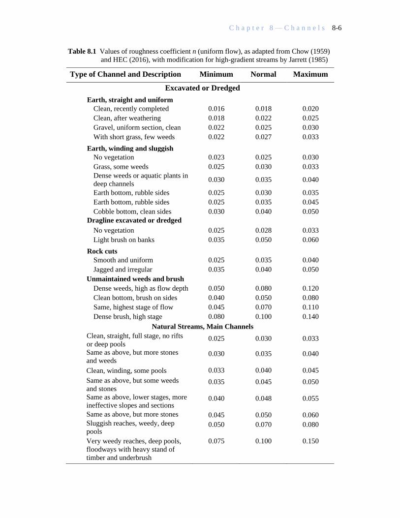
Table 8.1 Values of roughness coefficient n (uniform flow), as adapted from Chow (1959)

and HEC (2016), with modification for high-gradient streams by Jarrett (1985)

Type of Channel and Description Minimum Normal Maximum

Excavated or Dredged

Earth, straight and uniform

Clean, recently completed 0.016 0.018 0.020

Clean, after weathering 0.018 0.022 0.025

Gravel, uniform section, clean 0.022 0.025 0.030

With short grass, few weeds 0.022 0.027 0.033

Earth, winding and sluggish

No vegetation 0.023 0.025 0.030

Grass, some weeds 0.025 0.030 0.033

Dense weeds or aquatic plants in

deep channels 0.030 0.035 0.040

Earth bottom, rubble sides 0.025 0.030 0.035

Earth bottom, rubble sides 0.025 0.035 0.045

Cobble bottom, clean sides 0.030 0.040 0.050

Dragline excavated or dredged

No vegetation 0.025 0.028 0.033

Light brush on banks 0.035 0.050 0.060

Rock cuts

Smooth and uniform 0.025 0.035 0.040

Jagged and irregular 0.035 0.040 0.050

Unmaintained weeds and brush

Dense weeds, high as flow depth 0.050 0.080 0.120

Clean bottom, brush on sides 0.040 0.050 0.080

Same, highest stage of flow 0.045 0.070 0.110

Dense brush, high stage 0.080 0.100 0.140

Natural Streams, Main Channels

Clean, straight, full stage, no rifts

or deep pools 0.025 0.030 0.033

Same as above, but more stones

and weeds 0.030 0.035 0.040

Clean, winding, some pools 0.033 0.040 0.045

Same as above, but some weeds

and stones 0.035 0.045 0.050

Same as above, lower stages, more

ineffective slopes and sections 0.040 0.048 0.055

Same as above, but more stones 0.045 0.050 0.060

Sluggish reaches, weedy, deep

pools 0.050 0.070 0.080

Very weedy reaches, deep pools,

floodways with heavy stand of

timber and underbrush

0.075 0.100 0.150


Table 8.1 Continued

Type of Channel and Description Minimum Normal Maximum

Natural Streams, Flooded Overbanks

Pasture, no brush

Short grass 0.025 0.030 0.035

High grass 0.030 0.035 0.050

Cultivated area

No crops 0.020 0.030 0.040

Mature crops 0.025 0.035 0.050

Brush

Scattered brush, heavy weeds 0.035 0.050 0.070

Light brush and trees in winter 0.035 0.050 0.080

Light brush and trees in summer 0.040 0.060 0.080

Medium to dense brush in winter 0.045 0.070 0.110

Medium to dense brush in

summer 0.070 0.100 0.160

Trees

Cleared land with tree stumps,

no sprouts

0.030 0.040 0.050

Same as above, but heavy

sprouts

0.050 0.060 0.080

Heavy stand of timber, a few

downed trees, little undergrowth,

flow below branches

0.080 0.100 0.120

Same as above, but with flow

into branches

0.100 0.120 0.160

Dense willows in summer,

straight

0.110 0.150 0.200

Mountain Streams, Steep Longitudinal Slopes, No Vegetation in

Channel, Steep Banks, with Submerged Trees and Brush on Banks

Bottom; gravels, cobbles, and a few boulders Use Jarrett’s Equation

Bottom; cobbles with large boulders Use Jarrett’s Equation

Note the adaptation of Jarrett’s Equation for natural mountain streams with steep gradients and

large substrates. The methodology for steep-gradient systems differs from lower-gradient streams

due in large part to turbulence (vertical and horizontal), rapidly-varied flow, and air entrainment.

Equation 1 from Jarrett tends to produce roughness coefficients in reaches of turbulent exchange

that more closely match observed hydraulic behaviors. Jarrett’s Equation 1 is included in Volume

1, Chapter 8 of the Urban Drainage and Flood Control District’s (UDFCD) Urban Storm Drainage

Criteria Manual (Wright Water Engineers, 2016), and is reproduced here as Equation 8.7 for

determining roughness coefficients for cobble- and riprap-lined streams in Colorado:


𝑛 = 0.39 𝑆𝑓0.38 𝑅−1∕6 (8.7)

where: n = Manning roughness coefficient (L1/6, or essentially unitless)

R = A/P = hydraulic radius (ft)


Manning’s n is affected by many factors. Pictures of channels and floodplains for which the

discharge has been measured and Manning’s n has been calculated are useful. For situations outside

the engineer’s experience, a more-formal approach is presented in USGS Water-Supply Paper

2339, “Guide for Selecting Manning’s Roughness Coefficients for Natural Channels and Flood

Plains.” Photographic information is also provided in USGS Water-Supply Paper 2849,

“Roughness Characteristics of Natural Channels” (Barnes, 1967). Once Manning’s n values have

been selected, it is recommended that they be verified with historical high-water marks and/or

gaged-streamflow data. Recommended n values are provided by default in FHWA’s Hydraulic

Toolbox (see Section 8.6 - Software for Modeling Channels and Floodplains).

Conveyance: one of the most important variables for design of open channels is conveyance. In

channel analysis, it is often convenient to group the channel cross-section properties of Equation

8.6 in a single term called the channel conveyance expressed as Equation 8.8:

𝐾 =1.486

𝑛𝐴𝑅2∕3 (8.8)

When combined with Equations 8.4 and 8.5, conveyance clearly becomes a contributing factor to

the calculation of discharge in channel design succinctly represented by Equation 8.9:

Q = K S1/2 (8.9)

Energy Equation: the conservation of energy in open-channel flow is expressed as energy per

unit weight of fluid, which has dimensions of length, and is therefore called energy head. The

energy head is composed of potential energy head (or elevation), pressure head (or stage), and

kinetic energy head (or velocity head). These energy heads are scalar quantities that give the total

energy head at any cross section using the Energy Equation. Written between an upstream open-

channel cross section designated 1 and a downstream open-channel cross section designated 2 (see

Figure 8.1), the Energy Equation takes the form of Equation 8.10:

𝑦1 + 𝑧1 + 𝛼𝑉1

2

2𝑔= 𝑦2 + 𝑧2 + 𝛼

𝑉22

2𝑔+ ℎ𝐿 (8.10)

where: y1, y2 = upstream and downstream maximum flow depths, respectively (ft)

V1, V2 = upstream and downstream average flow velocities, respectively (ft/s or fps)

Α = velocity distribution coefficient (1.13 to 1.40 for prismatic channels)

g = acceleration due to gravity (32.2 ft/s2).

hL = head loss (ft, typically friction, contraction and expansion losses)


Figure 8.1. Terms in the energy equation (source: HDS-4, 2008)

The Energy Equation illustrates that the total energy head at an upstream cross section is equal to

the energy head at a downstream section plus the head losses between these two sections. The

equation can only be applied between two cross sections at which the streamlines are nearly straight

and parallel so that vertical accelerations and lateral exchanges can be neglected.

8.4 DESIGN CRITERIA AND GUIDELINES

Standard open channel design criteria are identified in Table 8.2 for roadside drainage swales and

natural channels, but are not to be used to design energy dissipators (see Chapter 11), culverts (see

Chapter 9), storm sewers or rundowns (see USDCM, 2016).

Table 8.2 Standard open channel design criteria on CDOT projects (not an exhaustive list)

Standard Design

Parameter

Grass-Lined

Swales

Riprap

Swales

Natural

Channels

Alternative

References

Longitudinal slope (max.) 0.6% 1.0% 0.5% HEC-15 and

USDCM

Longitudinal slope (min.) 0.2% 0.2% Match

Adjacent

HEC-15 and

USDCM

Depth (max.) 5.0 ft 5.0 ft Variable HEC-23 and

USDCM

Sideslope (H:V, max.) 3.0:1 2.5:1 2.5:1 HEC-15, HEC-23

and USDCM

Froude Number (max.) 0.60 0.80 0.60 HEC-15 and

USDCM

Freeboard (min.) 1.0 ft 1.0 ft See Chapter 10 Chapter 10 and

USDCM


Further guidance in association with Table 8.2 standard design criteria:

• Embankment encroachment in any stream channel or floodplain should be avoided,

especially in regulatory floodplains and floodways (see Chapter 2).

• If encroachment into a regulatory floodplain cannot be avoided, the hydraulic effects of the

encroachment on any major highway facility must be evaluated over a full range of

frequency-based peak discharges, including: the 2-, 5-, 10-, 25-, 50-, 100- and 500-yr

recurrence intervals; any project-specific design flood; the regulatory base flood (typically

the same as the 100-yr recurrence interval); the incipient overtopping flood condition; and,

any other recurrence interval required by federal, state, regional, tribal or local standards

for master planning and floodplain-development permitting.

• Bends should have radii of curvature comparable to those encountered in the natural bends

in the channel vicinity. The minimum radius of curvature for bends designed to operate

under subcritical flow conditions should be determined using methods outlined in the

USDCM (2016).

• Flexible linings for small roadside channels should be designed according to the method

of allowable tractive force, and conform with criteria found in FHWA Hydraulic

Engineering Circular No. 15 (HEC-15, 2005), “Design of Roadside Channels with Flexible

Linings.” Refer to Chapter 17 - Bank Protection and HEC-23 for revetment design methods

for larger man-made channels and natural streams.

• Roadside channel linings must be designed for interim conditions during and immediately

after construction, and for a long-term condition with full vegetation density (typically

75%). All roadside channel linings must conform with CDOT M&S Standards, and with

product specifications provided by manufacturers to ensure proper installation,

maintenance, layering, and long-term viability of selected products. In many cases,

temporary linings, mulch, or other treatments may be required to provide stability until

required final post-construction vegetation density is established over a period of months

or years.

• The design discharge for permanent roadside-ditch linings and revetments should match

the design frequencies identified in Table 7.2 (see Chapter 7).

• Energy dissipators should be designed using Hydraulic Engineering Circular No. 14 (HEC-

14), “Hydraulic Design of Energy Dissipators for Culverts and Channels” (2006, see

Chapter 11).

• Environmental considerations of working in natural streams are presented in Chapter 15.

Hydraulic conditions in a drainage channel can present risks to the safety of the traveling public

and CDOT infrastructure assets even on mildly-sloped waterways. As a result, most open channels

require some level of stabilization against erosion, headcutting, lateral migration, aggradation,

degradation and scour. The following series of FHWA resources (not an exhaustive list) provide

design procedures and guidance for the analysis, design, and construction of features that protect

highway user safety and DOT assets from detrimental impacts of water in the natural and built

environment. They also provide strategies to support infrastructure design that accommodates and

enhances ecological and fluvial geomorphologic functions of natural waterways.

• HEC-18 (2012) – “Evaluating Scour at Bridges,” scour calculation and mitigation methods;

• HEC-20 (2012) “Stream Stability at Highway Structures,” stream-stability assessments;

• HEC-23 (2009) – “Bridge Scour and stream Instability Countermeasures Experience,

Selection and Design Guidance” (volumes 1 and 2), analysis and design of larger channels

(both human-made and natural), creeks, rivers and waterways larger than roadside swales.

This resource includes design and construction standards for riprap, matrix riprap,


guidebanks and other channel protection features. It also includes design and construction

standards for scour countermeasures for bridges analyzed with HEC-18 methods.

• HDS-4 (2008) – “Introduction to Highway Hydraulics,” fundamental hydraulic analysis

and design manual for highways;

• HDS-5 (2012) – “Hydraulic Design of Highway Culverts,” culvert analysis, design and

construction manual (see Chapter 9); and

• HDS-7 (2012) – “Hydraulic Design of Safe Bridges,” a hydraulic design compendium for

bridge safety.

8.5 HYDRAULIC ANALYSIS

The hydraulic analysis of both natural and human-made channels relies on basic principles of open

channel and fluid mechanics, primarily the continuity of energy and continuity of momentum. The

hydraulic analysis of a channel determines the depth and velocity at which a given discharge will

flow in a channel of known geometry, roughness, and slope. From these variables many other

defining hydraulic properties can be quantified. Good channel design consists of the proper

selection of capacity, freeboard, alignment, erosion resistance, and aesthetics, all of which can be

checked against the standard criteria of Table 8.2.

The two methods most commonly used in hydraulic analysis of open channels are the single-section

method, and the step-backwater method. The single-section method (also known as the normal-

depth method) applies Manning’s equation to determine tailwater rating curves for culverts, or to

analyze other situations in which uniform, or nearly uniform, flow conditions exist. The step-

backwater method is used to compute the complete water-surface profile for a stream reach, or to

analyze other gradually-varied flow situations in open channels.

The single-section analysis method (also known as slope-area method or normal-depth calculation)

involves solving Manning’s equation for the normal depth of flow given discharge, geometry, slope

and roughness of cross-sections. It assumes the existence of steady, uniform flow, and is commonly

applied to the design of roadside ditches and culverts used for local drainage.

The step-backwater analysis method, or standard-step method, uses the energy equation to “step”

the stream water surface along the profile. This method is commonly referred to as a one-

dimensional analysis, and is typically more accurate than the slope-area method for calculating

water surface profiles for steady, gradually-varied flow. Both subcritical and supercritical flow

profiles can be calculated, and since calculations can be repetitive in a long study reach, it is

recommended that computer programs such as the HEC-RAS Version 5.0 (2016) or FHWA’s

Hydraulics Toolbox (2018) be utilized.

The preparation of step-backwater analyses can be time consuming, and it is always beneficial to

search for existing studies and background information before analysis. Existing studies and

boundary condition information can be obtained from CDOT hydraulic engineers and resident

engineers, or from other governmental partnering agencies, including:

• FHWA Resource Center;

• Federal Emergency Management Agency (FEMA) Region VIII;

• FEMA’s Map Service Center (MSC at msc.fema.gov);

• Colorado Water Conservation Board (CWCB);

• UDFCD and partnering local entities; and

• Local floodplain administrators (county, town or city)


Open-channel flow problems sometimes arise that require a more-detailed analysis than a single-

section analysis, or the computation of a water-surface profile using the Standard-Step Method or

Direct-Step Method. More-detailed analysis techniques include two-dimensional (2D) analysis,

water and sediment routing, and unsteady flow analysis in 1D and 2D. Resources for these analyses

can include HEC-RAS Version 5.0 or most current (2016) and Aqueveo’s Surface-water Modeling

System Version 12 or most current (SMS 13.0, 2018). Local or regional agency requirements may

revert to legacy software depending on jurisdictional requirements, and will be managed on a case-

by-case basis with regulators. Information on available hydraulic analysis software is provided in

Section 8.7, and in HDS-7, Table 4.1 (2012).

8.6 SOFTWARE FOR MODELING CHANNELS AND FLOODPLAINS

The software identified in Tables 8.3 and 8.4 were the most recent when this manual was prepared.

For current versions of software and documentation, the hydraulic engineer should consult the

software source, or confer with local agencies in project jurisdictions to ensure seamless transition

of design analyses during CDOT project-delivery activities.

Roadside channels, culvert tailwater channels, and constructed channels that have a uniform cross

section can be assessed using a single representative cross section and the channel slope. FHWA

Hydraulic Toolbox, the WMS channel calculator (Aquaveo 2018), or HEC-RAS (HEC 2016)

software are useful for calculating steady, uniform flow using Manning’s equation combined with

the continuity equation.

If the channel does not have a uniform cross section in the direction of flow, then a one-dimensional

hydraulic-analysis program can be utilized. One-dimensional hydraulic models are characterized

by a series of cross sections placed perpendicular to the predominantly-downstream flow direction

to represent topography. Boundary conditions placed at both ends of the simulation are then

analyzed using the step-backwater analysis procedure. Hydraulic properties for cross sections of

interest can be easily extracted to design bank protection or other countermeasures to protect

against bank erosion, lateral migration, channel degradation, and scour.

Natural channels or streams with complex alignments or that interact with highway conveyance

structures cannot always be adequately represented by a series of cross sections perpendicular to

the assumed direction of flow. For these complex-flow conditions, the waterway should be

analyzed with a two-dimensional hydraulic analysis that utilizes a higher-order or more-granular

solution. Two dimensional analysis can be an effective tool for quantifying complex flow behaviors

associated with design, maintenance and planning efforts.

There are two primary graphical user interfaces for computing two-dimensional hydraulic analyses,

Aquaveo’s SMS, and the U.S. Army Corps of Engineers’ HEC-RAS, both of which are summarized

in Table 8.4. The U.S. Bureau of Reclamation’s Sedimentation and River Hydraulics (SRH-2D)

program is specifically endorsed by FHWA as a two-dimensional hydraulic model specifically

oriented toward transportation hydraulic engineering, that calculates depth-averaged hydraulics,

sediment, temperature, and vegetation for natural and human-made open channels.

The results from two-dimensional models provide highly-detailed analyses for design channels,

channel revetments, scour countermeasures, bank protection, and stream rehabilitation features.

HDS-7, Table 4.1 (2012) is a useful tool for deciding which hydraulic analysis is most appropriate

for use on a CDOT project. New guidance is anticipated to be released by the FHWA Resource

Center in 2019 to provide detailed guidance in the proper selection of analytical tools for hydraulic

analysis of waterways in and near infrastructure assets.


Table 8.3 One-dimensional hydraulic modeling software

Table 8.4 Two-dimensional hydraulic modeling software

Software

Name Software Features Source

SMS The Surface Water Modeling System (SMS) is a comprehensive

environment for one- and two-dimensional hydrodynamic modeling. A

pre- and post-processor for surface-water modeling and design, SMS

includes two-dimensional finite element and finite difference analyses,

and finite volume analysis with the addition of SRH-2D.

The FHWA analysis package SRH-2D includes options for modeling

bridges, culverts and highways in three-dimensions with two-

dimensional output. This is the preferred software package for 2D

hydraulic models of bridges in and near CDOT-managed highway

systems.

Aquaveo

website

HEC-RAS HEC-RAS contains one- and two-dimensional hydrodynamic modeling

capabilities in steady and unsteady flow environments. Sediment

transport capabilities are available within the program that is expected

to evolve quickly.

HEC

website

The software shown in Tables 8.3 and 8.4 are updated periodically. The most recent versions of

these software are recommended for use. For current versions of software and documentation, the

hydraulic engineer should consult the software source.

Software

Name Software Features Source

HEC-RAS HEC-RAS contains four one-dimensional river analysis components for

steady-flow water-surface-profile computation, unsteady-flow simulation,

moveable- boundary sediment-transport computations, and water- quality

analysis. Release 5 also includes two-dimensional analysis and GIS-ready

functions with RAS-Mapper, and enhanced scour calculation functions.

HEC

website

FHWA

Hydraulic

The FHWA Hydraulic Toolbox Program is a stand-alone suite of

calculators that performs routine hydrologic and hydraulic computations.

The program allows a user to perform and save hydraulic calculations in

one project file, analyze multiple scenarios, and create plots and reports

of these analyses. The computations can be carried out in either CU or SI

units. Twelve calculators are available for a variety of calculations

provided in HDS-2, HEC-14, HEC-15, HEC-22, and HEC-23.

FHWA

website

WMS

Channel

Calculator

The Channel Calculator is a feature of the WMS, Hydrologic Modeling

Module. One clicks on Calculators on the Menu Tool Bar to display the

available calculators. The Channel Calculator determines the shear stress

for a given discharge, and uses the allowable shear stress for the lining

selected to determine the safety factor. WMS provides interfaces to the

latest versions of HY-8 and the Hydraulic Toolbox distributed by FHWA.

Aquaveo

website


REFERENCES

1. Aquaveo, Watershed Modeling System (WMS), Version 10.1, 2018.

2. Aquaveo, Surface-water Modeling System (SMS), Version 12.3, 2018.

3. Arcement, G.J. Jr., and Schneider, V.R., “Guide for Selecting Manning’s Roughness

Coefficients for Natural Channels and Flood Plains,” Water-Supply Paper 2339, U.S.

Geological Survey, U.S. Department of Transportation and Federal Highway Administration,

Denver, CO, 1989.

4. “Guide for Selecting Manning’s Roughness Coefficients for Natural Channels and Flood

Plains,” Report No. FHWA TS 84 204, Federal Highway Administration, 1989.

5. Barnes, H.H. Jr., “Roughness Characteristics of Natural Channels,” USGS Water Supply

Paper 1849, U.S. Geological Survey, Washington D.C., 1967.

6. Chow, V.T., Open Channel Hydraulics, McGraw Hill, New York, NY, 1959.

7. Federal Highway Administration, Highway Hydrology, Hydraulic Design Series No. 2 (HDS-

2), Second Edition, FHWA-NHI-02-001, National Highway Institute, Arlington, VA, 2002.

8. Federal Highway Administration, Introduction to Highway Hydraulics, Hydraulic Design

Series No. 4 (HDS-4), Third Edition, FHWA-HIF-12-026, National Highway Institute,

Washington D.C., 2008.

9. Federal Highway Administration, Hydraulic Design of Highway Culverts, Hydraulic Design

Series No. 5 (HDS-5), Fourth Edition, FHWA-NHI-08-090, National Highway Institute,

Arlington, VA, 2012.

10. Federal Highway Administration, River Engineering for Highway Encroachments -

Highways in the River Environment, Hydraulic Design Series No. 6 (HDS-6), FHWA-NHI-

01-004, Federal Highway Administration, U.S. Department of Transportation, Washington

D.C., 2001.

11. Federal Highway Administration, “Hydraulic Design of Energy Dissipators for Culverts and

Channels,” Hydraulic Engineering Circular No. 14 (HEC-14), Third Edition, FHWA-NHI-

06-086, National Highway Institute, Arlington, VA, 2006.

12. Federal Highway Administration, “Design of Roadside Channels with Flexible Lining,”

Hydraulic Engineering Circular No. 15 (HEC-15), Third Edition, FHWA-NHI-05-114,

National Highway Institute, Arlington, VA, 2005.

13. Federal Highway Administration, “Highways in the River Environment - Floodplains,

Extreme Events, Risk, and Resilience,” Hydraulic Engineering Circular No. 17 (HEC-17),

Second Edition, FHWA-HIF-16-018, Office of Bridges and Structures, Washington D.C.,

2016.

14. Federal Highway Administration, “Evaluating Scour at Bridges,” Hydraulic Engineering

Circular No. 18 (HEC-18), Fifth Edition, FHWA-HIF-12-003, National Highway Institute,


15. Federal Highway Administration, “Stream Stability at Highway Structures,” Hydraulic

Engineering Circular No. 20 (HEC-20), Fourth Edition, FHWA-HIF-12-004, National

Highway Institute, Arlington, VA, 2012.

16. Federal Highway Administration, “Urban Drainage Design Manual,” Hydraulic Engineering

Circular No. 22 (HEC-22), Third Edition, FHWA-NHI-10-009, National Highway Institute,

Arlington, VA, revised 2013.


17. Federal Highway Administration, “Bridge Scour and Stream Instability Countermeasures:

Experience, Selection, and Design Guidance,” Third Edition, Volume 1, Hydraulic

Engineering Circular No. 23 (HEC-23), FHWA-NHI-09-111, National Highway Institute,


18. Federal Highway Administration, “Bridge Scour and Stream Instability Countermeasures:

Experience, Selection, and Design Guidance,” Third Edition, Volume 2, Hydraulic

Engineering Circular No. 23 (HEC-23), FHWA-NHI-09-112, National Highway Institute,


19. Hydrologic Engineering Center, HEC-RAS “River Analysis System; Hydraulic Reference

Manual,” Version 5.0, CPD-69, U.S. Army Corps of Engineers Hydrologic Engineering

Center, Davis, CA, 2016.

20. Jarrett, R.D., “Determination of Roughness Coefficients for Streams in Colorado,” United

States Geological Survey, Water-Resources Investigations Report 85-4004, prepared in

cooperation with the Colorado Water Conservation Board, Lakewood, CO, 1985.

21. Wright McLaughlin Engineers, Urban Storm Drainage Criteria Manual, Volumes I and 2,

Denver CO, 2016 and 2017.

8 Channels - codot.gov

Documents

Transcript of 8 Channels - codot.gov