8 Abundance, Biomass, And Production - Nc Statetkwak/Hayes_et_al_2007.pdf · Abundance, Biomass,...
48
Abundance, Biomass, and Production Daniel B. Hayes, James R. Bence, Thomas J. Kwak, and Bradley E. Thompson ■ 8.1 INTRODUCTION Fisheries scientists face a challenge in that virtually all methods of fish capture or observation are selective. Further, most fish capture methods can be applied to only a fraction of the entire area of interest. Thus, measures such as catch per unit effort (C/f) or catch per area can only be regarded, at best, as being propor- tional to the true population abundance (see Chapter 7). The methods presented in this chapter are designed to address these problems and provide estimates of absolute abundance or “true” fish density. In general, these methods require ad- ditional sampling beyond that required to estimate relative abundance. As such, careful consideration should be given to whether relative measures of abundance are adequate or if the need for estimates of absolute abundance justifies the addi- tional cost. In many cases, relative abundance is sufficient to answer important research or management questions. One example is when the principal goal is to determine if abundance has changed over time. As long as vulnerability to the gear remains constant over time, trends in C/f can accurately indicate changes in abundance (see Chapter 7). In such cases, the extra effort required to determine absolute abundance is better spent in sampling more sites. In general, estimates of abso- lute abundance are needed when catchability is likely to vary across time or be- tween sampling sites, confounding comparisons of C/f across space or time. Abso- lute abundance estimates are also important when harvest quotas are being computed. Whether relative or absolute measures of abundance are desired, it is critical to define the population of interest carefully. In many cases, some part of the popu- lation is excluded from consideration because of limitations of the sampling gear. For example, population estimates of yellow perch in midsummer conducted by means of gill nets would likely not include age-0 fish because they would not be 327 8
Transcript of 8 Abundance, Biomass, And Production - Nc Statetkwak/Hayes_et_al_2007.pdf · Abundance, Biomass,...
Abundance, Biomass,and ProductionDaniel B. Hayes, James R. Bence, Thomas J. Kwak,and Bradley E. Thompson
■ 8.1 INTRODUCTION
Fisheries scientists face a challenge in that virtually all methods of fish capture orobservation are selective. Further, most fish capture methods can be applied toonly a fraction of the entire area of interest. Thus, measures such as catch perunit effort (C/f) or catch per area can only be regarded, at best, as being propor-tional to the true population abundance (see Chapter 7). The methods presentedin this chapter are designed to address these problems and provide estimates ofabsolute abundance or “true” fish density. In general, these methods require ad-ditional sampling beyond that required to estimate relative abundance. As such,careful consideration should be given to whether relative measures of abundanceare adequate or if the need for estimates of absolute abundance justifies the addi-tional cost.
In many cases, relative abundance is sufficient to answer important research ormanagement questions. One example is when the principal goal is to determineif abundance has changed over time. As long as vulnerability to the gear remainsconstant over time, trends in C/f can accurately indicate changes in abundance(see Chapter 7). In such cases, the extra effort required to determine absoluteabundance is better spent in sampling more sites. In general, estimates of abso-lute abundance are needed when catchability is likely to vary across time or be-tween sampling sites, confounding comparisons of C/f across space or time. Abso-lute abundance estimates are also important when harvest quotas are beingcomputed.
Whether relative or absolute measures of abundance are desired, it is critical todefine the population of interest carefully. In many cases, some part of the popu-lation is excluded from consideration because of limitations of the sampling gear.For example, population estimates of yellow perch in midsummer conducted bymeans of gill nets would likely not include age-0 fish because they would not be
327
8
328 Chapter 8
vulnerable to the gear. Similarly, care must be taken in defining the spatial extentof the target population. Sometimes one is interested in the population in only aparticular stream reach, whereas in other situations, the desired scale is an entirewatershed, which would likely need to be subsampled.
Another consideration common to both relative and absolute measures of abun-dance is the precision and accuracy required for the task. Accuracy, bias, andprecision are defined in Chapter 3. Applying these concepts to population esti-mates, it is important to recognize that failures to meet assumptions often reduceboth accuracy and precision. Therefore, we emphasize methods for checking as-sumptions in addition to the methods commonly used to provide point estimatesand measures of variability.
■ 8.2 DIRECT OBSERVATION METHODS
In some situations, direct observation of all fishes in a given area (sampling site) ispossible, providing a complete census of the area searched. This approach hasbeen applied in small streams (Hankin and Reeves 1988) or in other situationswhere fish are tightly constrained. Likewise, counts of fish in hydroacoustic sur-veys are often assumed to represent all individuals within the hydroacoustic beampath. In situations in which counts are assumed to be accurate and complete, thetotal population is estimated as the product of the mean density in the sites sampledtimes the total area. The precision of total population estimates depends princi-pally on the variability between sampling sites (Hankin and Reeves 1988) and thesampling design used (e.g., stratified random sampling). Methods of computingthe variance for several sampling designs are presented in Chapter 3 and can beapplied directly to data collected through complete censuses at selected sites.One specialized design not included in Chapter 3 is hydroacoustic surveys forwhich counts are collected along the path of the boat (i.e., along a transect). Ifdata are collected along a single transect, specialized statistical methods are nec-essary to calculate the variance of the population estimate because of theautocorrelation between counts at adjacent points. (Foote and Stefansson 1993;Vondracek and Degan 1995). If two or more randomly placed transects are fol-lowed, however, each transect can be treated as a sampling site, and the methodsdescribed in Chapter 3 can be applied.
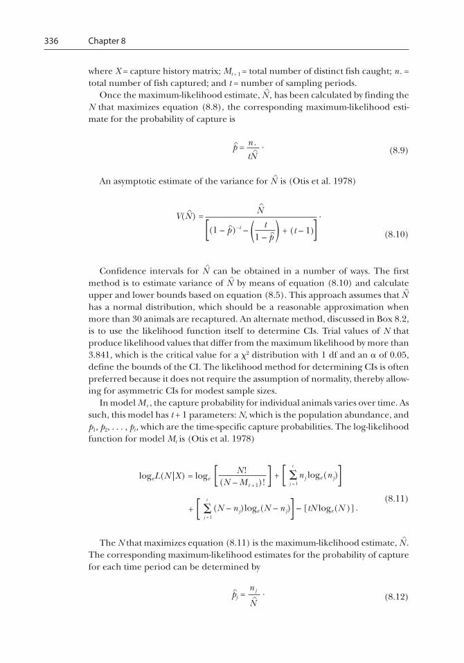
In many situations, visual observation misses some proportion of the popula-tion, even in situations where fish are constrained. Because of this, estimates ofdensity for individual sites are imprecise and contribute to the overall imprecisionof total density estimates. In order to estimate the proportion observed within asampling site, additional information needs to be gathered. The most commonlyused method is to measure the distance that each animal observed lies off thetransect (i.e., the right-angle distance from each animal seen to the transect) orfrom the center of a fixed point of observation. Depending on the observationtechnique, this distance can be determined directly, or the distance and angle ofdeparture from the transect can be determined and the right-angle distance cal-culated by simple geometry. Generally, the proportion of fish present that are
Abundance, Biomass, and Production 329
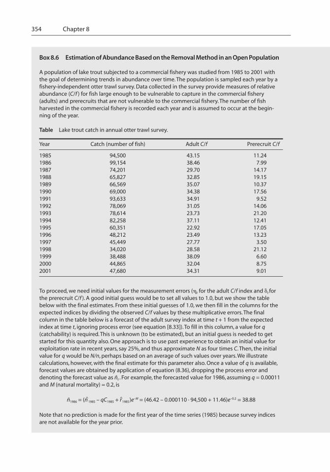
detected (i.e., sightability) declines farther from the point of observation or fromthe transect surveyed (Figure 8.1). Assuming that fish are randomly distributedwith respect to the transect and sightability is 100% at or near the center of thetransect, the proportion observed can be estimated as a function of distance fromthe transect.
Critical assumptions for applying the direct observation approach include (1)fish are randomly and independently distributed, and movement of the observerdoes not attract or repel fish prior to observation; (2) distances are measuredaccurately; (3) fish are not counted more than once; (4) fish are detected at theiroriginal position with respect to the transect; and (5) sighting of each fish is inde-pendent of other fish, meaning that the likelihood of seeing an individual fish
Figure 8.1 Example of animals sighted in a transect survey. The histogram depicts the relativefrequency of observations within 0.1-m intervals from the transect. The shaded box depicts theeffective width of the transect. Open circles indicate fish that are not sighted and closed circlesindicate fish that are sighted. Figure modified from Thompson et al. (1998).
0
1
2
3
4
5
Freq
uen
cy
0–9 10–19 20–29 30–39 40–49 50–59 60–69 70–79Distance (cm)
330 Chapter 8
does not depend on the number of other fish in the vicinity (Seber 1982; Bucklandet al. 1993; Thompson et al. 1998). Carefully implemented field techniques canhelp ensure that assumptions 1–4 are met. The assumption of independentsightings, however, depends on the behavior of fish and their schooling behaviorand patchiness. When fish are sighted in groups, but the proportion of fish sightedis constant with fish density, the precision of population estimates is generallyreduced, but the population estimate is not necessarily biased (Buckland et al.1993). In cases in which the unit of observation is a school or other aggregation ofanimals, we refer the reader to Buckland et al. (1993) for methods for appropri-ately analyzing these data. When sightability varies as a function of density orschool size, estimates of fish density are likely to be biased, and the applicability ofthis approach should be reconsidered.
For a single line-transect survey, the general formula for density is (Bucklandet al. 1993)
D = n2Lw
,^
^ (8.1)
where D^ = estimated density; n = number of fish observed; w^ = estimated effective
width of transect from center; and L = transect length.When counts are conducted from a single fixed point (point plot survey), the
area surrounding the point is observed, resulting in a circular search area. In thissituation, the general formula for density is (Buckland et al. 1993)
D = n2�w 2
,^
^ (8.2)
where w^ = estimated effective search radius.In applying these formulae, a critical component is estimating w, the effective
width of the transect or search radius from a point. Essentially w corresponds toan equivalent transect for which all fish out to w are detected and all fish beyondw are not. In order to estimate this quantity accurately, it is necessary to select afunction describing the pattern of sightability with distance. Many functions canbe used to describe the sightability function. We apply two of these functions toillustrate that the choice of sightability function matters, and we provide formulaefor estimating total population abundance from density and the total area of thestudy site in Box 8.1. Buckland et al. (1993) provide a thorough discussion ofvarious sightability functions and methods for selecting among these functions.
The variance for the density estimate (and population size) for a single transectwithin a site can be estimated approximately based on the binomial distributiondescribing observed and unobserved fish (Box 8.1), assuming that fish are ran-domly and independently distributed. When multiple transects or points are ob-served, the variance among transects should be determined based on the overallsampling design, following methods outlined in Chapter 3.
Specialized software packages are available to estimate population size basedon distance sampling (for example, the comprehensive package, DISTANCE;Thomas et al. 2001; available at http://www.ruwpa.st-and.ac.uk/distance/).
Abundance, Biomass, and Production 331
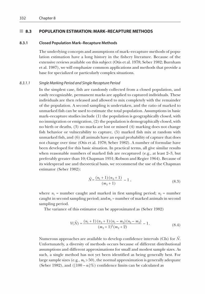
Box 8.1 Estimation of Abundance and Density Based on Distance Sampling
An investigator snorkels along a 100-m transect that is randomly located in a stream reachcontaining 500 m2. Thirty brook trout are observed at the following right-angle distances (m) fromthe center of the transect: 0.7, 0.1, 0.6, 0.3, 0.4, 0.1, 3.2, 0.4, 0.6, 1.4, 0.2, 0.1, 2.5, 0.4,4.6, 2.2, 0.5, 1.6, 0.4,0.4, 1.5, 0.8, 0.0, 0.2, 2.1, 0.4, 0.4, 0.1, 1.1, and 0.6. The investigator would like to estimate the density ofbrook trout in the section and the total population in the reach.
We define the following variables:
n = number animals observed;N = total population in reach;A = total area of reach (m2);D = density of fish (number/m2);L = length of transect (m);y = right angle distance (m) from transect for each animal;w = effective strip width;V(N
^
) = estimated variance of population estimate; andCI = confidence interval.
Based on the assumption that sightability drops off exponentially with distance from the transect,and that fish are independently distributed in the reach, we have the following (Seber 1982):
D = n
2Lw
^
^=
30
2 · 100 · 0.962= 0.156;
N = nA
2Lw
^
^=
30 · 500
2 · 100 · 0.962= 78;
w = �yn – 1
^ =27.9
30 – 1= 0.962;
V(N ) =^ n
nN^( )
2 (1 – nN^ + n
n – 2 ) = 303078
2
( )(1 – 30
78+ 30
30 – 2 ) = 342;
N ± Z �/2 V(N )^ ^
CI = = 78 ± 1.96 342 = 78 ± 36 = 42, 114.
Based on the assumption that the sightability function follows a half-normal distribution, theformula for effective width is (Buckland et al. 1993)
w = 2
��(y2/n)
^ =1
= 1.752,1
2� · 1.956
and density is calculated as above:
D = ^ 302 · 100 · 1.752
= 0.086.
If sightability drops off exponentially, the estimated population is 78 with an approximate CI of 42to 114. Note that the density (and hence total abundance) based on a half-normal distribution isapproximately half that obtained with an exponential model, highlighting the need to test theassumed sightability function (see Buckland et al. 1993 for these methods).
332 Chapter 8
■ 8.3 POPULATION ESTIMATION: MARK–RECAPTURE METHODS
8.3.1 Closed Population Mark–Recapture Methods
The underlying concepts and assumptions of mark–recapture methods of popu-lation estimation have a long history in the fishery literature. Because of theextensive reviews available on this subject (Otis et al. 1978; Seber 1982; Burnhamet al. 1987), we will emphasize common applications and methods that provide abase for specialized or particularly complex situations.
8.3.1.1 Single Marking Period and Single Recapture Period
In the simplest case, fish are randomly collected from a closed population, andeasily recognizable, permanent marks are applied to captured individuals. Theseindividuals are then released and allowed to mix completely with the remainderof the population. A second sampling is undertaken, and the ratio of marked tounmarked fish can be used to estimate the total population. Assumptions in basicmark–recapture studies include (1) the population is geographically closed, withno immigration or emigration, (2) the population is demographically closed, withno birth or deaths, (3) no marks are lost or missed (4) marking does not changefish behavior or vulnerability to capture, (5) marked fish mix at random withunmarked fish, and (6) all animals have an equal probability of capture that doesnot change over time (Otis et al. 1978; Seber 1982). A number of formulae havebeen developed for this basic situation. In practical terms, all give similar resultswhen reasonable numbers of marked fish are recaptured (e.g., at least 2–3, butpreferably greater than 10; Chapman 1951; Robson and Regier 1964). Because ofits widespread use and theoretical basis, we recommend the use of the Chapmanestimator (Seber 1982):
N = (n1 + 1)(n 2 + 1)(m 2 + 1)
– 1 ,^
(8.3)
where n1 = number caught and marked in first sampling period; n2 = numbercaught in second sampling period; andm2 = number of marked animals in secondsampling period.
The variance of this estimator can be approximated as (Seber 1982)
V(N) = (n1 + 1)(n 2 + 1)(n1 – m 2)(n2 – m 2)(m 2 + 1)2(m 2 + 2)
– 1.^
(8.4)
Numerous approaches are available to develop confidence intervals (CIs) for N^.
Unfortunately, a diversity of methods occurs because of different distributionalassumptions and different approximations for small and modest sample sizes. Assuch, a single method has not yet been identified as being generally best. Forlarge sample sizes (e.g., m2 > 50), the normal approximation is generally adequate(Seber 1982), and ([100 – �]%) confidence limits can be calculated as
Abundance, Biomass, and Production 333
N ± Z�/2 V(N). ^ ^ (8.5)
For a 95% CI, � = 0.05, and Z�/2 = 1.96. When there are fewer than 50 recaptures,Chapman (1948; reproduced in Seber 1982 and Appendix) provides a table fromwhich CIs can be calculated based on the number of recaptured fish.
8.3.1.2 The Schnabel Method
When multiple marking and recapture samples are collected over a short period(so that the population is closed with no immigration, emigration, recruitment,or mortality), population size can be estimated with the Schnabel method(Schnabel 1938; Seber 1982):
N = niMi
,^�i = 2
t
mi + 1�i = 2
t (8.6)
where t = number of sampling occasions; ni = number of fish caught in ith sample;mi = number of fish with marks caught in ith sample; and Mi = number of markedfish present in the population for ith sample.
The variance of this estimator can be approximated as (Seber 1982)
(�niMi)2
V(N) = ^ N
^
�niMi
+ 2 ·[ N 2^
(�niMi)3
+ 6 · N 3^
].N 2^
(8.7)
Confidence intervals for N^ with the Schnabel method can be computed following
the same recommendations for the Chapman method in a single mark–recaptureexperiment.
8.3.1.3 Multiple Recapture Events with Uniquely Marked Individuals
In many situations, a simple design using a single marking period and single re-capture period or a Schnabel-type design is sufficient to estimate population abun-dance. The effectiveness of such designs, however, rests on adequately meetingthe assumptions. Unfortunately, it is generally not possible to test these assump-tions using the data collected during a single recapture period or when fish aresimply marked as being previously caught. To test the assumptions underlyingmark–recapture methods of population estimation, it is generally necessary tosample over multiple periods and to have marks that allow for the capture historyof individual fish to be determined (e.g., by using individually numbered tags).
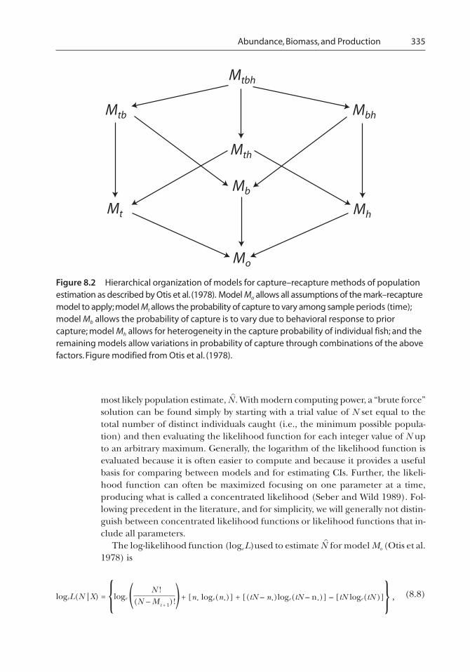
For closed populations with uniquely marked fish, Otis et al. (1978) present ahierarchical suite of models intended to cover a range of situations for whichparticular assumptions hold (Figure 8.2). The simplest, yet most restrictive, modelis that for which all assumptions listed earlier apply (Mo). In the next tier of mod-els, three basic mechanisms causing unequal capture probabilities are addressed.
334 Chapter 8
In model Mt , the probability of capture is allowed to vary among different sampleperiods (time). Variability in capture over time may occur due to factors such asweather or due to changes in the amount or type of fishing gear deployed. Inmodel Mb, the probability of capture is allowed to vary due to behavioral responseto prior capture (i.e., fish become more prone or less prone to capture after be-ing caught, handled, and marked). In surveys of small mammals, for example,investigators find that marked animals may become trap happy or trap shy, thusbiasing population estimates if such behavior is not considered (Seber 1982). Thefinal model, Mh, allows for heterogeneity in the capture probability of individualfish. This heterogenity may occur for a variety of reasons, including inherent fea-tures of each fish, such as its size, or less obvious factors such as variation in thesize of home ranges, resulting in different vulnerabilities to passive gears such astrap nets. Methods have been developed to estimate population size for each ofthese models and are illustrated below. Because of the complexity of the requiredanalyses, we strongly recommend the use of specialized software when applyingthese models. The program MARK (White and Burnham 1999; available at http://www.cnr.colostate.edu/~gwhite/mark/mark.htm.) is a very flexible software pack-age designed to analyze data from mark–recapture studies.
In the next tier of models, variations in probability of capture occur throughcombinations of two of the above factors (Figure 8.2). Thus, model Mtb representsthe case in which capture probability varies over time, as well as with the priorcapture history of an animal (behavior). Estimation methods are also available foreach of these models; however, we refer the reader to software, such as MARK,specially designed to handle such situations. Unfortunately, no method has yetbeen developed to estimate population size and account for these three sourcesof variation simultaneously (i.e., to estimate the parameters for model Mtbh).
A central concept to estimating population size by means of these models is thecapture history of an animal. Because the population is assumed to be closed, thenumber of animals in the population (N ) remains constant over all samplingperiods. As such, during each of the sampling periods (numbered 1 to t), ananimal can either be caught or not. For convenience, the capture history of allanimals observed can be recorded in a matrix in which a 1 is used to indicate acapture and 0 to indicate no capture during a particular sampling period.
The second concept central to estimating population size based on these mod-els is the likelihood function. Although this is the foundation for many methodsof population estimation (in fact, it is the basis for the Chapman and Schnabelestimators), likelihood functions may be unfamiliar to many readers. We providea brief synopsis of this topic in the context of population estimators in Box 8.2.Readers should consult texts in mathematical statistics (e.g., Bickel and Doksum1977; Rice 1995) for a more thorough treatment. In some cases, likelihood meth-ods result in a formula for directly estimating population abundance. In mostsituations, however, there is no direct formula relating the data to the populationestimate. Instead, the likelihood function is repeatedly evaluated at trial values ofN (or related parameters that determine N ) until a value of N is found that pro-duces the maximum value of the likelihood function. This is chosen as the best or
Abundance, Biomass, and Production 335
most likely population estimate, N^. With modern computing power, a “brute force”
solution can be found simply by starting with a trial value of N set equal to thetotal number of distinct individuals caught (i.e., the minimum possible popula-tion) and then evaluating the likelihood function for each integer value of N upto an arbitrary maximum. Generally, the logarithm of the likelihood function isevaluated because it is often easier to compute and because it provides a usefulbasis for comparing between models and for estimating CIs. Further, the likeli-hood function can often be maximized focusing on one parameter at a time,producing what is called a concentrated likelihood (Seber and Wild 1989). Fol-lowing precedent in the literature, and for simplicity, we will generally not distin-guish between concentrated likelihood functions or likelihood functions that in-clude all parameters.
The log-likelihood function (loge L)used to estimate N^ for model Mo (Otis et al.
1978) is
(8.8)
Figure 8.2 Hierarchical organization of models for capture–recapture methods of populationestimation as described by Otis et al. (1978). Model Mo allows all assumptions of the mark–recapturemodel to apply; model Mt allows the probability of capture to vary among sample periods (time);model Mb allows the probability of capture is to vary due to behavioral response to priorcapture; model Mh allows for heterogeneity in the capture probability of individual fish; and theremaining models allow variations in probability of capture through combinations of the abovefactors. Figure modified from Otis et al. (1978).
Mtbh
Mth
Mb
Mo
MbhMtb
Mt Mh
logeL(N |X) = {loge( N !(N – Mt + 1)!) + [n· loge(n·)] + [(tN – n·)loge(tN – n·)] – [tN loge(tN )]} ,
336 Chapter 8
where X = capture history matrix; Mt + 1 = total number of distinct fish caught; n. =total number of fish captured; and t = number of sampling periods.
Once the maximum-likelihood estimate, N^, has been calculated by finding the
N that maximizes equation (8.8), the corresponding maximum-likelihood esti-mate for the probability of capture is
p = n.
tN.^
^ (8.9)
An asymptotic estimate of the variance for N^ is (Otis et al. 1978)
V(N) = .^ N^
[(1 – p)–t –1 – p
t^
^( ) + (t – 1)] (8.10)
Confidence intervals for N^ can be obtained in a number of ways. The first
method is to estimate variance of N^ by means of equation (8.10) and calculate
upper and lower bounds based on equation (8.5). This approach assumes that N^
has a normal distribution, which should be a reasonable approximation whenmore than 30 animals are recaptured. An alternate method, discussed in Box 8.2,is to use the likelihood function itself to determine CIs. Trial values of N thatproduce likelihood values that differ from the maximum likelihood by more than3.841, which is the critical value for a �2 distribution with 1 df and an � of 0.05,define the bounds of the CI. The likelihood method for determining CIs is oftenpreferred because it does not require the assumption of normality, thereby allow-ing for asymmetric CIs for modest sample sizes.
In model Mt , the capture probability for individual animals varies over time. Assuch, this model has t + 1 parameters: N, which is the population abundance, andp1, p2, . . . , pt, which are the time-specific capture probabilities. The log-likelihoodfunction for model Mt is (Otis et al. 1978)
logeL(N |X) = loge [ N !(N – Mt + 1)! ] + [ ]�
j = 1
t
n j loge(nj)
+ [ ]�j = 1
t
(N – n j)loge(N – n j) – [tN loge(N )].(8.11)
The N that maximizes equation (8.11) is the maximum-likelihood estimate, N^.
The corresponding maximum-likelihood estimates for the probability of capturefor each time period can be determined by
pj = nj
N.^
^ (8.12)
Abundance, Biomass, and Production 337
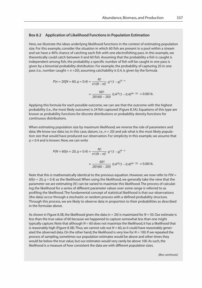
Box 8.2 Application of Likelihood Functions in Population Estimation
Here, we illustrate the ideas underlying likelihood functions in the context of estimating populationsize. For this example, consider the situation in which 60 fish are present in a pool within a streamand we have a 40% chance of catching each fish with one electrofishing pass. In this example, wetheoretically could catch between 0 and 60 fish. Assuming that the probability a fish is caught isindependent among fish, the probability a specific number of fish will be caught in one pass isgiven by a binomial probability distribution. For example, the probability of capturing 20 in onepass (i.e., number caught = n =20), assuming catchability is 0.4, is given by the formula
P(n = 20|N = 60, q = 0.4) = N !
n ! (N – n)!q n(1 – q)N – n
60!20! (60 – 20)!
0.420(1 – 0.4)60 –20= = 0.0616.
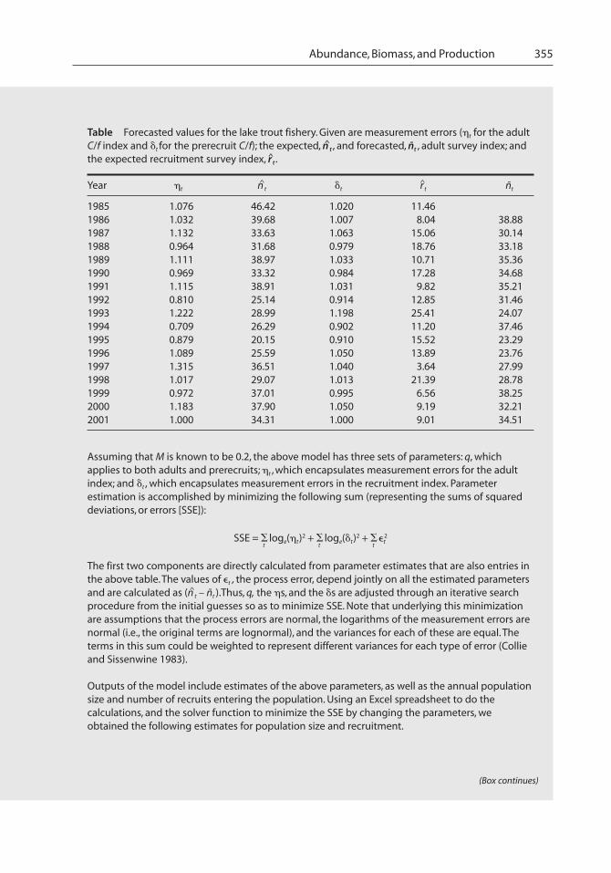
Applying this formula for each possible outcome, we can see that the outcome with the highestprobability (i.e., the most likely outcome) is 24 fish captured (Figure 8.3A). Equations of this type areknown as probability functions for discrete distributions or probability density functions forcontinuous distributions.
When estimating population size by maximum likelihood, we reverse the role of parameters anddata. We know our data (or, in this case, datum, i.e., n = 20) and ask what is the most likely popula-tion size that would have produced our observation. For simplicity in this example, we assume thatq = 0.4 and is known. Now, we can write
P(N = 60|n = 20, q = 0.4) = N !
n ! (N – n)!q n(1 – q)N – n
60!20! (60 – 20)!
0.420(1 – 0.4)60 –20= = 0.0616.
Note that this is mathematically identical to the previous equation. However, we now refer to P(N =60|n = 20, q = 0.4) as the likelihood. When using the likelihood, we generally take the view that theparameter we are estimating (N ) can be varied to maximize this likelihood. The process of calculat-ing the likelihood for a series of different parameter values over some range is referred to asprofiling the likelihood. The fundamental concept of statistical likelihood is that our observations(the data) occur through a stochastic or random process with a defined probability structure.Through this process, we are likely to observe data in proportion to their probabilities as describedin the formulae above.
As shown in Figure 8.3B, the likelihood given the data (n = 20) is maximized for N = 50. Our estimate isless than the true value of 60 because we happened to capture somewhat less than one mighttypically capture. Note that although N = 60 does not maximize the likelihood, it has a likelihood thatis reasonably high (Figure 8.3B). Thus, we cannot rule out N = 60, as it could have reasonably gener-ated the observed data. On the other hand, the likelihood is very low for N = 100. If we repeated theprocess of sampling, sometimes our population estimates would be above and other times theywould be below the true value, but our estimates would very rarely be above 100. As such, thelikelihood is a measure of how consistent the data are with different population sizes.
(Box continues)
338 Chapter 8
In this simple example, we assumed that q was known. If we had not, we could not have computeda unique solution (e.g., our data could have resulted from a combination of smaller q and larger N).As indicated in the introduction to this chapter, we generally need more information than catch perunit effort (C/f ) from a single sampling event to estimate true abundance. In our simple example,the additional information we need is the probability of capture with a single pass (i.e.,catchability).
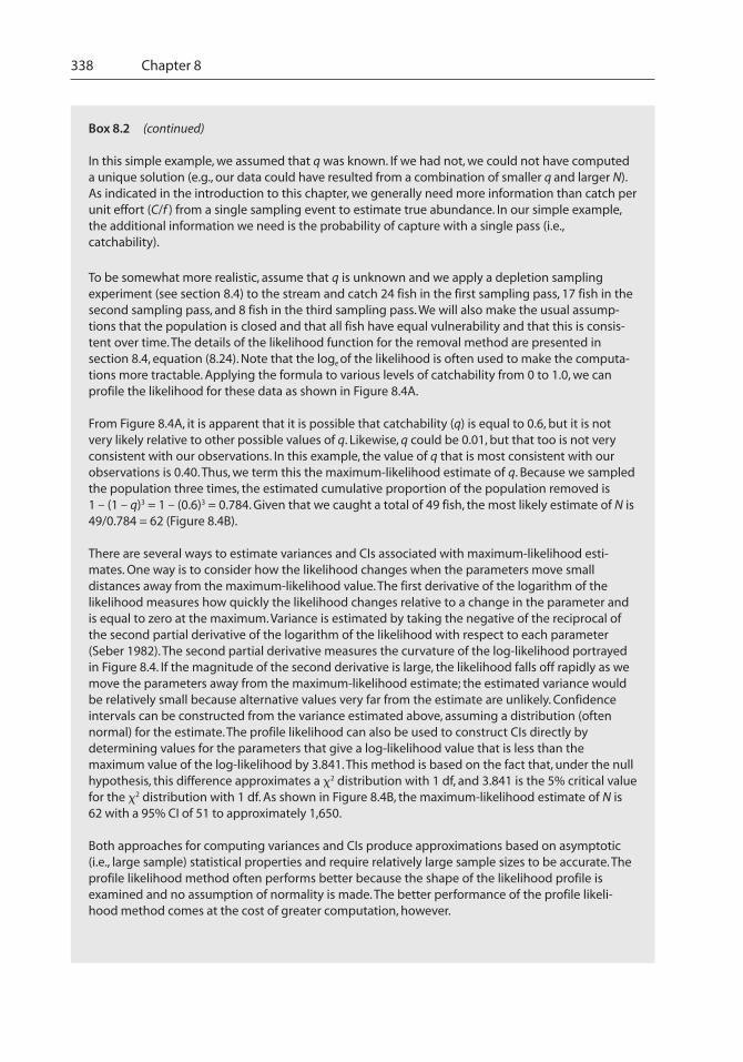
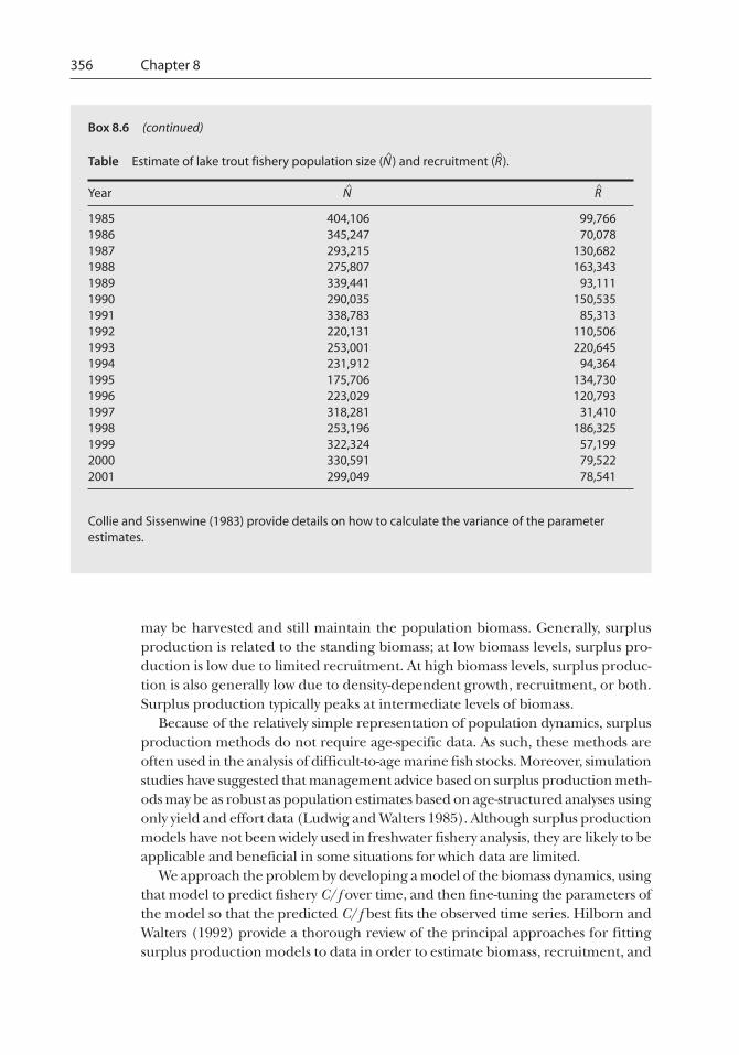
To be somewhat more realistic, assume that q is unknown and we apply a depletion samplingexperiment (see section 8.4) to the stream and catch 24 fish in the first sampling pass, 17 fish in thesecond sampling pass, and 8 fish in the third sampling pass. We will also make the usual assump-tions that the population is closed and that all fish have equal vulnerability and that this is consis-tent over time. The details of the likelihood function for the removal method are presented insection 8.4, equation (8.24). Note that the loge of the likelihood is often used to make the computa-tions more tractable. Applying the formula to various levels of catchability from 0 to 1.0, we canprofile the likelihood for these data as shown in Figure 8.4A.
From Figure 8.4A, it is apparent that it is possible that catchability (q) is equal to 0.6, but it is notvery likely relative to other possible values of q. Likewise, q could be 0.01, but that too is not veryconsistent with our observations. In this example, the value of q that is most consistent with ourobservations is 0.40. Thus, we term this the maximum-likelihood estimate of q. Because we sampledthe population three times, the estimated cumulative proportion of the population removed is1 – (1 – q)3 = 1 – (0.6)3 = 0.784. Given that we caught a total of 49 fish, the most likely estimate of N is49/0.784 = 62 (Figure 8.4B).
There are several ways to estimate variances and CIs associated with maximum-likelihood esti-mates. One way is to consider how the likelihood changes when the parameters move smalldistances away from the maximum-likelihood value. The first derivative of the logarithm of thelikelihood measures how quickly the likelihood changes relative to a change in the parameter andis equal to zero at the maximum. Variance is estimated by taking the negative of the reciprocal ofthe second partial derivative of the logarithm of the likelihood with respect to each parameter(Seber 1982). The second partial derivative measures the curvature of the log-likelihood portrayedin Figure 8.4. If the magnitude of the second derivative is large, the likelihood falls off rapidly as wemove the parameters away from the maximum-likelihood estimate; the estimated variance wouldbe relatively small because alternative values very far from the estimate are unlikely. Confidenceintervals can be constructed from the variance estimated above, assuming a distribution (oftennormal) for the estimate. The profile likelihood can also be used to construct CIs directly bydetermining values for the parameters that give a log-likelihood value that is less than themaximum value of the log-likelihood by 3.841. This method is based on the fact that, under the nullhypothesis, this difference approximates a �2 distribution with 1 df, and 3.841 is the 5% critical valuefor the �2 distribution with 1 df. As shown in Figure 8.4B, the maximum-likelihood estimate of N is62 with a 95% CI of 51 to approximately 1,650.
Both approaches for computing variances and CIs produce approximations based on asymptotic(i.e., large sample) statistical properties and require relatively large sample sizes to be accurate. Theprofile likelihood method often performs better because the shape of the likelihood profile isexamined and no assumption of normality is made. The better performance of the profile likeli-hood method comes at the cost of greater computation, however.
Box 8.2 (continued)
Abundance, Biomass, and Production 339
The asymptotic variance of N^ under model Mt is (Otis et al. 1978)
V(N) = .^ N^
(1 – p j)1 – p j
1^
^
�j = 1
t
1 + (t – 1) – � (8.13)
As with model Mo, CIs for N^ under model Mt can be estimated using the vari-
ance of N^ and an assumption of normality or through a likelihood-based approach
as outlined in Box 8.2.Model Mb (variability in capture probability due to changes in behavior after
capture) has three parameters: N, p, the probability of capturing an unmarkedanimal, and c, the probability of capturing an animal that was previously cap-tured, marked, and released. The parameter c can be estimated separately fromestimation of N and p by (Otis et al. 1978)
Figure 8.3 (A) Probability of capturing n fish from a population with 60 individuals, each witha 40% chance of capture, and (B) log-likelihood of the observation (n = 20 fish caught) as afunction of population size (N).
0.15
0.10
0.05
0.00
Pro
bab
ility
0 10 20 30 40 50 60
A
0.15
0.10
0.05
0.00
Like
liho
od
Number caught
B
0 10 20 30 40 50 60
Population size
70 80 90 100
340 Chapter 8
c = m.M.
,^(8.14)
where m· = �mj ; mj = number of marked animals in j th sample; M· = �Mj ; and Mj
= number of marked animals in the population for the j th sample.The likelihood function for model Mb is (Otis et al. 1978)
(8.15)
logeL(N) = loge[ N !(N – Mt + 1)!] + [Mt + 1 loge(Mt + 1 )]
– [(tN – M.)loge(tN – M.)] + m. loge(c ) + (M. – m.)loge(1 – c )^ ^ .
+ [(tN – M. – Mt + 1 )loge(tN – M. – Mt + 1 )]
Figure 8.4 Log-likelihood as a function of (A) catchability (q) and (B) population size (N) givendepletion sampling experiment described in Box 8.2.
–46
–47
–48
–49
–50
–51
–520 50 100 150 200 250 300 350 400
–46
–47
–48
–49
–50
–51
–520 0.2 0.4 0.6 0.8 1
Log
-like
liho
od
Log
-like
liho
od
Population size
Catchability
A
B
Abundance, Biomass, and Production 341
Once N^ has been found by maximizing equation (8.15), the maximum-likeli-
hood estimate of p is calculated as (Otis et al. 1978)
p = Mt + 1
tN – M..^
^ (8.16)
An asymptotic variance estimate for N^ is (Otis et al. 1978)
V(N) = .^ N(1 – p)t[1 – (1 – p)t]^
[1 – (1 – p)t^ ^– t 2p 2(1 – p )]^ ^
2^ t – 1
(8.17)
Estimation of the parameters for model Mh is more problematic than it is formodel Mo, Mt, or Mb. The reason for this is that each fish (including unobservedfish) has its own individual catchability. A number of approaches have been takento solve this problem, generally by making an assumption regarding the statisticaldistribution of catchabilities. For details of computation for this model, we refer thereader to Otis et al. (1978) and to the program MARK (White and Burnham 1999).
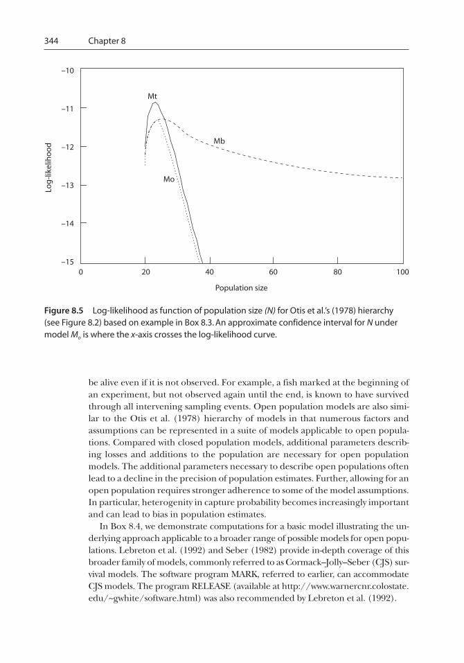
An example applying models Mo, Mt, and Mb is given in Box 8.3. Beyond beingable to estimate the parameters for each of these models, an important questionis how to choose among them. The most common way of doing this is to comparethe maximum-likelihood value for each model and select the model with the high-est maximum likelihood. Because the maximum likelihood that can be obtainedgenerally increases as more parameters are added, the likelihood obtained frommodels with more parameters is typically “penalized” for the additional flexibilityoffered. The most widely used adjustment to the likelihood function is Akaike’sInformation Criterion (AIC; Akaike 1973), which is calculated as
AIC = –2 loge(likelihood) + 2 (number of parameters). (8.18)
After computing the AIC, one then selects the model that has the lowest AICvalue (Box 8.3).
8.3.2 Open Population Mark–Recapture Methods
Open populations are characterized by having immigration, emigration, mortal-ity, or recruitment occur during the study period. As in closed populations, gen-eral models developed to estimate abundance in open populations also make useof the encounter history matrix as the basis for maximum-likelihood estimatorsand assume that each fish is uniquely marked. Conceptually, the encounter his-tory matrix is important because it defines which animals are observed at particu-lar times. From this, we can also infer which time periods the animal is known to

342 Chapter 8
Box 8.3 Estimation of Population Abundance for a Closed PopulationBased on Otis et al.’s (1978) Mark–Recapture Models
An investigator conducts a mark–recapture study on a closed population of largemouth bass in afarm pond in order to determine the abundance of adult fish. The sampling consists of foursampling events; fish captured in each event are given a uniquely numbered Floy Tag and released.The capture–recapture data are arranged into a capture matrix in which each cell of the matrix (Xij)is referenced by fishi in row i and sample periodj in column j. An entry of 1 in the matrix indicatesthat a fish was caught, and a 0 indicates that the fish was not caught during that sampling period.Fish 1, for example was caught in all four sampling periods, whereas fish 4 was caught in only thefirst sample period.
TTTTTableableableableable Data matrix for mark–recapture study of closed population of largemouth bass.
Fish Sample 1 Sample 2 Sample 3 Sample 4
1 1 1 1 12 1 1 0 03 1 0 1 04 1 0 0 05 1 1 0 16 1 0 1 17 1 0 0 08 0 1 1 09 0 1 0 010 0 1 0 111 0 1 0 012 0 1 0 013 0 1 1 114 0 0 1 015 0 0 1 016 0 0 1 017 0 0 1 118 0 0 0 119 0 0 1 120 0 0 0 1
From these data, the investigator explores which of the Otis et al. (1978) suite of capture–recapturemodels is most appropriate. For this investigation, we obtain the following basic statistics that areused in the estimation of population abundance, for which t = number of sampling occasions; ni =number of fish caught in ith sample; mi = number of fish with marks caught in ith sample; and Mi =number of marked fish present in the population for ith sample.
t = 4;Mt + 1 = 20;n1 = 7, n2 = 9, n3 = 10, n4 = 9, n . = 35;m1 = 0, m2 = 3, m3 = 5, m4 = 7, m . = 15; andM1 = 0, M2 = 7, M3 = 13, M4 = 18, M . = 38.
Abundance, Biomass, and Production 343
logeL(N = 30| X) = {loge( 30!
(30 – 20)! ) + [35loge(35)] + [(4 ·30 – 35)loge(4 ·30 – 35)] – [4 ·30loge(4 ·30)]} = –12.890; and^
logeL(N = 23| X) = {loge( 23!
(23 – 20)! ) + [35loge(35)] + [(4 ·23 – 35)loge(4 ·23 – 35)] – [4 ·23loge(4 ·23)]} = –11.299.^
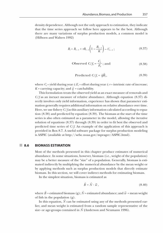
Starting with Model Mo (see Figure 8.2), we compute the log-likelihood for trial values for N^
byapplying equation (8.8). Two examples for trial values are 30 and 23. Using these values, we obtain
When the log-likelihood is computed and plotted for trial values of N^
ranging from 21 to 100 formodel Mt (equation [8.11]), we find that the maximum of the log-likelihood is
The maximum of the log-likelihood for model Mt is –10.854 at N^
= 23 (Figure 8.5).
When model Mb is employed (equation [8.15]), the log-likelihood for the same trial values is
The maximum of the log-likelihood for model Mb is –11.247 at N^
= 24 (Figure 8.5). The Akaike’sInformation Criterion (AIC) for each model is
AIC for Mo = –2(–11.299) + 2(2) = 26.598;AIC for Mt = –2(–10.854) + 2(5) = 31.708; andAIC for Mb = –2(–11.247) + 2(3) = 28.494.
Based on the AIC, we would choose model Mo as the best model among those considered. Thelikelihood for this model is not substantially lower than for Mt and Mb, but it requires fewer param-eters, resulting in a more parsimonious model.
logeL(N = 30|X) = loge [ 30!(30 – 20)! ] + [7 loge(7) + 9 loge(9) + 10 loge(10) + 9 loge(9)]
+ {[(30 – 7)loge(30 – 7)] + [(30 – 9)loge(30 – 9)] + [(30 – 10)loge(30 – 10)]
^
+ [(30 – 9)loge(30 – 9)]} – [4 ·30 loge(30)] = –12.492; and
logeL(N = 23|X) = loge [ 23!(23 – 20)! ] + [7 loge(7) + 9 loge(9) + 10 loge(10) + 9 loge(9)]
+ {[(23 – 7)loge(23 – 7)] + [(23 – 9)loge(23 – 9)] + [(23 – 10)loge(23 – 10)]
^
+ [(23 – 9)loge(23 – 9)]} – [4 ·23 loge(23)] = –10.854.
logeL(30|X) = loge [ 30!(30 – 20)! ] + [20loge(20)] + [(4 ·30 – 38 – 20)loge(4 ·30 – 38 – 20)]
– [(4 ·30 – 38)loge(4 ·30 – 38)] + 15loge(0.395) + (38 – 15) loge(1 – 0.395)] = –11.491; and
logeL(23|X) = loge [ 23!(23 – 20)! ] + [20loge(20)] + [(4 ·23 – 38 – 20)loge(4 ·23 – 38 – 20)]
– [(4 ·23 – 38)loge(4 ·23 – 38)] + 15loge(0.395) + (38 – 15) loge(1 – 0.395)] = –11.270.
344 Chapter 8
be alive even if it is not observed. For example, a fish marked at the beginning ofan experiment, but not observed again until the end, is known to have survivedthrough all intervening sampling events. Open population models are also simi-lar to the Otis et al. (1978) hierarchy of models in that numerous factors andassumptions can be represented in a suite of models applicable to open popula-tions. Compared with closed population models, additional parameters describ-ing losses and additions to the population are necessary for open populationmodels. The additional parameters necessary to describe open populations oftenlead to a decline in the precision of population estimates. Further, allowing for anopen population requires stronger adherence to some of the model assumptions.In particular, heterogenity in capture probability becomes increasingly importantand can lead to bias in population estimates.
In Box 8.4, we demonstrate computations for a basic model illustrating the un-derlying approach applicable to a broader range of possible models for open popu-lations. Lebreton et al. (1992) and Seber (1982) provide in-depth coverage of thisbroader family of models, commonly referred to as Cormack–Jolly–Seber (CJS) sur-vival models. The software program MARK, referred to earlier, can accommodateCJS models. The program RELEASE (available at http://www.warnercnr.colostate.edu/~gwhite/software.html) was also recommended by Lebreton et al. (1992).
Figure 8.5 Log-likelihood as function of population size (N) for Otis et al.’s (1978) hierarchy(see Figure 8.2) based on example in Box 8.3. An approximate confidence interval for N undermodel Mo is where the x-axis crosses the log-likelihood curve.
–10
–11
–12
–13
–14
–15
Log
-like
liho
od
0 20 40 60 80 100
Population size
Mt
Mb
Mo
Abundance, Biomass, and Production 345
Box 8.4 represents a commonly used open population model in which theabundance of animals changes over time due to births and deaths, survival variesover time, but capture probability is constant over time and across all individualsin the population. As such, this model is analogous to model Mo, with the additionof time-varying population abundance and survival. In the CJS models, four basicsets of parameters are estimated: population abundance (Ni), capture probability(pi), apparent survival (�i), and additions (births and immigrant) to the popula-tion (Bi). The term apparent survival is used instead of survival because, in mostcases, it is impossible to distinguish any losses due to emigration from mortality. Ifthe population is geographically closed, �i is an estimator for actual survival rate.Each of the above parameters are indexed by time, but care must be taken inunderstanding that �i indicates the survival rate from time i to i + 1. Further, notall quantities are estimable; for example, abundance at the beginning of the study(N1) generally cannot be determined. The application of this model is illustratedin Box 8.4. For simple models, closed-form equations exist to estimate populationsize and other necessary parameters. In more complex situations, an iterative (i.e.,starting with an initial guess, and then using a numerical optimization to improvethe fit) approach is necessary to solve the likelihood equations.
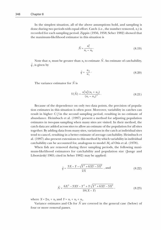
■ 8.4 POPULATION ESTIMATION: REMOVAL METHODS
8.4.1 Closed Population Removal Methods
Like mark–recapture methods, removal methods rely on sequentially samplingthe target population. During each sampling period, the number of fish capturedare recorded, and captured fish are temporarily (e.g., during monitoring surveys)or permanently (e.g., in recreational or commercial fisheries) removed from thepopulation. Through the reduction in the population, catch in subsequent sam-pling periods is reduced. The rate at which catch declines gives a measure of theproportion of the original population that has been removed.
As with mark–recapture methods, removal methods generally rely on the popu-lation being closed and individuals in the population having equal vulnerabilityto the sampling gear. Typically, equal amounts of effort are expended during eachsampling period, and it is assumed that the capture probability is equal across allsampling periods. Historically, regressions relating C/f to cumulative catch (Lesliemethod, Leslie and Davis 1939) or cumulative effort (De Lury method, De Lury1947) were used to estimate population size in removal experiments. These meth-ods are still commonly used and often result in reasonable population estimates.Currently, there is a shift away from the regression-based methods to likelihood-based methods. The principal advantage of likelihood methods over regressionmethods is that they provide means for testing some of the assumptions of theremoval method and creating models that can accommodate a relaxed set of as-sumptions. For example, the assumption of equal catchability over all samplingperiods can be relaxed if a function can be used to describe how catchabilitychanges over time.

346 Chapter 8
Box 8.4 Estimation of Abundance Based on a Cormack–Jolly–Seber Modelfor Open Populations
In order to determine the conservation status of desert pupfish, a graduate student performs a3-year capture–recapture experiment on the population in a desert pool that is closed to immigra-tion and emigration but where recruitment and mortality occur on an annual basis.
Table Capture matrix from capture–recapture experiment with desert pupfish.
Year
Fish idenfication 1998 1999 2000
1 1 1 12 1 1 13 1 1 04 1 1 05 1 0 16 1 0 17 1 0 18 1 0 19 1 0 010 1 0 011 1 0 012 1 0 013 1 0 014 0 1 115 0 1 116 0 1 117 0 1 118 0 1 019 0 1 020 0 1 021 0 1 022 0 0 123 0 0 124 0 0 125 0 0 126 0 0 127 0 0 128 0 0 129 0 0 130 0 0 1
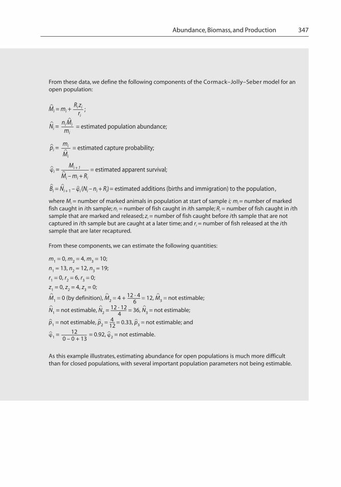
Abundance, Biomass, and Production 347
m1 = 0, m2 = 4, m3 = 10;
n1 = 13, n2 = 12, n3 = 19;
r1 = 0, r2 = 6, r3 = 0;
z1 = 0, z2 = 4, z3 = 0;
M1 = 0 (by definition), M2 = 4 + 12 · 4 = 12, M3 = not estimable;
N1 = not estimable, N2 = 12 · 12 = 36, N3 = not estimable;
p1 = not estimable, p2 = 4 = 0.33, p3 = not estimable; and
�1 = 12 = 0.92, �2 = not estimable.
6^^ ^
^^ ^
4
12^^ ^
0 – 0 + 13^^
Ni = ni Mi
mi
^^
= estimated population abundance;
Mi = mi + Ri zi
ri
^;
pi = mi
Mi
^ = estimated capture probability;^
�i = Mi + 1
Mi – mi + Ri
^ = estimated apparent survival;^
Bi = Ni + 1 – �i (Ni – ni + Ri) = estimated additions (births and immigration) to the population,^ ^ ^
From these data, we define the following components of the Cormack–Jolly–Seber model for anopen population:
where Mi = number of marked animals in population at start of sample i; mi = number of markedfish caught in ith sample; ni = number of fish caught in ith sample; Ri = number of fish caught in ithsample that are marked and released; zi = number of fish caught before ith sample that are notcaptured in ith sample but are caught at a later time; and ri = number of fish released at the ithsample that are later recaptured.
From these components, we can estimate the following quantities:
As this example illustrates, estimating abundance for open populations is much more difficultthan for closed populations, with several important population parameters not being estimable.
348 Chapter 8
In the simplest situation, all of the above assumptions hold, and sampling isdone during two periods with equal effort. Catch (i.e., the number removed, ni) isrecorded for each sampling period. Zippin (1956, 1958; Seber 1982) showed thatthe maximum-likelihood estimator in this situation is
N = n1
n1 – n2
.^2
(8.19)
Note that n1 must be greater than n2 to estimate N^. An estimate of catchability,
q^, is given by
q = n 2
n 1
.^ (8.20)
The variance estimator for N^ is
V(N) = n1
2n22(n1 + n 2)
(n1 – n 2)4
.^
(8.21)
Because of the dependence on only two data points, the precision of popula-tion estimates in this situation is often poor. Moreover, variability in catches canresult in higher C/f in the second sampling period, resulting in no estimate ofabundance. Heimbuch et al. (1997) present a method for adjusting populationestimates in two-pass sampling when many sites are visited. In their method, thecatch data are added across sites to allow an estimate of the population for all sitestogether. By adding data from many sites, variations in the catch at individual sitestend to cancel, resulting in a better estimate of average catchability. Heimbuch etal. (1997) also present extensions to this method by which variability in individualcatchability can be accounted for, analogous to model Mh of Otis et al. (1978).
When fish are removed during three sampling periods, the following maxi-mum-likelihood estimators for catchability and population size (Junge andLibosvárský 1965; cited in Seber 1982) may be applied:
q = 3X – Y – Y 2 + 6XY – 3X 2, and^
2X(8.22)
N = 6X 2 – 3XY – Y 2 + Y Y 2 + 6XY – 3X 2,^
18(X – Y)(8.23)
where X = 2n1 + n2 and Y = n1 + n2 + n3.Variance estimates and CIs for N
^ are covered in the general case (below) of
four or more removal passes.

Abundance, Biomass, and Production 349
When more than three removal passes are conducted, there is no closed-formequation available for directly estimating population size from the data by meansof current maximum-likelihood methods. As in the more complex mark–recap-ture situations, the relative likelihood of parameter values is calculated, and nu-merical search methods are used to determine which combination of parametervalues is most likely given the observed data. When catchability (q) is assumed tobe constant over time, the results of this analysis are easy to portray graphically asa profile likelihood (see Box 8.2). In the maximum-likelihood approach,catchability is generally estimated directly, and N
^ is calculated from the cumula-
tive catch and estimated cumulative proportion of the population that this repre-sents, based on the estimated catchability (Box 8.5). The likelihood function (drop-ping those parts of the function that are constants not affecting estimation) forestimating q^ is (Gould and Pollock 1997)
(8.24)
where t = number of removal passes; ni = catch in ith sample; xi = cumulative catchprior to removal pass i; qi = probability of capture in ith removal pass; and pi = 1 – qi .
Once qi has been estimated, N^ is estimated by
N = xt + 1
(1 – q t ).^
^ (8.25)
When the cumulative removal is relatively large (e.g., greater than 30), theasymptotic variance of q^ and N
^ are (Seber 1982)
V(N) = , and ^ N(1 – q t)q t^
(1 – q t)2 – {[t(1 – q)]2q t – 1^
^ ^
^ ^
(8.26)
V(q) = .^ [(1 – q)q]2(1 – q t)
N <q (1 – q t)2 – {[t(1 – q)]2q t}>^
^ ^
^^
^
^ ^
(8.27)
loge(q |n1, n2, n3, . . . nt) = loge ( xt + 1!n1!, n2!, n3!, . . . nt !)
+ n1loge ( q1
1 – q1 – p1p2 – p1p2q3 – . . . p1p2 . . . qt)
+ n2loge ( q2p1
1 – q1 – p1p2 – p1p2q3 – . . . p1p2 . . . qt)
+ n3loge ( q3p2p1
1 – q1 – p1p2 – p1p2q3 – . . . p1p2 . . . qt) + . . . ,
350 Chapter 8
Box 8.5 Estimation of Abundance Based on the Removal Method in a Closed Population
In order to estimate the abundance of brown trout in a 50-m section of stream below a culvert, afishery manager conducts a three-pass removal experiment. Fish cannot move upstream becauseof the culvert, and the manager places a block net on the lower section of the study reach to insurethat the population is geographically closed. All three sampling passes are conducted during thesame day by means of a backpack electrofishing unit. During sampling, 24 brown trout are caughtin the first sampling pass, 17 in the second sampling pass, and 8 in the third sampling pass.
Although the population size can be estimated applying equation (8.23), we illustrate the applica-tion of the more general likelihood equation (8.24). Given a trial value for catchability (q) of 0.2,
A search across a range of q^ from 0.01 to 0.99 in steps of 0.01 indicates that the most likely value ofq^ is 0.40, with a log-likelihood value of –49.832. From this, N
^ is calculated as
N = 49
(1 – 0.43) = 63,
^
with an estimated variance of
Var(N ) = ^ 63(1 – 0.4)3(0.43)
[(1 – 0.43)2] – {[3(1 – 0.4)]2(0.42)}= 10.55.
Confidence intervals are typically obtained from the profile likelihood of q^. From the search acrossvalues of q^ ranging from 0.01 to 0.99 (in 0.01 increments), the log-likelihood values for q = 0.65 andq = 0.01 differed from the log-likelihood at q^ = 0.4 by 3.841 or more (which is the critical value forthe �2 distribution with 1 df ). The population sizes corresponding to these values of q are 51 and1,650 and represent approximate 95% CIs for N
^.
loge(q = 0.2|n1 = 24, n2 = 17, n3 = 8) = loge ( 49!24!17!8! ) + 24loge ( 0.2
1 – 0.2 – (0.8)(0.2) – (0.8)(0.8)(0.2) – (0.8)(0.8)(0.8)(0.2) )+ 17loge ( (0.2)(0.8)
1 – 0.2 – (0.8)(0.2) – (0.8)(0.8)(0.2) – (0.8)(0.8)(0.8)(0.2) )+ 8loge ( (0.2)(0.8)(0.8)
1 – 0.2 – (0.8)(0.2) – (0.8)(0.8)(0.2) – (0.8)(0.8)(0.8)(0.2) ) = 60.409.
Confidence intervals can be obtained by assuming that q^ and N^ are normally
distributed (equation [8.5]) or from the profile likelihood of (e.g., Box 8.2).Once q^ and N
^ have been estimated, the goodness of fit of the estimates can be
assessed by comparing the expected catches with the observed catches. Expectedcatch for each removal pass is predicted by
�~1 = N^
q^; (8.28)
�~2 = N^
q^(1 – q^); (8.29)
Abundance, Biomass, and Production 351
�~3 = N^
q^(1 – q^)2 . . . ; and (8.30)
�~t = N^
q^(1 – q^)t – 1. (8.31)
Goodness of fit can then be assessed by a �2 test by comparing the observedcatches with the expected catches. This provides a useful diagnostic test to deter-mine if the assumption of constant catchability over time is reasonable.
�2 = �(�
i – �
i)2~
�i
~ , (8.32)
where �i = observed catch in pass i, and �~i = expected catch in pass i.One of the more common violations of the assumptions in the removal method
is that individual fish often differ in their catchability, analogous to model Mh formark–recapture studies. Two approaches can be used to estimate population sizein this situation. The first approach rests on the observation that removal studiescan be viewed as a special case of mark–recapture model Mb, where the “response”to capture is removal from the vulnerable population (this is equivalent to settingc in model Mb equal to 1.0). Heterogeneity in individual catchability can then beaccounted for by fitting model Mbh in the Otis et al. (1978) hierarchy. The calcula-tions for this model are complex, but program MARK includes this option.
The second approach for handling variations in catchability is to fit a time-varying function to q^. Because fish with higher catchability tend to be capturedand removed earlier in the sampling process, the average catchability of the re-maining population tends to decline as the population is depleted. Thus, addi-tional parameters describing how q^ declines with each sampling pass can be esti-mated. We refer the reader to Schnute (1983) for more detailed description ofthis approach.
Several software packages are available to estimate abundance from removalexperiments. White and Burnham’s (1999) MARK handles removal data well andhas the option of fitting alternate models as described above. Van Deventer andPlatts’ (1989) MicroFish is a software package available through the AmericanFisheries Society that is designed for removal studies. Its particular strength is thatremoval experiments from multiple sites and multiple species can be analyzedfrom a single data file.
8.4.2 Open Population Removal Methods
The application of removal methods to open populations is much more difficultthan it is for closed populations because mortality and recruitment need to beestimated in addition to population size. Furthermore, removal methods are gen-erally applied to open populations only when there is a fishery harvesting a sub-stantial portion of the population. As such, the timing and magnitude of removalsare often out of the fisheries scientist’s control. Further, there is the potential
352 Chapter 8
problem of under (or over) reporting of catch, resulting in biased estimates ofpopulation size. This is not to dissuade readers from pursuing removal methodsfor open populations—this is often the only feasible approach given the dataavailable. Rather, we emphasize that the particular details of the data and thefishery will determine which model is most appropriate. In this chapter, we presenta relatively simple formulation requiring minimal data to illustrate the essence ofthese methods.
Consider a population that is closed to immigration and emigration but is opento natural mortality (M), fishery harvest (C), and recruitment (R). One represen-tation of the dynamics of the population is (Collie and Sissenwine 1983)
Nt + 1 = (Nt – Ct + Rt )e–M + Et . (8.33)
In this model, Et represents random variations in mortality that are not in-cluded in either catch or natural mortality (which is assumed to be constant). Theparameter Et reflects what is often called a process error, meaning the unaccountedvariation in the underlying dynamical processes. Including this in the populationdynamic equation (8.33) is important because process error actually influencessystem dynamics, and these process errors can accumulate over time. This modelimplicitly assumes that recruitment and fishery removals occur at the beginningof the year. Natural mortality operates at a constant rate for the remainder of theyear, and a proportion (e –M) survive to the beginning of the next year. Alternativeformulations can be derived for populations for which the fishery and recruit-ment occur throughout the year (see Ricker 1977).
For the model described above, information on harvest alone is insufficient toestimate population abundance. Additional information in the form of relativeabundance indices (e.g., C/f) for the adult stock (nt ) and recruits (rt ) are alsorequired. Age-structured measures of C/f and population dynamic equations canalso be used, leading to methods such as virtual population analysis or statisticalcatch-at-age. We refer the reader to Ricker (1977), Edwards and Megrey (1989),and Hilborn and Walters (1992) for a detailed discussion of these extensions.
If we assume that the expected C/f for adults and recruits is directly propor-tional to the true population size (Nt and Rt ) and that all members of the popula-tion are equally vulnerable to the survey gear, we have
nt = n^t�t = qNt�t , and (8.34)
rt = r^t �t = qRt �t . (8.35)
where q = proportionality constant relating survey C/f to true abundance (i.e.,catchability in survey); �t = measurement error term for adults with a mean of 1.0;and �t = measurement error term for recruits with a mean of 1.0.
We have assumed that adults and recruits have equal vulnerability to the surveygear. This assumption or a known ratio of recruit to adult vulnerability is generallyrequired when using these Collie–Sissenwine catch survey models (Mesnil 2003).
Abundance, Biomass, and Production 353
A critical concept underlying equations (8.34) and (8.35) is that C/f, which isbased on samples from the entire population, is generally estimated with consid-erable variance. The variance associated with these estimates is often termedmeasurement error and, in the context of population modeling, implies that C/fshould not be treated as an exact measure of relative abundance but rather needsto be treated as being imprecise. Using equations (8.34) and (8.35) leads to thefollowing dynamic equation describing the trajectory of the expected value foradult C/f:
n^t + 1 = (n^t – qCt + r^t)e–M + �t . (8.36)
Here, �t = qEt and is the process error as it influences adult C/f. The estimationprocedure attempts to minimize these process errors as well as the measurementerrors (see Box 8.6).
Generally, M is assumed to be known and constant over time. Under the addi-tional assumption that the measurement errors are negligible (i.e., all are close to1.0), equation (8.36) can be rewritten in a form by which standard linear regres-sion can be used to estimate q (and thereby Nt and Rt ). However, as Collie andSissenwine (1983) state, nt and rt are generally both measured with substantialimprecision. Because of this, we recommend the methods of Collie and Sissenwine(1983; illustrated in Box 8.6) over a regression approach because the assumptionof negligible measurement error is rarely credible.
We are not aware of any software program that handles the broad range ofsituations that are likely to occur when using removal methods in open popula-tions. As such, practitioners must either use specialized software previously devel-oped for special cases similar to theirs or develop the models and associated es-timation routines in a general programming environment (e.g., C++, Visual Basic,or SAS), a spreadsheet environment (e.g., Microsoft Excel), or a specialized pro-gramming environment designed for statistical parameter estimation (e.g., AdModelBuilder [Otter Research, Sidney, British Columbia]). Schnute et al. (1998) discusssome of the trade-offs faced in choosing software for such modeling.
■ 8.5 BIOMASS AND YIELD ESTIMATION: SURPLUS PRODUCTION METHODS
In situations where a geographically closed population is subjected to a signifi-cant fishery (e.g., where the population has been substantially reduced by fishing;Hilborn and Walters 1992), it is sometimes possible to estimate biomass from thepattern of yield (biomass of fish removed) and fishing effort over time. Conceptu-ally, surplus production models (also known as biomass dynamic models, Hilbornand Walters 1992) are based on the idea that the biomass in a given year (Bt)depends on the biomass in the previous year (Bt – 1) plus recruitment and growthminus yield and natural mortality. It is often convenient to group recruitment andgrowth into a single term representing processes that contribute to biomass. Ifthis production is in excess of natural mortality, the surplus production will in-crease the biomass from one year to the next. Alternately, the surplus production
354 Chapter 8
Box 8.6 Estimation of Abundance Based on the Removal Method in an Open Population
A population of lake trout subjected to a commercial fishery was studied from 1985 to 2001 withthe goal of determining trends in abundance over time. The population is sampled each year by afishery-independent otter trawl survey. Data collected in the survey provide measures of relativeabundance (C/f ) for fish large enough to be vulnerable to capture in the commercial fishery(adults) and prerecruits that are not vulnerable to the commercial fishery. The number of fishharvested in the commercial fishery is recorded each year and is assumed to occur at the begin-ning of the year.
Table Lake trout catch in annual otter trawl survey.
Year Catch (number of fish) Adult C/f Prerecruit C/f
1985 94,500 43.15 11.241986 99,154 38.46 7.991987 74,201 29.70 14.171988 65,827 32.85 19.151989 66,569 35.07 10.371990 69,000 34.38 17.561991 93,633 34.91 9.521992 78,069 31.05 14.061993 78,614 23.73 21.201994 82,258 37.11 12.411995 60,351 22.92 17.051996 48,212 23.49 13.231997 45,449 27.77 3.501998 34,020 28.58 21.121999 38,488 38.09 6.602000 44,865 32.04 8.752001 47,680 34.31 9.01
To proceed, we need initial values for the measurement errors (�t for the adult C/f index and �t forthe prerecruit C/f ). A good initial guess would be to set all values to 1.0, but we show the tablebelow with the final estimates. From these initial guesses of 1.0, we then fill in the columns for theexpected indices by dividing the observed C/f values by these multiplicative errors. The finalcolumn in the table below is a forecast of the adult survey index at time t + 1 from the expectedindex at time t, ignoring process error (see equation [8.33]). To fill in this column, a value for q(catchability) is required. This is unknown (to be estimated), but an initial guess is needed to getstarted for this quantity also. One approach is to use past experience to obtain an initial value forexploitation rate in recent years, say 25%, and thus approximate N as four times C. Then, the initialvalue for q would be N/n, perhaps based on an average of such values over years. We illustratecalculations, however, with the final estimate for this parameter also. Once a value of q is available,forecast values are obtained by application of equation (8.36), dropping the process error anddenoting the forecast value as ñt . For example, the forecasted value for 1986, assuming q = 0.00011and M (natural mortality) = 0.2, is
ñ1986 = (n^1985 – qC1985 + r^1985)e–M = (46.42 – 0.000110 · 94,500 + 11.46)e–0.2 = 38.88
Note that no prediction is made for the first year of the time series (1985) because survey indicesare not available for the year prior.
Abundance, Biomass, and Production 355
Table Forecasted values for the lake trout fishery. Given are measurement errors (�t for the adultC/f index and �t for the prerecruit C/f); the expected, n^t , and forecasted, ñt , adult survey index; andthe expected recruitment survey index, r^t .
Year �t n^t �t r^t ñt
1985 1.076 46.42 1.020 11.461986 1.032 39.68 1.007 8.04 38.881987 1.132 33.63 1.063 15.06 30.141988 0.964 31.68 0.979 18.76 33.181989 1.111 38.97 1.033 10.71 35.361990 0.969 33.32 0.984 17.28 34.681991 1.115 38.91 1.031 9.82 35.211992 0.810 25.14 0.914 12.85 31.461993 1.222 28.99 1.198 25.41 24.071994 0.709 26.29 0.902 11.20 37.461995 0.879 20.15 0.910 15.52 23.291996 1.089 25.59 1.050 13.89 23.761997 1.315 36.51 1.040 3.64 27.991998 1.017 29.07 1.013 21.39 28.781999 0.972 37.01 0.995 6.56 38.252000 1.183 37.90 1.050 9.19 32.212001 1.000 34.31 1.000 9.01 34.51
Assuming that M is known to be 0.2, the above model has three sets of parameters: q, whichapplies to both adults and prerecruits; �t , which encapsulates measurement errors for the adultindex; and �t , which encapsulates measurement errors in the recruitment index. Parameterestimation is accomplished by minimizing the following sum (representing the sums of squareddeviations, or errors [SSE]):
SSE = �t
loge(�t)2 + �t
loge(�t)2 + �t
�t2
The first two components are directly calculated from parameter estimates that are also entries inthe above table. The values of �t , the process error, depend jointly on all the estimated parametersand are calculated as (n^t – ñt ).Thus, q, the �s, and the �s are adjusted through an iterative searchprocedure from the initial guesses so as to minimize SSE. Note that underlying this minimizationare assumptions that the process errors are normal, the logarithms of the measurement errors arenormal (i.e., the original terms are lognormal), and the variances for each of these are equal. Theterms in this sum could be weighted to represent different variances for each type of error (Collieand Sissenwine 1983).
Outputs of the model include estimates of the above parameters, as well as the annual populationsize and number of recruits entering the population. Using an Excel spreadsheet to do thecalculations, and the solver function to minimize the SSE by changing the parameters, weobtained the following estimates for population size and recruitment.
(Box continues)
356 Chapter 8
may be harvested and still maintain the population biomass. Generally, surplusproduction is related to the standing biomass; at low biomass levels, surplus pro-duction is low due to limited recruitment. At high biomass levels, surplus produc-tion is also generally low due to density-dependent growth, recruitment, or both.Surplus production typically peaks at intermediate levels of biomass.
Because of the relatively simple representation of population dynamics, surplusproduction methods do not require age-specific data. As such, these methods areoften used in the analysis of difficult-to-age marine fish stocks. Moreover, simulationstudies have suggested that management advice based on surplus production meth-ods may be as robust as population estimates based on age-structured analyses usingonly yield and effort data (Ludwig and Walters 1985). Although surplus productionmodels have not been widely used in freshwater fishery analysis, they are likely to beapplicable and beneficial in some situations for which data are limited.
We approach the problem by developing a model of the biomass dynamics, usingthat model to predict fishery C/f over time, and then fine-tuning the parameters ofthe model so that the predicted C/f best fits the observed time series. Hilborn andWalters (1992) provide a thorough review of the principal approaches for fittingsurplus production models to data in order to estimate biomass, recruitment, and
Box 8.6 (continued)
Table Estimate of lake trout fishery population size (N^
) and recruitment (R^
).
Year N^
R^
1985 404,106 99,7661986 345,247 70,0781987 293,215 130,6821988 275,807 163,3431989 339,441 93,1111990 290,035 150,5351991 338,783 85,3131992 220,131 110,5061993 253,001 220,6451994 231,912 94,3641995 175,706 134,7301996 223,029 120,7931997 318,281 31,4101998 253,196 186,3251999 322,324 57,1992000 330,591 79,5222001 299,049 78,541
Collie and Sissenwine (1983) provide details on how to calculate the variance of the parameterestimates.
Abundance, Biomass, and Production 357
density dependence. Although not the only approach to estimation, they indicatethat the time series approach we follow here appears to be the best. Althoughthere are many variations of surplus production models, a common model is(Hilborn and Walters 1992)
Bt = Bt – 1 + rBt – 1(1 – K
Bt – 1 ) – Ct – 1 ; (8.37)
Et
Ct ; andObserved C/ft = (8.38)
Predicted C/ft = qBt ,^^ (8.39)
where Ct = yield during year t; Et = effort during year t; r = intrinsic rate of increase;K = carrying capacity; and q^ = catchability.
This formulation treats the observed yield as an exact measure of removals andC/f as an inexact measure of relative abundance. Although equation (8.37) di-rectly involves only yield information, experience has shown that parameter esti-mation generally requires additional information on relative abundance over time.Here, we use fishery C/f as this auxiliary information calculated according to equa-tion (8.38) and predicted by equation (8.39). The biomass at the start of the timeseries is also often estimated as a parameter in the model, allowing the iterativesolution of equations (8.37) through (8.39) in order to fit best the observed andpredicted time series of C/f. An example of the application of this approach isprovided in Box 8.7. A useful software package for surplus production modelingis ASPIC (available at http://sefsc.noaa.gov/mprager/ASPIC.html).
■ 8.6 BIOMASS ESTIMATION
Most of the methods presented in this chapter produce estimates of numericalabundance. In some situations, however, biomass (i.e., weight of the population)may be a better measure of the “size” of a population. Generally, biomass is esti-mated indirectly by multiplying the numerical abundance by the mean weight orby applying methods such as surplus production models that directly estimatebiomass. In this section, we will cover indirect methods for estimating biomass.
In the simplest situation, biomass is estimated as
B^ = N
^ · w– , (8.40)
where B^ = estimated biomass (g); N
^ = estimated abundance; and w– = mean weight
of fish in the population (g).In this equation, N
^ can be estimated using any of the methods presented ear-
lier, and mean weight is estimated from a random sample representative of thesize- or age-groups contained in N
^ (Anderson and Neumann 1996).
358 Chapter 8
Box 8.7 Application of Surplus Production Modeling
The commercial fishery for a population of alewife was monitored from 1985 to 2001. Each year, thetotal weight of the catch (kg) and the total effort (days fished) were recorded, providing C/f as ameasure of relative abundance. These data were analyzed using a surplus production model toestimate carrying capacity (K), initial biomass (B0), catchability (q), and the intrinsic rate of growth (r)for this fishery population.
Table Catch and effort data for alewife fishery.
Year Effort (days fished) Catch (kg) C/f (kg/d)
1985 825 90,000 1091986 1,008 113,300 1121987 1,411 155,860 1101988 1,828 181,128 991989 2,351 198,584 841990 2,074 198,395 961991 1,877 139,040 741992 1,566 109,969 701993 1,139 71,896 631994 893 59,314 661995 1,029 62,300 611996 727 65,343 901997 658 76,990 1171998 953 88,606 931999 1,012 118,016 1172000 1,203 108,250 902001 1,034 108,674 105
With B0 = 800,000 kg, K = 4,000,000, q = 0.0001, and r = 0.17 as initial guesses for the parameters ofequations (8.37) and (8.39), we can predict catch and C/f as follows:
B1986 = B1985 + rB1985^ B1985
K– C1985
^ ^ (1 – )^
^
= 800,000 + 0.17 · 800,000 800,0004,000,000(1 – ) – 90,000 = 818,800
C/f1986 = qB1986 = 0.0001 · 818,800 = 81.88 ~ 82^ ^
~
Table Recursive application of equations (8.37) and (8.39) result in time series of predicted valuesfor the alewife fishery.
Predicted Predicted SquaredYear biomass (kg) C/f (kg/d) C/f (kg/d) deviation for C/f
1985 800,000 109 80 8411986 818,800 112 82 9611987 816,203 110 82 8411988 770,784 99 77 4841989 695,440 84 70 2251990 594,526 96 59 1369
Abundance, Biomass, and Production 359
Predicted Predicted SquaredYear biomass (kg) C/f (kg/d) C/f (kg/d) deviation for C/f
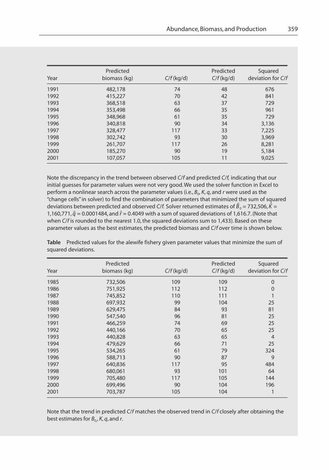
1991 482,178 74 48 6761992 415,227 70 42 8411993 368,518 63 37 7291994 353,498 66 35 9611995 348,968 61 35 7291996 340,818 90 34 3,1361997 328,477 117 33 7,2251998 302,742 93 30 3,9691999 261,707 117 26 8,2812000 185,270 90 19 5,1842001 107,057 105 11 9,025
Note the discrepancy in the trend between observed C/f and predicted C/f, indicating that ourinitial guesses for parameter values were not very good. We used the solver function in Excel toperform a nonlinear search across the parameter values (i.e., B0, K, q, and r were used as the“change cells” in solver) to find the combination of parameters that minimized the sum of squareddeviations between predicted and observed C/f. Solver returned estimates of B
^
0 = 732,506, K^
=1,160,771, q^ = 0.0001484, and r ̂= 0.4049 with a sum of squared deviations of 1,616.7. (Note thatwhen C/f is rounded to the nearest 1.0, the squared deviations sum to 1,433). Based on theseparameter values as the best estimates, the predicted biomass and C/f over time is shown below.
Table Predicted values for the alewife fishery given parameter values that minimize the sum ofsquared deviations.
Predicted Predicted SquaredYear biomass (kg) C/f (kg/d) C/f (kg/d) deviation for C/f
1985 732,506 109 109 01986 751,925 112 112 01987 745,852 110 111 11988 697,932 99 104 251989 629,475 84 93 811990 547,540 96 81 251991 466,259 74 69 251992 440,166 70 65 251993 440,828 63 65 41994 479,629 66 71 251995 534,265 61 79 3241996 588,713 90 87 91997 640,836 117 95 4841998 680,061 93 101 641999 705,480 117 105 1442000 699,496 90 104 1962001 703,787 105 104 1
Note that the trend in predicted C/f matches the observed trend in C/f closely after obtaining thebest estimates for B0,, K, q, and r.
360 Chapter 8
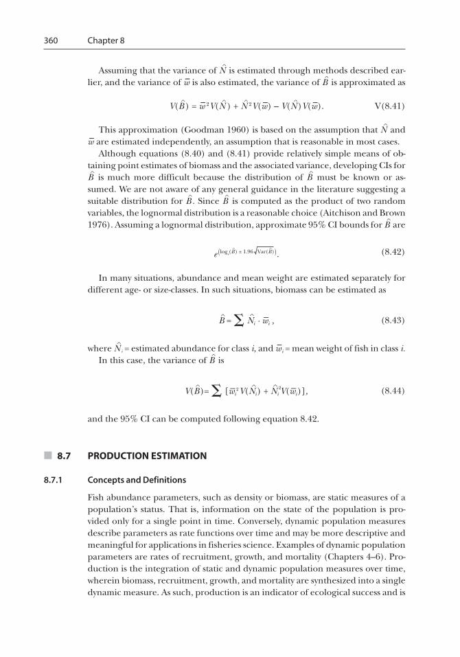
Assuming that the variance of N^ is estimated through methods described ear-
lier, and the variance of w– is also estimated, the variance of B^ is approximated as
V(B^) = w– 2V(N
^) + N
^2V(w–) – V(N^)V(w–). V(8.41)
This approximation (Goodman 1960) is based on the assumption that N^ and
w– are estimated independently, an assumption that is reasonable in most cases.Although equations (8.40) and (8.41) provide relatively simple means of ob-
taining point estimates of biomass and the associated variance, developing CIs forB^ is much more difficult because the distribution of B
^ must be known or as-
sumed. We are not aware of any general guidance in the literature suggesting asuitable distribution for B
^. Since B
^ is computed as the product of two random
variables, the lognormal distribution is a reasonable choice (Aitchison and Brown1976). Assuming a lognormal distribution, approximate 95% CI bounds for B
^ are
e (loge(B) ± 1.96 Var(B)).^ ^ (8.42)
In many situations, abundance and mean weight are estimated separately fordifferent age- or size-classes. In such situations, biomass can be estimated as
B = � Ni · wi ,^ ^ – (8.43)
where N^
i = estimated abundance for class i, and w–i = mean weight of fish in class i.In this case, the variance of B
^ is
V(B)= � [wi V(Ni) + Ni V(wi)],^ ^– 2
^ 2 – (8.44)
and the 95% CI can be computed following equation 8.42.
■ 8.7 PRODUCTION ESTIMATION
8.7.1 Concepts and Definitions
Fish abundance parameters, such as density or biomass, are static measures of apopulation’s status. That is, information on the state of the population is pro-vided only for a single point in time. Conversely, dynamic population measuresdescribe parameters as rate functions over time and may be more descriptive andmeaningful for applications in fisheries science. Examples of dynamic populationparameters are rates of recruitment, growth, and mortality (Chapters 4–6). Pro-duction is the integration of static and dynamic population measures over time,wherein biomass, recruitment, growth, and mortality are synthesized into a singledynamic measure. As such, production is an indicator of ecological success and is
Abundance, Biomass, and Production 361
especially responsive to environmental change (Mann and Penczak 1986). Thus,production rate of a fish population can be a useful measure and comparativetool, with many valuable applications for fisheries research and management.
Production is defined as the rate of tissue elaboration over time, regardless ofwhether it survives to the end of a given period (Waters 1977). It is expressed inunits of quantity/space/time, usually kilograms/hectare/year for fish populations.Production rate represents the flow of energy through trophic levels and may alsobe expressed in units of calories/hectare/year.
The methods and terminology for estimating fish production have evolved to agenerally accepted convention, and fish production estimates are routinely foundin the literature, especially for fishes of small streams and salmonid species. How-ever, many fisheries scientists rarely consider using this assessment tool, even thoughthey may regularly gather the data required to estimate production. Presumably,this occurs because the computations can be complex and cumbersome and aremore so if precision of production estimates and related parameters is estimated.The development of computer software and availability of other technical resourcesto minimize computation effort and reduce calculation error associated with theprocess of estimating production may increase the utility of this tool in fisheriesscience (Railsback et al. 1989; Kwak 1992).
8.7.2 Production Estimation Methods
Five methods to estimate production rate of aquatic animal populations have beendeveloped, refined, and accepted by ecologists (Waters 1977; Bagenal 1978;Chapman 1978). Some of these methods were originally intended for estimatingaquatic macroinvertebrate production but were readily adapted for use with fishpopulations. The five methods include two iterative summation methods, (1) theremoval summation and (2) increment summation methods; (3) the instanta-neous growth rate method and a graphical representation, (4) the Allen curve;and (5) the size-frequency method. Three of the methods (increment summa-tion, instantaneous growth rate, and size-frequency) have been refined for appli-cation to fish populations, and variance estimators for all parameters associatedwith those methods have been derived. All methods except the size-frequencymethod are cohort based, meaning that information on the age structure of thefish population is required.
Sampling requirements to estimate fish production are a series of absolute den-sity and biomass estimates (sections 8.3, 8.4, and 8.6) for a population within a 1-year period, with the first and last sampling dates occurring approximately 1 yearapart to estimate annual production. Cohort-based methods require stratificationand separate estimates by cohort; thus, data must be collected on population agestructure. In general, production is estimated by individual cohorts for a single timeinterval; then, those partial estimates are summed for all cohorts to yield a produc-tion estimate for the entire population during the specific interval. The productionestimate for a 1-year period (annual production) is the sum of the production esti-mates for intervals within the annual period. When the size-frequency method is
362 Chapter 8
used, individual losses from one size-group to the next are summed from meanvalues over the annual period to yield a production estimate.
8.7.2.1 Summation Methods
Summation methods to estimate production stem from the concept that tissuelost from, or accumulated by, a population over a series of time increments isequivalent to an estimate of production. The removal summation method involvesestimating the number of individuals lost, by mortality or other removal, from acohort over a time interval and coupling those data with biomass information,which results in an estimate of production for that cohort during that interval.These are then summed over intervals and cohorts to estimate annual produc-tion. Removal summation is not typically applied to fish populations, and algo-rithms to estimate associated variance are not readily available. As such, we rec-ommend the use of the more commonly used increment summation method inpreference to the removal summation method.
Similar to the removal summation method, but quantifying accumulation ratherthan loss, the increment summation method sums the growth increments of acohort over time. The growth increment is quantified as the increase in meanindividual weight over a time interval for each cohort, and this increment is mul-tiplied by the density of the cohort to obtain a production estimate for the cohortduring that interval. Production for each cohort is summed for the population,and production for each interval is summed for an annual estimate.
Explicit formulae for increment summation production estimation and associ-ated variance estimators for fish populations were developed by Newman andMartin (1983) as
P^ = N
–w– , (8.45)
where P = production for a given cohort within a specified interval; N–
= estimatedarithmetic mean cohort density from time t to t + 1; and w– = estimated change inmean weight of individuals in the cohort from time t to t + 1 (i.e., w– t + 1 – w– t).
Sampling variance of the production estimate can be estimated as (Goodman1960)
V(P^) = N
– 2V(w–) + (w–)2V(N–
) – V(N–
)V(w–), (8.46)
where V(w–) and V(N–
) are the estimated variances of w– and N–
, respectively.Algorithms to estimate variance of w– and N
– are found in Newman and Mar-
tin (1983) and require estimates of variance for each density and mean weightestimate (sections 8.3 and 8.6). The statistical software Pop/Pro (Kwak 1992; avail-able on CDROM) includes a module to estimate fish production by the incre-ment summation method according to cohort and time interval, including re-lated parameters and associated variances.
Abundance, Biomass, and Production 363
8.7.2.2 Instantaneous Growth Rate and Allen Curve Methods
The instantaneous growth rate method was initially developed to estimate pro-duction of fish populations (Ricker 1946; Allen 1949). By this method, produc-tion is estimated as simply the product of the estimated instantaneous growth rateand estimated mean biomass as
P^ = G
^B–
, (8.47)
where P^ = estimated production for a given cohort within a specified interval,
G^ = estimated instantaneous growth rate for the cohort from time t to t + 1 (i.e.,
loge w–
t + 1 – loge w–
t), and B–
= estimated arithmetic mean cohort biomass from timet to t + 1 (i.e., B
^
t + B^
t + 1)/2).From Newman and Martin (1983), the variance of the production estimate
may be estimated as
V(P^) = V(B
–)G
^2 + V(G^)B
–2, (8.48)
where V(B–
) and V(G^) are variances of the mean biomass and instantaneous growth
rate, respectively. The variance of mean biomass is estimated as
V(B–
) = [V(B^
t) + V(B^
t + 1)]/4 , (8.49)
where V(B^
t) and V(B^
t + 1) are the variances of biomass at times t and t + 1, respectively.The variance of the instantaneous growth rate may be estimated as
V(G^) = V(loge w
–t) + V(loge w
–t + 1), (8.50)
where V(loge w–
t) and V(loge w–
t + 1) are variances of the natural logarithms of esti-mated mean weights of individuals of the cohort at times t and t + 1, respectively.By using a Taylor series expansion (delta method; Seber 1982; Cone and Krueger1988), V(loge w
–t) can be approximated as
V(loge w–
t) = V(w– t)/w– t2. (8.51)
Mean annual density or biomass estimates (and their variances) computedfrom multiple intervals of different duration must be weighted according to thenumber of days in each interval (i.e., equations [8.47] and [8.48] must be modi-fied) and should be computed following formulae in Newman and Martin (1983).Fish production, including related parameters and associated variances, can beestimated according to cohort and time interval by the instantaneous growthrate method by means of Pop/Pro statistical software (Kwak 1992). Additionalalgorithms are available in the software documentation. An example calcula-tion of fish annual production estimated by the instantaneous growth rate methodis presented in Box 8.8.

364 Chapter 8
Box 8.8 Production Estimation Based on the Instantaneous Growth Rate Method
Density, mean weight, and biomass (and associated variances) of a brook trout population in ValleyCreek, Minnesota, were estimated in a stream reach with an area of 0.181 ha on four dates betweenMarch 1974 and March 1975 (Waters 1999). Population statistics for two of these dates are pre-sented below in order to illustrate how to estimate production using the instantaneous growth ratemethod.
Table Population statistics for brook trout in Valley Creek, Minnesota.
Age-class Density Mean weight Biomassand total (N
^
) V(N^
) (w–, g) V(w– ) (B^
, g) V(B^)
Sampling date: 8 March 19741 277.85 1,336.05 6.86 0.13 1,905.34 75,455.972 157.54 317.71 28.56 0.79 4,499.83 222,126.453 36.11 34.00 107.23 19.89 3,872.13 469,764.754 11.17 13.16 170.05 42.09 1,898.89 350,364.34
Total 482.67 1,700.92 12,176.19 1,117,711.51
Sampling date: 29 July 19741 276.45 553.56 24.27 0.62 6,709.17 306,074.532 68.08 94.58 77.31 2.49 5,262.90 278,582.663 9.76 7.64 146.18 100.67 1,427.00 167,558.974 8.12 1.11 194.72 1.67 1,582.12 30,259.81
Total 362.41 656.89 14,981.19 782,475.97
To estimate production for the age-1 cohort during this interval, we follow equation (8.47) as
P^
= GB–, or
P^
= (loge24.27 – loge6.86)[(6,709.17 + 1,905.34)/2] = 5,442.36g.
where P^
is the estimated production and G is the estimated instantaneous growth rate for a givencohort within a specified interval. To estimate the variance of P
^, we begin by estimating the
variance B–
of from equation (8.49) as
V(B–
) = [V(Bt) + V(Bt + 1)]/4, orV(B
–) = (75,455.97 + 306,074.53/4 = 95,383.62g.
Allen (1951) extended the instantaneous growth rate method to a graphicalform to estimate production in what has become known as the Allen curve method.The Allen curve is a growth–survivorship curve for a given cohort, wherein thenumber of surviving individuals is plotted against the mean weight of those indi-viduals (Figure 8.6). Following this configuration, the biomass of the cohort canbe estimated at any point in time on the curve as the corresponding product ofnumber of individuals (or density) and their mean weight. Likewise, the area
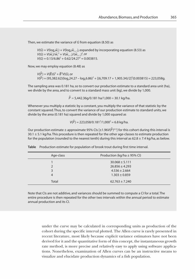
Abundance, Biomass, and Production 365
Then, we estimate the variance of G from equation (8.50) as
V(G) = V(logew–t) + V(logew–t + 1), expanded by incorporating equation (8.53) asV(G) = V(w–t)/w–t
2 + V(w–t + 1)/(w–t + 1)2, orV(G) = 0.13/6.862 + 0.62/24.272 = 0.003815.
Now, we may employ equation (8.48) as
V(P^
) = V(B–
)G2 + B–2V(G), or
V(P^
) = (95,382.62)(loge24.27 – loge6.86)2 + [(6,709.17 + 1,905.34)/2]2(0.003815) = 223,058g.
The sampling area was 0.181 ha, so to convert our production estimate to a standard area unit (ha),we divide by the area, and to convert to a standard mass unit (kg), we divide by 1,000.
P^
= 5,442.36g/0.181 ha/1,000 = 30.1 kg/ha.
Whenever you multiply a statistic by a constant, you multiply the variance of that statistic by theconstant squared. Thus, to convert the variance of our production estimate to standard units, wedivide by the area (0.181 ha) squared and divide by 1,000 squared as
V(P^
) = 223,058/0.1812/1,0002 = 6.8 kg/ha.
Our production estimate ± approximate 95% CIs [±1.96V(P^
)0.5] for this cohort during this interval is30.1 ± 5.1 kg/ha. This procedure is then repeated for the other age-classes to estimate productionfor the population (rounded to the nearest tenth) during this interval as 62.8 ± 7.4 kg/ha, as below.
Table Production estimate for population of brook trout during first time interval.
Age-class Production (kg/ha ± 95% CI)
1 30.068 ± 5.1112 26.856 ± 4.2933 4.536 ± 2.6644 1.303 ± 0.859
Total 62.763 ± 7.240
Note that CIs are not additive, and variances should be summed to compute a CI for a total. Theentire procedure is then repeated for the other two intervals within the annual period to estimateannual production and its CI.
under the curve may be calculated in corresponding units as production of thecohort during the specific interval plotted. The Allen curve is rarely presented inrecent literature, most likely because explicit variance estimators have not beenderived for it and the quantitative form of this concept, the instantaneous growthrate method, is more precise and relatively easy to apply using software applica-tions. Nonetheless, examination of Allen curves can be an instructive means tovisualize and elucidate production dynamics of a fish population.
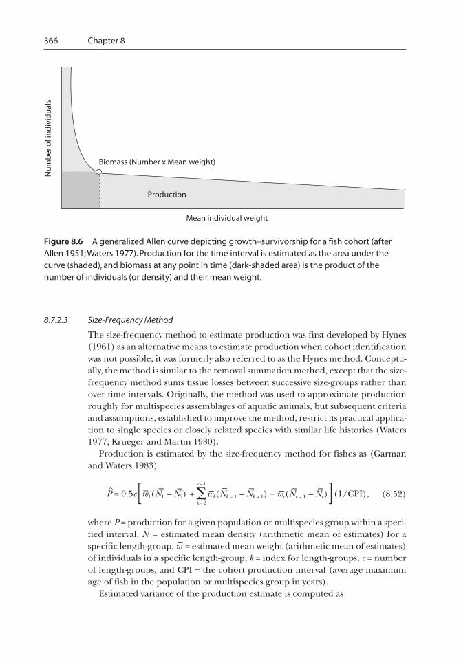
366 Chapter 8
8.7.2.3 Size-Frequency Method
The size-frequency method to estimate production was first developed by Hynes(1961) as an alternative means to estimate production when cohort identificationwas not possible; it was formerly also referred to as the Hynes method. Conceptu-ally, the method is similar to the removal summation method, except that the size-frequency method sums tissue losses between successive size-groups rather thanover time intervals. Originally, the method was used to approximate productionroughly for multispecies assemblages of aquatic animals, but subsequent criteriaand assumptions, established to improve the method, restrict its practical applica-tion to single species or closely related species with similar life histories (Waters1977; Krueger and Martin 1980).
Production is estimated by the size-frequency method for fishes as (Garmanand Waters 1983)
(8.52)
where P = production for a given population or multispecies group within a speci-fied interval, N
– = estimated mean density (arithmetic mean of estimates) for a
specific length-group, w– = estimated mean weight (arithmetic mean of estimates)of individuals in a specific length-group, k = index for length-groups, c = numberof length-groups, and CPI = the cohort production interval (average maximumage of fish in the population or multispecies group in years).
Estimated variance of the production estimate is computed as
Figure 8.6 A generalized Allen curve depicting growth–survivorship for a fish cohort (afterAllen 1951; Waters 1977). Production for the time interval is estimated as the area under thecurve (shaded), and biomass at any point in time (dark-shaded area) is the product of thenumber of individuals (or density) and their mean weight.
Nu
mb
er o
f in
div
idu
als
Mean individual weight
Production
Biomass (Number x Mean weight)
P = 0.5c[w1(N1 – N2) + �wk(Nk – 1 – Nk + 1) + wc(Nc – 1 – Nc)](1/CPI),^ –
·
– –k = 2
c – 1
– – – – – –

Abundance, Biomass, and Production 367
(8.53)
where V(N–
) and V(w–) are variances of mean density and mean weight, respec-tively, for length-groups. If the production period spans more than a single timeinterval (more than two samples), then mean density and mean weight estimates(and associated variances) must be weighted by interval length (days) accordingto algorithms provided by Garman and Waters (1983). An example calculation offish annual production estimated by the size-frequency method is presented inBox 8.9.
8.7.3 Production to Mean Biomass (P/B–
) Ratio
The annual production to annual mean biomass (P/B–
) ratio is of special interestas an ecological index (also referred to as the turnover ratio) and as a simpleconversion factor to approximate production (Waters 1977). Based on the premisethat P/B
– is relatively constant for an organism or related organisms, it has been
suggested that production may be approximated from a biomass estimate usingthe P/B
– ratio as a multiplier. The ratio of P/B
– for most fish species varies from 0.2
to 4.0. However, P/B–
can be quite variable within and among species (Waters1977, 1999; Mann and Penczak 1986; Elliott 1994) and may vary with the numberof cohorts (or life span) of a population (Waters 1992; Kwak and Waters 1997).Thus, this method should be applied carefully and considered an imprecise ap-proximation of production. The exact P/B
– ratio to employ for such estimates
should be species specific and may be refined further if the number of cohorts in apopulation is known (Waters 1992; Kwak and Waters 1997). Estimates of mean an-nual biomass should be weighted by interval duration if more than a single intervalis included. Newman and Martin (1983) present formulae for estimating meanannual biomass and its variance, as well as a variance estimator for the P/B
– ratio.
8.7.4 Production Estimates in Practice
In general, if age data are available, the instantaneous growth rate method is thepreferred approach to estimate fish production and associated parameters; other-wise, the size-frequency method may be used. Estimating production using the P/B
–
ratio should be used only when data are lacking for application of more precisemethods. Computer software is available for using the increment summation orinstantaneous growth rate methods (Kwak 1992; available at http://www4.ncsu.edu/~tkwak), and a spreadsheet application can facilitate calculations by othermethods. Estimates of variance (precision or sampling error) should be reportedfor all estimates of production and related population parameters as approximate95% CIs.
V(P) = (0.5c)2^ –
– –
k = 2
c – 1 ––
– – – –
{ (w1 + w2)2V(N1) + V(w1)(N1 – N2)
2
�[(wk – 1 – wk + 1)2V(Nk) + V(wk)(Nk – 1 – Nk + 1)
2]– – –+
+ (wc – 1 – wc)2V(Nc ) + V(wc )(Nc – 1 – Nc )
2– – – – – – } (1/CPI)2 ,
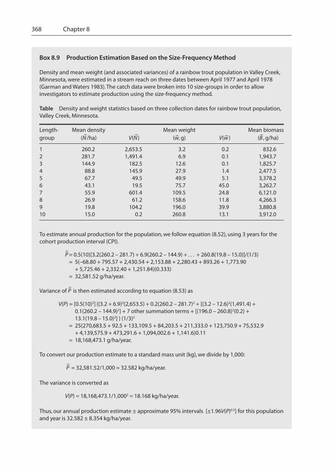
368 Chapter 8
Box 8.9 Production Estimation Based on the Size-Frequency Method
Density and mean weight (and associated variances) of a rainbow trout population in Valley Creek,Minnesota, were estimated in a stream reach on three dates between April 1977 and April 1978(Garman and Waters 1983). The catch data were broken into 10 size-groups in order to allowinvestigators to estimate production using the size-frequency method.
Table Density and weight statistics based on three collection dates for rainbow trout population,Valley Creek, Minnesota.
Length- Mean density Mean weight Mean biomassgroup (N
–/ha) V(N
–) (w–, g) V(w– ) (B
–, g/ha)
1 260.2 2,653.5 3.2 0.2 832.62 281.7 1,491.4 6.9 0.1 1,943.73 144.9 182.5 12.6 0.1 1,825.74 88.8 145.9 27.9 1.4 2,477.55 67.7 49.5 49.9 5.1 3,378.26 43.1 19.5 75.7 45.0 3,262.77 55.9 601.4 109.5 24.8 6,121.08 26.9 61.2 158.6 11.8 4,266.39 19.8 104.2 196.0 39.9 3,880.810 15.0 0.2 260.8 13.1 3,912.0
To estimate annual production for the population, we follow equation (8.52), using 3 years for thecohort production interval (CPI).
P^
= 0.5(10)[3.2(260.2 – 281.7) + 6.9(260.2 – 144.9) + . . . + 260.8(19.8 – 15.0)]/(1/3)= 5(–68.80 + 795.57 + 2,430.54 + 2,153.88 + 2,280.43 + 893.26 + 1,773.90
+ 5,725.46 + 2,332.40 + 1,251.84)(0.333)= 32,581.52 g/ha/year.
Variance of P^
is then estimated according to equation (8.53) as
V(P) = [0.5(10)2] {(3.2 + 6.9)2(2,653.5) + 0.2(260.2 – 281.7)2 + [(3.2 – 12.6)2(1,491.4) +0.1(260.2 – 144.9)2] + 7 other summation terms + [(196.0 – 260.8)2(0.2) +13.1(19.8 – 15.0)2] } (1/3)2
= 25(270,683.5 + 92.5 + 133,109.5 + 84,203.5 + 211,333.0 + 123,750.9 + 75,532.9+ 4,139,575.9 + 473,291.6 + 1,094,002.6 + 1,141.6)0.11
= 18,168,473.1 g/ha/year.
To convert our production estimate to a standard mass unit (kg), we divide by 1,000:
P^
= 32,581.52/1,000 = 32.582 kg/ha/year.
The variance is converted as
V(P) = 18,168,473.1/1,0002 = 18.168 kg/ha/year.
Thus, our annual production estimate ± approximate 95% intervals [±1.96V(P)0.5] for this populationand year is 32.582 ± 8.354 kg/ha/year.

Abundance, Biomass, and Production 369
Many assumptions and criteria for applying these methods have been definedand should be considered with application (Waters 1977; Newman and Martin1983). We suggest that subjective decisions encountered when estimating fishproduction should be resolved to be conservative, so that the direction of errorwill be clear, and estimates may be considered minimums. The biomass estimateof age-0 fish, newly recruited into the population, at first sampling should beconsidered a conservative estimate of production for that cohort during that in-terval. Negative estimates of production, resulting from negative growth (i.e.,weight loss), should be interpreted as no production (zero) for that cohort andinterval when using summation methods or the instantaneous growth rate method.However, negative losses (i.e., increase in numbers between size-groups) shouldbe included in the sum when applying the size-frequency method.
Generally, the greater the number of fish population estimates (density andbiomass) that are integrated into an annual production estimate, the more accu-rate that estimate will be. The minimum number of two population estimates willyield a less accurate production estimate than will one based on more estimateswithin the annual period. A reasonable, general approach to estimating popula-tions over a 1-year period for an annual production estimate is to conduct oneestimate prior to spawning (e.g., spring for many temperate fishes), another nearthe end of the primary growing season (e.g., fall for temperate areas), and a third1 year after the first estimate (e.g., spring or fall).
Fish production estimates are valuable statistics for understanding populationdynamics and elucidating ecological relationships and have great potential forimproving fisheries management. Waters (1992) reviewed and proposed the ap-plication of annual production, annual P/B
– ratio, and ecotrophic coefficient (an-
nual angler harvest/annual production) to management of stream-dwelling troutfisheries. Incorporating production dynamics into fish assessment and monitor-ing may provide a broader perspective on the dynamics of harvested fishes. Thus,regulation and assessment of harvest as a proportion of fish tissue produced onan annual basis provides an alternative to the standard approach, based solely onfish density or biomass.
■ 8.8 FUTURE DIRECTIONS
In many studies of fish populations, information is often available beyond thatneeded to apply the methods outlined in this chapter. In particular, informationon the age structure of the population is often collected. When the abundance ofa population is estimated on an annual basis, knowledge of the prior age compo-sition is helpful in constraining estimates. As a simple example, the abundance ofa cohort cannot be larger than the abundance in the prior year (in a closed popu-lation). The constraints imposed by age structure relationships can help improvethe precision and accuracy of population estimates. Application of auxiliary infor-mation to population estimation opens up a diversity of models. Powerful statisti-cal catch-at-age models (Hilborn and Walters 1992) are an example of a frame-work that incorporates the extensive information that is often available on
370 Chapter 8
intensively studied fish populations. Because of the complexity of such modelsand their intensive data needs, such methods are generally applied to marine fishstocks and some stocks in large inland waters (e.g., Great Lakes) where the cost ofdata collection and analysis is commensurate with the value of the fishery.
Even within the scope of the methods presented in this chapter, there are po-tential gains to be made by combining data from different sources. In particular,the combination of removal methods with marking fish holds promise for improv-ing population estimates. The methods illustrated here for analyzing mark–re-capture data do not make direct use of measures of sampling effort. Removalmethods, on the other hand, explicitly assume effort is constant or accommodatechanges in effort by standardizing catch to C/f.
The estimation of the variance and CIs for population estimates is an areawhere substantial improvements need to be made. Although the likelihood meth-ods presented here have a long history of use, and provide a strong statistical basisfor estimation, many of the formulae are strictly valid only for large sample sizesor are approximations to the “full” formulae. In many applications, the targetpopulation itself may be small (e.g., the number of fish in a 100-m stretch ofstream) or the number of marked or recaptured fish is small to moderate (i.e.,less than 30). In situations like these, variance estimates and CIs should be inter-preted with caution.
A trend we see emerging is the incorporation of a Bayesian approach to dataanalysis. In many situations, researchers and managers have knowledge from priorexperience that is pertinent to the population being studied. Incorporating theexperience and beliefs of experts can improve population estimates in many cases(Hilborn and Walters 1992). The Bayesian approach, however, presents severalpractical concerns regarding how best to represent prior information.
■ 8.9 CONCLUSIONS
In this chapter, we illustrate several approaches for estimating fish abundance,biomass, and production. A foundational concept is that additional informationbeyond C/f is generally needed to provide accurate population estimates. Theincorporation of this information inevitably entails making assumptions aboutthe sampling regime and creating models of this idealized process. Therefore, itis important to test assumptions, where possible, and apply models that best rep-resent the data obtained. Some assumptions can be relaxed by applying alternatemodels, but some are essential to obtain any valid estimate. The key to meetingcritical assumptions is often the judicious planning of the sampling program andthe careful application of field methods. Given the wide array of sampling chal-lenges facing fisheries scientists, this chapter should be viewed as an entry intosome of the more common and basic methods. Every investigation poses its ownset of challenges, but often these problems are not unique. By building on thebase developed here, we hope to provide readers with the confidence to face thediversity of situations they are likely to encounter in their professional work.

Abundance, Biomass, and Production 371
■ 8.10 REFERENCES
Aitchison, J., and J. A. C. Brown. 1976. The lognormal distribution with special referenceto its uses in economics. Cambridge University Press, Cambridge, UK.
Akaike, H. 1973. Information theory and an extension of the maximum likelihood princi-pal. Pages 267–281 in B. N. Petran and F. Csaki, editors. International symposium oninformation theory, 2nd edition. Akademiai Kiadi, Budapest.
Allen, K. R. 1949. Some aspects of the production and cropping of fresh waters. Transac-tions of the Royal Society of New Zealand 77(5):222–228.
Allen, K. R. 1951. The Horokiwi Stream. New Zealand Marine Department Fishery Bul-letin 10.
Anderson, R. O., and R. M. Neumann. 1996. Length, weight, and associated structuralindices. Pages 447–482 in B. R. Murphy and D. W. Willis, editors. Fisheries techniques,2nd edition. American Fisheries Society, Bethesda, Maryland.
Bagenal, T. 1978. Methods for assessment of fish production in fresh waters. IBP (Interna-tional Biological Programme) Handbook No. 3, Blackwell Scientific Publications, Ox-ford, UK.
Bickel, P. J., and K. A. Doksum. 1977. Mathematical statistics: basic ideas and selectedtopics. Holden-Day, San Francisco.
Buckland, S. T., D. R. Anderson, K. P. Burnham, and J. L. Laake. 1993. Distance sampling:estimating abundance of biological populations. Chapman and Hall, London.
Burnham, K. P., D. R. Anderson, G. C. White, C. Brownie, and K. H. Pollock. 1987. Designand analysis methods for fish survival experiments based on release–recapture. Ameri-can Fisheries Society, Monograph 5, Bethesda, Maryland.
Chapman, D. G. 1948. A mathematical study of confidence limits of salmon populationscalculated from sample tag ratios. International Pacific Salmon Fisheries CommissionBulletin 2:69–85.
Chapman, D. G. 1951. Some properties of the hypergeometric distribution with applica-tions to zoological censuses. University of California Publications in Statistics 1:131–160.
Chapman, D. W. 1978. Production in fish populations. Pages 5–25 in S. D. Gerking, editor.Ecology of freshwater fish production. Blackwell Scientific Publications, Oxford, UK.
Collie, J. S., and M. P. Sissenwine. 1983. Estimating population size from relative abun-dance data measured with error. Canadian Journal of Fisheries and Aquatic Sciences40:1871–1879.
Cone, R. S., and C. C. Krueger. 1988. Comparison of survival, emigration, habitat use,marking mortality, and growth between two strains of brook trout in Adirondack ponds.North American Journal of Fisheries Management 8:497–504.
De Lury, D. B. 1947. On the estimation of biological populations. Biometrics 3:145–167.Edwards, E. F., and B. A. Megrey. 1989. Mathematical analysis of fish stock dynamics. Ameri-
can Fisheries Society, Symposium 6, Bethesda, Maryland.Elliott, J. M. 1994. Quantitative ecology and the brown trout. Oxford University Press,
Oxford, UK.Foote, K. G., and G. Stefansson. 1993. Definition of the problem of estimating fish abun-
dance over an area from acoustic line-transect measurements of density. ICES Journalof Marine Science 50:369–381.
372 Chapter 8
Garman, G. C., and T. F. Waters. 1983. Use of the size-frequency (Hynes) method to esti-mate annual production of a stream fish population. Canadian Journal of Fisheries andAquatic Sciences 40:2030–2034.
Goodman, L. A. 1960. On the exact variance of products. Journal of the American Statis-tical Association 55:708–713.
Gould, W. R., and K. H. Pollock. 1997. Catch-effort maximum likelihood estimation ofimportant population parameters. Canadian Journal of Fisheries and Aquatic Sciences54:890–897.
Hankin, D. G., and G. H. Reeves. 1988. Estimating total fish abundance and total habitatarea in small streams based on visual estimation methods. Canadian Journal of Fisher-ies and Aquatic Sciences 45:834–844.
Heimbuch, D. G., H. T. Wilson, S. B. Weisberg, and J. H. Volstad. 1997. Estimating fishabundance in stream surveys by using double-pass removal sampling. Transactions ofthe American Fisheries Society 126:795–803.
Hilborn, R., and C. J. Walters. 1992. Quantitative fisheries stock assessment: choice, dy-namics and uncertainty. Chapman and Hall, New York.
Hynes, H. B. N. 1961. The invertebrate fauna of a Welsh mountain stream. Archiv furHydrobiologia 57:344–388.
Junge, C. O., and J. Libosvárský. 1965. Effects of size selectivity on population estimatesbased on successive removals with electrical fishing gear. Zoological Listy 14:171–178.
Krueger, C. C., and F. B. Martin. 1980. Computation of confidence intervals for the size-frequency (Hynes) method of estimating secondary production. Limnology and Ocean-ography 25:773–777.
Kwak, T. J. 1992. Modular microcomputer software to estimate fish population param-eters, production rates and associated variance. Ecology of Freshwater Fish 1:73–75.(Software available at http://www4.ncsu.edu/~tkwak.)
Kwak, T. J., and T. F. Waters. 1997. Trout production dynamics and water quality in Minne-sota streams. Transactions of the American Fisheries Society 126:35–48.
Lebreton, J-D., K. P. Burnham, J. Clobert, and D. R. Anderson. 1992. Modeling survivaland testing biological hypotheses using marked animals: a unified approach with casestudies. Ecological Monographs 62:67–118.
Leslie, P. H., and D. H. S. Davis. 1939. An attempt to determine the absolute number ofrats on a given area. Journal of Animal Ecology 8:94–113.
Ludwig, D., and C. J. Walters. 1985. Are age-structured models appropriate for catch-effort data? Canadian Journal of Fisheries and Aquatic Sciences 42:1066–1072.
Mann, R. H. K., and T. Penczak. 1986. Fish production in rivers: a review. Polskie ArchiwumHydrobiologii 33:233–247.
Mesnil, B. 2003. The catch-survey analysis (CSA) method of fish stock assessment: an evalu-ation using simulated data. Fisheries Research 63:193–212.
Newman, R. M., and F. B. Martin. 1983. Estimation of fish production rates and associatedvariances. Canadian Journal of Fisheries and Aquatic Sciences 40:1729–1736.
Otis, D. L., K. P. Burnham, G. C. White, and D. R. Anderson. 1978. Statistical inference forcapture data from closed populations. Wildlife Monographs 62.
Railsback, S. F., B. D. Holcomb, and M. G. Ryon. 1989. A computer program for estimat-ing fish population sizes and annual production rates. Oak Ridge National Laboratory,Environmental Sciences Division Publication 3245, Oak Ridge, Tennessee.
Abundance, Biomass, and Production 373
Rice, J. A. 1995. Mathematical statistics and data analysis, 2nd edition. Duxbury Press,Belmont, California.
Ricker, W. E. 1946. Production and utilization of fish populations. Ecological Monographs16:373–391.
Ricker, W. E. 1977. Computation and interpretation of biological statistics of fish popula-tions. Department of the Environment, Fisheries and Marine Service, Bulletin 191,Ottawa.
Robson, D. S., and H. A. Regier. 1964. Sample size in Petersen mark–recapture experi-ments. Transactions of the American Fisheries Society 93:215–226.
Schnabel, Z. E. 1938. The estimation of the total fish population of a lake. AmericanMathematical Monographs 45:348–352.
Schnute, J. 1983. A new approach to estimating populations by the removal method. Ca-nadian Journal of Fisheries and Aquatic Sciences 40:2153–2169.
Schnute, J. T., L. J. Richards, and N. Olsen. 1998. Statistics, software, and fish stock assess-ment. Pages 171–184 in F. Funk and seven coeditors. Fishery stock assessment models.University of Alaska, Sea Grant College Program AK-SG-98–01, Anchorage.
Seber, G. A. F. 1982. The estimation of animal abundance and related parameters. EdwardArnold, London.
Seber, G. A. F., and C. J. Wild. 1989. Nonlinear regression. Wiley, New York.Thomas, L., and nine coauthors. 2001. Distance 4.0. Beta 2. Research Unit for Wildlife
Population Assessment, University of St. Andrews, UK.Thompson, W. L., G. C. White, and C. Gowan. 1998. Monitoring vertebrate populations.
Academic Press, San Diego, California.Van Deventer, J. S., and W. S. Platts. 1989. Microcomputer software system for generating
population statistics from electrofishing data—user’s guide for MicroFish 3.0. U.S. For-est Service, Intermountain Research Station, General Technical Report INT-254, Ogden,Utah.
Vondracek, B., and D. J. Degan. 1995. Among- and within-transect variability in estimatesof shad abundance made with hydroacoustics. North American Journal of FisheriesManagement 15:933–939.
Waters, T. F. 1977. Secondary production in inland waters. Advances in Ecological Re-search 10:91–164.
Waters, T. F. 1992. Annual production, production/biomass ratio, and the ecotrophiccoefficient for management of trout in streams. North American Journal of FisheriesManagement 12:34–39.
Waters, T. F. 1999. Long-term trout production dynamics in Valley Creek, Minnesota. Trans-actions of the American Fisheries Society 128:1151–1162.
White, G. C., and K. P. Burnham. 1999. Program MARK: survival estimation from popula-tions of marked animals. Bird Study 46 (Supplement):120–138.
Zippin, C. 1956. An evaluation of the removal method of estimating animal population.Biometrics 12:163–169.
Zippin, C. 1958. The removal method of population estimation. Journal of Wildlife Man-agement 22:82–90.

374 Chapter 8
Appendix Shortest 95% confidence interval (CI) for the population estimate N(Reproduced from Chapman 1948).
Confidence intervals for sample sizes of 50 or less are based on the Poisson distribution. The number ofrecaptures is denoted by m, and estimates of the CI for N are obtained by multiplying the table values bythe product of the number of fish caught in the first and second sample (i.e., n1 · n2).
CI CI
m Lower limit Upper limit m Lower limit Upper limit
0 0.0885 26 0.02478 0.05631 0.0720 19.489 27 0.02408 0.05392 0.0767 2.821 28 0.02342 0.05163 0.0736 1.230 29 0.02279 0.04954 0.0690 0.738 30 0.02221 0.04755 0.0644 0.513 31 0.02165 0.04576 0.0600 0.388 32 0.02112 0.04407 0.0561 0.309 33 0.02061 0.04258 0.0526 0.256 34 0.02014 0.04109 0.0495 0.217 35 0.01968 0.039610 0.0468 0.188 36 0.01925 0.038411 0.0443 0.165 37 0.01883 0.037212 0.0420 0.147 38 0.01843 0.036013 0.0400 0.133 39 0.01805 0.035014 0.0382 0.121 40 0.01769 0.0339615 0.0365 0.111 41 0.01733 0.0330016 0.0350 0.1020 42 0.01700 0.0321017 0.03362 0.0945 43 0.01668 0.0312418 0.03233 0.0880 44 0.01636 0.0304319 0.03114 0.0823 45 0.01606 0.0296620 0.03004 0.0773 46 0.01578 0.0289221 0.02901 0.0729 47 0.01550 0.0282222 0.02806 0.0689 48 0.01523 0.0275523 0.02716 0.0653 49 0.01498 0.0269124 0.02632 0.0620 50 0.01475 0.0262525 0.02552 0.0591