7th International Workshop onUncertainty Reasoning for the

Semantic Web

Proceedings

edited by Fernando Bobillo

Rommel Carvalho

Paulo C. G. da Costa

Claudia d’Amato

Nicola Fanizzi

Kathryn B. Laskey

Kenneth J. Laskey

Thomas Lukasiewicz

Trevor Martin

Matthias Nickles

Michael Pool

Bonn, Germany, October 23, 2011

collocated with

the 10th International Semantic Web Conference

– ISWC 2011 –

II

Foreword

This volume contains the papers presented at the 7th International Work-shop on Uncertainty Reasoning for the Semantic Web (URSW 2011), held asa part of the 10th International Semantic Web Conference (ISWC 2011) atBonn, Germany, October 23, 2011. It contains 8 technical papers and 3 posi-tion papers, which were selected in a rigorous reviewing process, where eachpaper was reviewed by at least four program committee members.

The International Semantic Web Conference is a major international fo-rum for presenting visionary research on all aspects of the Semantic Web. TheInternational Workshop on Uncertainty Reasoning for the Semantic Web isan exciting opportunity for collaboration and cross-fertilization between theuncertainty reasoning community and the Semantic Web community. Effectivemethods for reasoning under uncertainty are vital for realizing many aspectsof the Semantic Web vision, but the ability of current-generation web tech-nology to handle uncertainty is extremely limited. Recently, there has been agroundswell of demand for uncertainty reasoning technology among SemanticWeb researchers and developers. This surge of interest creates a unique open-ing to bring together two communities with a clear commonality of interestbut little history of interaction. By capitalizing on this opportunity, URSWcould spark dramatic progress toward realizing the Semantic Web vision.

We wish to thank all authors who submitted papers and all workshopparticipants for fruitful discussions. We would like to thank the program com-mittee members and external referees for their timely expertise in carefullyreviewing the submissions.

October 2011Fernando Bobillo

Rommel CarvalhoPaulo C. G. da Costa

Claudia d’AmatoNicola Fanizzi

Kathryn B. LaskeyKenneth J. Laskey

Thomas LukasiewiczTrevor Martin

Matthias NicklesMichael Pool

III

IV

Workshop Organization

Program Chairs

Fernando Bobillo (University of Zaragoza, Spain)Rommel Carvalho (George Mason University, USA)Paulo C. G. da Costa (George Mason University, USA)Claudia d’Amato (University of Bari, Italy)Nicola Fanizzi (University of Bari, Italy)Kathryn B. Laskey (George Mason University, USA)Kenneth J. Laskey (MITRE Corporation, USA)Thomas Lukasiewicz (University of Oxford, UK)Trevor Martin (University of Bristol, UK)Matthias Nickles (University of Bath, UK)Michael Pool (Vertical Search Works, Inc., USA)

Program Committee

Fernando Bobillo (University of Zaragoza, Spain)Silvia Calegari (University of Milano-Bicocca, Italy)Rommel Carvalho (George Mason University, USA)Paulo C. G. da Costa (George Mason University, USA)Fabio Gagliardi Cozman (Universidade de Sao Paulo, Brazil)Claudia d’Amato (University of Bari, Italy)Nicola Fanizzi (University of Bari, Italy)Marcelo Ladeira (Universidade de Brasılia, Brazil)Kathryn B. Laskey (George Mason University, USA)Kenneth J. Laskey (MITRE Corporation, USA)Thomas Lukasiewicz (University of Oxford, UK)Trevor Martin (University of Bristol, UK)Matthias Nickles (University of Bath, UK)Jeff Z. Pan (University of Aberdeen, UK)Rafael Penaloza (TU Dresden, Germany)Michael Pool (Vertical Search Works, Inc., USA)Livia Predoiu (University of Mannheim, Germany)Guilin Qi (Southeast University, China)Celia Ghedini Ralha (Universidade de Brasılia, Brazil)

V

David Robertson (University of Edinburgh, UK)Daniel Sanchez (University of Granada, Spain)Thomas Scharrenbach (University of Zurich, Switzerland)Sergej Sizov (University of Koblenz-Landau, Germany)Giorgos Stoilos (University of Oxford, UK)Umberto Straccia (ISTI-CNR, Italy)Andreas Tolk (Old Dominion University, USA)Peter Vojtas (Charles University Prague, Czech Republic)

VI

Table of Contents

Technical Papers

– Building A Fuzzy Knowledge Body for Integrating Domain Ontologies 3-14Konstantin Todorov, Peter Geibel, Celine Hudelot

– Estimating Uncertainty of Categorical Web Data 15-26Davide Ceolin, Willem Robert Van Hage, Wan Fokkink, Guus Schreiber

– An Evidential Approach for Modeling and Reasoning on Uncertainty in Se-mantic Applications 27-38Amandine Bellenger, Sylvain Gatepaille, Habib Abdulrab, Jean-Philippe Ko-towicz

– Representing Sampling Distributions in P-SROIQ 39-50Pavel Klinov, Bijan Parsia

– Finite Lattices Do Not Make Reasoning in ALCI Harder 51-62Stefan Borgwardt, Rafael Penaloza

– Learning Terminological Naive Bayesian Classifiers under Different Assump-tions on Missing Knowledge 63-74Pasquale Minervini, Claudia d’Amato, Nicola Fanizzi

– A Distribution Semantics for Probabilistic Ontologies 75-86Elena Bellodi, Evelina Lamma, Fabrizio Riguzzi, Simone Albani

– Semantic Link Prediction through Probabilistic Description Logics 87-97Kate Revoredo, Jose Eduardo Ochoa Luna, Fabio Gagliardi Cozman

Position Papers

– Distributed Imprecise Design Knowledge on the Semantic Web 101-104Julian R. Eichhoff, Wolfgang Maass

– Reasoning under Uncertainty with Log-Linear Description Logics 105-108Mathias Niepert

– Handling Uncertainty in Information Extraction 109-112Maurice Van Keulen, Mena B. Habib

VII

VIII

Technical Papers

2

Building A Fuzzy Knowledge Body forIntegrating Domain Ontologies

Konstantin Todorov1, Peter Geibel2, and Celine Hudelot1

1Laboratory MAS, Ecole Centrale Paris2TU Berlin, Sekr. FR 5-8, Fakultat IV

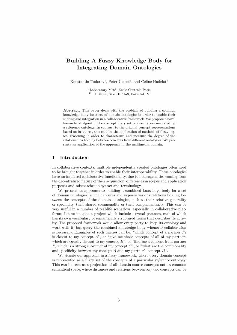
Abstract. This paper deals with the problem of building a commonknowledge body for a set of domain ontologies in order to enable theirsharing and integration in a collaborative framework. We propose a novelhierarchical algorithm for concept fuzzy set representation mediated bya reference ontology. In contrast to the original concept representationsbased on instances, this enables the application of methods of fuzzy log-ical reasoning in order to characterize and measure the degree of therelationships holding between concepts from different ontologies. We pre-senta an application of the approach in the multimedia domain.

1 Introduction

In collaborative contexts, multiple independently created ontologies often needto be brought together in order to enable their interoperability. These ontologieshave an impaired collaborative functionality, due to heterogeneities coming fromthe decentralized nature of their acquisition, differences in scopes and applicationpurposes and mismatches in syntax and terminology.

We present an approach to building a combined knowledge body for a setof domain ontologies, which captures and exposes various relations holding be-tween the concepts of the domain ontologies, such as their relative generalityor specificity, their shared commonality or their complementarity. This can bevery useful in a number of real-life scenarioss, especially in collaborative plat-forms. Let us imagine a project which includes several partners, each of whichhas its own vocabulary of semantically structured terms that describes its activ-ity. The proposed framework would allow every party to keep its ontology andwork with it, but query the combined knowledge body whenever collaborationis necessary. Examples of such queries can be: “which concept of a partner P1

is closest to my concept A”, or “give me those concepts of all of my partnerswhich are equally distant to my concept B”, or “find me a concept from partnerP2 which is a strong subsumer of my concept C”, or ”what are the commonalityand specificity between my concept A and my partner’s concept D“.

We situate our approach in a fuzzy framework, where every domain conceptis represented as a fuzzy set of the concepts of a particular reference ontology.This can be seen as a projection of all domain source concepts onto a commonsemantical space, where distances and relations between any two concepts can be

3

expressed under fixed criteria. In contrast to the original instance-representation,we can apply methods of fuzzy logical reasoning in order to characterize therelationship between concepts from different ontologies. In addition, the fuzzyrepresentations allow for quantifying the degree to which a certain relation holds.

The paper is structured as follows. Related work is presented in the nextsection. Background in the field of fuzzy sets, as well as main definitions andproblems from the ontology matching domain are overviewed in Section 3. Wepresent the concept fuzzification algorithm in Section 4, before we discuss howthe combined knowledge body can be constructed in Section 5. Experimentalresults and conclusions are presented in Sections 6 and 7, respectively.

2 Related Work

Fuzzy set theory generalizes classical set theory [19] allowing to deal with impre-cise and vague data. A way of handling imprecise information in ontologies is toincorporate fuzzy reasoning into them. Several papers by Sanchez, Calegari andcolleagues [4], [5], [13] form an important body of work on fuzzy ontologies whereeach ontology concept is defined as a fuzzy set on the domain of instances andrelations on the domain of instances and concepts are defined as fuzzy relations.

Work on fuzzy ontology matching can be classified in two families: (1) ap-proaches extending crisp ontology matching to deal with fuzzy ontologies and (2)approaches addressing imprecision of the matching of (crisp or fuzzy) concepts.Based on the work on approximate concept mapping by Stuckenschmidt [16] andAkahani et al. [1], Xu et al. [18] suggested a framework for the mapping of fuzzyconcepts between fuzzy ontologies. With a similar idea, Bahri et al. [2] proposea framework to define similarity relations among fuzzy ontology components. Asan example of the second family of approaches, we refer to [8] where a fuzzy ap-proach to handling matchinging uncertainty is proposed. A matching approachbased on fuzzy conceptual graphs and rules is proposed in [3]. To define newintra-ontology concept similarity measures, Cross et al. [6] model a concept asa fuzzy set of its ancestor concepts and itself, using as a membership degreefunction the Information Content (IC) of concept with respect to its ontology.

Crisp instance-based ontology matching, relying on the idea that concept sim-ilarity is accounted for by the similarity of their instances, has been overviewedbroadly in [7]. We refer particularly to the Caiman approach which relies onestimating concepts similarity by measuring class-means distances [10].

3 Background and Preliminaries

In this section, we introduce basics from fuzzy set theory and discuss aspects ofthe ontology matching problem.

3.1 Fuzzy Sets

A fuzzy set A is defined on a given domain of objects X by the function

µA : X 7−→ [0, 1], (1)

4

which expresses the degree of membership of every element of X to A by assign-ing to each x ∈ X a value from the interval [0, 1] [19]. The fuzzy power set of X,denoted by F(X, [0, 1]), is the set of all membership functions µ : X 7−→ [0, 1].

We recall several fuzzy set operations by giving definitions in terms of Godelsemantics [15]. The intersection of two fuzzy sets A and B is given by a t-normfunction T (µA(x), µB(x)) = min(µA(x), µB(x)). The union of A and B is givenby S(µA(x), µB(x)) = max(µA(x), µB(x)) where S is a t-conorm. The comple-ment of a fuzzy set A, denoted by ¬A, is defined by the membership functionµ¬A(x) = 1− µA(x). We consider the Godel definition of a fuzzy implication

µA→B(x) =

1, if µA(x) ≤ µB(x),µB(x), otherwise.

(2)

3.2 Ontologies, Heterogeneity and Ontology Matching

An ontology consists of a set of semantically related concepts and provides in anexplicit and formal manner knowledge about a given domain of interest [7]. Weare particularly interested in ontologies, whose concepts come equipped with aset of associated instances, defined as it follows.

Definition 1 (Crisp Ontology). Let C be a set of concepts, is a ⊆ C×C, R aset of relations on C, I a set of instances, and g : C → 2I a function that assignsa subset of instances from I to each concept in C. We require that is a and gare compatible, i.e., that is a(A′, A)↔ g(A′) ⊆ g(A) holds for all A′, A ∈ C. Inparticular, this entails that is a has to be a partial order. With these definitions,the quintuple

O = (C, is a, R, I, g)

forms a crisp ontology.

Above, a concept is modeled intensionally by its relations to other concepts,and extensionally by a set of instances assigned to it via the function g. Byassumption, every instance can be represented as a real-valued vector, definedby a fixed number of variables of some kind (the same for all the instances in I).

Ontology heterogeneity occurs when two or more ontologies are created in-dependently from one another over similar domains. Heterogeneity may be ob-served on linguistic or terminological, on conceptual or on extensional level [7].Ontology matching is understood as the process of establishing relations betweenthe elements of two or more heterogeneous ontologies. Different matching tech-niques have been introduced over the past years in order to resolve differenttypes of heterogeneity [9].

Instance-based, or extensional ontology matching gathers a set of approachesaround the central idea that ontology concepts can be represented as sets ofrelated instances and the similarity measured on these sets reflects the semanticsimilarity between the concepts that these instances populate.

5

3.3 Crisp Concept Similarities

Consider the ontologies O1 = (C1, is a1, R1, I1, g1) and Oref =(X, is aref, Rref, Iref, gref). We rely on the straightforward idea that deter-mining the similarity sim(A, x) of two concepts A ∈ C1 and x ∈ X consistsin comparing their instance sets g1(A) and gref(x). For doing so, we need asimilarity measure for instances iA and ix, where iA ∈ g1(A) and ix ∈ gref(x).We have used the scalar product and the cosine s(iA, ix) = 〈iA,ix〉

‖iA‖‖ix‖ . Based onthis similarity measure for elements, the similarity measure for the sets can bedefined by computing the similarity of the mean vectors corresponding to classprototypes [10]:

simproto(A, x) = s( 1|g1(A)|

|g1(A)|∑

j=1

iAj ,1

|gref(x)|

|gref(x)|∑

k=1

ixk). (3)

Note that other approaches of concept similarity can be employed as well, likethe variable selection approach in [17]. In the context of our study, we have usedthe method that both works best and is less complex. A hierarchical applicationof the similarity measure for the concepts of two ontologies is presented in [17].

4 A Hierarchical Algorithm for Concept Fuzzification

Let Ω = O1, ..., On be a set of (crisp) ontologies that will be referred toas source ontologies defined as in Def. 1. The set of concepts CΩ =

⋃ni=1 Ci

will be referred to as the set of source concepts. The ontologies from the setΩ are assumed to share similar functionalities and application focuses and tobe heterogeneous in the sense of some of the heterogeneity types described inSection 3.2. A certain complementarity of these resources can be assumed: theycould be defined with the same application scope, but on different levels, treatingdifferent and complementary aspects of the same application problem.

Let Oref = (X, is aref, Rref, Iref, gref) be an ontology, called a reference ontol-ogy whose concepts will be called reference concepts. In contrast to the sourceontologies, the ontology Oref is assumed to be a less application dependent,generic knowledge source. As a consequence of Def. 1, the ontologies in Ω andOref are populated.

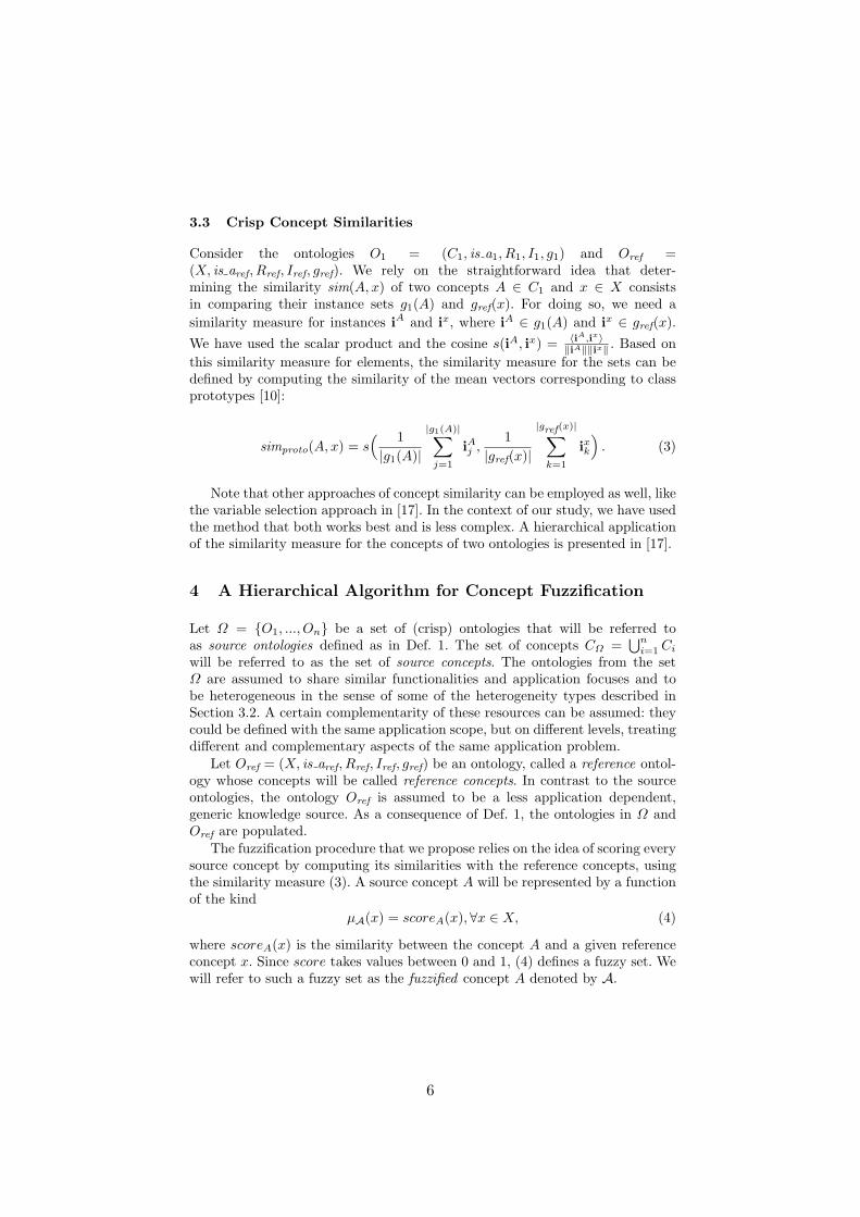
The fuzzification procedure that we propose relies on the idea of scoring everysource concept by computing its similarities with the reference concepts, usingthe similarity measure (3). A source concept A will be represented by a functionof the kind

µA(x) = scoreA(x),∀x ∈ X, (4)

where scoreA(x) is the similarity between the concept A and a given referenceconcept x. Since score takes values between 0 and 1, (4) defines a fuzzy set. Wewill refer to such a fuzzy set as the fuzzified concept A denoted by A.

6

In order to fuzzify the concepts of a source ontology O1, we propose thefollowing hierarchical algorithm. First, we assign score-vectors, i.e. fuzzy mem-bership functions to all leaf-node concepts of O1. Every non-leaf node, if it doesnot contain instances (documents) of its own, is scored as the maximum of thescores of its children for every x ∈ X. If a non-leaf node has directly assignedinstances (not inherited from its children), the node is first scored on the basis ofthese instances with respect to the reference ontology, and then as the maximumof its children and itself. To illustrate, let a concept A have children A′ and A′′

and let the non-empty function g∗(A) represent the instances assigned directlyto the concept A. We compute the following similarity scores for this conceptw.r.t. the set X :

scoreA(x) = maxscoreA′(x), scoreA′′(x), scoreg∗(A)(x),∀x ∈ X. (5)

Above, scoreg∗(A)(x) conventionally denotes the similarity obtained for the con-cept A and a reference concept x by only taking into account the documentsassigned directly to A. The algorithm is given in Alg. 1.

It is worth noting that assigning the max of all children to the parent forevery x leads to a convergence to uniformity of the membership functions fornodes higher up in the hierarchy. Naturally, the functions of the higher levelconcepts are expected to be less “specific” than those of the lower level concepts.A concept in a hierarchical structure can be seen as the union of its descendants,and a union corresponds to taking the max (an approach underlying the singlelink strategy used in clustering).

The hierarchical scoring procedure has the advantage that every x-score willbe larger for a parent node than those for any of its children, and it holdsthat µA′(x)→ µA(x) = 1 for all x and all children A′ of A. From computationalviewpoint, the procedure which only scores the populated nodes is less expensive,compared to scoring all nodes one by one.

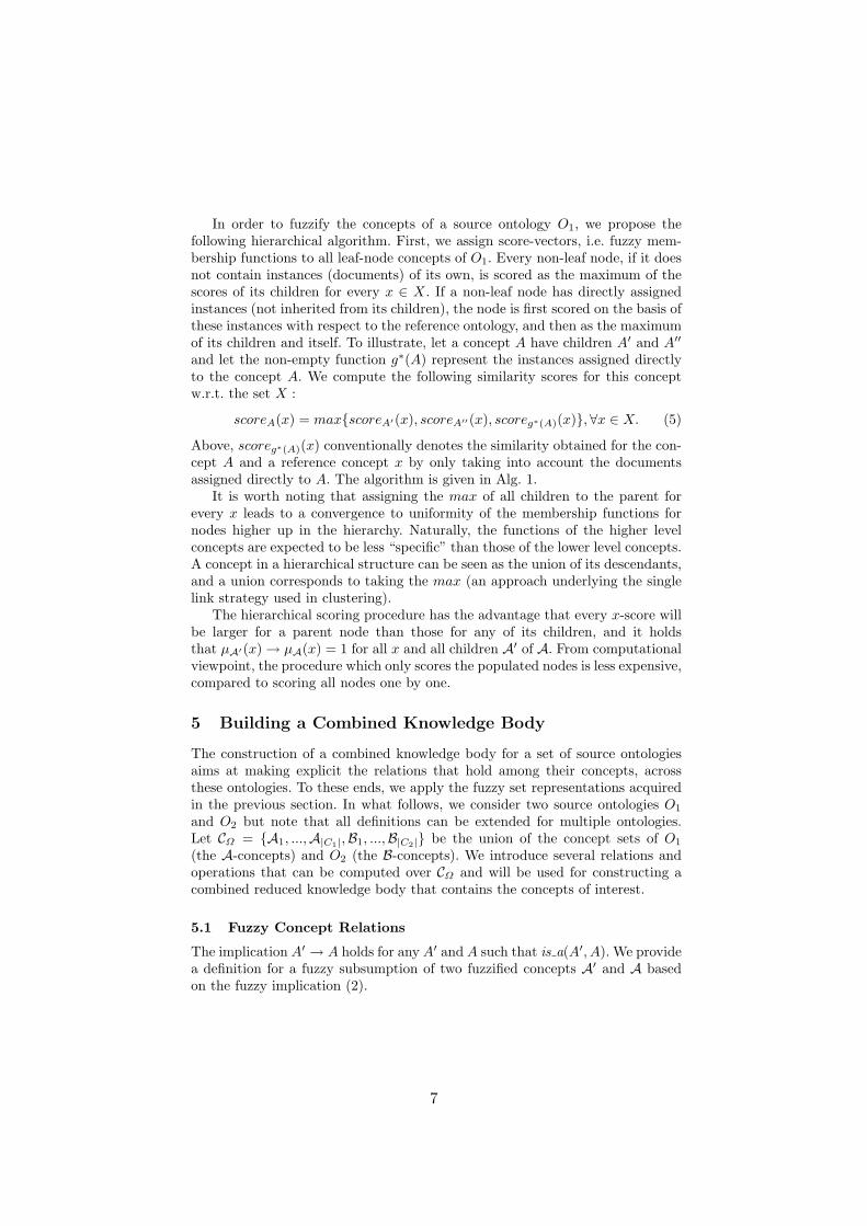
5 Building a Combined Knowledge Body

The construction of a combined knowledge body for a set of source ontologiesaims at making explicit the relations that hold among their concepts, acrossthese ontologies. To these ends, we apply the fuzzy set representations acquiredin the previous section. In what follows, we consider two source ontologies O1

and O2 but note that all definitions can be extended for multiple ontologies.Let CΩ = A1, ...,A|C1|,B1, ...,B|C2| be the union of the concept sets of O1

(the A-concepts) and O2 (the B-concepts). We introduce several relations andoperations that can be computed over CΩ and will be used for constructing acombined reduced knowledge body that contains the concepts of interest.

5.1 Fuzzy Concept Relations

The implication A′ → A holds for any A′ and A such that is a(A′, A). We providea definition for a fuzzy subsumption of two fuzzified concepts A′ and A basedon the fuzzy implication (2).

7

Function score(concept A, ontology Oref , sim. measure sim)begin

for i = 1, ..., |X| dosim[i] = sim(A, xi) // xi ∈ X

return simendProcedure hierachicalScoring(ontology O, ontology Oref , sim. measure sim)begin

1. Let C be the list of concepts in O.2. Let L be a list of nodes, initially empty3. Do until C is empty:

(a) Let L′ be the list of nodes in C that have only children in L(b) L = append(L, L′)(c) C = C − L′

4. Iterate over L (first to last), with A being the current element:if children(A) = ∅ thenscore(A) = score(A, Oref , sim)

elseif g∗(A) 6= ∅ then

score(A) = maxmaxB∈children(A)score(B), score(A, Oref , sim)else

score(A) = maxB∈children(A)score(B)

return score(A), ∀A ∈ Cend

Algorithm 1: An algorithm for hierarchical scoring of the source concepts.

Definition 2 (Fuzzy Subsumption). The subsumption A′ is a A is definedand denoted in the following manner:

is a(A′,A) = infx∈X

µA′→A(x) (6)

Equation (6) defines the fuzzy subsumption as a degree between 0 and 1 to whichone concept is the subsumer of another. It can be shown that is a, similarly toits crisp version, is reflexive and transitive (i.e. a quasi-order). In addition, thehierarchical procedure for concept fuzzification introduced in the previous sectionassures that is a(A′, A) = 1 holds for every child-parent concept pair, i.e. thecrisp subsumption relation is preserved by the fuzzification process.

Taking the example of a collaborative platform from the introduction, com-puting the fuzzy is a between two concepts allows for answering a user queryregarding generality and specificity of their partners concepts with respect to agiven target concept.

We provide a definition of a fuzzy ontology which follows directly from thefuzzification of the source concepts and their is a relations introduced above.

Definition 3 (Fuzzy Ontology). Let C be a set of (fuzzy) concepts, is a :C × C → [0, 1] a fuzzy is a-relationship, R a set of fuzzy relations on C, i.e., R

8

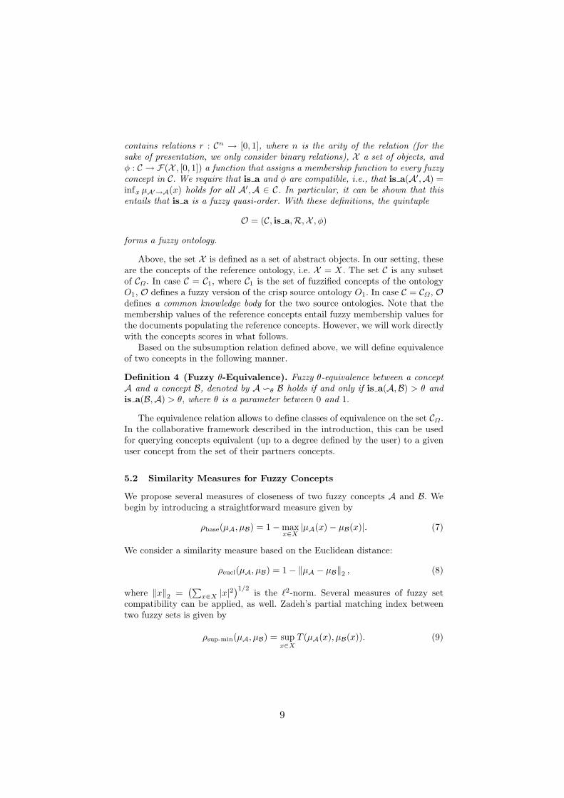
contains relations r : Cn → [0, 1], where n is the arity of the relation (for thesake of presentation, we only consider binary relations), X a set of objects, andφ : C → F(X , [0, 1]) a function that assigns a membership function to every fuzzyconcept in C. We require that is a and φ are compatible, i.e., that is a(A′,A) =infx µA′→A(x) holds for all A′,A ∈ C. In particular, it can be shown that thisentails that is a is a fuzzy quasi-order. With these definitions, the quintuple

O = (C, is a,R,X , φ)

forms a fuzzy ontology.

Above, the set X is defined as a set of abstract objects. In our setting, theseare the concepts of the reference ontology, i.e. X = X. The set C is any subsetof CΩ . In case C = C1, where C1 is the set of fuzzified concepts of the ontologyO1, O defines a fuzzy version of the crisp source ontology O1. In case C = CΩ , Odefines a common knowledge body for the two source ontologies. Note that themembership values of the reference concepts entail fuzzy membership values forthe documents populating the reference concepts. However, we will work directlywith the concepts scores in what follows.

Based on the subsumption relation defined above, we will define equivalenceof two concepts in the following manner.

Definition 4 (Fuzzy θ-Equivalence). Fuzzy θ-equivalence between a conceptA and a concept B, denoted by A vθ B holds if and only if is a(A,B) > θ andis a(B,A) > θ, where θ is a parameter between 0 and 1.

The equivalence relation allows to define classes of equivalence on the set CΩ .In the collaborative framework described in the introduction, this can be usedfor querying concepts equivalent (up to a degree defined by the user) to a givenuser concept from the set of their partners concepts.

5.2 Similarity Measures for Fuzzy Concepts

We propose several measures of closeness of two fuzzy concepts A and B. Webegin by introducing a straightforward measure given by

ρbase(µA, µB) = 1−maxx∈X|µA(x)− µB(x)|. (7)

We consider a similarity measure based on the Euclidean distance:

ρeucl(µA, µB) = 1− ‖µA − µB‖2 , (8)

where ‖x‖2 =(∑

x∈X |x|2)1/2 is the `2-norm. Several measures of fuzzy set

compatibility can be applied, as well. Zadeh’s partial matching index betweentwo fuzzy sets is given by

ρsup-min(µA, µB) = supx∈X

T (µA(x), µB(x)). (9)

9

Finally, the Jaccard coefficient is defined by

ρjacc(µA, µB) =∑x T (µA(x), µB(x))∑x S(µA(x), µB(x))

. (10)

It is required that at least one of the functions µA or µB takes a non-zero valuefor some x. T and S are as defined in Section 3.

The similarity measures listed above provide different information as com-pared to the relations introduced in the previous subsection. Subsumption andequivalence characterize the structural relation between concepts, whereas sim-ilarity measures closeness between set elements. The two types of informationare to be used in a complementary manner within the collaboration framework.

5.3 Quantifying Commonality and Relative Specificity

The union of two fuzzy concepts can be decomposed into three components,each quantifying, respectively, the commonality of both concepts, the specificityof the first compared to the second and the specificity of the second comparedto the first expressed in the following manner

S(A,B) = (AB) + (A− B) + (B −A). (11)

Each of these components is defined as follows and, respectively, accounts for:

AB = T (A,B) // what is common to both concepts; (12)A− B = T (A,¬B) // what is characteristic for A; (13)B −A = T (B,¬A) // what is characteristic for B. (14)

Several merge options can be provided to the user with respect to the valuesof these three components. In case AB is significantly larger than each of A−Band B−A, the two concepts can be merged into their union. In case one of A−Bor B −A is larger than the other two components, the concepts can be mergedto either A or B.

6 Experiments

We situate our experiments in the multimedia domain, opposing two comple-mentary heterogeneous ontologies containing annotated pictures. We chose, onone hand, LSCOM [14] initially built in the framework of TRECVID1 and pop-ulated with the development set of TRECVID 2005. Since this set containsimages from broadcast news videos, LSCOM is particularly adapted to anno-tate this kind of content, thus contains abstract and specific concepts (e.g. Sci-ence Technology, Interview On Location). On the other hand, we used

1 http://www-nlpir.nist.gov/projects/tv2005/

10

WordNet [11] populated with the LabelMe dataset [12], referred to as the La-belMe ontology. Contrarily to LSCOM, this ontology is very general, populatedwith photographs from daily life and contains concepts such as car, computer,person, etc. The parts of the two multimedia ontologies used in the experimentsare shown in Figure 1.

Fig. 1. The LSCOM (left) and the LabelMe (right) ontologies.

Fig. 2. The LSCOM concept Bus: a visual and a textual instance.

A text document has been generated for every image of the two ontologies,by taking the names of all concepts that an image contains in its annotation,as well as the (textual) definitions of these concepts (the LSCOM definitions for

11

TRECVID images or the WordNet glosses for LabelMe images). An example of avisual instance of a multimedia concept and the constructed textual descriptionis given in Figure 2. Several problems related to this representation are worthnoting. The LSCOM keyword descriptions sometimes depend on negation andexclusion which are difficult to handle in a simple bag-of-words approach. Takingthe WordNet glosses of the terms in LabelMe introduces problems related topolysemy and synonymy. Additionally, a scene often consists of several objects,which are frequently not related to the object that determines the class of theimage. In such cases, the other objects in the image act as noise.

Concept A: LSCM:truck vs. LSCM:sports vs. LM:computer vs. LM:animal vs.Concept B: LSCM:gr.vehicle LSCM:basketball LM:elec. device LM:bird

is a(A,B) 1 0.007 1 0.004is a(B,A) 0.012 1 0.011 1is amean(A,B) 1 0.052 1 0.062is amean(B,A) 0.326 1 0.07 1

Base Sim. 0.848 0.959 0.915 0.390Eucl. Sim. 0.835 0.908 0.854 0.350SupMin Sim. 0.435 0.545 0.359 0.309Jacc. Sim. 0.870 0.814 0.733 0.399Cosine Sim. 0.974 0.994 0.975 0.551

Concept A: LM:gondola vs. LSCM:group vs. LSCM:truck vs. LSCM:truck vs.Concept B: LSCM:boat ship LM:audience LM:vehicle LM:conveyance

is a(A,B) 0.016 0.006 0.022 0.022is a(B,A) 0.009 1 0.012 0.012is amean(A,B) 0.86 0.022 0.748 0.769is amean(B,A) 0.167 1 0.301 0.281

Base Sim. 0.72 0.78 0.58 0.58Eucl. Sim. 0.66 0.71 0.40 0.38SupMin Sim. 0.069 0.082 0.22 0.22Jacc. Sim. 0.49 0.42 0.54 0.52Cosine Sim. 0.69 0.82 0.66 0.67

Table 1. Examples of pairs of matched intra-ontology concepts (above) and cross-ontology concepts (below), column-wise.

In order to fuzzify our source concepts, we have applied the hierarchicalscoring algorithm from Section 4 independently for each of the source ontologies.As a reference ontology, we have used an extended version of the Wikipedia’s so-called main topic classifications (adding approx. 3 additional concepts to everyfirst level class), containing more than 30 categories. For each topic category, weincluded a set of corresponding documents from the Inex 2007 corpus.

The new combined knowledge body has been constructed by first taking theunion of all fuzzified source concepts. For every pair of concepts, we have com-puted their Godel subsumptional relations, as well as the degree of their similar-

12

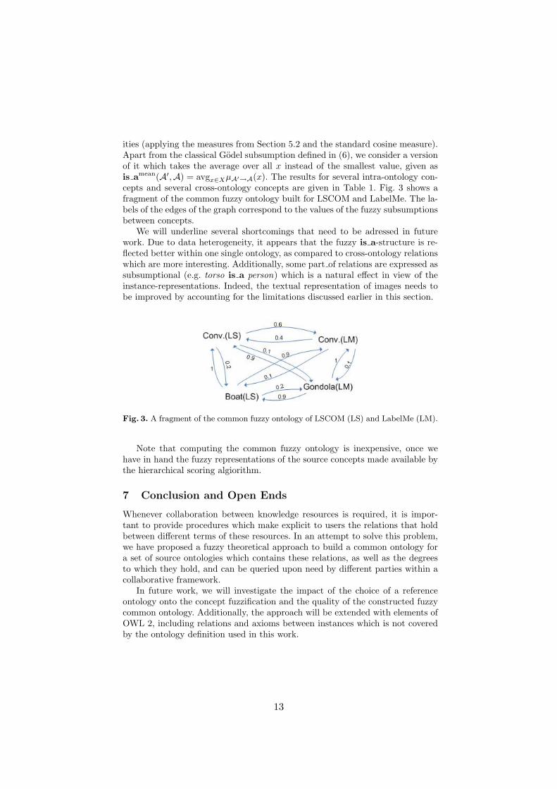
ities (applying the measures from Section 5.2 and the standard cosine measure).Apart from the classical Godel subsumption defined in (6), we consider a versionof it which takes the average over all x instead of the smallest value, given asis amean(A′,A) = avgx∈XµA′→A(x). The results for several intra-ontology con-cepts and several cross-ontology concepts are given in Table 1. Fig. 3 shows afragment of the common fuzzy ontology built for LSCOM and LabelMe. The la-bels of the edges of the graph correspond to the values of the fuzzy subsumptionsbetween concepts.

We will underline several shortcomings that need to be adressed in futurework. Due to data heterogeneity, it appears that the fuzzy is a-structure is re-flected better within one single ontology, as compared to cross-ontology relationswhich are more interesting. Additionally, some part of relations are expressed assubsumptional (e.g. torso is a person) which is a natural effect in view of theinstance-representations. Indeed, the textual representation of images needs tobe improved by accounting for the limitations discussed earlier in this section.

Fig. 3. A fragment of the common fuzzy ontology of LSCOM (LS) and LabelMe (LM).

Note that computing the common fuzzy ontology is inexpensive, once wehave in hand the fuzzy representations of the source concepts made available bythe hierarchical scoring algiorithm.

7 Conclusion and Open Ends

Whenever collaboration between knowledge resources is required, it is impor-tant to provide procedures which make explicit to users the relations that holdbetween different terms of these resources. In an attempt to solve this problem,we have proposed a fuzzy theoretical approach to build a common ontology fora set of source ontologies which contains these relations, as well as the degreesto which they hold, and can be queried upon need by different parties within acollaborative framework.

In future work, we will investigate the impact of the choice of a referenceontology onto the concept fuzzification and the quality of the constructed fuzzycommon ontology. Additionally, the approach will be extended with elements ofOWL 2, including relations and axioms between instances which is not coveredby the ontology definition used in this work.

13

References

1. J.-I. Akahani, K. Hiramatsu, and T. Satoh. Approximate query reformulationbased on hierarchical ontology mapping. In In Proc. of Intl Workshop on SWFAT,pages 43–46, 2003.

2. A. Bahri, R. Bouaziz, and F. Gargouri. Dealing with similarity relations in fuzzyontologies. In Fuzzy Systems Conference, 2007. FUZZ-IEEE 2007. IEEE Interna-tional, pages 1–6. IEEE, 2007.

3. P. Buche, J. Dibie-Barthelemy, and L. Ibanescu. Ontology mapping using fuzzyconceptual graphs and rules. In ICCS Supplement, pages 17–24, 2008.

4. S. Calegari and D. Ciucci. Fuzzy ontology, fuzzy description logics and fuzzy-owl.In WILF, pages 118–126, 2007.

5. S. Calegari and E. Sanchez. A fuzzy ontology-approach to improve semantic infor-mation retrieval. In URSW, 2007.

6. V. Cross and X. Yu. A fuzzy set framework for ontological similarity measures. InWCCI 2010, FUZZ-IEEE 2010, pages 1 – 8. IEEE Compter Society Press, 2010.

7. J. Euzenat and P. Shvaiko. Ontology Matching. Springer-Verlag, 1 edition, 2007.8. A. Ferrara, D. Lorusso, G. Stamou, G. Stoilos, V. Tzouvaras, and T. Venetis.

Resolution of conflicts among ontology mappings: a fuzzy approach. OM’08 atISWC, 2008.

9. A. Gal and P. Shvaiko. Advances in web semantics i. chapter Advances in OntologyMatching, pages 176–198. Springer-Verlag, Berlin, Heidelberg, 2009.

10. M. S. Lacher and G. Groh. Facilitating the exchange of explicit knowledge throughontology mappings. In Proceedings of the 14th FLAIRS Conf., pages 305–309.AAAI Press, 2001.

11. G.A. Miller. WordNet: a lexical database for English. Communications of theACM, 38(11):39–41, 1995.

12. B.C. Russell, A. Torralba, K.P. Murphy, and W.T. Freeman. Labelme: A databaseand web-based tool for image annotation. International Journal of Computer Vi-sion, 77(1), 2008.

13. E. Sanchez and T. Yamanoi. Fuzzy ontologies for the semantic web. Flexible QueryAnswering Systems, pages 691–699, 2006.

14. J.R. Smith and S.F. Chang. Large-scale concept ontology for multimedia. IEEEMultimedia, 13(3):86 – 91, 2006.

15. U. Straccia. Towards a fuzzy description logic for the semantic web (preliminaryreport). In Asuncin Gomez-Perez and Jrme Euzenat, editors, The Semantic Web:Research and Applications, volume 3532 of Lecture Notes in Computer Science,pages 73–123. Springer Berlin / Heidelberg, 2005.

16. H. Stuckenschmidt. Approximate information filtering on the semantic web. InM. Jarke, G. Lakemeyer, and J. Koehler, editors, KI 2002, volume 2479 of LNCS,pages 195–228. Springer Berlin / Heidelberg, 2002.

17. K. Todorov, P. Geibel, and K.-U. Khnberger. Mining concept similarities for het-erogeneous ontologies. In P. Perner, editor, Advances in Data Mining. Applicationsand Theoretical Aspects, volume 6171 of LNCS, pages 86–100. Springer Berlin /Heidelberg, 2010.

18. B. Xu, D. Kang, J. Lu, Y. Li, and J. Jiang. Mapping fuzzy concepts between fuzzyontologies. In R. Khosla, R. J. Howlett, and L. C. Jain, editors, Knowledge-BasedIntelligent Information and Engineering Systems, volume 3683 of Lecture Notes inComputer Science, pages 199–205. Springer Berlin / Heidelberg, 2005.

19. L.A. Zadeh. Fuzzy sets. Information and Control, 8(3):338 – 353, 1965.

14

Estimating Uncertainty of Categorical Web Data

Davide Ceolin, Willem Robert van Hage, Wan Fokkink, and Guus Schreiber

VU University AmsterdamDe Boelelaan 1081a

1081HV Amsterdam, The Netherlandsd.ceolin,w.r.van.hage,w.j.fokkink,guus.schreiber@vu.nl

Abstract. Web data often manifest high levels of uncertainty. We focuson categorical Web data and we represent these uncertainty levels asfirst or second order uncertainty. By means of concrete examples, weshow how to quantify and handle these uncertainties using the Beta-Binomial and the Dirichlet-Multinomial models, as well as how take intoaccount possibly unseen categories in our samples by using the DirichletProcess.

Keywords: Uncertainty, Bayesian statistics, Non-parametric statistics,Beta-Binomial, Dirichlet-Multinomial, Dirichlet Process

1 Introduction

The World Wide Web and the Semantic Web offer access to an enormous amountof data and this is one of their major strengths. However, the uncertainty aboutthese data is quite high, due to the multi-authoring nature of the Web itself andto its time variability: some data are accurate, some others are incomplete orinaccurate, and generally, such a reliability level is not explicitly provided.

We focus on the real distribution of these Web data, in particular of cate-gorical Web data, regardless of whether they are provided by documents, RDF(see [27]) statements or other means. Categorical data are the among the mostimportant types of Web data, because they include also URIs. We do not look forcorrelations among data, but we stick to estimating how category proportionsdistribute over populations of Web data.

We assume that any kind of reasoning that might produce new statements(e.g. subsumption) has already taken place. Hence, unlike for instance Fukuoeet al. (see [10]), that apply probabilistic reasoning in parallel to OWL (see [26])reasoning, we will propose some models to address uncertainty issues on topof that kind of reasoning layers. These models, namely the parametric Beta-Binomial and Dirichlet-Multinomial, and the non-parametric Dirichlet Process,will use first and second order probabilities and the generation of new classes ofobservations, to derive safe conclusions on the overall populations of our data,given that we are deriving those from possibly biased samples.

First we will describe the scope of these models (section 2), second we willintroduce the concept of conjugate prior (section 3), and then two classes of

15

models: parametric (section 4) and non-parametric (section 5). Finally we willdiscuss the results and provide conclusions (section 6).

2 Scope of this work

2.1 Empirical evidence from the WebUncertainty is often an issue in case of empirical data. This is especially the casewith empirical Web data, because the nature of the Web increases the relevanceof this problem but also offers means to address it, as we will see in this section.The relevance of the problem is related to the utilization of the mass of data thatany user can find over the network: can one safely make use of these data? Lotsof data are provided on the Web by entities the reputation of which is not surelyknown. In addition to that, the fact that we access the Web by crawling, meansthat we should reduce our uncertainty progressively, as long as we increment ourknowledge. Moreover, when handling our samples it is often hard to determinehow representative such a sample is of the entire population, since often we donot own enough sure information about it.

On the other hand, the huge amount of Web data gives also a solution formanaging this reliability issue, since it can hopefully provide the evidence nec-essary to limit the risk when using a certain data set.

Of course, even within the Web it can be hard to find multiple sources as-serting about a given fact of interest. However, the growing dimension of theWeb makes it reasonable to believe in the possibility to find more than one dataset about the given focus, at least by means of implicit and indirect evidence.

This work aims showing how it is possible to address the described issues byhandling such empirical data, categorical empirical data in particular, by meansof the Beta-Binomial, Dirichlet-Multinomial and Dirichlet Process models.

2.2 RequirementsOur approach will need to be quite elastic in order to cover several issues, asdescribed below. The non-triviality of the problem comes in a large part fromthe impossibility to directly handle the sampling process from which we deriveour conclusions. The requirements that we will need to meet are:Ability to handle incremental data acquisition The model should be in-

cremental, in order to reflect the process of data acquisition: as long as wecollect more data (even by crawling), our knowledge will reflect that increase.

Prudence It should derive prudent conclusions given all the available informa-tion. In case not enough information is available, the wide range of possibleconclusions derivable will clearly make it harder to set up a decision strategy.

Cope with biased sampling The model should deal with the fact that we arenot managing a supervised experiment, that is, we are not randomly sam-pling from the population. We are using an available data set to derive safeconsequences, but these data could, in principle, be incomplete, inaccurateor biased, and we must take this into account.

16

Ability to handle samples from mixtures of probability distributionsThe data we have at our disposal may have been drawn from diverse distri-butions, so we can’t use the central limit theorem, because it relies on thefact that the sequence of variables is identically distributed. This implies theimpossibility to make use of estimators that approximate by means of theNormal distribution.

Ability to handle temporal variability of parameters Data distributionscan change over time, and this variability has to be properly accounted.

Complementarity with higher order layers The aim of the approach is toquantify the intrinsic uncertainty in the data provided by the reasoning layer,and, in turn, to provide to higher order layers (time series analysis, decisionstrategy, trust, etc.) reliable data and/or metadata.

2.3 Related work

The models adopted here are applied in a variety of fields. For the parametricmodels, examples of applications are: topic identification and document cluster-ing (see [18, 6]), quantum physics (see [15]), and combat modeling in the navaldomain (see [17]). What these heterogeneous fields have in common is the pres-ence of multiple levels of uncertainty (for more details about this, see sect. 4).

Also non-parametric models are applied in a wide variety of fields. Examplesof these applications include document classification [3] and haplotype inference[30]. These heterogeneous fields have in common with the previous applicationthe presence of several layers of uncertainty, but they also show lack of priorinformation about the number of parameters. These concepts will be treated insection 5 where even the Wilcoxon sign-ranked test (see [29]), used for validationpurposes, falls into the non-parametric models class.

As to our knowledge, the chosen models have not been applied to categoricalWeb data yet. We propose to adopt them, because, as the following sections willshow, they fit the requirements previously listed.

3 Prelude: Conjugate priors

To tackle the requirements described in the previous section, we adopt somebayesian parametric and non-parametric models in order to be able to answerquestions about Web data.

Conjugate priors (see [12]) are the “leit motiv”, common to all the modelsadopted here. The basic idea starts from the Bayes theorem (1): given a priorknowledge and our data, we update the knowledge into a posterior probability.

P (A|B) = P (B|A) ∗ P (A)P (B) (1)

This theorem describes how it is possible to compute the posterior probability,P (A|B), given the prior probability of our data, P (A), the likelihood of themodel, given the data, P (B|A), and the probability of the model itself, P (B).

17

When dealing with continuous probability distributions, the computation ofthe posterior distribution by means of Bayes theorem can be problematic, due tothe need to possibly compute complicated integrals. Conjugate priors allow usto overcome this issue: when prior and posterior probability distributions belongto the same exponential family, the posterior probability can be obtained byupdating the prior parameters with values depending on the observed sample(see also [9]). Exponential families are classes of probability distributions havingtheir density functions sharing the form f(x) = ea(q)b(x)+c(q)+d(x), with q aknown parameter and a, b, c, d known functions. Exponential families includemany important probability distributions, like the Normal, Binomial, Beta, etc.,see [5]. So, if X is a random variable that distributes as defined by the functionP (p) (for some parameter or vector of parameters p) and, in turn, p distributes asQ(α) for some parameter (or vector of parameters) α called “hyperparameter”),and P belongs to the same exponential family as Q,

p ∼ Q(α), X ∼ P (p)then, after having observed obs,

p ∼ Q(α′)where α′ = f(α, obs), for some function f . For example, the Beta distributionis the conjugate of the Binomial distribution. This means that the Beta, shapedby the prior information and by the observations, defines the range within whichthe parameter p of the Binomial will probably be situated, instead of directlyassigning to it the most likely value. Other examples of conjugate priors are:Dirichlet, which is conjugate to the Multinomial, and Gaussian, which is conju-gate to itself.

Conjugacy guarantees ease of computation, which is a desirable characteristicwhen dealing with very big data sets as Web data sets often are. Moreover, themodel is incremental, and this makes it fit the crawling process with whichWeb data are obtained, because crawling, in turn, is an incremental process.Both the heterogeneity of the Web and the crawling process itself increase theuncertainty of Web data. The probabilistic determination of the parameters ofthe distributions adds a smoothing factor that helps to handle this uncertainty.

4 Parametric bayesian models for categorical Web dataIn this section we will handle situations where the number of categories is knowna priori, by using the Dirichlet-Multinomial model and its special case with twocategories, i.e. the Beta-Binomial model [9]. As generalized versions of the Bino-mial and Multinomial distribution, they describe the realization of sequences ofmutually exclusive events. Categorical data can be seen as examples of such se-quences. These models are parametric, since the number and type of parametersis given a priori, and they can also be classified as “empirical bayesian models”.This further classification means that they can be seen as an approximation ofa full hierarchical bayesian model, where the prior hyperparameters are set totheir maximum likelihood values according to the analyzed sample.

18

4.1 Case study 1: Deciding between alternatives - ratio estimation

Suppose that a museum has to annotate a particular item I of its collection.Suppose further, that the museum does not have expertise in the house aboutthat particular subject and, for this reason, in order to correctly classify theitem, it seeks judgments from outside people, in particular from Web users thatprovide evidence of owning the desired expertise.

After having collected judgements, the museum faces two possible classifica-tions for the item, C1 and C2. C1 is supported by four experts, while C2 by onlyone expert. We can use these numbers to estimate a probability distribution thatresembles the correct distribution of C1 and C2 among all possible annotations.

A basic decision strategy that could make use of this probability distribu-tion, could accept a certain classification only if its probability is greater orequal to a given threshold (e.g. 0.75). If so, the Binomial distribution repre-senting the sample would be treated as representative of the population, andthe sample proportions would be used as parameters of a Bernoulli distributionabout the possible classifications for the analyzed item: P (class(I) = C1) =4/5 = 0.8, P (class(I) = C2) = 1/5 = 0.2. (A Bernoulli distribution describesthe possibility that one of two alternative events happens. One of these eventshappens with probability p, the other one with probability 1 − p. A Binomialdistribution with parameters n, p represents the outcome of a sequence of nBernoulli trials having all the same parameter p.)

However, this solution shows a manifest leak. It provides to the decisionstrategy layer the probabilities for each of the possible outcomes, but theseprobabilities are based on the current available sample, with the assumptionthat it correctly represents the complete population of all existing annotations.This assumption is too ambitious. (Flipping a coin twice, obtaining a heads anda tails, does not guarantee that the coin is fair, yet.)

In order to overcome such a limitation, we should try to quantify how muchwe can rely on the computed probability. In other words, if the previously com-puted probability can be referred as a “first order” probability, what we need tocompute now is a “second order” probability (see [15]). Given that the conjugateprior for the Binomial distribution representing our data is the Beta distribution,the model becomes:

p ∼ Beta(α, β), X ∼ Bin(p, n) (2)

where α = #evidenceC1 + 1 and β = #evidenceC2 + 1.By analyzing the shape of the conjugate prior Beta(5,2), we can be certain

enough about the probability of C1 being safely above our acceptance threshold.In principle, our sample could be drawn by a population distributed with a40%−60% proportion. If so, given the threshold of acceptance of 0.75, we wouldnot be able to take a decision based on the evidence. However, the quantificationof that proportion would only be possible if we know the population. Given thatwe do not have such information, we need to estimate it, by computing (3), wherewe can see how the probability of the parameter p being above the threshold isless than 0.5. This manifests the need for more evidence: our sample suggests to

19

accept the most popular value, but the sample itself does not guarantee to berepresentative enough of the population.

P (p ≥ 0.75) = 0.4660645, p ∼ Beta(5, 2) (3)

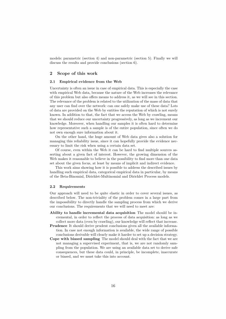
Table 1 shows how the confidence in the value p being above the threshold growsas long as we increase the size of the sample, when the proportion is kept. By ap-plying the previous strategy (0.75 threshold) also to the second order probability,we will still choose C1, but only if supported by a sample of size at least equal to15.

Table 1: The proportion withinthe sample is kept, so the mostlikely value for p is always exactlythat ratio. However, given our 0.75threshold, we are sure enough onlyif the sample size is 15 or higher.

#C1 #C2 P (p ≥ 0.75)p ∼ Beta(#C1 + 1,#C2 + 1)

4 1 0.46606458 2 0.544799112 3 0.8822048

0.0

0.1

0.2

0.3

0.4

0.5

Positive outcomes

P(X

)

0 1 2 3 4 5 6

Binomial(5,0.8)Beta−Binomial(5,5,2)Beta−Binomial(5,9,3)Beta−Binomial(5,13,4)

Fig. 1: Comparison between Binomialand Beta-Binomial with increasing sam-ple size. As the sample size grows, Beta-Binomial approaches Binomial.

Finally, these considerations couldalso be done on the basis of theBeta-Binomial distribution, which isa probability distribution represent-ing a Binomial which parameter p israndomly drawn from a Beta distribu-tion. The Beta-Binomial summarizesmodel (2) in one single function (4).We can see from Table 2 that the ex-pected proportion of the probabilitydistribution approaches the ratio ofthe sample (0.8), as the sample sizegrows. If so, the sample is regarded asa better representative of the entirepopulation and the Beta-Binomial, assample size grows, will converge to theBinomial representing the sample (seeFig. 1).

X ∼ BetaBin(n, α, β) = p ∼ Beta(α, β), X ∼ Bin(n, p) (4)

4.2 Case study 2: deciding proportions - confidence intervalsestimation

The Linked Open Piracy1 is a repository of piracy attacks that happened aroundthe world in the period 2005 - 2011, derived from reports retrieved from the ICC-1 http://semanticweb.cs.vu.nl/lop

20

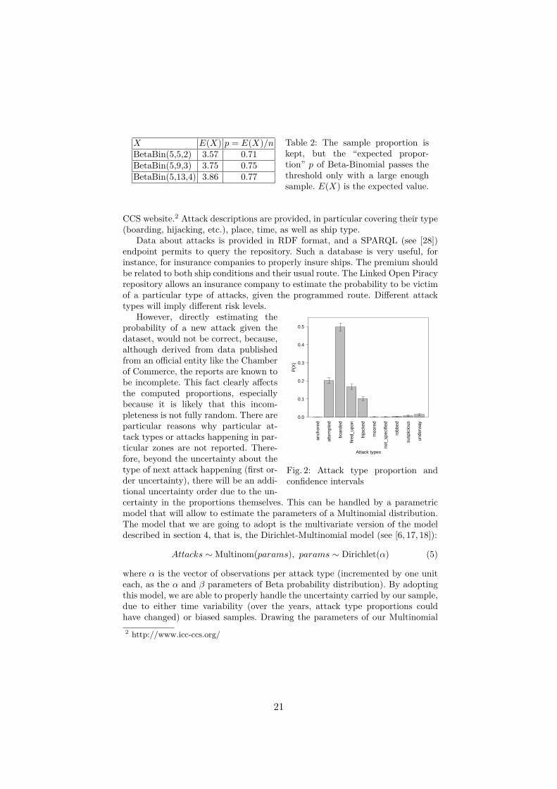
X E(X) p = E(X)/nBetaBin(5,5,2) 3.57 0.71BetaBin(5,9,3) 3.75 0.75BetaBin(5,13,4) 3.86 0.77

Table 2: The sample proportion iskept, but the “expected propor-tion” p of Beta-Binomial passes thethreshold only with a large enoughsample. E(X) is the expected value.

CCS website.2 Attack descriptions are provided, in particular covering their type(boarding, hijacking, etc.), place, time, as well as ship type.

Data about attacks is provided in RDF format, and a SPARQL (see [28])endpoint permits to query the repository. Such a database is very useful, forinstance, for insurance companies to properly insure ships. The premium shouldbe related to both ship conditions and their usual route. The Linked Open Piracyrepository allows an insurance company to estimate the probability to be victimof a particular type of attacks, given the programmed route. Different attacktypes will imply different risk levels.

anch

ored

atte

mpt

ed

boar

ded

fired

_upo

n

hija

cked

moo

red

not_

spec

ified

robb

ed

susp

icio

us

unde

rway

P(X

)

0.0

0.1

0.2

0.3

0.4

0.5

Attack types

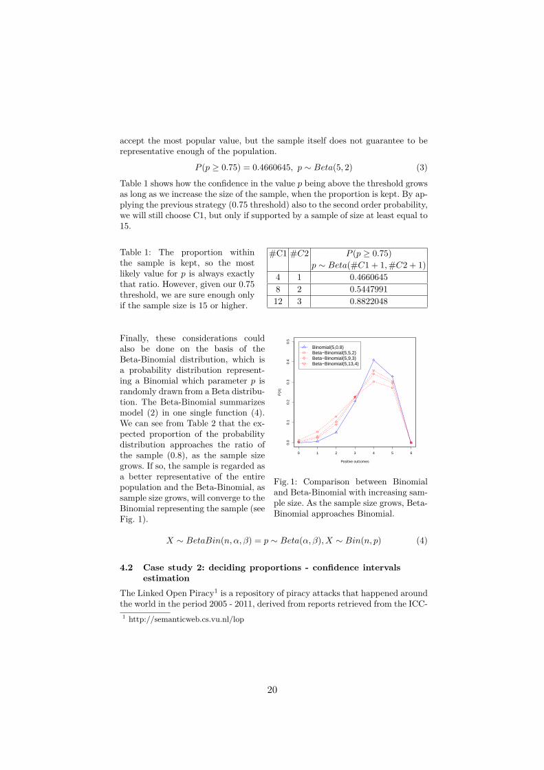
Fig. 2: Attack type proportion andconfidence intervals

However, directly estimating theprobability of a new attack given thedataset, would not be correct, because,although derived from data publishedfrom an official entity like the Chamberof Commerce, the reports are known tobe incomplete. This fact clearly affectsthe computed proportions, especiallybecause it is likely that this incom-pleteness is not fully random. There areparticular reasons why particular at-tack types or attacks happening in par-ticular zones are not reported. There-fore, beyond the uncertainty about thetype of next attack happening (first or-der uncertainty), there will be an addi-tional uncertainty order due to the un-certainty in the proportions themselves. This can be handled by a parametricmodel that will allow to estimate the parameters of a Multinomial distribution.The model that we are going to adopt is the multivariate version of the modeldescribed in section 4, that is, the Dirichlet-Multinomial model (see [6, 17, 18]):

Attacks ∼ Multinom(params), params ∼ Dirichlet(α) (5)

where α is the vector of observations per attack type (incremented by one uniteach, as the α and β parameters of Beta probability distribution). By adoptingthis model, we are able to properly handle the uncertainty carried by our sample,due to either time variability (over the years, attack type proportions couldhave changed) or biased samples. Drawing the parameters of our Multinomial2 http://www.icc-ccs.org/

21

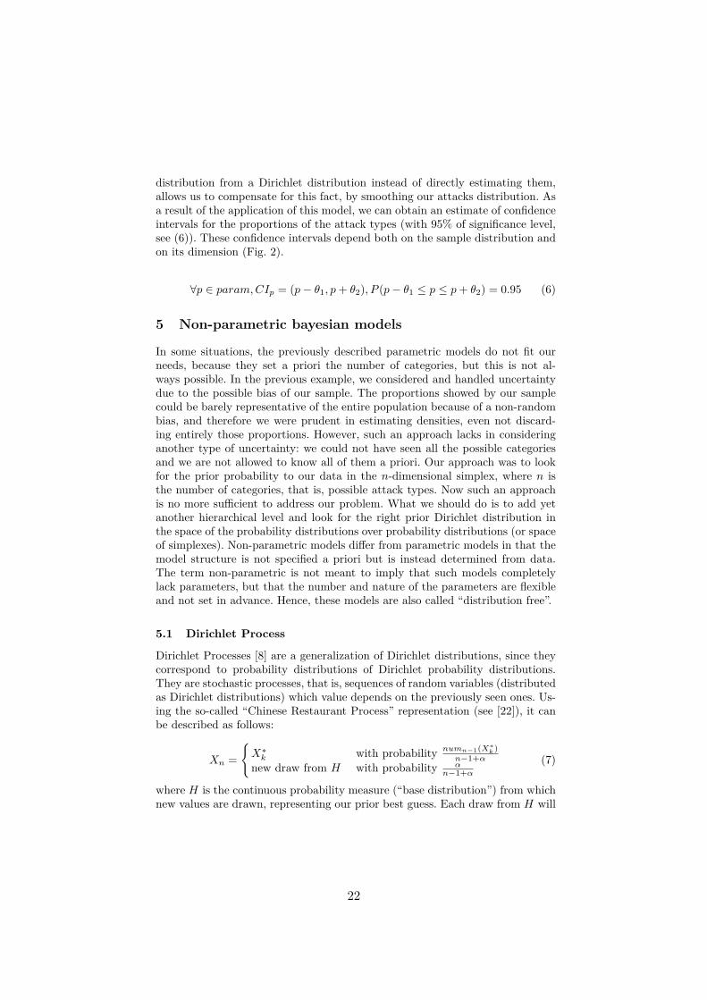
distribution from a Dirichlet distribution instead of directly estimating them,allows us to compensate for this fact, by smoothing our attacks distribution. Asa result of the application of this model, we can obtain an estimate of confidenceintervals for the proportions of the attack types (with 95% of significance level,see (6)). These confidence intervals depend both on the sample distribution andon its dimension (Fig. 2).

∀p ∈ param,CIp = (p− θ1, p+ θ2), P (p− θ1 ≤ p ≤ p+ θ2) = 0.95 (6)

5 Non-parametric bayesian models

In some situations, the previously described parametric models do not fit ourneeds, because they set a priori the number of categories, but this is not al-ways possible. In the previous example, we considered and handled uncertaintydue to the possible bias of our sample. The proportions showed by our samplecould be barely representative of the entire population because of a non-randombias, and therefore we were prudent in estimating densities, even not discard-ing entirely those proportions. However, such an approach lacks in consideringanother type of uncertainty: we could not have seen all the possible categoriesand we are not allowed to know all of them a priori. Our approach was to lookfor the prior probability to our data in the n-dimensional simplex, where n isthe number of categories, that is, possible attack types. Now such an approachis no more sufficient to address our problem. What we should do is to add yetanother hierarchical level and look for the right prior Dirichlet distribution inthe space of the probability distributions over probability distributions (or spaceof simplexes). Non-parametric models differ from parametric models in that themodel structure is not specified a priori but is instead determined from data.The term non-parametric is not meant to imply that such models completelylack parameters, but that the number and nature of the parameters are flexibleand not set in advance. Hence, these models are also called “distribution free”.

5.1 Dirichlet Process

Dirichlet Processes [8] are a generalization of Dirichlet distributions, since theycorrespond to probability distributions of Dirichlet probability distributions.They are stochastic processes, that is, sequences of random variables (distributedas Dirichlet distributions) which value depends on the previously seen ones. Us-ing the so-called “Chinese Restaurant Process” representation (see [22]), it canbe described as follows:

Xn =X∗k with probability numn−1(X∗k)

n−1+αnew draw from H with probability α

n−1+α(7)

where H is the continuous probability measure (“base distribution”) from whichnew values are drawn, representing our prior best guess. Each draw from H will

22

return a different value with probability 1. α is an aggregation parameter, inverseof the variance: the higher α, the smaller the variance, which can be interpretedas the confidence value in the base distribution H: the higher the α value is,the more the Dirichlet Process resembles H. The lower the α is, the more thevalue of the Dirichlet Process will tend to the value of the empirical distributionobserved. Each realization of the process is discrete and is equivalent to a drawfrom a Dirichlet distribution, because, if

G ∼ DP (H,α) (8)

is a Dirichlet Process, and Bni=1 are partitions of S, we have that

(G(B1)...G(Bn)) ∼ Dirichlet(αH(B1)...αH(Bn)) (9)

If our prior Dirichlet Process is (8), given (9) and the conjugacy betweenDirichlet and Multinomial distribution, our posterior Dirichlet Process (afterhaving observed n values θi) can be represented as one of the following tworepresentations:

(G(B1)...G(Bn))|θ1...θn ∼ Dirichlet(αH(B1) + nθ1 ...αH(Bn) + nθn) (10)

G | θ1...θn ∼ DP(α+ n,

α

α+ nH + n

α+ n

Σni=1δθin

)(11)

where δθi is the Dirac delta function (see [4]), that is, the function having densityonly in θi. The new base function will therefore be a merge of the prior H andthe empirical distribution, represented by means of a sum of Dirac delta’s. Theinitial status of a Dirichlet Process posterior to n observations, is equivalent tothe nth status of the initial Dirichlet Process that produced those observations(see De Finetti theorem, [13]).

The Dirichlet process, starting from a (possibly non-informative) “best guess”,as long as we collect more data, will approximate the real probability distribu-tion. Hence, it will correctly represent the population in a prudent (smoothed)way, exploiting conjugacy like the Dirichlet-Multinomial model, that approxi-mates well the real Multinomial distribution only with a large enough data set(see section 4). The improvement of the posterior base distribution is testifiedby the increase of the α parameter, proportional to the number of observations.

5.2 Case study 3: Classification of piracy attacks - unseen typesgeneration

We aim at predicting the type distributions of incoming attack events. In orderto build an “infinite category” model, we need to allow for event types to berandomly drawn from an infinite domain. Therefore, we map already observedattack types with random numbers in [0..1] and, since all events are a prioriequally likely, then new events will be drawn from the Uniform distribution,U(0, 1), that is our base distribution (and is a measure over [0..1]). The modelthen is:

23

– type1 ∼ DP (U(0, 1), α): the prior over the first attack type in region R;– attack1 ∼ Categorical(type1): type of the first attack in R during yeary.

After having observed attack1...n during yeary, our posterior process becomes:

typen+1 | attack1...n ∼ DP(α+ n,

α

α+ nU(0, 1) + n

α+ n

Σni=1δattacki

n

)

where α is a low value, given the low confidence in U(0, 1), and typen+1 is theprior of attackn+1, that happens during yeary+1. A Categorical distribution isa Bernoulli distribution with more than two possible outcomes (see Section 4).

Results Focusing on each region at time, we simulate all the attacks that hap-pened there in yeary+1. Names of new types generated by simulation are matchedto the actual yeary+1 names, that do not occur in yeary, in order of decreasingprobability. The simulation is compared with a projection of the proportions ofyearn over the actual categories of yearn+1. The comparison is made by measur-ing the distance of our simulation and of the projection from the real attack typesproportions of yeary+1 using the the Manhattan distance (see [16]). This metricsimply sums, for each attack type, the difference between the real yeary+1 prob-ability and the one we forecast. Hence, it can be regarded as an error measure.Table 3 summarizes the results over the entire dataset.3 Our simulation reducesthe distance (i.e. the error) with respect to the projection, as confirmed by aWilcoxon signed-rank test [29] at 95% significance level. (This non-parametricstatistical hypothesis test is used to determine whether one of the means of thepopulation of two samples is smaller/greater than the other.) The simulationimproves when large amount of data is available and the category cardinalityvaries, as in case of Region India, which results are reported in Fig. 3 and 4a.

Table 3: Averages and variances ofthe error of the two forecasts. Thesimulation gets a better performance.

Simulation ProjectionAverage distance 0.29 4 0.35Variance 0.09 4 0.21

0.0

0.2

0.4

0.6

0.8

(a) Year 2005

0.0

0.2

0.4

0.6

0.8

(b) Simulation

0.0

0.2

0.4

0.6

0.8

(c) Year 2006

attemptedboardedhijackedrobbed

Fig. 3: Comparison between the projection forecast and the simulation forecastwith the real-life year 2006 data of region India.

3 The code can be retrieved at http://www.few.vu.nl/~dceolin/DP/Dir.R

24

0.0

0.2

0.4

0.6

0.8

Years

Man

hatta

n di

stan

ces

projectedsimulated

2006 2007 2008 2009 2010

(a) ErrorsOverall dataset (each bar is one year of a region)

−2−1

01

2 Projection better than Simulation

Simulation better than Projection

Middle EastIndiaIndonesiaCaribbeanSouth East AsiaSouth AmericaEast AsiaWest AfricaGulf of AdenEast AfricaEuropeNorth America

20052006

20062007

20072008

20092010

20082009

(b) Distances differences

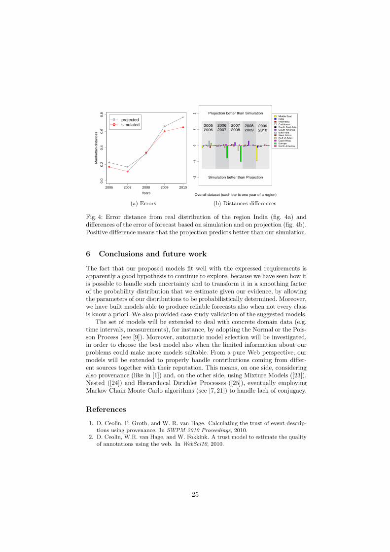
Fig. 4: Error distance from real distribution of the region India (fig. 4a) anddifferences of the error of forecast based on simulation and on projection (fig. 4b).Positive difference means that the projection predicts better than our simulation.

6 Conclusions and future work

The fact that our proposed models fit well with the expressed requirements isapparently a good hypothesis to continue to explore, because we have seen how itis possible to handle such uncertainty and to transform it in a smoothing factorof the probability distribution that we estimate given our evidence, by allowingthe parameters of our distributions to be probabilistically determined. Moreover,we have built models able to produce reliable forecasts also when not every classis know a priori. We also provided case study validation of the suggested models.

The set of models will be extended to deal with concrete domain data (e.g.time intervals, measurements), for instance, by adopting the Normal or the Pois-son Process (see [9]). Moreover, automatic model selection will be investigated,in order to choose the best model also when the limited information about ourproblems could make more models suitable. From a pure Web perspective, ourmodels will be extended to properly handle contributions coming from differ-ent sources together with their reputation. This means, on one side, consideringalso provenance (like in [1]) and, on the other side, using Mixture Models ([23]),Nested ([24]) and Hierarchical Dirichlet Processes ([25]), eventually employingMarkov Chain Monte Carlo algorithms (see [7, 21]) to handle lack of conjugacy.

References1. D. Ceolin, P. Groth, and W. R. van Hage. Calculating the trust of event descrip-

tions using provenance. In SWPM 2010 Proceedings, 2010.2. D. Ceolin, W.R. van Hage, and W. Fokkink. A trust model to estimate the quality

of annotations using the web. In WebSci10, 2010.

25

3. M. Davy and J. Tourneret. Generative supervised classification using dirichletprocess priors. IEEE Trans. Pattern Anal. Mach. Intell., 32:1781–1794, 2010.

4. P. Dirac. Principles of quantum mechanics. Oxford at the Clarendon Press, 1958.5. Andersen E. Sufficiency and exponential families for discrete sample spaces. Jour-

nal of the American Statistical Association, 65:1248–1255, 9 1970.6. C. Elkan. Clustering documents with an exponential-family approximation of the

Dirichlet compound multinomial distribution. In ICML, volume 148, pages 289–296. ACM, 2006.

7. M. D. Escobar and M. West. Bayesian density estimation and inference usingmixtures. Journal of the American Statistical Association, 90:577–588, 1994.

8. T. S. Ferguson. A Bayesian Analysis of Some Nonparametric Problems. The Annalsof Statistics, 1(2):209–230, 1973.

9. D. Fink. A Compendium of Conjugate Priors. Technical report, Cornell University,1995.

10. A. Fokoue, M. Srivatsa, and R. Young. Assessing trust in uncertain information.In ISWC, pages 209–224, 2010.

11. A. Gelman, J. B. Carlin, H. S. Stern, and D. B. Rubin. Bayesian Data Analysis.CRC Press, 2003.

12. R. Schlaifer H. Raiffa. Applied statistical decision theory. M.I.T. Press, 1968.13. M. Hazewinkel. Encyclopaedia of Mathematics, chapter De Finetti theorem.

Springer, 2001.14. B. He, M. Patel, Z. Zhang, and K. C. Chang. Accessing the deep web. Commun.

ACM, 50:94–101, May 2007.15. J. Hilgevoord and J. Uffink. Uncertainty in prediction and in inference. Foundations

of Physics, 21:323–341, 1991.16. E. F. Krause. Taxicab Geometry. Dover, 1987.17. P. Kvam and D. Day. The multivariate polya distribution in combat modeling.

Naval Research Logistics (NRL), 48(1):1–17, 2001.18. R. E. Madsen, D. Kauchak, and C. Elkan. Modeling word burstiness using the

Dirichlet distribution. In ICML, ICML ’05, pages 545–552. ACM, 2005.19. T. Minka. Estimating a Dirichlet distribution. Technical report, Microsoft Re-

search, 2003.20. P. Müller N. L. Hjort, C. Holmes and S. G. Walker. Bayesian Nonparametrics.

Cambridge University Press, 2010.21. R. M. Neal. Markov chain sampling methods for Dirichlet process mixture models.

Journal of Computational and graphical statistics, 9(2):249–265, 2000.22. J. Pitman. Exchangeable and partially exchangeable random partitions. Probab.

Theory Related Fields, 102(2):145–158, 1995.23. Carl Edward Rasmussen. The infinite gaussian mixture model. In In Advances in

Neural Information Processing Systems 12, pages 554–560. MIT Press, 2000.24. A. Rodriguez, D. B. Dunson, and A. E. Gelfand. The nested dirichlet process.

Journal of the American Statistical Assoc., 103(483):1131–1144, September 2008.25. Y. W. Teh, M. I. Jordan, M. J. Beal, and D. M. Blei. Hierarchical Dirichlet

processes. Journal of the American Statistical Assoc., 101(476):1566–1581, 2006.26. W3C. OWL Reference, August 2011. http://www.w3.org/TR/owl-ref/.27. W3C. Resource Definition Framework, August 2011. http://www.w3.org/RDF/.28. W3C. SPARQL, August 2011. http://www.w3.org/TR/rdf-sparql-query/.29. F. Wilcoxon. Individual Comparisons by Ranking Methods. Biometrics Bulletin,

1(6):80–83, 1945.30. E. Xing. Bayesian Haplotype Inference via the Dirichlet Process. In ICML, pages

879–886. ACM Press, 2004.

26

An Evidential Approach for Modeling and Reasoning on Uncertainty in Semantic Applications

Amandine Bellenger1,2, Sylvain Gatepaille1, Habib Abdulrab2, Jean-Philippe Kotowicz2

1 Cassidian – An EADS Company

Parc d'Affaires des Portes, 27106 Val-de-Reuil, France Amandine.Bellenger, Sylvain.Gatepaille@eads.com

2 LITIS Laboratory INSA de Rouen, Avenue de l’Université, 76801 Saint-Etienne-du-Rouvray, France

Habib.Abdulrab, Jean-Philippe.Kotowicz@insa-rouen.fr

Abstract. Standard semantic technologies propose powerful means for knowledge representation as well as enhanced reasoning capabilities to modern applications. However, the question of dealing with uncertainty, which is ubiquitous and inherent to real world domain, is still considered as a major deficiency. We need to adapt those technologies to the context of uncertain representation of the world. Here, this issue is examined through the evidential theory, in order to model and reason about uncertainty in the assertional knowledge of the ontology. The evidential theory, also known as the Dempster-Shafer theory, is an extension of probabilities and proposes to assign masses on specific sets of hypotheses. Further on, thanks to the semantics (hierarchical structure, constraint axioms and properties defined in the ontology) associated to hypotheses, a consistent frame of this theory is automatically created to apply the classical combinations of information and decision process offered by this mathematical theory.

Keywords: Ontologies, OWL, Uncertainty, Dempster-Shafer Theory, Belief Functions, Semantic Similarity.

1 Introduction

Uncertainty is an important characteristic of data and information handled by real-world applications. The term "uncertainty" refers to a variety of forms of imperfect knowledge, such as incompleteness, vagueness, randomness, inconsistency and ambiguity. In this approach, we consider only the epistemic uncertainty, due to lack of knowledge (incompleteness) and the inconsistency, due to conflicting testimonies or reports. This paper presents a proposal on a possible way to tackle the issue of representing and reasoning on this type of uncertainty in semantic applications, by using the Dempster–Shafer theory [1], also known as “evidential theory” or “belief function theory”. The general objective of our applications is to form the most informative and consistent view of the situation, observed by multiple sources. These observations populate our domain ontology. Thus, we consider that the uncertainty

27

has to be embodied in the instantiation rather than in the structural knowledge of ontology. One of our requirements is that a source can assign a belief on any instance without worrying of any level of granularity or disjointness of these instances. For example, one source could assign a belief on an instance of class Vehicle and, at the same time, another belief on an instance of type Car, which inherits from the class Vehicle.

The following section of this paper introduces the basic definitions and notations of the Dempster–Shafer theory. Section 3 presents our ontology modeling of the representation of uncertainty, using evidential theory. In the fourth section, we address how to reason with the evidential theory while benefiting from the semantics included in the domain ontology. Section 5 proposes to position our approach by comparing it with already existing works in the domain of uncertainty and the Semantic Web.

2 Basis of Dempster-Shafer Theory

The Dempster–Shafer theory [1] allows the combination of distinct evidence from different sources in order to calculate a global amount of belief for a given hypothesis. It is often presented as a generalization of the probability theory. It permits to manage uncertainties as well as inaccuracies and ignorance.

2.1 Frame of Discernment

Let Ω be the universal set, also called the discernment frame. It is the set of all the N states (hypothesis) under consideration: NHHH ,.., 21=Ω .

The universal set is supposed to be exhaustive and all hypotheses are exclusives. Exhaustivity refers to the closed-world principle. From this universal set, we can define a set, noted 2Ω. It is called the power set and is the set of all possible sub-sets of Ω, including the empty set. It is defined as follows:

Ω=Ω⊆=Ω ,...,,,,...,Ø,2 211 HHHHAA N .

2.2 Basic Mass Assignment and Belief Measures

A source, who believes that one or more states in the power set of Ω might be true, can assign belief mass to these states. Formally, a mass function is defined by:

[ ]1,02: →Ωm . (1)

It is also called a basic belief assignment and it has two properties:

0)Ø( =m and 1)(2

=∑Ω∈A

Am . (2)

This quantity differs from a probability since the total mass can be given either to singleton hypothesis Hn or to composite ones.

28

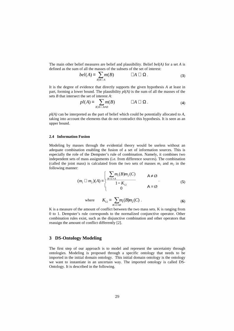
The main other belief measures are belief and plausibility. Belief bel(A) for a set A is defined as the sum of all the masses of the subsets of the set of interest:

∑⊆

=ABB

BmAbel )()( Ω⊆∀A . (3)

It is the degree of evidence that directly supports the given hypothesis A at least in part, forming a lower bound. The plausibility pl(A) is the sum of all the masses of the sets B that intersect the set of interest A:

∑≠∩

=Ø

)()(ABB

BmApl Ω⊆∀A . (4)

pl(A) can be interpreted as the part of belief which could be potentially allocated to A, taking into account the elements that do not contradict this hypothesis. It is seen as an upper bound.

2.4 Information Fusion

Modeling by masses through the evidential theory would be useless without an adequate combination enabling the fusion of a set of information sources. This is especially the role of the Dempster’s rule of combination. Namely, it combines two independent sets of mass assignments (i.e. from difference sources). The combination (called the joint mass) is calculated from the two sets of masses m1 and m2 in the following manner:

−=⊕∑

=∩

01

)()(

))((12

21

21 K

CmBm

AmmACB

A ≠ Ø

A = Ø

.

(5)

where )()( 2Ø

112 CmBmKCB∑

=∩

= . (6)

K is a measure of the amount of conflict between the two mass sets. K is ranging from 0 to 1. Dempster’s rule corresponds to the normalized conjunctive operator. Other combination rules exist, such as the disjunctive combination and other operators that reassign the amount of conflict differently [2].

3 DS-Ontology Modeling

The first step of our approach is to model and represent the uncertainty through ontologies. Modeling is proposed through a specific ontology that needs to be imported in the initial domain ontology. This initial domain ontology is the ontology we want to instantiate in an uncertain way. The imported ontology is called DS-Ontology. It is described in the following.

29

3.1 Structural Knowledge of the DS-Ontology

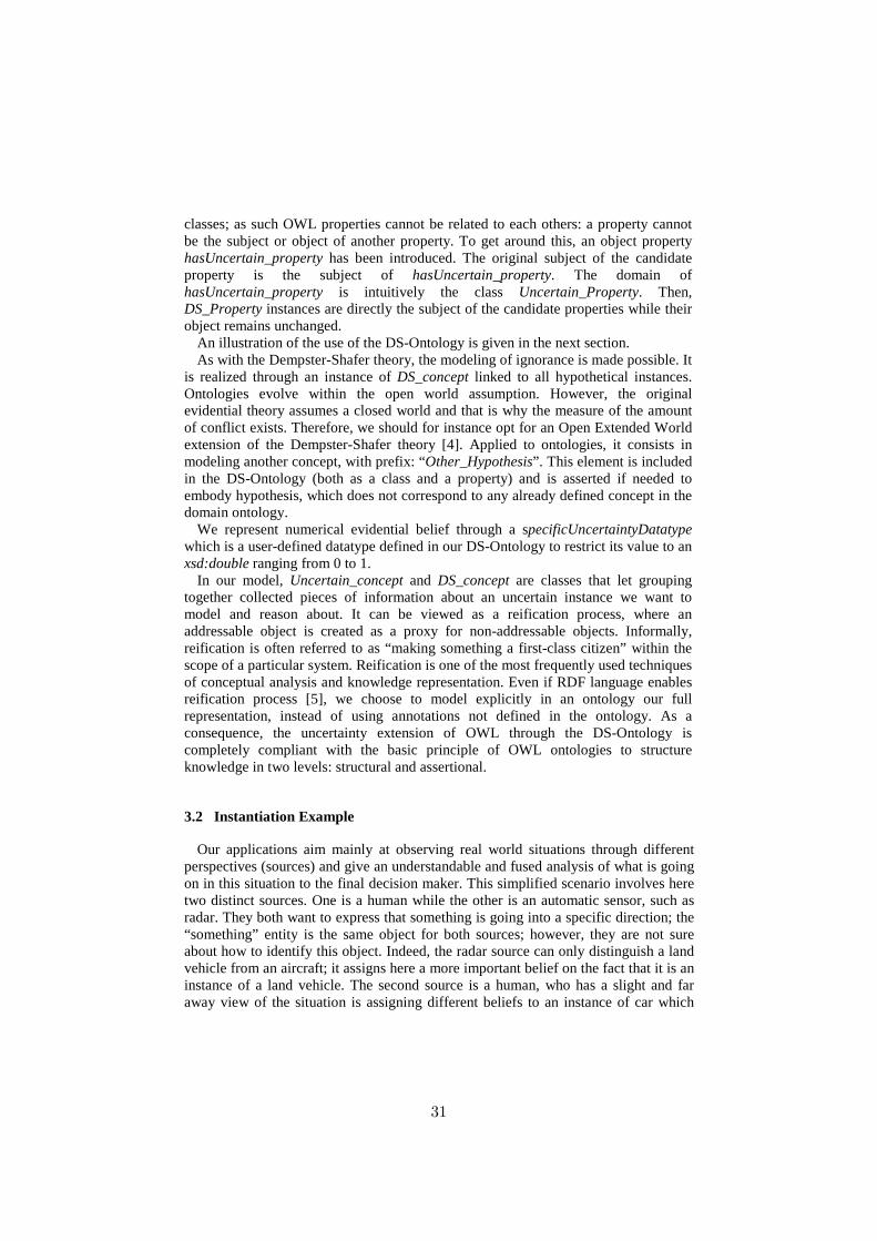
This ontology is a formal representation of the theory of Dempster-Shafer, as it proposes a shared understanding of the main concepts: mass, belief, plausibility, source, etc. It is non-domain specific, since one can use it in every area of knowledge. It has been coded in OWL2 language [3]. Hereafter is an informal schema of the terminology of DS-Ontology.

Fig. 1. Informal ontology structure schema. Yellow boxes represent OWL classes. Grey ones refer to datatypes (XML ones and user defined datatype). Arrows symbolize properties. Resources appearing without namespace prefix come from the DS-Ontology whose namespace is http://DS-Ontology.owl.

The main classes are Uncertain_concept and DS_concept. The DS_concept class links the hypothesis, with the source and the numerical amount of belief related to the hypothesis. The hypothesis consists either of a singleton or a union of hypotheses. Hypotheses are in fact instances of the domain ontology. Instances are either individuals of classes or instances of properties. The Uncertain_concept class links together all the DS_concept that are related to the same context. Indeed, the uncertainty is embodied by several candidate instances (with an assigned belief) and the uncertainty is concretely instantiated through one instance of Uncertain_concept. Uncertain_concept enables to retrieve the set of hypotheses under consideration, i.e. the power set 2Ω.

In order to represent uncertainty both on individuals and on asserted properties, DS_concept and Uncertain_concept have been specialized. They are specified in subclasses XX_class and XX_property (XX prefix representing both DS and Uncertain). Uncertain_concept is now an equivalent class to the union of Uncertain_property and Uncertain_class, while the latter two are disjoint. Respectively, this holds for DS-concept and its subclasses.

The hasDS_hypothesis object property relates an instance of DS_class to a set of candidate individuals. Concerning candidate properties, things have been done differently. Indeed, OWL properties are not first-class citizens, contrary to OWL

30

classes; as such OWL properties cannot be related to each others: a property cannot be the subject or object of another property. To get around this, an object property hasUncertain_property has been introduced. The original subject of the candidate property is the subject of hasUncertain_property. The domain of hasUncertain_property is intuitively the class Uncertain_Property. Then, DS_Property instances are directly the subject of the candidate properties while their object remains unchanged.

An illustration of the use of the DS-Ontology is given in the next section. As with the Dempster-Shafer theory, the modeling of ignorance is made possible. It

is realized through an instance of DS_concept linked to all hypothetical instances. Ontologies evolve within the open world assumption. However, the original evidential theory assumes a closed world and that is why the measure of the amount of conflict exists. Therefore, we should for instance opt for an Open Extended World extension of the Dempster-Shafer theory [4]. Applied to ontologies, it consists in modeling another concept, with prefix: “Other_Hypothesis”. This element is included in the DS-Ontology (both as a class and a property) and is asserted if needed to embody hypothesis, which does not correspond to any already defined concept in the domain ontology.

We represent numerical evidential belief through a specificUncertaintyDatatype which is a user-defined datatype defined in our DS-Ontology to restrict its value to an xsd:double ranging from 0 to 1.

In our model, Uncertain_concept and DS_concept are classes that let grouping together collected pieces of information about an uncertain instance we want to model and reason about. It can be viewed as a reification process, where an addressable object is created as a proxy for non-addressable objects. Informally, reification is often referred to as “making something a first-class citizen” within the scope of a particular system. Reification is one of the most frequently used techniques of conceptual analysis and knowledge representation. Even if RDF language enables reification process [5], we choose to model explicitly in an ontology our full representation, instead of using annotations not defined in the ontology. As a consequence, the uncertainty extension of OWL through the DS-Ontology is completely compliant with the basic principle of OWL ontologies to structure knowledge in two levels: structural and assertional.

3.2 Instantiation Example

Our applications aim mainly at observing real world situations through different perspectives (sources) and give an understandable and fused analysis of what is going on in this situation to the final decision maker. This simplified scenario involves here two distinct sources. One is a human while the other is an automatic sensor, such as radar. They both want to express that something is going into a specific direction; the “something” entity is the same object for both sources; however, they are not sure about how to identify this object. Indeed, the radar source can only distinguish a land vehicle from an aircraft; it assigns here a more important belief on the fact that it is an instance of a land vehicle. The second source is a human, who has a slight and far away view of the situation is assigning different beliefs to an instance of car which

31

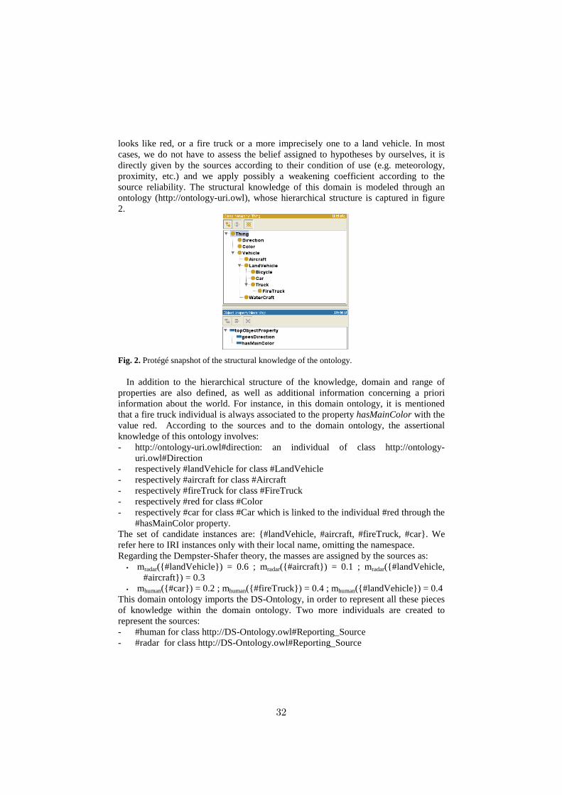
looks like red, or a fire truck or a more imprecisely one to a land vehicle. In most cases, we do not have to assess the belief assigned to hypotheses by ourselves, it is directly given by the sources according to their condition of use (e.g. meteorology, proximity, etc.) and we apply possibly a weakening coefficient according to the source reliability. The structural knowledge of this domain is modeled through an ontology (http://ontology-uri.owl), whose hierarchical structure is captured in figure 2.

Fig. 2. Protégé snapshot of the structural knowledge of the ontology.

In addition to the hierarchical structure of the knowledge, domain and range of properties are also defined, as well as additional information concerning a priori information about the world. For instance, in this domain ontology, it is mentioned that a fire truck individual is always associated to the property hasMainColor with the value red. According to the sources and to the domain ontology, the assertional knowledge of this ontology involves: - http://ontology-uri.owl#direction: an individual of class http://ontology-

uri.owl#Direction - respectively #landVehicle for class #LandVehicle - respectively #aircraft for class #Aircraft - respectively #fireTruck for class #FireTruck - respectively #red for class #Color - respectively #car for class #Car which is linked to the individual #red through the

#hasMainColor property. The set of candidate instances are: #landVehicle, #aircraft, #fireTruck, #car. We refer here to IRI instances only with their local name, omitting the namespace. Regarding the Dempster-Shafer theory, the masses are assigned by the sources as:

• mradar(#landVehicle) = 0.6 ; mradar(#aircraft) = 0.1 ; mradar(#landVehicle, #aircraft) = 0.3

• mhuman(#car) = 0.2 ; mhuman(#fireTruck) = 0.4 ; mhuman(#landVehicle) = 0.4 This domain ontology imports the DS-Ontology, in order to represent all these pieces of knowledge within the domain ontology. Two more individuals are created to represent the sources: - #human for class http://DS-Ontology.owl#Reporting_Source - #radar for class http://DS-Ontology.owl#Reporting_Source

32

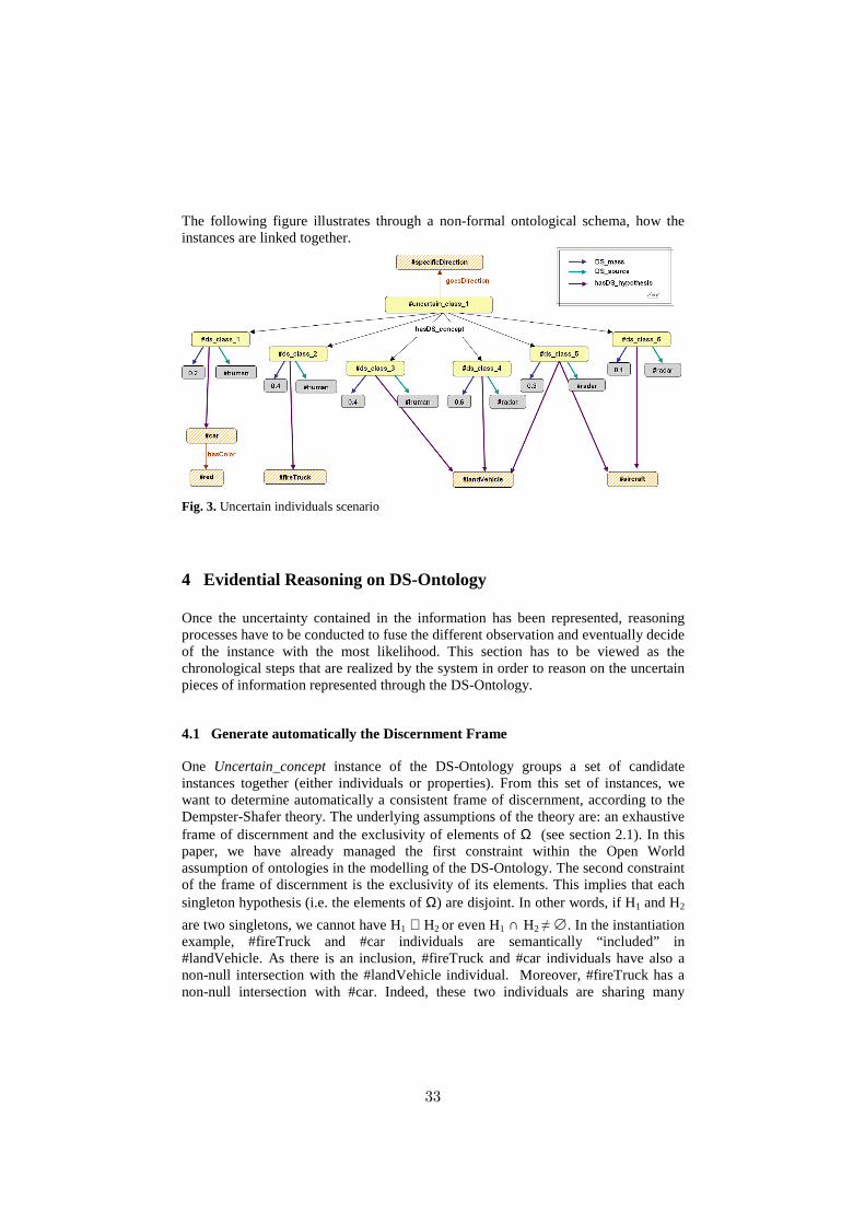
The following figure illustrates through a non-formal ontological schema, how the instances are linked together.

Fig. 3. Uncertain individuals scenario

4 Evidential Reasoning on DS-Ontology

Once the uncertainty contained in the information has been represented, reasoning processes have to be conducted to fuse the different observation and eventually decide of the instance with the most likelihood. This section has to be viewed as the chronological steps that are realized by the system in order to reason on the uncertain pieces of information represented through the DS-Ontology.

4.1 Generate automatically the Discernment Frame

One Uncertain_concept instance of the DS-Ontology groups a set of candidate instances together (either individuals or properties). From this set of instances, we want to determine automatically a consistent frame of discernment, according to the Dempster-Shafer theory. The underlying assumptions of the theory are: an exhaustive frame of discernment and the exclusivity of elements of Ω (see section 2.1). In this paper, we have already managed the first constraint within the Open World assumption of ontologies in the modelling of the DS-Ontology. The second constraint of the frame of discernment is the exclusivity of its elements. This implies that each singleton hypothesis (i.e. the elements of Ω) are disjoint. In other words, if H1 and H2

are two singletons, we cannot have H1 ⊂ H2 or even H1 ∩ H2 ≠ ∅. In the instantiation example, #fireTruck and #car individuals are semantically “included” in #landVehicle. As there is an inclusion, #fireTruck and #car individuals have also a non-null intersection with the #landVehicle individual. Moreover, #fireTruck has a non-null intersection with #car. Indeed, these two individuals are sharing many

33

characteristics in common: they are both land vehicles and their main colors are in both cases red.

To deal with this second constraint, we take into account the explicit and inferred semantics of the domain ontology to generate the discernment frame. The granularity of the set of candidate instances affects the generation of the discernment frame. The semantic will help us determining the inclusion of hypotheses as well as the semantic similarity between instances. The whole set of candidate instances will help us fixing a threshold for semantic distances.

4.1.1 Semantic Inclusion/Intersection The semantic inclusion is quite straightforward to determine. Indeed, in case the instances are property assertions, for example if a property P1 has for ancestor P2, then we say that P1 is included in P2. Otherwise, in case the instances are individuals and they have zero or the same properties (or some included property), then there is an inclusion. In all other cases, the inclusion does not hold.

Concerning semantic intersection, things go a little further. First of all, logically, if two instances have already a semantic inclusion, then they also have a non-null semantic intersection. In all other cases, we will consider that two instances have a non-null intersection when their semantic similarity is exceeding a certain threshold. More specifically, our similarity measure is a global function, which combines existing similarity measure defined in literature. As for individuals, it is a mixture of similarity measure of their respective types and similarity measures concerning their relations. Wu & Palmer similarity measure [6] is used to qualify the similarity between two instances based on their respective type. It takes into account the distance that separates two types in the hierarchy and their position with the root. Equation (7) depicts their formula. C1 and C2 are two classes. Class C is the immediate mother-class of C1 and C2 that subsumes both classes. depth(C) function is the number of edges separating C from the root. depthC(Ci) is the number of edges which separate Ci from the root while passing by C.

2)( + 1)(

)(*2)2,1(

CC CdepthCdepth

CdepthCCconSim = . (7)

The other combined similarity measures count the number of identical properties versus the number of different properties related to the two individuals. This is calculated both for object properties and datatype properties. On equation (8), I1 and I2 are the two individuals for which the global semantic similarity measure is calculated. For object properties (respectively for datatype properties), nbProp(I) is the number of object properties (resp. of datatype properties) of individual I. nbPropComm(I1,I2) is the number of common properties - identical predicate and related individual or value - for the two individuals I1 and I2. These three similarity measures focusing on the similarity of the types of individuals and their characteristics (through the datatype and object properties) are combined through a weighted mean.

)2( + )1(

)2,1(*2)2,1(

InbPropInbProp

IInbPropCommIIpropSim = . (8)

34

Once the cross-similarity measure of the set of all candidate instances is calculated, the threshold is fixed through a clustering method. The threshold is thus varying according to all the computed semantic similarities. This process permits to adapt the granularity of the set of candidate instances. It translates our general impression that the concept of a compact car is closer to the concept of minivan than of a plane’s; however the concept of a compact car is closer to the concept of plane than of a book’s. In the first case, the intersection should be brought by the pair (compact car, minivan), whereas in the latter, it should be brought by the pair of (compact car, plane). It should be noted that, in both cases, the concepts of compact car and plane have the same semantic similarity. As a consequence, the semantic intersection is seen as a Boolean condition on the similarity measure exceeding the threshold. Finally, we consider the evidential set inclusion (respectively intersection) as equivalent to the semantic inclusion (respectively intersection). In case of our scenario, the intersection and inclusion are graphically represented on the figure below.

Fig. 4. Inclusion and intersection of candidate instances

4.1.2 From the Set of Candidates Instances to the Discernment Frame Once the intersection and inclusion of candidate instances identified, we are able to set up a consistent frame of discernment. For this, we reframe the set of candidate instances into single or composite disjoint hypotheses. In case of a discovered intersection between two candidate instances #inst1 and #inst2, #inst1 is reformulated as the union of two singletons H1, Hinters and #inst2 as H 2, Hinters. In case of discovered inclusions between two candidate instances #inst1 and #inst2, where #inst1 is included in #inst2, #inst1 is represented by a single hypothesis H1 and #inst2 by the union of hypotheses H2, H1. Single hypotheses, grouped together, constitute the frame of discernment. In fact, each initial candidate instance belongs to the power-set of the frame of discernment. Taking our scenario, each candidate instance can now be decomposed as such: - #aircraft = H1 - #car = H2, H3 - #fireTruck = H3, H4 - #landVehicle = H2, H3, H4, H5 Indeed, relying on Figure 4, #aircraft instance has no intersection nor inclusion; thus, it constitutes a single hypothesis within the frame of discernment. The non-null intersection, between #fireTruck and #car instances, has been modeled through a common and shared single hypothesis: H3. Finally, the inclusion brought by #landVehicle results in the union of the set of single hypotheses of #fireTruck and #car, in addition to its own singleton H5.

35

4.2 Use Dempster-Shafer Calculations on DS-Ontology

Once the discernment frame has been obtained, we can reformulate in the Dempster-Shafer formalism, the basic mass assignment of the scenario: • mradar(H 2, H3, H4, H5) = 0.6 ; mradar(H 1) = 0.1 ; mradar(H 1, H2, H3, H4, H5) = 0.3 • mhuman(H 2, H3) = 0.2 ; mhuman(H 3, H4) = 0.4 ; mhuman(H 2, H3, H4, H5) = 0.4 We are now able to apply directly the classical combination rules found in the Dempster-Shafer theory, and then go through the decision process.

5 Related Work

During the last decade, approaches considering both uncertainty and the Semantic Web have been proposed. In this section, we mention some of them in order to position and compare our work. We consider their goal, underlying mathematical theory and processes.

Fuzzy and rough set theories aim to model vagueness and uncertainty. Regarding fuzzy sets, classes are considered to have unsharp definitions. fuzzyDL approach [7] aims to represent and reason about a membership function specifying the degree to which an instance belongs to a class. Even if it could be interesting to take into account fuzzy aspect of hypotheses especially those formulated by human sources, it is not the purpose of our approach to model more precisely our knowledge, but to decide among multi hypotheses and have a more coherent and reliable view of the situation. Approaches in [8, 9] are relying on rough set theory – which considers the indiscernability between objects. In that case, classes are not restricted to a crisp representation; they may be coarsely described with approximations. In [9], the author is using rough classes to generate new subclasses or relations by mining an important set of instances already existing. This can be part of the ontology engineering process. The goal is here also different to ours; however, some notions and process are similar. First, the design of a rough OWL ontology can be seen as the matching piece to our DS-Ontology for the Dempster-Shafer theory. Moreover, the use of p-indistinguishable properties notion for two individuals can be linked to our so-called common properties in Equation (8) when processing the similarity measure between two instances. Finally, descriptions for lower and upper approximation – through intersection and inclusion considerations - remind us the definition of the exclusivity of our frame of discernment; however, they consider here intersection and inclusion between two classes whereas we calculate it between two individuals.

Probabilistic adaptations or extensions (Pr-OWL [10], BayesOWL [11], Fire [12]) are more relevant to our objective of assessing the most likelihood instances that holds. However, probabilities suffer from the lack of ignorance and imprecision management in comparison to evidential theory.

Approaches in [13, 14 and 15] are more related to our chosen mathematical theory as they directly deal with evidential theory. [13] and [14] transform uncertain statements in belief networks. However, these network representations are themselves extensions of evidential theory. Moreover, they do not take into account the semantic attached to the hypotheses, in order to consider the most conflicting hypotheses or on

36

the inverse the implied hypotheses. Looking this way, they can be considered complementary to ours. A recent published approach [15] is concentrating on uncertain reasoning on instances of an ontology using the evidential theory and some similarity measures. While we handle the same mentioned tools, our process and aspiration are quite different. Indeed, their main objective is to propose an alternative ABox inductive reasoning - by classifying individuals (determining their class- or role- memberships or value for datatype properties) through a prediction based on an evidential nearest neighbor procedure. Their reasoning addresses here another way to tackle automatic inference from a classical ontology. This automatic inference aims to derive new or implicit knowledge about the current representation of the world, on the basis of the asserted knowledge. Whereas, our current reasoning goal is to rely on the semantic description of candidate instances (hypothesis) describing a same and unique entity or phenomenon in order to decide which candidate instances should be chosen.

Other reports enlarging the state-of-the-art to all ontology languages can be found in [17, 18].

6 Conclusion and Future Work

This paper proposes a solution in order to handle uncertainty within ontologies. Our approach is relying on current W3C standards. Modeling of uncertainty is realized through an imported pre-defined ontology: the DS-Ontology. Uncertain instantiation of the domain ontology is performed through the use of this imported DS-Ontology. The DS-Ontology relies on the theory of Dempster-Shafer, which manages uncertainty, as well as imprecision and ignorance. This paper has underlined some key issues that have to be dealt when implementing such parallelism between a formal mathematical theory to manage uncertainty and semantic world. The assumption of Open World in ontologies is one of these issues. Reasoning on uncertainty is made possible through an automatic generation of the frame of discernment. For that purpose, Boolean semantic operators, such as the intersection and inclusion, have been developed based on the semantic expressivity of the domain ontology. As a consequence, this paper provides a double and mutual contribution in the domains of the Semantic Web and of uncertain theories, which benefits clearly from the semantics of the hypotheses.

Further researches are also in discussion to extend the reasoning over the Boolean inclusion and intersection of candidate instances. Indeed, it could be interesting to keep the semantic similarity degree (which is a real ranging from 0 to 1) and use it instead of Boolean notions within the theory of Dempster-Shafer. This could be made by rearranging the basic measures of belief and plausibility and of the rules of combination.

37

References

1. Shafer, G.: A mathematical theory of evidence. Princeton University press Princeton, NJ, Volume 1 (1976)

2. Martin, A., Osswald, C., Dezert, J., Smarandache, F.: General combination rules for qualitative and quantitative beliefs, Journal of Advances in Information Fusion 3, 67-89, (2008)

3. Hitzler, P., Krötzsch, M., Parsia, B., Patel-Schneider, P.F., Rudolph, S.: OWL 2 Web Ontology Language Primer. W3C Recommendation 27 October 2009, World Wide Web Consortium (2009)

4. Royère, C., Gruyer, D., Cherfaoui, V.: Data association with believe theory, In Proceedings of the Third International Conference on Information Fusion, Paris, France (2000)

5. Manola, F., Miller, E., McBride, B.: RDF Primer W3C Recommendation (2004) 6. Wu, Z., Palmer, M.: Verb semantics and lexical selection. In Proceedings of the 32nd Annual

Meeting of the Associations for Computational Linguistics, pages 133–138, Las Cruces, New Mexico (1994)

7. Bobillo, F., Straccia, U.: FuzzyDL: An expressive fuzzy description logic reasoner, in IEEE International Conference on Fuzzy Systems 2008, pages 923–930. IEEE (2008)

8. Schlobach, S., Klein, M. C, Peelen, L.: Description Logics with Approximate Definitions: Precise Modeling of Vague Concepts. In Proceedings of the 20th International Joint Conference on Artificial Intelligence, IJCAI 07, Hyderabad, India (2007)

9. Keet, C.M.: Ontology engineering with rough concepts and instances. 17th International Conference on Knowledge Engineering and Knowledge Management (EKAW'10), P. Cimiano and H.S. Pinto (Eds.), Lisbon, Portugal, Springer LNAI 6317, 507-517 (2010)

10. Costa, P.C.G., Laskey, K.B.: PR-OWL: A framework for probabilistic ontologies, In Proceeding of the 2006 conference on Formal Ontology in Information Systems: Proceedings of the Fourth International Conference, pages 237–249, IOS Press (2006)

11. Ding, Z., Peng, Y., Pan, R.: BayesOWL: Uncertainty modeling in semantic web ontologies, Soft Computing in Ontologies and Semantic Web, pages 3–29 (2006)

12. Simou, N., Kollias, S.: Fire: A fuzzy reasoning engine for imprecise knowledge, In K-Space PhD Students Workshop, Berlin, Germany, volume 14, Citeseer (2007)

13. Essaid, A., Yaghlane, B.B.: BeliefOWL: An Evidential Representation in OWL Ontology, In International Semantic Web Conference, International Workshop on Uncertainty Reasoning for the Semantic Web, Washington DC, USA, page 77. Citeseer (2009)

14. Nikolov, A., Uren, V., Motta, E., de Roeck, A.: Using the Dempster-Shafer Theory of Evidence to Resolve ABox Inconsistencies, Uncertainty Reasoning for the Semantic Web I Lecture Notes in Computer Science, Volume 5327/2008, 143-160 (2008)

15. Fanizzi, N., d'Amato, C., Esposito, F.: Evidential Nearest-Neighbors Classification for Inductive ABox Reasoning. in Workshop on Uncertainty Reasoning for the Semantic Web URSW 2009, Washington D.C. - USA (2009)

16. Bellenger, A., Gatepaille, S.: Uncertainty in Ontologies: Dempster-Shafer Theory for Data Fusion Applications, in Workshop on the Theory of Belief Functions, Brest – France (2010)

17. Predoiu, L., Stuckenschmidt, H.: Probabilistic Models for the Semantic Web The Semantic Web for Knowledge and Data Management: Technologies and Practices (2009)

18. Lukasiewicz, T., Straccia, U.: Managing uncertainty and vagueness in description logics for the semantic web, Web Semantics: Science, Services and Agents on the World Wide Web, Elsevier, 6, 291-308 (2008)

38

Representing Sampling DistributionsIn P-SROIQ

Pavel Klinov1 and Bijan Parsia2

1 University of Arizona, AZ, USA pklinov@email.arizona.edu2 The University of Manchester, UK bparsia@cs.man.ac.uk

Abstract. We present a design for a (fragment of) Breast Cancer on-tology encoded in the probabilistic description logic P-SROIQ whichsupports determining the consistency of distinct statistical experimentalresults which may be described in diverse ways. The key contribution isa method for approximating sampling distributions such that the incon-sistency of the approximation implies the statistical inconsistency of thecontinuous distributions.

1 Introduction

The current amount of knowledge about breast cancer is overwhelming. Forexample, a meta-study conducted in 2006 by Key et al. [4] covered 98 uniquestudies focused only on the impact of a single risk factor, alcohol consumption. Atthe same time there are no common knowledge bases which would combine andformally represent findings produced by the multitude of studies.3 This makesit difficult to have a global view of breast cancer risk factors and, consequently,develop tools like risk assessment calculators.

The probabilistic description logic P-SROIQ can be used to represent gen-eral knowledge about breast cancer in the form of a probabilistic ontology (theBRC ontology) [5]. However, a general knowledge ontology need not support riskentailments for various combinations of risk factors — that is, compete (poorly)with narrowly specific risk calculators4 which have a direct implementation ofsimple equations derived from statistical risk models (such as the Gail model[2]). Instead, its main goal is to formally and unambiguously describe the back-ground theory of breast cancer embracing as many reliable findings as possibleand serving as a common knowledge base for more specific tools, such as riskassessment calculators or decision support systems. This sort of task seems tobe a better fit for a probabilistic logic.

The set of use cases for the general knowledge ontology is wider than for theBRC ontology. In addition to maintaining a birds-eye view of breast cancer, itmay be used for finding and analyzing inconsistencies in outcomes of different3 There are some lower level databases, such as ROCK (http://rock.icr.ac.uk/)—a

cancer specific functional genomic database. However, they do not explicitly repre-sent case study findings and do not support such services as risk assessment.

4 Such as http://www.cancer.gov/bcrisktool

39

studies. It can support studying mechanisms of interactions between risk factors,for example, how alcohol consumption affects estrogen level. Finally, it may playa useful role in planning and coordination of future medical studies by helping toidentify the most controversial or insufficiently studied risk factors or exposures.

In this paper, we present a design of general P-SROIQ ontology aboutbreast cancer (i.e., the BRC ontology) which incorporates a substantial amountof statistical knowledge. While we do not present a fully fleshed out instanceof this design, we do tackle a major representational challenge, namely, therepresentation of the statistical results of experiments. We present a method forapproximate representations of different sampling distributions and their use indetermining consistency between experimental data.

2 Preliminaries of P-SROIQP-SROIQ [8] is a probabilistic extension of the DL SROIQ [3]. It providesmeans for expressing probabilistic relationships between arbitrary SROIQ con-cepts and a certain class of probabilistic relationships between classes and indi-viduals. Any SROIQ, and thus OWL 2 DL (as it can be seen as a notationalvariant of SROIQ), ontology can be used as a basis for a P-SROIQ ontology,which facilitates transition from classical to probabilistic ontologies. We presumethe reader is reasonbly familiar with class/object oriented description logics suchas SROIQ, though very little in this paper turns on specific details.

The only syntactic construct in P-SROIQ (in addition to all of the SROIQsyntax) is the conditional constraint.

Definition 1 (Conditional Constraint). A conditional constraint is an ex-pression of the form (D|C)[l, u], where C and D are concept expressions inSRIQ (i.e., SROIQ without nominals) called evidence and conclusion, re-spectively, and [l, u] ⊆ [0, 1] is a closed real-valued interval. In the case where Cis > the constraint is called unconditional.

Ontologies in P-SROIQ are separated into a classical and a probabilisticpart. It is assumed that the set of individual names NI is partitioned onto twosets: classical individuals NCI and probabilistic individuals NPI .

Definition 2 (PTBox, PABox, and Probabilistic Knowledge Base). Aprobabilistic TBox (PTBox) is a pair PT = (T ,P) where T is a classical(finite) SROIQ TBox and P is a finite set of conditional constraints. A proba-bilistic ABox (PABox) is a finite set of conditional constraints associated witha probabilistic individual op ∈ NPI . A probabilistic knowledge base (or aprobabilistic ontology) is a triple PO = (T ,P, Popop∈NPI ), where the first twocomponents define a PTBox and the last is a a set of PABoxes.

Informally, a PTBox constraint (D|C)[l, u] expresses a conditional statementof the form “if a randomly chosen individual is an instance of C, the probabilityof it being an instance of D is in [l, u]”. A PABox constraint, which we write

40

as (D|C)o[l, u] where o is a probabilistic individual, states that “if a specificindividual (that is, o) is an instance of C, the probability of it being an instanceof D is in [l, u]”. For more details we refer the reader to [8].

3 The Classical Part

The classical part of a P-SROIQ ontology (or OWL part) provides a medicalvocabulary which can be used on its own in a variety of applications or used in therepresentation of probabilistic knowledge. In this paper we focus on providingan OWL terminology for probabilistic statements. The ontology contains thefollowing main class hierarchies (taxonomies):

Taxonomy of breast cancers Breast cancer is a heterogeneous disease. Somerisk factors can be associated with increase in risk of developing one partic-ular type of breast cancer and not the other. Thus it is important to classifytypes of breast cancer. In particular, our ontology distinguishes breast can-cers by hormone receptor status. Estrogen and progesterone positive breastcancers are modeled using concepts ERPositiveBRC and PRPositiveBRCwhile their complements are modeled using ERNegativeBRC andPRNegativeBRC (we use shorthands ER+/- and PR+/- with obvious mean-ing.). Another important classification is based on histology. The ontologydistinguishes between invasive and non-invasive (e.g. in situ) cancers.

Taxonomy of risk factors Dozens of risk factors are known so far. Some areestablished and strongly associate with increased risks, such as BRCA1(2)gene mutations, while others are controversial. The ontology should providevocabulary for both to support current and future findings. It includes ataxonomy of concepts rooted at RiskFactor. We distinguish between knownrisk factors (those which can be reported via a questionnaire, such as alcoholintake) and inferred risk factors which require medical examination.

Taxonomy of risks The ontology differentiates absolute and relative risks ofdeveloping breast cancer. Absolute risks are further divided into the life-time risk and the short-term risk. Relative risks are divided into increasedand reduced risks. Level of increases is a continuous variable which requiresdiscretization (see below).

The last two taxonomies induce the corresponding classifications of women,i.e., classes of women w.r.t. risk factors and w.r.t. risk. For example, any riskfactors RF gives rise to a class of women Woman u ∃hasRiskFactor.RF. Womenhaving various combinations of risk factors are modeled as conjunctive conceptexpressions. Analogously, given a certain kind of risk R the expression Woman u∃hasRisk.R models those women who are in the risk group R, for example, havemoderately increased risk of developing ER+ breast cancer. These taxonomiesof women may or may not be explicitly present in the ontology. In other words,it is possible, but not essential, to generate a concept name for each interestingclass of women since P-SROIQ (and our reasoner Pronto) allows for complexconcept expressions in conditional constraints.

41

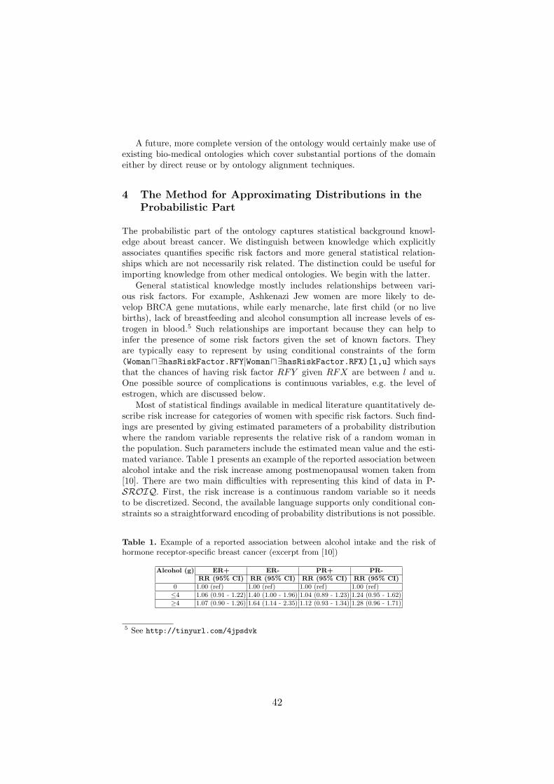
A future, more complete version of the ontology would certainly make use ofexisting bio-medical ontologies which cover substantial portions of the domaineither by direct reuse or by ontology alignment techniques.

4 The Method for Approximating Distributions in theProbabilistic Part

The probabilistic part of the ontology captures statistical background knowl-edge about breast cancer. We distinguish between knowledge which explicitlyassociates quantifies specific risk factors and more general statistical relation-ships which are not necessarily risk related. The distinction could be useful forimporting knowledge from other medical ontologies. We begin with the latter.

General statistical knowledge mostly includes relationships between vari-ous risk factors. For example, Ashkenazi Jew women are more likely to de-velop BRCA gene mutations, while early menarche, late first child (or no livebirths), lack of breastfeeding and alcohol consumption all increase levels of es-trogen in blood.5 Such relationships are important because they can help toinfer the presence of some risk factors given the set of known factors. Theyare typically easy to represent by using conditional constraints of the form(Womanu∃hasRiskFactor.RFY|Womanu∃hasRiskFactor.RFX)[l,u] which saysthat the chances of having risk factor RFY given RFX are between l and u.One possible source of complications is continuous variables, e.g. the level ofestrogen, which are discussed below.

Most of statistical findings available in medical literature quantitatively de-scribe risk increase for categories of women with specific risk factors. Such find-ings are presented by giving estimated parameters of a probability distributionwhere the random variable represents the relative risk of a random woman inthe population. Such parameters include the estimated mean value and the esti-mated variance. Table 1 presents an example of the reported association betweenalcohol intake and the risk increase among postmenopausal women taken from[10]. There are two main difficulties with representing this kind of data in P-SROIQ. First, the risk increase is a continuous random variable so it needsto be discretized. Second, the available language supports only conditional con-straints so a straightforward encoding of probability distributions is not possible.

Table 1. Example of a reported association between alcohol intake and the risk ofhormone receptor-specific breast cancer (excerpt from [10])

Alcohol (g) ER+ ER- PR+ PR-RR (95% CI) RR (95% CI) RR (95% CI) RR (95% CI)

0 1.00 (ref) 1.00 (ref) 1.00 (ref) 1.00 (ref)

≤4 1.06 (0.91 - 1.22) 1.40 (1.00 - 1.96) 1.04 (0.89 - 1.23) 1.24 (0.95 - 1.62)

≥4 1.07 (0.90 - 1.26) 1.64 (1.14 - 2.35) 1.12 (0.93 - 1.34) 1.28 (0.96 - 1.71)

5 See http://tinyurl.com/4jpsdvk

42

Discretization of a continuous variable is technically straightforward. We in-troduce a set of disjoint concept names each of which models women in thecorresponding group of risk. Specifically, we define concepts WomenAtWeakRisk,WomenAtModerateRisk and WomenAtHighRisk with the obvious meanings de-scribed using OWL 2 datatype support to describe the exact boundaries. Wehave chosen ranges (1, 1.5], (1.5, 3.0] and (3.0, + inf) respectively.6

The inability to represent distributions is a more severe limitation. It leavesthe modeler with the only option of approximating the continuous distributionusing a finite set of points. In other words, each distribution, for example, risk in-crease for women consuming a certain amount of alcohol, can be approximated byspecifying the probability that a randomly taken woman with the given exposurebelongs to a specific group of risk, i.e. WomenAtWeakRisk, WomenAtModerateRiskor WomenAtHighRisk. This is the semantics of P-SROIQ conditional constraints.

Assuming that the random variable is real-valued, a standard way of ap-proximating a continuous distribution is to take each interval and compute theprobability that the variable takes on a value in that interval. Then the ap-proximation of a distribution Pr(x) w.r.t. a finite set of intervals U is simply afunction P r such that P r(Ui) =

∫Ui

Pr(x)dx.

Unfortunately, this approximation of results of statistical experiments is un-satisfactory because it maps every interval to a single point. The problem is thatany arbitrarily small difference between two or more sampling distributions willresults in conflicting probabilistic statements for every interval (because thepoint-valued probabilities will be different) even though the results can confirmeach other from a purely statistical point of view. Consequently this approachdoes not support working with results reported by multiple studies.

Our goal is to approximate sampling distributions in P-SROIQ in a sta-tistically coherent way. Informally it means that satisfiability of probabilisticformulas representing two or more sampling distributions must agree with theirmutual statistical consistency, i.e., whether they support a common statisticalhypothesis. The hypothesis, in this case, is that there exists a distribution (notnecessarily a unique one) over G with parameters µ, σ such that it is supportedby all sampling distributions with the required level of confidence.

We assume a (finite) population G of size NG and a random variable Xwhich is normally distributed across G. We also make the realistic assumptionthat G is large enough so that evaluating X for all members of G is not feasible.A common approach is to take one or more random samples from G, evaluateX for them and estimate the actual distribution over G based on the samplingdistributions. We use µ, σ to denote the mean and the variance of the actualdistribution and X(i), S(i) for the mean and the variance of the sample X(i). Forsimplicity we finally assume that the population distribution is normal.

The mainstream approach for comparing two or more sampling distributionsis based on statistical hypothesis tests. For example, given two normal distribu-

6 The choice of intervals is obviously ambiguous but this issue is orthogonal to theapproximation method presented in this paper.

43

tions X(1), S(1), X(2), S(1) it is common to take X(1)−X(2), which is a normallydistributed random variable, and perform a z-test (or a Student’s t-test depend-ing on the sample sizes) to see if the difference can be taken as 0 with the requiredlevel of confidence. It amounts to calculating standard errors of the mean (SE)for both distributions and then computing the difference in units of SE. If theprobability of observing such difference given the null hypothesis,7 which can befound in standard tables, is low enough, e.g., ≤ 0.05, a statistician would acceptthe hypothesis that both distributions are consistent.

Our approach is slightly different from the outlined above. It is not based ontests but on confidence regions for sampling distributions. The approach, whichgeneralizes confidence intervals and dates back to Mood [9], is to estimate aregion Rγ in the parameter space for (µ, σ2) such that it will contain the µ, σ2

pair of the actual distribution 100(1 − γ)% times as the number of estimationsgoes to infinity. More formally, a 100(1− γ)% confidence region Rγ is a randomset for parameters (µ, σ2) based on a group of independent normally distributedvariables X (i.e., a sample) such that [1]:8

P ((µ, σ2) ∈ Rγ) = 1− γ, for all (µ, σ2) (1)

Informally, the confidence region specifies how far sampling distributions candeviate from the population distribution while supporting it with 100(1 − γ)%confidence. Following Mood [9] we will show that for the normal distribution theregion is a convex set and, therefore can be represented by boundary values of(µ, σ2) such that any sampling distribution inside the boundary will be consistentwith the current distribution.

Consider the sample X1, . . . , Xn where all Xi are independent random vari-ables with the normal distribution (N(µ, σ2)). Then X = 1

n

∑ni=1Xi and S2 =

1n−1

∑ni=1 (Xi −X)2, i.e., the sample mean and the sample variance, are ran-

dom variables. It is well known that X has the normal distribution N(µ, σ2

n ) (or,

equivalently, X−µσ/√n∼ N(0, 1)) while (n−1)S2/σ2 has the chi-square distribution

with n− 1 degrees of freedom [9].The standard tables for N(0, 1) and χ2

n−1 provide numbers a, b, c such thatfor fixed p1, p2 the following equalities hold [1]:

P (−a < X − µσ/√n< a) = p1,

P (b < (n− 1)S2/σ2 < c) = p2

7 The null hypothesis is a default position which, in this case, could be that thepopulation mean is different from at least one of X(1), X(2).

8 We deliberately leave out a precise definition of random set. For the purposes of thispaper it is sufficient to think of a random set as of a random variable which takeson subsets of some space.

44

The crucial fact is that the two random variables are independent (see [9] fora proof) which implies that:

p1p2 =

P (−a < X − µσ/√n< a, b <

(n− 1)S2

σ2< c) =

P (X − a σ√n< µ < X + a

σ√n,

(n− 1)S2

c< σ2 <

(n− 1)S2

b)

Thus, the 100(p1)(p2)% confidence region for (µ, σ2) takes the following form:

Rp1,p2(X,S) =

(µ, σ2) : X − α σ√n< µ < X + α

σ√n, (2)

(n− 1)S2

γ< σ2 <

(n− 1)S2

β

Figure 1 shows the joint confidence region R in the parameter space (µ, σ2).Note that it is possible, although technically messy, to generalize the definition(2) to the case of several independent sampling distributions. The simultane-ous confidence region for k samples X(1), . . . , X(k) will be a region in the 2k-dimensional parameter space which projections on each plane (µ(i), (σ(i))2) willlook as (2). Then the notion of consistency of sampling distributions can bedefined as follows (we limit the attention to two samples for clarity):

Fig. 1. Joint confidence region for (µ, σ2)

45

Definition 3. Let Pr(X(1)), P r(X(2)) be distributions on two samples X(1), X(2)

drawn independently from a population G. They are said to be consistent withconfidence 100p% if there exists a point (µ, σ2) which belongs to both Rp(X(1), S(1))and Rp(X(2), S(2)).

Now we can return to the issue of approximating a continuous samplingdistribution by a discrete set of points. Assume that the domain E of a continuousreal-valued random variable X is a disjoint union of a finite number of intervalsU = (−∞, r1], (r1, r2], . . . , (rl−1, rl], (rl,+∞). Then the approximation of thesampling distribution Pr(X) with mean and variance (X,S2) is the function P rwhich maps each interval Ui to the following real-valued set:

P r(Ui;X,S) = g(µ, σ2)|(µ, σ2) ∈ Rp1,p2(X,S) (3)

g(µ, σ2) =1√

2πσ2

∫

Ui

e−(x−µ)2

2σ2 dx

Now we are ready to define the notion of approximate consistency of samplingdistribution with respect to a set of intervals U :

Definition 4. Two sampling distributions Pr(X(1)), P r(X(2)) are approximatelyconsistent given a finite set of intervals U if P r(Ui;X(1), S(1)) ∩ P r(Ui;X(2), S(2))is non-empty for all Ui ∈ U .

As with any approximation, the utility of approximations of sampling distri-butions depends on what conclusions they help to draw about the distributionsthemselves. Given that we are interested in the matter of consistency, it is im-portant to understand the relationships between the notions of consistency andapproximate consistency of sampling distributions. Fortunately, consistency im-plies approximate consistency regardless of partitioning of the real line:

Theorem 1. If two sampling distributions Pr(X(1)), P r(X(2)) are consistent,then they are approximately consistent for any choice of real-valued intervals.

Proof. For the distribution Pr(X(1)) a confidence region Rp1,p2(X(1), S(1)) isconnected (see Definition 2). The function g(µ, σ2) (Definition 3) is continuous onit which implies that for any Ui, the set P r(Ui;X(1), S(1)) is a real-valued interval(l1, u1). Now consider a point µ0, σ

20 ∈ Rp1,p2(X(1), S(1)) ∩ Rp1,p2(X(2), S(2))

which exists since the distributions are consistent. It follows that l1 < g(µ0, σ20) <

u1 (and analogously l2 < g(µ0, σ20) < u2 for P r(Ui;X(2), S(2))), so g(µ0, σ

20) is

a common point for both approximations on Ui. As such the distributions areapproximately consistent.

The following corollary from the above theorem is at heart of our method.As we demonstrate below, the inconsistency of approximations can be provedby logical reasoning in P-SROIQ (i.e., by solving the probabilistic satisfiabil-ity problem), which means that the result enables approximate reasoning about

46

sampling distributions in a purely logical way. Even though the power of such rea-soning is currently limited to consistency checking, its integration with OWL/DLreasoning and the ability to use common, formally defined terminology for rep-resentation of statistical experiments is promising.

Corollary 1. If sampling distributions Pr(X(1)), P r(X(2)) are approximatelyinconsistent for some choice of real-valued intervals, then they are inconsistent.

5 Example of Approximate Modelling

Now we present an example of approximate representation of sampling distri-butions in P-SROIQ. The task is to take two results of statistical experimentsaimed at investigating associations between alcohol consumption and the in-creased risk of breast cancer among postmenopausal women. Unfortunately it iscommon for medical papers to not explicitly present all parameters that char-acterize results of their statistical analyses. Typically, only the estimated meanand the confidence interval are presented while, for example, the kind of distri-bution is left to the reader to infer from other information. Due to that fact andbecause the approach above has only been developed for normal distributions,we illustrate it on an artificial example. The information given in the exampleis analogous to that given in medical literature, e.g. [10, 11], but is complete inthe sense that all parameters and the type of sampling distributions are known.

Example 1. Consider two hypothetical papers which report results of indepen-dent studies of associations between alcohol consumption among postmenopausalwomen and their relative risk of developing breast cancer. According to studyA the mean relative risk (RR) of ER+ breast cancer for women drinking ≥ 4gof ethanol a day is 1.8 and has variance of 0.5. Study B has reported that themean RR of ER+ breast cancer for the same level of drinking is 2.2 (variance0.7). The number of cases in the studies was 230 and 150 respectively.

We propose the following four step procedure for an approximate representa-tion of statistical results, similar to those in the example above, in P-SROIQ:

1. Preparing concepts The first step is to define the concepts/roles usedto describe the distribution. In our case evidence concepts should describe cat-egories of women with respect to specific risk factors, e.g. alcohol intake, whileconclusion concepts describe groups of women stratified by risk increase. For in-stance, the concept expression C ≡ Womanu ∃hasRiskFactor.(PostmenopauseuModerateConsumption) is used to model postmenopausal women with moderatelevel of alcohol intake.9 On the other hand the expression:

D ≡ Woman u ∃hasRisk.(ModeratelyIncreasedRisk u ∃riskOf.ERPositiveBRC)

9 The level of intake is a continuous variable which we also split onto categoriesLimitedConsumption, ModerateConsumption and HeavyConsumption which corre-spond to ≤ 4, 4− 9.9 and ≥ 10g of ethanol per day.

47

models women who are at moderately increased risk of developing ER-positivebreast cancer. Using these expressions the modeler can specify the probabilitythan a random women the class C also belong the risk group D as (D|C)[l,u].

2. Determining parameters of sampling distributions (if required)Sometimes parameters of sampling distributions can be determined from otherinformation. For example, knowing the kind of distribution, sample mean, samplesize, confidence interval and the methodology of its estimation, one can calculatethe sample variance.10 In our case it is not needed as the distributions are normaland the parameters are known.

3. Choosing intervals Choice of intervals for an approximation of a con-tinuous random variable is driven by balancing the quality of the approxima-tion (i.e., how closely it models the continuous distribution) and the number ofstatements required. The latter has a direct impact on performance. For Ex-ample 1 we use three concepts WomenAtWeakRisk, WomenAtModerateRisk andWomenAtHighRisk which correspond to relative risk intervals of (1,1.5], (1.5,3.0] and (3.0,+∞) respectively.

4. Computing the approximation The final (and the central) step is tocompute probability intervals for the statements that approximate the contin-uous distribution. Each statement specifies the lower and upper probabilitiesthat the continuous random variable X will fall into an interval Ui given thatparameters of the distribution can vary within the confidence region (2). Moreformally, given the interval Ui, e.g. (1,1.5] for WomenAtWeakRisk, and the sam-pling distribution (X,S2) the interval [li, ui] can be computed by solving thefollowing non-linear optimization problem ():

li (resp. ui) = min (resp. max) g(µ, σ2) s.t. (4)

(µ, σ2) ∈ Rp1,p2(X,S)

g(µ, σ2) =1√

2πσ2

∫

Ui

e−(x−µ)2

2σ2 dx

In other words, [li, ui]=[inf P r(Ui;X,S), sup P r(Ui;X,S)].The last preparatory step is to calculate confidence regions according to (2).

The 95% confidence regions for distributions (X(1), S(1)), (X(2), S(2)) in Example1 (abbreviated as R(1)

0.95 and R(2)0.95) are defined by the following inequalities:

R(1)0.95 =

(µ, σ2) : 1.8− 2.241σ√

230< µ < 1.8 +

2.241σ√230

, 0.409 < σ2 < 0.623

R(2)0.95 =

(µ, σ2) : 2.2− 2.241σ√

150< µ < 2.2 +

2.241σ√150

, 0.548 < σ2 < 0.923

10 The variable T = (X − µ)/(S/√n) has the t-dustribution with n − 1 degrees

of freedom. Confidence interval is standardly computed as [X − a,X + a] wherea = t 1−α

2 ,n−1S√n

(t 1−α2 ,n−1

is the α−percentile of the Student distribution). If the

confidence interval and α are known, then S can be calculated.

48

Now the optimization problem (4) can be solved numerically11 to obtain thefollowing approximations for both sampling distributions:

inf P r((1, 1.5];X(1), S(1)) = 0.219 sup P r((1, 1.5];X(1), S(1)) = 0.298

inf P r((1.5, 3.0];X(1), S(1)) = 0.655 sup P r((1.5, 3.0];X(1), S(1)) = 0.878

inf P r((3.0,+∞);X(1), S(1)) = 0.239 sup P r((3.0,+∞);X(1), S(1)) = 0.586

inf P r((1, 1.5];X(2), S(2)) = 0.116 sup P r((1, 1.5];X(2), S(2)) = 0.224

inf P r((1.5, 3.0];X(2), S(2)) = 0.562 sup P r((1.5, 3.0];X(2), S(2)) = 0.769

inf P r((3.0,+∞);X(2), S(2)) = 0.189 sup P r((3.0,+∞);X(2), S(2)) = 0.568

So, for this example, the sampling distributions are approximately representedin P-SROIQ using the following conditional constraints.

(W u ∃hR.(WeaklyIncreasedRisk u ∃riskOf.ERPositiveBRC)|C)[0.219, 0.298],

(W u ∃hR.(ModeratelyIncreasedRisk u ∃riskOf.ERPositiveBRC)|C)[0.655, 0.878],

(W u ∃hR.(StronglyIncreasedRisk u ∃riskOf.ERPositiveBRC)|C)[0.239, 0.586]and

(W u ∃hR.(WeaklyIncreasedRisk u ∃riskOf.ERPositiveBRC)|C)[0.116, 0.224],

(W u ∃hR.(ModeratelyIncreasedRisk u ∃riskOf.ERPositiveBRC)|C)[0.562, 0.769],

(W u ∃hR.(StronglyIncreasedRisk u ∃riskOf.ERPositiveBRC)|C)[0.189, 0.568]where W and hR abbreviate Woman and hasRisk, respectively and

C ≡ W u ∃hasRiskFactor.(Postmenopause u ModerateConsumption)

Probabilistic consistency of the above set of statements can be proved bysolving the probabilistic satisfiability problem (PSAT). Modern algorithms candecide PSAT for over a thousand of P-SROIQ statements (in addition to thou-sands of OWL axioms), so the method could be computationally practical [6].

6 Conclusion

Checking consistency of sampling distributions in P-SROIQ may well appearcumbersome and pointless given that the same task can be done in a muchsimpler way and without any logical reasoning, e.g. via testing or by analyzingconfidence regions. However, our aim is not to reduce statistical testing to log-ical reasoning (that aim is indeed pointless). Our aim is to represent results ofstatistical experiments using common, unambiguously defined logical vocabularyand be able to reason about them. Even though probabilistic reasoning aboutstatistical results is currently limited to approximate consistency checking, the11 We use Wolfram Mathematica for this purpose.

49

potential benefits are in combining it with reasoning about the classical knowl-edge. For example, the BCRA ontology contains a little taxonomy of breastcancers by hormone receptor status. This enables us to combine results of thestudies which are of different levels of granularity. For instance, Sellers et al. [10]report associations between alcohol intake and ER(+/-) breast cancer risk, whileSuzuki et al. [11] divide it further to ER(+/-)PR(+/-) risks. In that simple casenon-logical reasoning about the reported results becomes much less straightfor-ward, while studies can also distinguish histologic types of breast cancer (see [7]).In such complex situations reasoning about findings does involve reasoning aboutbackground knowledge, e.g. the taxonomy of breast cancers, so a combination ofOWL and probabilistic reasoning is potentially beneficial.

References

1. Arnold, B.C., Shavelle, R.M.: Joint confidence sets for the mean and variance of anormal distribution. The American Statistician 52(2), 133–140 (1998)

2. Gail, M.H., Brinton, L.A., Byar, D.P., Corle, D.K., Green, S.B., Schairer, C., Mul-vihill, J.J.: Projecting individualized probabilities of developing breast cancer forwhite females who are being examined annually. Journal of the National CancerInstitute 81(25), 1879–1886 (1989)

3. Horrocks, I., Kutz, O., Sattler, U.: The even more irresistible SROIQ. In: Knowl-edge Representation and Reasoning. pp. 57–67 (2006)

4. Key, J., Hodgson, S., Omar, R.Z., Jensen, T.K., Thompson, S.G., Boobis, A.R.,Davies, D.S., Elliott, P.: Meta-analysis of studies of alcohol and breast cancer withconsideration of the methodological issues. Cancer Causes Control 17, 759–770(2006)

5. Klinov, P., Parsia, B.: Probabilistic modeling and OWL: A user oriented intro-duction into P-SHIQ(D). In: OWL: Experiences and Directions (2008), http:

//www.webont.org/owled/2008/papers/owled2008eu_submission_32.pdf

6. Klinov, P., Parsia, B.: A hybrid method for probabilistic satisfiability. In: CADE.pp. 354–368 (2011)

7. Lew, J.Q., Freedman, N.D., Leitzmann, M.F., Brinton, L.A., Hoover, R.N., Hollen-beck, A.R., Schatzkin, A., Park, Y.: Alcohol and risk of breast cancer by histologictype and hormone receptor status in postmenopausal women the nih-aarp diet andhealth study. American Journal of Epidemiology 170(3), 308–317 (2009)

8. Lukasiewicz, T.: Expressive probabilistic description logics. Artificial Intelligence172(6-7), 852–883 (2008)

9. Mood, A.M.: Introduction to the Theory of Statistics. McGraw-Hill (1950)10. Sellers, T.A., Vierkant, R.A., Cerhan, J.R., Gapstur, S.M., Vachon, C.M., Olson,

J.E., Pankratz, V.S., Kushi, L.H.: Interaction of dietary folate intake, alcohol, andrisk of hormone receptor-defined breast cancer in a prospective study of post-menopausal women. Cancer Epidemiology, Biomarkers and Prevention 11, 1104–1107 (2002)

11. Suzuki, R., Ye, W., Rylander-Rudqvist, T., Saji, S., Colditz, G.A., Wolk, A.: Al-cohol and postmenopausal breast cancer risk defined by estrogen and progesteronereceptor status: A prospective cohort study. Journal of the National Cancer Insti-tute 97(21), 1601–1608 (2005)

50

Finite Lattices Do Not Make Reasoning InALCI Harder

Stefan Borgwardt and Rafael Penalozastefborg,penaloza@tcs.inf.tu-dresden.de

Theoretical Computer Science, TU Dresden, Germany

Abstract. We consider the fuzzy logic ALCI with semantics based on afinite residuated lattice. We show that the problems of satisfiability andsubsumption of concepts in this logic are ExpTime-complete w.r.t. gen-eral TBoxes and PSpace-complete w.r.t. acyclic TBoxes. This matchesthe known complexity bounds for reasoning in crisp ALCI.

1 Introduction

OWL 2, the current standard ontology language for the semantic web, is basedon the crisp description logic (DL) SROIQ(D). As a crisp logic, it is not wellsuited to express vague or imprecise concepts, such as HighTemperature, that canbe found in numerous domains; prominently, in the biomedical area.

Fuzzy extensions of DLs have been studied for over a decade, and the litera-ture on the topic is very extensive (see [15] for a survey). However, most of thoseapproaches are based on the very simple Zadeh semantics where conjunction isinterpreted as the minimum, with truth values ranging over the interval [0, 1]of rational numbers. The last lustrum has seen a shift towards more general se-mantics for treating vagueness. On the one hand, the use of continuous t-normsas the underlying interpretation function for conjunction was proposed in [14].On the other hand, [18] allows lattice-based truth values, but still restricts toZadeh-like semantics.

Most of the work since then has focused on t-norm-based semantics over theunit interval; yet, ontologies are usually restricted to be unfoldable or acyclic [4–6]. Indeed, very recently it has been shown that general concept inclusion axioms(GCIs) can cause undecidability even in fuzzy DLs based on ALC [2, 3, 9, 11].These results motivate restricting the logics, e.g. to finitely-valued semantics.

If one considers the Lukasiewicz t-norm over finitely many values, then rea-soning is decidable even for very expressive DLs, as shown in [7] through areduction to crisp reasoning. When restricted to ALC without terminologicalaxioms, concept satisfiability is PSpace-complete as in the crisp case [10].1 Inthe presence of general TBoxes, this problem becomes ExpTime-complete [8, 9],again matching the complexity of the crisp case, even if arbitrary (finite) latticesand t-norms are allowed. However, the complexity of subsumption of concepts

1 The paper [10] considers a syntactic variant of fuzzy ALC with only one role.

51

was left as an open problem, as the standard reduction used in crisp DLs doesnot work with general t-norm semantics.

In this paper, we improve these complexity results to the fuzzy logic ALCILover finite lattices with general and acyclic TBoxes. More precisely, we show thatin this logic, concept satisfiability is ExpTime-complete w.r.t. general TBoxes,and PSpace-complete w.r.t. acyclic TBoxes. Moreover, the same complexitybounds also hold for deciding subsumption between concepts.

2 Preliminaries

We will first give a short introduction to residuated lattices, which will be usedfor defining the semantics of our logic.2 Afterwards, we recall some results fromautomata theory that will allow us to obtain tight upper bounds for the com-plexity of deciding satisfiability and subsumption of concepts.

2.1 Residuated Lattices

A lattice is an algebraic structure (L,∨,∧) over a carrier set L with two binaryoperations join ∨ and meet ∧ that are idempotent, associative, and commutativeand satisfy the absorption laws `1 ∨ (`1 ∧ `2) = `1 = `1 ∧ (`1 ∨ `2) for all`1, `2 ∈ L. L induces the ordering `1 ≤ `2 iff `1 ∧ `2 = `1 for all `1, `2 ∈ L. Lis called distributive if ∨ and ∧ distribute over each other, finite if L is finite,and bounded if it has a minimum and a maximum element, denoted as 0 and 1,respectively. It is complete if joins and meets of arbitrary subsets T ⊆ L, denotedby

∨t∈T t and

∧t∈T t respectively, exist. Every finite lattice is also bounded and

complete. Whenever it is clear from the context, we will simply use the carrierset L to represent the lattice (L,∨,∧).

A De Morgan lattice is a bounded distributive lattice extended with an in-volutive and anti-monotonic unary operation ∼, called (De Morgan) negation,satisfying the De Morgan laws ∼(`1∨`2) = ∼ `1∧∼ `2 and ∼(`1∧`2) = ∼ `1∨∼ `2for all `1, `2 ∈ L.

A residuated lattice is a lattice L extended with two binary operators ⊗(called t-norm) and ⇒ (called residuum) such that ⊗ is associative, commuta-tive, and has 1 as its unit and for every `1, `2, `3 ∈ L, `1⊗`2 ≤ `3 iff `2 ≤ `1 ⇒ `3holds. In a complete residuated lattice L, `1 ⇒ `2 =

∨x | `1 ⊗ x ≤ `2.3 Asimple consequence of this is that for every `1, `2 ∈ L, (i) 1 ⇒ `1 = `1, and (ii)`2 ≤ `2 iff `1 ⇒ `2 = 1. Additionally, the t-norm ⊗ is always monotonic.

In a residuated De Morgan lattice L, one can define the t-conorm ⊕ as`1 ⊕ `2 := ∼(∼ `1 ⊗ ∼ `2). For example, the meet operator `1 ∧ `2 defines at-norm; its t-conorm is `1 ∨ `2.

2 For a more comprehensive view on residuated lattices, we refer the reader to [13, 12].3 We could also define the operator ⇒ using this supremum, even if the complete

lattice L is not residuated without affecting the results from Section 4.

52

In the following section, we will describe the fuzzy description logic ALCIL,whose semantics uses the residuum ⇒ and the negation ∼. We emphasize, how-ever, that the reasoning algorithm presented in Section 4 can be used with anychoice of operators, as long as these are computable. In particular this meansthat our algorithm could also deal with other variants of fuzzy semantics, e.g.so-called Zadeh semantics [8, 18].

2.2 PSpace Automata

To obtain upper bounds for the complexity of reasoning in ALCIL, we willmake a reduction to the emptiness problem of looping automata on infinitetrees. These automata receive as input the (unlabeled) infinite k-ary tree K∗ forK := 1, . . . , k with k ∈ N. The nodes of this tree are represented as wordsin K∗: the empty word ε represents the root node, and ui represents the i-thsuccessor of the node u. A path is a sequence v1, . . . , vm of nodes such that v1 = εand each vi+1 is a direct successor of vi.

Definition 1 (looping automaton). A looping automaton (LA) is a tupleA = (Q, I,∆) where Q is a finite set of states, I ⊆ Q a set of initial states,and ∆ ⊆ Q×Qk the transition relation. A run of A is a mapping r : K∗ → Qassigning states to each node of K∗ such that r(ε) ∈ I and for every u ∈ K∗ wehave (r(u), r(u1), . . . , r(uk)) ∈ ∆. The emptiness problem for LA is to decidewhether a given LA has a run.

The emptiness of LA can be decided in polynomial time using a bottom-upapproach [19]. Alternatively, one can use a top-down approach, which relies onthe fact that if there is a run, then there is also a periodic run. To speed up thetop-down search, one wants to find the period of a run as early as possible. Thismotivates the notion of blocking automata.

Definition 2 (m-blocking). Let A = (Q,∆, I) be a looping automaton. Wesay that A is m-blocking for m ∈ N if every path v1, . . . , vm of length m in arun r of A contains two nodes vi and vj (i < j) such that r(vj) = r(vi).

Clearly, every looping automaton is m-blocking for every m > |Q|. However,the main interest in blocking automata arises when one can find a smaller boundon m. One way to reduce this limit is through a so-called faithful family offunctions.

Definition 3 (faithful). Let A = (Q,∆, I) be a looping automaton on k-arytrees. The family of functions fq : Q → Q for q ∈ Q is faithful w.r.t. A if forall q, q0, q1, . . . , qk ∈ Q,

– if (q, q1, . . . , qk) ∈ ∆, then (q, fq(q1), . . . , fq(qk)) ∈ ∆, and– if (q0, q1, . . . , qk) ∈ ∆, then (fq(q0), fq(q1), . . . , fq(qk)) ∈ ∆.

The subautomaton AS = (Q,∆S , I) of A induced by this family has the transi-tion relation ∆S = (q, fq(q1), . . . , fq(qk)) | (q, q1, . . . , qk) ∈ ∆.

53

Lemma 4 ([1]). Let A be a looping automaton and AS its subautomaton in-duced by a faithful family of functions. A has a run iff AS has a run.

The construction that we will present in Section 4 produces automata thatare exponential on the size of the input. For such cases, it has been shown thatif the automata are m-blocking for some m bounded polynomially on the sizeof the input (that is, logarithmically on the size of the automaton), then theemptiness test requires only polynomial space.

Definition 5 (PSpace on-the-fly construction). Assume that we have aset I of inputs and a construction that yields, for every i ∈ I, an mi-blockingautomaton Ai = (Qi, ∆i, Ii) working on ki-ary trees. This construction is calleda PSpace on-the-fly construction if there is a polynomial P such that, for everyinput i of size n

– mi ≤ P (n) and ki ≤ P (n),– every element of Qi is of a size bounded by P (n), and– one can non-deterministically guess in time bounded by P (n) an element ofIi, and, for a state q ∈ Qi, a transition from ∆i with first component q.

Theorem 6 ([1]). If the looping automata Ai are obtained from the inputs i ∈ Iby a PSpace on-the-fly construction, then the emptiness problem for Ai can bedecided in PSpace.

In Section 5 we will use this theorem to give PSpace upper bounds on thecomplexity of reasoning in the logic ALCIL, which we introduce next.

3 The Fuzzy Logic ALCIL

For the rest of this paper, L denotes a fixed residuated, complete De Morganlattice with the t-norm ⊗. The fuzzy description logic ALCIL is a generalizationof the crisp DL ALCI that uses the elements of L as truth values, instead ofjust the Boolean true and false. The syntax of ALCIL is the same as in ALCI:given the sets NC and NR of concept and role names, the set of complex roles isNR ∪ r− | r ∈ NR, and ALCIL concepts are built using the syntactic rule

C ::= A | C1 u C2 | C1 t C2 | ¬C | ∃s.C | ∀s.C | > | ⊥,

where A ∈ NC and s is a complex role. For a complex role s, the inverse of s(denoted by s) is s− if s ∈ NR and r if s = r−.

The semantics of this logic is based on interpretation functions that mapevery concept C to a function specifying the membership degree of every domainelement to C.

Definition 7 (semantics of ALCIL). An interpretation is a pair I = (∆I , ·I)where ∆I is a non-empty (crisp) domain and ·I is a function that assigns toevery concept name A and every role name r functions AI : ∆I → L andrI : ∆I ×∆I → L, respectively. The function ·I is extended to ALCIL conceptsas follows for every x ∈ ∆I :

54

– >I(x) = 1, ⊥I(x) = 0,– (C uD)I(x) = CI(x)⊗DI(x), (C tD)I(x) = CI(x)⊕DI(x),– (¬C)I(x) = ∼CI(x),– (∃s.C)I(x) =

∨y∈∆I sI(x, y)⊗ CI(y),

– (∀s.C)I(x) =∧y∈∆I sI(x, y)⇒ CI(y),

where (r−)I(x, y) = rI(y, x) for all x, y ∈ ∆I and r ∈ NR.

Notice that, unlike in crisp ALCI, existential and universal quantifiers arenot dual to each other, i.e. in general, (¬∃s.C)I(x) = (∀s.¬C)I(x) does not hold.

The axioms of this logic also have an associated lattice value, which expressesthe degree to which the restriction must be satisfied.

Definition 8 (axioms). Terminological axioms are (labeled) concept defini-tions of the form 〈A .= C, `〉 or (labeled) general concept inclusions (GCIs)〈C v D, `〉, where A ∈ NC, C,D are ALCIL concepts, and ` ∈ L.

A general TBox is a finite set of GCIs. An acyclic TBox is a finite set ofconcept definitions such that every concept name occurs at most once in the left-hand side of an axiom, and there is no cyclic dependency between definitions. ATBox is either a general TBox or an acyclic TBox.4

An interpretation I satisfies the concept definition 〈A .= C, `〉 if for everyx ∈ ∆I , (AI(x) ⇒ CI(x)) ⊗ (CI(x) ⇒ AI(x)) ≥ ` holds. It satisfies the GCI〈C v D, `〉 if for every x ∈ ∆I , CI(x)⇒ DI(x) ≥ `. I is a model of the TBoxT if it satisfies all axioms in T .

If T is an acyclic TBox, then all concept names occuring on the left-handside of some axiom of T are called defined, all others are called primitive. If T isa general TBox, then all concept names appearing in it are primitive. A conceptis an atom if it is either a primitive concept name, or it is a quantified concept,i.e. a concept of the form ∃s.C or ∀s.C for some complex role s and concept C.

We emphasize here that ALCI is a special case of ALCIL, where the un-derlying lattice contains only the elements 0 and 1, which may be interpretedas false and true, respectively, and the t-norm and t-conorm are just conjunc-tion and disjunction, respectively. Accordingly, one can generalize the reasoningproblems for ALCI to the use of other lattices. We will focus on deciding strong`-satisfiability and `-subsumption [8].

Definition 9 (satisfiability, subsumption). Let C,D be ALCIL concepts, Ta TBox, and ` ∈ L. C is strongly `-satisfiable w.r.t. T if there is a model I ofT and an x ∈ ∆I such that CI(x) ≥ `. C is `-subsumed by D w.r.t. T if everymodel I of T is also a model of 〈C v D, `〉.

In previous work we have shown that satisfiability is undecidable in ALCL [9],and hence also in ALCIL, in general. For this reason, we assume that L is4 Notice that we do not consider mixed TBoxes. We could allow axioms of the form〈A v C, `〉 in acyclic TBoxes, as long as they do not introduce cyclic dependencies.To avoid overloading the notation, we exclude this case.

55

finite for the rest of this paper. As we will show in the next sections, under thisrestriction we obtain the same complexity upper bounds for deciding satisfiabilityand subsumption as in the crisp case; that is, the lattice based semantics do notincrease the complexity of the logic.

4 Deciding Strong Satisfiability and Subsumption

Recall that the semantics of the quantifiers require the computation of a supre-mum or infimum of the membership degrees of a possibly infinite set of elementsof the domain. To obtain an effective decision procedure, one usually restrictsreasoning to witnessed models [14].

Definition 10 (witnessed model). Let n ∈ N. A model I of a TBox T iscalled n-witnessed if for every x ∈ ∆I and every concept of the form ∃r.C thereare n elements x1, . . . , xn ∈ ∆I such that

(∃r.C)I(x) =n∨

i=1

rI(x, xi)⊗ CI(xi),

and analogously for the universal restrictions ∀r.C. In particular, if n = 1, thenthe suprema and infima from the semantics of ∃r.C and ∀r.C become maximaand minima, respectively. In this case, we simply say that I is witnessed.

We can restrict reasoning to n-witnessed models w.l.o.g.: since L is finite, wealways have the n-witnessed model property for some n ∈ N.

Lemma 11. If the cardinality of the largest antichain of L is n, then ALCILhas the n-witnessed model property.

To simplify the description of the algorithm, in the following we considern = 1. The algorithm and the proofs of correctness can easily be adapted forany other n ∈ N.

Our algorithm for deciding satisfiability and subsumption of concepts exploitsthe fact that a TBox T has a model iff it has a well-structured tree model, calleda Hintikka tree. Intuitively, Hintikka trees are abstract representations of modelsthat explicitly express the membership value of all “relevant” concepts. We willconstruct automata that have exactly these Hintikka trees as their runs, and usethe initial states to verify that an element in the model verifies the satisfiabilityor violates the subsumption condition, respectively. Reasoning is hence reducedto the emptiness test of these automata.

We denote by sub(C, T ) the set of all subconcepts of C and of the conceptsA, E, and F for all axioms 〈E v F, `〉 or 〈A .= F, `〉 in T . The nodes of theHintikka trees are labeled with so-called Hintikka functions over the domainsub(C, T ) ∪ ρ, where ρ is an arbitrary new element, which will be used toexpress the degree with which the role relation to the parent node holds.

Definition 12 (Hintikka function). A Hintikka function for C, T is a partialfunction H : sub(C, T ) ∪ ρ → L such that:

56

(i) H is defined for ρ and for all atoms,(ii) if H(D uE) is defined, then H(D) and H(E) are also defined and it holds

that H(D u E) = H(D)⊗H(E),(iii) if H(D tE) is defined, then H(D) and H(E) are also defined and it holds

that H(D t E) = H(D)⊕H(E),(iv) if H(¬D) is defined, then H(D) is defined and H(¬D) = ∼H(D).

It is compatible with the concept definition 〈A .= E, `〉 if, whenever H(A) isdefined, then H(E) is defined and (H(A) ⇒ H(E))⊗ (H(E) ⇒ H(A)) ≥ `.5 Itis compatible with the GCI 〈E v F, `〉 if H(E) and H(F ) are always definedand H(E)⇒ H(F ) ≥ ` holds.

The Hintikka trees have a fixed arity k determined by the number of existen-tial and universal restrictions, i.e. concepts of the form ∃s.F or ∀s.F , containedin sub(C, T ). Intuitively, each successor will act as the witness for one of theserestrictions. Since we need to know which successor in the tree corresponds towhich restriction, we fix an arbitrary bijection

ϕ : E | E ∈ sub(C, T ) is of the form ∃s.F or ∀s.F → K.

Definition 13 (Hintikka condition). The tuple (H0, H1, . . . ,Hk) of Hintikkafunctions for C, T satisfies the Hintikka condition if:

(i) For every existential restriction ∃s.G ∈ sub(C, T )– Hϕ(∃s.G)(G) is defined and H0(∃s.G) = Hϕ(∃s.G)(ρ)⊗Hϕ(∃s.G)(G), and– Hϕ(E)(G) is defined and H0(∃s.G) ≥ Hϕ(E)(ρ) ⊗ Hϕ(E)(G) for every

restriction E ∈ sub(C, T ) of the form ∃s.F or ∀s.F .(ii) For every universal restriction ∀s.G ∈ sub(C, T )

– Hϕ(∀s.G)(G) is defined and H0(∀s.G) = Hϕ(∀s.G)(ρ)⇒ Hϕ(∀s.G)(G),– Hϕ(E)(G) is defined and H0(∀s.G) ≤ Hϕ(E)(ρ) ⇒ Hϕ(E)(G) for every

restriction E ∈ sub(C, T ) of the form ∃s.F or ∀s.F .(iii) For every existential restriction ∃s.G ∈ sub(C, T ) and every restriction E ∈

sub(C, T ) of the form ∃s.F or ∀s.F , H0(G) is defined and Hϕ(E)(∃s.G) ≥Hϕ(E)(ρ)⊗H0(G).

(iv) For every universal restriction ∀s.G ∈ sub(C, T ) and every restriction E ∈sub(C, T ) of the form ∃s.F or ∀s.F , H0(G) is defined and Hϕ(E)(∀s.G) ≤Hϕ(E)(ρ)⇒ H0(G).

The tuple is compatible with the axiom t if the Hintikka functions H0, . . . ,Hk

are compatible with t.

Condition (i) makes sure that an existential restriction ∃s.G is witnessed byits designated successor ϕ(∃s.G) and all other s-successors do not contradict thewitness. Condition (iii) deals with inverse roles, ensuring that the s-restrictionsare propagated backwards through the s-relation. Conditions (ii) and (iv) treatthe universal restrictions analogously.5 This method, called lazy unfolding, is only correct for acyclic TBoxes.

57

A Hintikka tree for C, T is an infinite k-ary tree T labeled with compat-ible Hintikka functions for C, T such that T(ε)(C) is defined and the tuple(T(u),T(u1), . . . ,T(uk)) satisfies the Hintikka condition for every node u ∈ K∗.The definition of compatibility ensures that all axioms are satisfied at any nodeof the Hintikka tree, while the Hintikka condition makes sure that the tree is infact a witnessed model.

The proof of the following theorem uses arguments similar to those in [1]. Themain difference is the presence of successors witnessing the universal restrictions.

Theorem 14. Let C be an ALCIL concept, T a TBox, and ` ∈ L. Then C isstrongly `-satisfiable w.r.t. T (in a witnessed model) iff there is a Hintikka treeT for C, T such that T(ε)(C) ≥ `.

Proof (Sketch). Every witnessed model I of T with a domain element x ∈ ∆Ifor which CI(x) ≥ ` holds can be unraveled into a Hintikka tree T for C, T asfollows. We start by labeling the root node by the (total) Hintikka function thatrecords the membership values of x for each concept from sub(C, T ). We thencreate successors of the root by considering every E ∈ sub(C, T ) of the form∃s.F or ∀s.F and finding the witness y ∈ ∆I for this restriction. We create anew node for y which is the ϕ(E)-th successor of the root node and is labeled bya Hintikka set H with H(ρ) = sI(x, y). The fact that I is a model of T ensuresthat these successors satisfy the Hintikka condition. By continuing this process,we construct a Hintikka tree T for C, T for which T(ε)(C) ≥ ` holds.

Conversely, we show that a Hintikka tree can be seen as a witnessed modelwith domain K∗ and interpretation function given by the Hintikka functions.Notice that from the partial function labeling each node we can obtain a valua-tion for each concept name that satisfies all the axioms in T . Indeed, if T is ageneral TBox, then every concept name is primitive, and hence the valuation isalready defined. The fact that the Hintikka function is compatible with all theaxioms in T implies that every node satisfies the TBox. On the other hand, if Tis an acyclic TBox, and H is undefined for some concept names, then consideran axiom 〈A .= C, `〉 for which H(A) is undefined, but H(B) is defined for everyatom appearing in C. The acyclicity of T ensures that such an axiom alwaysexists. Thus, we can compute a value for H(C) that still satisfies the conditionsof Definition 12. If we set H(A) := H(C), then H is still compatible with T . Byan induction argument, we can define a compatible total Hintikka function, andthus a valuation for every concept name that satisfies T .

For this valuation to be an interpretation, it only remains to be shown thatthe semantics of the existential and universal restrictions are satisfied. This isensured by the Hintikka condition. The choice of the successors also ensures thatthe interpretation is witnessed. As explained above, it is compatible, and hencealso a model of T . Thus, if there is a Hintikka tree T for C, T with T(ε)(C) ≥ `,then C is strongly `-satisfiable w.r.t. T . ut

Hintikka trees can also be used for deciding (non-)subsumption betweenALCIL concepts. The proof of the following theorem is analogous to the oneof Theorem 14.

58

Theorem 15. Let C,D be ALCIL concepts, T a TBox, and ` ∈ L. Then C isnot `-subsumed by D (in a witnessed model) iff there is a Hintikka tree T forC uD, T such that T(ε)(C)⇒ T(ε)(D) `.6

Notice that this does not yield a reduction from subsumption to satisfiability,since the residuum ⇒ cannot in general be expressed using only the t-norm, t-conorm and negation, and in Theorem 14 the value of C at the root is restrictedto a value greater or equal to `, while Theorem 15 negates this restriction.

From the last two theorems it follows that satisfiability and subsumption ofALCIL concepts can be reduced to deciding the existence of a Hintikka treewith additional restrictions in the root. By building looping automata whoseruns correspond exactly to those Hintikka trees, we reduce ALCIL reasoning tothe emptiness problem of these automata. For the following, we focus only ondeciding satisfiability and explain the minor modifications required for decidingsubsumption.

Definition 16 (Hintikka automaton). Let C be an ALCIL concept, T aTBox, and ` ∈ L. The Hintikka automaton for C, T , ` is AC,T ,` = (Q, I,∆),where Q is the set of all compatible Hintikka functions for C, T , I contains allHintikka functions H with H(C) ≥ `, and ∆ is the set of all (k + 1)-tuples ofHintikka functions that satisfy the Hintikka condition.

The runs of AC,T ,` are exactly the Hintikka trees T having T(ε)(C) ≥ `.Thus, C is strongly `-satisfiable w.r.t. T iff AC,T ,` is not empty. To obtain anautomaton deciding `-subsumption between C and D, one needs only modify theset of initial states I to contain all Hintikka functions H with H(C)⇒ H(D) 6≥ `.In that case, we have that C is `-subsumed by D iff the automaton is empty.

The size of the automaton AC,T ,` is exponential in the input C, T . Hence,we have an ExpTime algorithm for this logic. For general TBoxes, this givesa tight upper bound for the complexity of satisfiability and subsumption, sincethese problems are already ExpTime-hard for crisp ALC [16].

Theorem 17. Deciding strong satisfiability and subsumption in ALCIL w.r.t.general TBoxes is ExpTime-complete.

5 PSpace Results for Acyclic TBoxes

If one restricts to acyclic TBoxes, then the upper bound obtained by the empti-ness test of the automaton from Definition 16 does not match the PSpace lowerbound given by crisp ALCI with acyclic TBoxes. We will now improve this upperbound and show that satisfiability and subsumption of ALCIL concepts w.r.t.acyclic TBoxes are also PSpace-complete problems.

The idea is to modify the construction of the Hintikka automata into aPSpace on-the-fly construction. Notice that AC,T ,` satisfies all but one of the

6 Using C u D only ensures that T(ε)(C) and T(ε)(D) are defined, but imposes nofurther restriction on their values.

59

conditions from Definition 5: (i) the arity of the automata is given by the numberof existential and universal concepts in sub(C, T ); (ii) every Hintikka functionhas size bounded by |sub(C, T )|; (iii) building a state or a transition of theautomaton requires only guessing values for all concepts in sub(C, T ) and thenverifying that this is indeed a valid state or transition, which can be done in timepolynomial in |sub(C, T )|. However, it is easy to build runs of the automata con-structed by this reduction where blocking occurs only after exponentially manytransitions, violating the first condition of PSpace on-the-fly constructions.

We will use a faithful family of functions to obtain a reduced automaton thatguarantees blocking after at most polynomially many transitions, thus obtainingthe PSpace upper bound. The idea is that it suffices to consider only transitionsthat reduce the maximal role depth (w.r.t. T ) in the support of the states.

The role depth w.r.t. T (rdT ) of ALCIL concepts is recursively defined asfollows: rdT (A) = rdT (>) = rdT (⊥) = 0 for every primitive concept nameA; rdT (C u D) = rdT (C t D) = maxrdT (C), rdT (D); rdT (¬C) = rdT (C);rdT (∃r.C) = rdT (∀r.C) = rdT (C) + 1; and rdT (A) = rdT (C) for every definition〈A .= C, `〉 ∈ T . For a Hintikka function H for C, T , we denote as support(H)the set of all concepts in sub(C, T ) such that H(C) is defined and H(C) > 0.We define rdT (H) as the maximum rdT (D) such that D ∈ support(H).

Definition 18 (functions fH). Let H and H ′ be two states of AC,T ,` withrdT (H) = n. The function fH(H ′) is given by:

fH(H ′)(D) =

0 if D is an atom and rdT (D) ≥ nH ′(D) if rdT (D) < n

undefined otherwise.

fH(H ′)(ρ) =

0 if support(H) = ∅H ′(ρ) otherwise.

Since T is acyclic, the function fH(H ′) defined above is still a Hintikkafunction for C, T compatible with all the axioms in T .

Lemma 19. The family of mappings fH for states H of AC,T ,` from Defini-tion 18 is faithful w.r.t. AC,T ,`.

Proof. Let (H,H1, . . . ,Hk) be a valid transition of AC,T ,`. We need to showthat (H, fH(H1), . . . , fH(Hk)) is also a transition, i.e. that it satisfies the Hin-tikka condition. We show in detail only the proof for the restriction (i) fromDefinition 13, as the others can be treated analogously.

For ∃s.G ∈ sub(C, T ), the value Hϕ(E)(G) is defined for all restrictions E ofthe form ∃s.F or ∀s.F in sub(C, T ). If rdT (∃s.G) > rdT (H), then H(∃s.G) = 0,and all the values fH(Hϕ(E))(G) are 0. Thus, the inequalities are trivially satis-fied. Otherwise, rdT (G) < rdT (∃s.G) ≤ rdT (H), and thus the values Hϕ(E)(G)are not changed by applying fH . If the values Hϕ(E)(ρ) are also left unchanged,all inequalities remain satisfied. Otherwise, H(∃s.G) = 0, and all the valuesfH(Hϕ(E))(ρ) are 0. Thus, the inequalities are again trivially satisfied. ut

60

By Lemma 4, AC,T ,` is empty iff the induced subautomaton ASC,T ,` is empty.

Theorem 20. The construction of ASC,T ,` from an ALCIL concept C, ` ∈ L,and an acyclic TBox T is a PSpace on-the-fly construction.

Proof. As described before, we only need to show that the automata ASC,T ,` arem-blocking for some m bounded polynomially in |sub(C, T )|. We show that thisholds for m = maxrdT (D) | D ∈ sub(C, T )+ 2.

By definition of ASC,T ,`, every transition decreases the maximal role depthof the support of the state. Hence, after at most maxrdT (D) | D ∈ sub(C, T )transitions, we reach a state H, where H(D) = 0 if D is an atom and undefinedotherwise, and hence, support(H) = ∅. From the next transition on, all thestates additionally satisfy that H(ρ) = 0. Hence, after at most m transitions,we find two states that are equal. Since m ≤ |sub(C, T )|+ 2, ASC,T ,` satisfies therequirements for a PSpace on-the-fly construction. ut

This shows that emptiness of ASC,T ,` and hence also of AC,T ,` is in PSpace.This yields the desired PSpace upper bound for satisfiability and similar argu-ments can be made for subsumption. PSpace-hardness follows from PSpace-hardness of satisfiability and subsumption w.r.t. the empty TBox in ALC [17].

Theorem 21. Deciding strong satisfiability and subsumption in ALCIL w.r.t.acyclic TBoxes is PSpace-complete.

Notice that the definitions of Hintikka functions and Hintikka trees are in-dependent of the operators used. One could have chosen the residual negation ` := ` ⇒ 0 to interpret the constructor ¬, or the Kleene-Dienes implication`1 ⇒ `2 := ∼ `1 ∨ `2 instead of the residuum. The only restrictions are that thesemantics must be truth functional, i.e. the value of a formula must depend onlyon the values of its direct subformulas, and the underlying operators must becomputable. We could also use the traditional semantics for concept definitionsin which ⊗ is replaced by the simple meet t-norm ∧.

We also point out that the algorithm can be modified for reasoning w.r.t.n-witnessed models for n > 1. One needs only extend the arity of the Hintikkatrees to account for n witnesses for each quantified formula in sub(C, T ); thearity of AC,T ,` grows polynomially in n. This does not affect the complexityupper bounds from the automata, and hence Theorems 17 and 21 still hold.

6 Conclusions

We have shown that reasoning in ALCIL is not harder than in the underlyingcrisp DL ALCI. More precisely, strong `-satisfiability and `-subsumption can bedecided in ExpTime for general TBoxes and in PSpace for acyclic TBoxes. Thisextends the complexity results from [8–10] and demonstrates that automata canshow PSpace results even for fuzzy description logics, as in the crisp case [1].This paper provides a small step towards reasoning services for fuzzy general-izations of the current standard ontology languages, like SROIQ(D).

61

In the future, we want to study the influence of additional DL constructorsand axioms on the complexity of the reasoning tasks. In particular, transitiveroles, which are covered by the results in [1], have not been considered in thispaper. Although in the crisp case they do not increase the complexity of checkingsatisfiability, it is not straightforward to generalize the methods used to showthis to residuated De Morgan lattices.

Satisfiability w.r.t. general TBoxes and residuated total orders has beenshown to be undecidable [9], but it remains open to find subclasses of infinitelattices and t-norms for which the problem is decidable. Over the unit inter-val, the product and Lukasiewicz t-norms cause undecidability w.r.t. witnessedmodels [3, 11]; for arbitrary models decidability is unknown in these cases.

References

1. F. Baader, J. Hladik, and R. Penaloza. Automata can show PSPACE results fordescription logics. Inform. Comput., 206(9-10):1045–1056, 2008.

2. F. Baader and R. Penaloza. Are fuzzy description logics with general conceptinclusion axioms decidable? In Proc. FuzzIEEE’11, pages 1735–1742. IEEE, 2011.

3. F. Baader and R. Penaloza. On the undecidability of fuzzy description logics withGCIs and product t-norm. In Proc. FroCoS’11, pages 55–70. Springer-Verlag, 2011.

4. F. Bobillo, F. Bou, and U. Straccia. On the failure of the finite model property insome fuzzy description logics. Fuzzy Set. Syst., 172(1):1–12, 2011.

5. F. Bobillo and U. Straccia. A fuzzy description logic with product t-norm. In Proc.Fuzz-IEEE’07, pages 1–6. IEEE, 2007.

6. F. Bobillo and U. Straccia. Fuzzy description logics with general t-norms anddatatypes. Fuzzy Set. Syst., 160(23):3382–3402, 2009.

7. F. Bobillo and U. Straccia. Reasoning with the finitely many-valued Lukasiewiczfuzzy description logic SROIQ. Inf. Sci., 181(4):758–778, 2011.

8. S. Borgwardt and R. Penaloza. Description logics over lattices with multi-valuedontologies. In Proc. IJCAI’11, pages 768–773. AAAI Press, 2011.

9. S. Borgwardt and R. Penaloza. Fuzzy ontologies over lattices with t-norms. InProc. DL’11, pages 70–80. CEUR Workshop Proceedings, 2011.

10. F. Bou, M. Cerami, and F. Esteva. Finite-valued Lukasiewicz modal logic isPSPACE-complete. In Proc. IJCAI’11, pages 774–779. AAAI Press, 2011.

11. M. Cerami and U. Straccia. On the undecidability of fuzzy description logics withGCIs with Lukasiewicz t-norm. 2011. arXiv:1107.4212v3 [cs.LO].

12. G. De Cooman and E. E. Kerre. Order norms on bounded partially ordered sets.J. Fuzzy Math, 2:281–310, 1993.

13. G. Gratzer. General Lattice Theory, Second Edition. Birkhauser Verlag, 2003.14. P. Hajek. Making fuzzy description logic more general. FSS, 154(1):1–15, 2005.15. T. Lukasiewicz and U. Straccia. Managing uncertainty and vagueness in description

logics for the semantic web. J. Web Semant., 6(4):291–308, 2008.16. K. Schild. A correspondence theory for terminological logics: Preliminary report.

In Proc. IJCAI’91, pages 466–471. Morgan Kaufmann, 1991.17. M. Schmidt-Schauß and G. Smolka. Attributive concept descriptions with comple-

ments. Artif. Intell., 48(1):1–26, 1991.18. U. Straccia. Description logics over lattices. Int. J. Unc. Fuzz., 14(1):1–16, 2006.19. M. Y. Vardi and P. Wolper. Automata-theoretic techniques for modal logics of

programs. J. Comput. Syst. Sci., 32(2):183–221, 1986.

62

Learning Terminological Naıve Bayesian ClassifiersUnder Different Assumptions on Missing Knowledge

Pasquale Minervini, Claudia d’Amato, and Nicola Fanizzi

LACAM – Dipartimento di Informatica – Universita degli Studi di Bari “Aldo Moro”via E. Orabona, 4 - 70125 Bari - Italia

pasquale.minervini@uniba.it, claudia.damato, fanizzi@di.uniba.it

Abstract. Knowledge available through Semantic Web standards can easily bemissing, generally because of the adoption of the Open World Assumption (i.e.the truth value of an assertion is not necessarily known). However, the rich rela-tional structure that characterizes ontologies can be exploited for handling suchmissing knowledge in an explicit way. We present a Statistical Relational Learn-ing system designed for learning terminological naıve Bayesian classifiers, whichestimate the probability that a generic individual belongs to the target conceptgiven its membership to a set of Description Logic concepts. During the learningprocess, we consistently handle the lack of knowledge that may be introduced bythe adoption of the Open World Assumption, depending on the varying nature ofthe missing knowledge itself.

1 Introduction

On the Semantic Web (SW) [2] difficulties arise when trying to model real-world do-mains using purely logical formalisms, since real-world knowledge generally involvessome degree of uncertainty or imprecision. In recognition of the need to soundly rep-resent uncertain knowledge, the World Wide Web Consortium (W3C) created, in 2007,the Uncertainty Reasoning for the World Wide Web Incubator Group 1 (URW3-XG),with the aim of identifying the requirements for reasoning with and representing theuncertain knowledge in Web-based information.

Several approaches to representation and inference with knowledge enriched withprobabilistic information have been proposed: some extend knowledge representationformalisms actually used in the SW; others rely on probabilistic enrichment of Descrip-tion Logics or logic programming formalisms.

Motivation

The main problem of applying these approaches in real settings is given by the factthat they almost always assume the availability of probabilistic information. However,except of seldom cases, this information would be hardly known in advance. Having amethod that, exploiting available information on the data, i.e. an already designed and

1 http://www.w3.org/2005/Incubator/urw3/

63

populated ontology, is able to capture the necessary probabilistic information would beof great help.

Also, when relying on SW knowledge bases for reasoning with the Open WorldAssumption (OWA) (e.g. when OWL is considered as a syntactic variant of some De-scription Logic [1]), it is not always possible to know the truth value of an assertion:under OWA, a statement is true or false only if its truth value can be formally derived.As a consequence, there can be some cases (e.g. determining if an individual is a mem-ber of a given concept) for which the truth value cannot be determined (it cannot bederived neither that the individual is instance of the considered concept nor that theindividual is instance of the negated concept). This is opposed by the Closed WorldAssumption (CWA), employed by a multitude of first order logic fragments and in theData Base setting where every statement that cannot be proved to be true, is assumed tobe false.

Related Work

Within the SW, Machine Learning (ML) is going to cover a relevant role in the anal-ysis of distributed data sources described using SW standards [24], with the aim ofdiscovering new and refining existing knowledge. A collection of ML approaches ori-ented to SW have already been proposed in literature, ranging from propositional andsingle-relational (e.g. SPARQL-ML [14], or based on low-rank matrix approximationtechniques such as in [24, 25]) to multi-relational (e.g. distance-based [6, 9] or kernel-based [10, 3]).

In the class of multi-relational learning methods, Statistical Relational Learning [13](SRL) one seem particularly appealing, being designed to learn in domains with both acomplex relational and a rich probabilistic structure; the URW3-XG provided in [16] alarge group of situations in which knowledge on the SW needs to represent uncertainty,ranging from recommendation and extraction/annotation to belief fusion/opinion pool-ing and healthcare/life sciences. There have already been some proposals regardingthe adaptation and application of SRL systems to the SW, e.g. [7] proposes to employMarkov Logic Networks [21] for first-order probabilistic inference and learning withinthe SW, and [18] proposes to learn first-order probabilistic theories in a probabilisticextension of the ALC Description Logic named CRALC.

However, such ML techniques make strong assumptions about the nature of themissing knowledge (e.g. both matrix completion methods and the technique proposed in[18] inherently assume data is Missing at Random [23], while Markov Logic Networksresort to Closed World Assumption during learning). Learning from incomplete knowl-edge bases by adopting methods not coherent with the nature of the missing knowledgeitself (e.g. expecting it to be Missing at Random while it is Informatively Missing) canlead to misleading results with respect to the real model followed by the data [22].

We realised a SRL system for incrementally inducing a terminological naıve Bayesianclassifier, i.e. a naıve Bayesian network modelling the conditional dependencies be-tween a learned set of Description Logic (complex) concepts and a target atomic con-cept the system aims to learn. Our system is focused to the SW, being able to learnclassifiers with a structure which is both logically and statistically rich, and to deal withthe missing knowledge resulting from the adoption of the OWA with methods that are

64

consistent with the assumed nature of the missing knowledge (i.e. Missing Completelyat Random, Missing at Random or Informatively Missing). In the rest of this paper, wewill first describe Bayesian Networks (and some extensions we will employ to dealwith some potentially problematic cases); then we will describe our probabilistic-logicmodel, terminological Bayesian classifiers, and the problem of learning it from a set oftraining individuals and a Description Logic knowledge base. In the last part, we willdescribe our learning algorithm, and the adaptations to learn under different assump-tions on the ignorance model.

2 Bayesian Networks and Robust Bayesian Estimation

Graphical models [19] (GMs) are a popular framework to compactly describe the jointprobability distribution for a set of random variables, by representing the underlyingstructure through a series of modular factors. Depending on the underlying semantics,GMs can be grouped into two main classes: directed graphical models, which found ondirected graphs, and undirected graphical models, founding on undirected graphs.

A Bayesian network (BN) is a directed GM which represents the conditional de-pendencies in a set of random variables by using a directed acyclic graph (DAG) Gaugmented with a set of conditional probability distributions θG associated with G’svertices. In such graph, each vertex corresponds to a random variable Xi (e.g. an ob-servable quantity, a set of unknown parameters etc.) and each edge indicates a directinfluence relation between the two random variables; this allows to define conditionalindependence relationships between the variables, which are independent from any oftheir non-descendants, given the value of their parent variables.

A BN stipulates a set of conditional independence assumptions, also called localMarkov assumptions, over its set of random variables: each vertex Xi in the DAG isconditionally independent of any subset S ⊆ Nd(Xi) of vertices that are not descen-dants of Xi given a joint state of its parents:

∀Xi : Pr(Xi | S, parents(Xi)) = Pr(Xi | parents(Xi));

where the function parents(Xi) returns the parent vertices of Xi in the DAG repre-senting the BN. The conditional independence assumption allows to represent the jointprobability distribution Pr(X1, . . . , Xn) defined by a BN over a set of random variablesX1, . . . , Xn as a production of the individual probability distributions, conditional ontheir parent variables:

Pr(X1, . . . , Xn) =n∏

i=1

Pr(Xi | parents(Xi));

As a result, it is possible to define Pr(X1, . . . , Xn) by only specifying, for eachvertex Xi in the graph, the conditional probability distribution Pr(Xi | parents(Xi)).

Given a BN specifying a joint probability distribution over a set of variables, it ispossible to evaluate inference queries by marginalization, like calculating the posteriorprobability distribution for a set of query variables given some observed event (i.e.assignment of values to the set of evidence variables).

65

Exact inference for general BNs is an NP-hard problem, but algorithms exist toefficiently infer in restricted classes of networks, such as variable elimination, whichhas linear complexity in the number of vertices if the BN is a singly connected net-work [15]. Approximate inference methods also exist in literature, such as Monte Carloalgorithms, that provide approximate answers whose accuracy depends on the num-ber of samples generated. Other methods in this family, such as belief propagation orvariational methods, approximate sums of random variables through their means [15].

However, finding an optimal structure for a BN may not be trivial: the number ofpossible structures for a DAG is super-exponential (O(2f(n)), with f(n) = n1+ε, ε >0) in the size of its vertices (r4 = 543, r8 ≈ 7, 8 × 1011, r12 ≈ 5, 2 × 1026), makingit impractical, in many cases, to perform an exhaustive search through the space ofpossible structures. Therefore, in our approach, we tried to find an acceptable trade-offbetween efficiency and expressiveness, so to make our method suitable for a contextlike SW: we decided to focus on a particular subclass of Bayesian networks, i.e. naıveBayesian networks, modelling the dependencies between a set of random variablesF =F1, . . . , Fn, also called features, and a random variable C, also called class, so thateach pair of features are independent of each other given the class, i.e. ∀Fi, Fj ∈ F :i 6= j ⇒ (Fi ⊥⊥ Fj |C).

This kind of models is especially interesting since they proved to be effective alsoin contexts in which the underlying independence assumptions are violated [8], evenoutperforming more current approaches [4].

However, defining a BN requires a number of precise probability assessments which,as we will see, will not be always possible to obtain. A generalisation of naıve Bayesiannetworks to probability intervals is the robust Bayesian estimator [20] (RBE): each con-ditional probability in the network is a probability interval characterised by its lowerand upper bounds, defined respectively as Pr(A) = min

Pr∈PPr(A) and Pr(A) = max

Pr∈PPr(A).

The main problem with this approach is assigning class labels, after having calcu-lated the posterior probability intervals: if the two resulting intervals do not overlap, it ispossible to apply the so called stochastic dominance criterion, which assigns a genericindividual a to a target concept C iff Pr(C(a)) > Pr(¬C(a)). If the intervals overlap,to avoid undecidability, it is still possible to use a weaker criterion, called weak domi-nance criterion [20] by representing each probability interval into a single probabilityvalue represented by its middle point, which indeed underlies some assumptions on thedistribution of the missing values.

A similar approach, founded on imprecise probability theory, is presented in [5] andproposes using a Credal network (structurally similar to a BN, but where the conditionalprobability densities belong to convex sets of mass functions) to represent uncertaintyabout network parameters.

3 Terminological Naıve Bayesian Classifiers

The learning problem we intend to focus on consists in learning a terminological naıveBayesian classifier NK; this is defined as a naıve BN modelling the dependency re-lations between a set of Description Logic (DL) concepts (also referred to as featureconcepts) and a target atomic concept C, given a set of training individuals. Feature

66

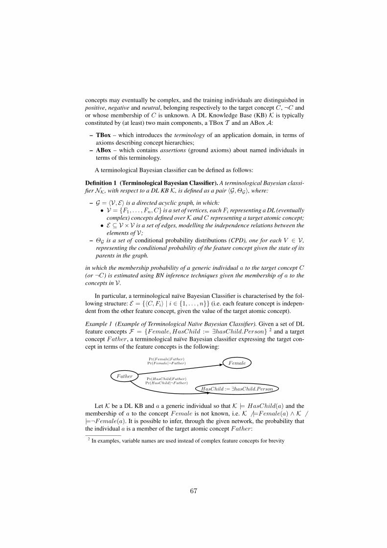
concepts may eventually be complex, and the training individuals are distinguished inpositive, negative and neutral, belonging respectively to the target concept C, ¬C andor whose membership of C is unknown. A DL Knowledge Base (KB) K is typicallyconstituted by (at least) two main components, a TBox T and an ABox A:

– TBox – which introduces the terminology of an application domain, in terms ofaxioms describing concept hierarchies;

– ABox – which contains assertions (ground axioms) about named individuals interms of this terminology.

A terminological Bayesian classifier can be defined as follows:

Definition 1 (Terminological Bayesian Classifier). A terminological Bayesian classi-fier NK, with respect to a DL KB K, is defined as a pair 〈G, ΘG〉, where:

– G = 〈V, E〉 is a directed acyclic graph, in which:• V = F1, . . . , Fn, C is a set of vertices, eachFi representing a DL (eventually

complex) concepts defined overK and C representing a target atomic concept;• E ⊆ V ×V is a set of edges, modelling the independence relations between the

elements of V;– ΘG is a set of conditional probability distributions (CPD), one for each V ∈ V ,

representing the conditional probability of the feature concept given the state of itsparents in the graph.

in which the membership probability of a generic individual a to the target concept C(or ¬C) is estimated using BN inference techniques given the membership of a to theconcepts in V .

In particular, a terminological naıve Bayesian Classifier is characterised by the fol-lowing structure: E = 〈C,Fi〉 | i ∈ 1, . . . , n (i.e. each feature concept is indepen-dent from the other feature concept, given the value of the target atomic concept).

Example 1 (Example of Terminological Naıve Bayesian Classifier). Given a set of DLfeature concepts F = Female,HasChild := ∃hasChild.Person 2 and a targetconcept Father, a terminological naıve Bayesian classifier expressing the target con-cept in terms of the feature concepts is the following:

Pr(Female|Father)Pr(Female|¬Father)

Pr(HasChild|Father)Pr(HasChild|¬Father)

Father

Female

HasChild := ∃hasChild.Person

Let K be a DL KB and a a generic individual so that K |= HasChild(a) and themembership of a to the concept Female is not known, i.e. K 6 |=Female(a) ∧ K 6|=¬Female(a). It is possible to infer, through the given network, the probability thatthe individual a is a member of the target atomic concept Father:

2 In examples, variable names are used instead of complex feature concepts for brevity

67

Pr(Father(a)) =Pr(Father) Pr(HasChild | Father)∑

Father′∈Father,¬FatherPr(Father′) Pr(HasChild | Father′)

;

In the following we define the problem of learning a terminological Bayesian clas-sifier NK given a DL KB K and the training individuals IndC(A):

Definition 2 (Terminological Bayesian Classifier Learning Problem). Our termino-logical naıve Bayesian classifier learning problem consists in finding a network N ∗Kthat maximizes the quality of the network with respect to the training instances and aspecific scoring function; formally:

Given

– a target concept C we aim to learn;– a DL KB K = 〈T ,A〉, where the ABox A contains membership assertions

about individuals and C, while the TBox T does not contain assertions involv-ing C;

– the disjoint sets of of positive, negative and neutral examples for C, denotedwith Ind+

C(A), Ind−C(A) and Ind0C(A), so that:

• ∀a ∈ Ind+C(A) : C(a) ∈ A,

• ∀a ∈ Ind−C(A) : ¬C(a) ∈ A,• ∀a ∈ Ind0

C(A) : C(a) 6∈ A ∧ ¬C(a) 6∈ A;– a scoring function specifying the quality of an induced terminological Bayesian

classifier NK with respect to the samples inIndC(A) =

⋃v∈+,−,0 Ind

vC(A) and a scoring criterion;

Find a network N ∗K maximizing the score function with respect to the samples:

N ∗K ← arg maxNK

score(NK, IndC(A))).

Our search space, to find the optimal network N ∗K, may be too large to exploreexhaustively; therefore our learning algorithm, outlined in Alg. 1, works by greedilysearching the space of features (i.e. DL complex concepts) for the ones that maximizethe score of the induced network, with respect to a scoring function, and incrementallybuilding the resulting network. While the features are added one by one, the search inthe space of DL complex concepts is made through a beam search, employing the ρcl↓closure of the downward refinement operator ρ↓ described in [17].

For each new complex concept being evaluated, the algorithm creates a new set ofconcepts V ′ and finds the optimal structure (under a given set of constraints) E ′ (which,in the case of terminological naıve Bayesian classifiers, is already defined) and thecorresponding maximum likelihood parameters ΘG′ (which may vary depending on theassumptions on the nature of the ignorance model), then scores the new network withrespect to a scoring criterion.

68

Different Assumptions on the Ignorance Model

Let K = 〈T ,A〉 be a DL KB; under OWA, it is not always possible to know if ageneric DL assertion α is or is not entailed by K (i.e. there may be cases in whichK 6 |=α∧K 6 |=¬α). This allows us to characterize our lack of knowledge about concept-memberships through the probability distribution of the ignorance model [23]. Givena generic concept C, a generic individual a and a DL KB K∗, let I be an ignorancemodel from which we extract a fragment of K∗, I(K∗) = K (so that ∀α : K |=α ⇒ K∗ |= α ∧ K∗ |= α 6⇒ K |= α). Let denote NK as a probabilistic modelthat, from a DL KB K, calculates the probability that the concept-membership relationbetween C and a is unknown. We can say that the ignorance model underlying theconcept-membership relation between a and C in K (with respect to a, K∗ and theaforementioned probabilistic model) is:

– MCAR (Missing Completely at Random) – when the probability for such concept-membership to be missing is independent from the knowledge on a available inK∗:Pr(K 6|= C(a) ∧ K 6|= ¬C(a) | K∗) = Pr(K 6|= C(a) ∧ K 6|= ¬C(a));

– MAR (Missing At Random) – when the probability for such concept-membershipto be missing depends on the knowledge on a available in K:Pr(K 6|= C(a) ∧ K 6|= ¬C(a) | K∗) = Pr(K 6|= C(a) ∧ K 6|= ¬C(a) | K);

– NMAR (Not Missing At Random, also referred to as IM, Informatively Missing)– when the probability for such concept-membership to be missing depends on theknowledge on a available in K∗:Pr(K 6|= C(a) ∧ K 6|= ¬C(a) | K∗) 6= Pr(K 6|= C(a) ∧ K 6|= ¬C(a) | K).

Algorithm 1 Algorithm for Learning Terminological Bayesian ClassifiersRequire: DL KB K = 〈T ,A〉, Concept Start, Beam Width w,

Search depth d, Maximum concept description length maxLen,Positive, Negative, Neutral training individuals IndC(A);

Ensure: NK = 〈G, ΘG〉,G = 〈V ← C, E ← ∅〉;1: repeat2: Best← ∅;Beam← Start;NewBeam← ∅;3: repeat4: for c ∈ Beam do5: for c′ ∈ ρcl↓ (c) | |c′| ≤ min(|c|+ d,maxLen) do6: N ′K ← optimalNetwork(V ∪ c′, IndC(A));7: s′ ← score(N ′K, IndC(A));8: NewBeam← NewBeam ∪ 〈N ′K, s′〉;9: end for

10: end for11: Best← arg max〈N ′K,s′〉(s

′ : 〈N ′K, s′〉 ∈ NewBeam ∪ Best);12: Beam← selectFrom(NewBeam,w);NewBeam← ∅;13: until stopping criterion on Beam;14: NK ← N ′K : 〈N ′K, s′〉 = Best;15: until stopping criterion onNK;

69

Specifically, in our algorithm, the outer loop (lines 1-15) greedily searches for anew (complex) concept definition whose addition increases the network’s quality on thegiven sample instances (determined by a scoring function score). The search throughthe space of concept definitions is performed in the inner loop (lines 3-13) through abeam search: starting from a beginning concept Start, for each refinement level, allrefinements up to a given length are memorized in a priority queue NewBeam (sortedaccording to the score associated to the network generated by adding them to the setof feature concepts) from which only the k with the highest score are selected, by theselection function selectFrom, to be refined in the next iteration.

The functions optimalNetwork and score are used, respectively, to find the opti-mal Bayesian network structure between the nodes in the network (eventually under aset of constraints, like in the naıve Bayes case or some of its extensions) and for scoringa classifier (to compare its effectiveness with others). However, those two functions aresensitive to the assumptions made about the ignorance model.

When the assumed ignorance model is MCAR, we are allowed to use an approachcalled available case analysis [15], in which we build an unbiased estimator of thenetwork parameters, based only on available knowledge. A scoring function we realisedfor such case is the network’s log-likelihood on training data, calculated only on positiveand negative training individuals, ignoring the available knowledge about the concept-membership relations between such individuals and the target concept C, and definedas:

L(NK | IndC(A)) = log Pr(NK) +∑

a∈Ind+C(A)

log Pr(C(a) | NK) +∑

a∈Ind−C(A)

log Pr(¬C(a) | NK);

Another approach we implemented consisted in ranking both positive and negativetraining individuals a according to P (C(a) | NK), and then calculating the area un-der the Precision-Recall curve using different acceptance thresholds.

Under the naıve Bayes assumption, there is no need to perform a search for find-ing the optimal network, since the structure is already fixed (each node except the targetconcept node has only one parent, i.e. the target concept node); otherwise, finding a net-work structure which is optimal under some criterion (e.g. the BIC score [15]) may re-quire an exhaustive search in the space of possible structures. However, tree-augmentednaıve Bayesian networks (which allow for a tree structure among feature nodes), it ispossible to efficiently compute the optimal structure employing the method in [12],making it appealing for real-life applications requiring efficiency and scalability.

In the MAR case, a possible solution for learning models accounting for missingknowledge is to use the Expectation-Maximization (EM) algorithm, MCMC samplingor the gradient ascent method [15]. We use EM to learn terminological naıve Bayesianclassifiers from MAR data. In our approach, outlined in Alg. 2, we first heuristicallyestimate network’s parameters by only using available data; then, in order to find themaximum likelihood parameters with respect to both observed and missing knowledge,we consider individuals whose membership to a particular concept description D is notknown as several fractional individuals belonging, with different weights (correspond-ing to the posterior probability of their class membership), to both the components Dand ¬D.

70

Formally, the EM algorithm for parameters learning explores the space of possibleparameters through an iterative hill-climbing search, converging to a (local) maximumlikelihood estimate of the unknown parameters, where the (log-)likelihood (which wealso use as scoring criterion) is defined as follows:

L(NK | IndC(A)) = log Pr(NK) +∑

a∈Ind0C(A)

∑

C′∈C,¬Clog Pr(C ′(a) | NK) Pr(C ′ | NK)

+∑

a∈Ind+C(A)

log Pr(C(a) | NK) +∑

a∈Ind−C(A)

log Pr(¬C(a) | NK);

At each iteration, the EM algorithm applies the following two steps:

– Expectation step – using available data and the current network parameters, cal-culate a distribution over possible completions for the missing knowledge;

– Maximization step – considering each possible completion as a fully availabledata case (weighted by its probability), calculate next parameters using (weighted)frequency counting.

In our use of the EM algorithm, the E-step calculates the concept-membership pos-terior probability (inferencing through the network) of each individual whose concept-membership relation in unknown, thus completing the data through so called expectedcounts. Then, the M-step calculates a new estimate of the network’s conditional prob-ability distributions by using expected counts, maximizing the log-likelihood of bothavailable and missing data with respect to a network NK.

About finding optimal structures for networks with less restrictions on their struc-ture (such as tree-augmented naıve BNs or unrestricted BNs) from MAR data, it ispossible to employ the Structural EM (SEM) algorithm [11]. In SEM, the maximiza-tion step is performed both in the space of structures G and in the space of parametersΘG , by first searching a better structure and then the best parameters associated to thegiven structure; it can be proven that, if the search procedure finds a structure that isbetter than the one used in the previous iteration with respect to e.g. the BIC score, thenthe structural EM algorithm will monotonically improve the score.

When knowledge is NMAR, it is generally possible to extend the probabilisticmodel to produce one where the MAR assumption holds; e.g. if a feature concept Fifollows a NMAR ignorance model, with respect to a generic individual a and a DLKB K, we can consider its observability as an additional variable (e.g. Yi = 0 iffK 6|= Fi(a) ∧ K 6|= ¬Fi(a), Yi = 1 otherwise) in our probabilistic model, so thatFi’s ignorance model satisfies the MAR assumption (since its missingness depends onan always observable variable).

An alternate solution is recurring to robust Bayesian estimation [20] (RBE), to learnconditional probability distributions without making any sort of assumption about thenature of the missing data. RBE finds probability intervals instead of single probabilityvalues, obtained by taking in account all the possible fillings of the missing knowledge;the width of inferred intervals is therefore directly proportional to the quantity of miss-ing knowledge considered during the learning process. To score each new induced net-work, we employ the framework proposed in [26] to compare credal networks, while

71

Algorithm 2 Outline for our implementation of the EM algorithm for parameter learn-ing in a terminological Bayesian classifier assuming the underlying ignorance model isMAR.function ExpectedCounts(NK, IndC(A))

1: NK = 〈G, ΘG〉,G = 〈V, E〉;2: for Xi ∈ V do3: for 〈xi, πxi〉 ∈ vals(Xi, parents(Xi)) do4: n(xi, πxi) contains the expected count for (Xi = xi, parents(Xi) = πxi)5: n(xi, πxi)← 0;6: end for7: end for8: for a ∈ IndC(A) do9: for Xi ∈ V do

10: for 〈xi, πxi〉 ∈ vals(Xi, parents(Xi)) do11: Each expected count n(xi, πxi) is obtained summing out the probability assign-

ments to the concept memberships (Xi = xi, parents(Xi) = πxi) for each indi-vidual, calculated using the background knowledge K and, if they are only partiallyknown, inferring through the networkNK

12: n(xi, πxi)← n(xi, πxi) + Pr(xi, πxi | NK);13: end for14: end for15: end for16: return n(xi, πxi) | Xi ∈ V, 〈xi, πxi〉 ∈ vals(Xi, parents(Xi));function ExpectationMaximization(N 0

K, IndC(A))

1: The network was first initialized with arbitrary heuristic parameters Θ0G

2: N 0K = 〈G, Θ0

G〉,G = 〈V, E〉;3: t← 0;4: repeat5: n(xi, πxi) ← ExpectedCounts(NK, IndC(A));6: for Xi ∈ V do7: for 〈xi, πxi〉 ∈ vals(Xi, parents(Xi)) do8: θt+1

G (xi, πxi)← n(xi,πxi)∑

x′i∈vals(Xi)

n(x′i,πxi);

9: end for10: end for11: t← t+ 1;12: N t

K = 〈G, ΘtG〉;13: The EM loop ends when improvements to the network’s log-likelihood go below a cer-

tain threshold14: until L(N t

K = 〈G, ΘtG)〉 | IndC(A))− L(N t−1K = 〈G, Θt−1

G 〉 | IndC(A)) ≤ τ ;15: return N t

K;

72

we do not have implemented yet a method to search for structures other than naıveBayesian.

Example 2 (Example of Terminological Naıve Bayesian Classifier using Robust BayesianEstimation). The following is a terminological naıve Bayesian classifier using robustBayesian estimation for inferring posterior probability intervals in presence of NMARknowledge. In this networks, conditional probability tables associated to each node con-tain probability intervals instead of probability values, each defined by its upper andlower bound.

[Pr(Female|Father),Pr(Female|Father)][Pr(Female|¬Father),Pr(Female|¬Father)]

[Pr(HasChild|Father),Pr(HasChild|Father)][Pr(HasChild|¬Father),Pr(HasChild|¬Father)]

Fa := Father

Fe := Female

HC := ∃hasChild.Person

Inference, using such network, can be performed as follows – given a generic indi-vidual a and given that K |= HC(a), the posterior probability interval that a is a mem-ber of Fa is represented by the probability interval [Pr(Fa | HC),Pr(Fa | HC)],where:

Pr(Fa(a)) = Pr(Fa | HC) =Pr(HC | Fa)Pr(Fa)

Pr(HC | Fa)Pr(Fa) + Pr(HC | ¬Fa)Pr(¬Fa);

Pr(Fa(a)) = Pr(Fa | HC) =Pr(HC | Fa)Pr(Fa)

Pr(HC | Fa)Pr(Fa) + Pr(HC | ¬Fa)Pr(¬Fa);

4 Conclusions and Future Work

We presented a Statistical Relational Learning method designed for learning termino-logical naıve Bayesian classifiers, a ML method based on the naıve Bayes assumptionfor estimating the probability that a generic individual belongs to a certain target con-cept, given its membership relation to an induced set of complex Description Logicconcepts. We gave a characterisation of the lack of knowledge that may be introducedby the OWA depending on the underlying ignorance model, and handled such missingknowledge under different assumptions on the nature of missing knowledge itself (i.e.Missing Completely at Random, Missing at Random or Informatively Missing). In thefuture, we aim at estimating computationally the ignorance model followed by eachfeature, at developing new methods to exploit the potential information contained inknowledge’s missingness and evaluate our methods’ effectiveness on real world ontolo-gies.

References

[1] OWL 2 Web Ontology Language Direct Semantics (October 2009), http://www.w3.org/TR/owl2-direct-semantics/

73

[2] Berners-Lee, T., Hendler, J., Lassila, O.: The semantic web. Scientific American 284(5),34–43 (May 2001)

[3] Bicer, V., et al.: Relational kernel machines for learning from graph-structured rdf data. In:Antoniou, G., et al. (eds.) ESWC (1). LNCS, vol. 6643, pp. 47–62. Springer (2011)

[4] Caruana, R., Niculescu-Mizil, A.: An empirical comparison of supervised learning algo-rithms. In: ICML2006. pp. 161–168. ACM, New York, NY, USA (2006)

[5] Corani, G., Zaffalon, M.: Naive credal classifier 2: an extension of naive bayes for deliver-ing robust classifications. In: DMIN. pp. 84–90 (2008)

[6] d’Amato, C., Fanizzi, N., Esposito, F.: Query answering and ontology population: an in-ductive approach. In: ESWC 2008. pp. 288–302. Springer (2008)

[7] Domingos, P., et al.: Uncertainty reasoning for the semantic web i. chap. Just Add Weights:Markov Logic for the Semantic Web, pp. 1–25. Springer (2008)

[8] Domingos, P., Pazzani, M.J.: On the optimality of the simple bayesian classifier under zero-one loss. Machine Learning 29(2-3), 103–130 (1997)

[9] Fanizzi, N., et al.: Reduce: A reduced coulomb energy network method for approximateclassification. In: Aroyo, L., et al. (eds.) ESWC. pp. 323–337. Springer (2009)

[10] Fanizzi, N., D’Amato, C., Esposito, F.: Learning with kernels in description logics. In: ILP2008. pp. 210–225. Springer (2008)

[11] Friedman, N.: The Bayesian structural EM algorithm. In: UAI 1998. pp. 129–138. MorganKaufmann Publishers Inc., San Francisco, CA (1998)

[12] Friedman, N., Geiger, D., Goldszmidt, M., Provan, G., Langley, P., Smyth, P.: Bayesiannetwork classifiers. In: Machine Learning. pp. 131–163 (1997)

[13] Getoor, L., Taskar, B.: Introduction to Statistical Relational Learning (Adaptive Computa-tion and Machine Learning). The MIT Press (2007)

[14] Kiefer, C., et al.: Adding Data Mining Support to SPARQL via Statistical Relational Learn-ing Methods. In: ESWC 2008. LNCS, vol. 5021, pp. 478–492. Springer (2008)

[15] Koller, D., Friedman, N.: Probabilistic Graphical Models: Principles and Techniques. MITPress (2009)

[16] Laskey, K.J., Laskey, K.B.: Uncertainty reasoning for the world wide web: Report on theurw3-xg incubator group. In: Bobillo, F., et al. (eds.) URSW. CEUR Workshop Proceed-ings, vol. 423. CEUR-WS.org (2008)

[17] Lehmann, J., Hitzler, P.: Concept learning in description logics using refinement operators.Mach. Learn. 78, 203–250

[18] Luna, J.E.O., Cozman, F.G.: An algorithm for learning with probabilistic description logics.In: Baader, F., Calvanese, D., McGuinness, D.L., Nardi, D., Patel-Schneider, P.F. (eds.)URSW. CEUR Workshop Proceedings, vol. 527, pp. 63–74. CEUR-WS.org (2009)

[19] Pearl, J.: Probabilistic reasoning in intelligent systems: networks of plausible inference.Morgan Kaufmann Publishers Inc., San Francisco, CA, USA (1988)

[20] Ramoni, M., Sebastiani, P.: Robust learning with missing data. Mach. Learn. 45, 147–170(October 2001)

[21] Richardson, M., Domingos, P.: Markov logic networks. Mach. Learn. 62, 107–136 (Febru-ary 2006)

[22] Rodrigues De Morais, S., Aussem, A.: Exploiting data missingness in bayesian networkmodeling. In: IDA 2009. pp. 35–46. Springer (2009)

[23] Rubin, D.B.: Inference and missing data. Biometrika 63(3), 581–592 (1976)[24] Tresp, V., et al.: Uncertainty reasoning for the semantic web i. chap. Towards Machine

Learning on the Semantic Web, pp. 282–314. Springer (2008)[25] Tresp, V., Huang, Y., Bundschus, M., Rettinger, A.: Materializing and querying learned

knowledge. In: IRMLeS 2009 (2009)[26] Zaffalon, M., Corani, G., Maua, D.: Utility-based accuracy measures to empirically evalu-

ate credal classifiers. In: ISIPTA 2011. pp. 401–410. Innsbruck (2011)

74

A Distribution Semantics for ProbabilisticOntologies

Elena Bellodi, Evelina Lamma, Fabrizio Riguzzi, and Simone Albani

ENDIF – University of Ferrara, Via Saragat 1, I-44122, Ferrara, Italyelena.bellodi,evelina.lamma,fabrizio.riguzzi@unife.it

simone.albani@student.unife.it

Abstract. We present DISPONTE, a semantics for probabilistic ontolo-gies that is based on the distribution semantics for probabilistic logic pro-grams. In DISPONTE each axiom of a probabilistic ontology is annotatedwith a probability. The probabilistic theory defines thus a distributionover normal theories (called worlds) obtained by including an axiom ina world with a probability given by the annotation. The probability of aquery is computed from this distribution with marginalization. We alsopresent the system BUNDLE for reasoning over probabilistic OWL DLontologies according to the DISPONTE semantics. BUNDLE is basedon Pellet and uses its capability of returning explanations for a query.The explanations are encoded in a Binary Decision Diagram from whichthe probability of the query is computed.

1 Introduction

Representing probabilistic knowledge and reasoning with it is fundamental inorder to realize the full vision of the Semantic Web, due to the ubiquity of un-certainty in the real world and on the Web [24]. Various authors have advocatedthe use of probabilistic ontologies, see e.g. [17], and many proposals have beenput forward for allowing ontology languages, and OWL in particular, to representuncertainty.

Similarly, in the field of logic programming, there has been much work onintroducing uncertainty in the programs. Among the various proposals, the dis-tribution semantics [22] has emerged as one of the most effective approaches andit underlies many languages such as PRISM [22], ICL [19], Logic Programs withAnnotated Disjunctions [26] and ProbLog [3]. In this semantics a probabilisticlogic program defines a probability distribution over a set of normal logic pro-grams (called worlds). The distribution is extended to a joint distribution overworlds and queries; the probability of a query is obtained from this distributionby marginalization. In general, the problem of integrating logic and probabilityhas been much studied lately, with proposals such as Markov Logic [20], MultiEntity Bayesian Networks [12] and Probabilistic Relational Models [10].

In this paper we propose to apply this approach to ontology languages and,in particular, to the OWL DL fragment, that is based on the description logicSHOIN (D). However, the approach is applicable in principle to any description

75

logic. We called the approach DISPONTE for “DIstribution Semantics for Prob-abilistic ONTologiEs” (Spanish for “get ready”). The idea is to annotate eachaxiom of a theory with a probability and assume that each axiom is indepen-dent of the others. A probabilistic theory defines thus a distribution over normaltheories (worlds) obtained by including an axiom in a world with a probabilitygiven by the annotation. The probability of a query is again computed from thisdistribution with marginalization.

We also present the system BUNDLE for “Binary decision diagrams for Un-certain reasoNing on Description Logic thEories” that performs inference overprobabilistic OWL DL ontologies. BUNDLE uses the inference techniques de-veloped for probabilistic logic programs under the distribution semantics [8,21]and, in particular, the use of Binary Decision Diagrams (BDDs) for encodingexplanations to queries and for computing their probability.

BUNDLE is based on the Pellet reasoner [23] for OWL DL and exploits itscapability of returning explanations for queries in the form of a set of sets ofaxioms from which BUNDLE builds a BDD for computing the probability. Inthis way we provide an effective reasoning system for DISPONTE.

The paper is organized as follows. Section 2 describes the distribution seman-tics for logic programs while Section 3 presents DISPONTE. Section 4 illustratesBUNDLE and Section 5 discusses current limitations of DISPONTE and BUN-DLE. Section 6 describes related works while Section 7 concludes the paper.

2 The Distribution Semantics in Probabilistic LogicProgramming

The probabilistic logic programming languages based on the distribution se-mantics differ in the way they define the distribution over logic programs. Eachlanguage allows probabilistic choices among atoms in clauses. Let us considerProbLog [3] which is the language with the simplest syntax. A ProbLog pro-gram T is composed of a normal logic program TC and a set of probabilisticfacts TP . Each probabilistic fact is of the form pi :: Fi. where pi is a probability(i.e. pi ∈ [0, 1]) and Fi is a atom. This means that every grounding of Fi is aBoolean random variable that assumes true value with probability pi and falsewith probability 1− pi.

Let us call TF the set of atoms obtained by removing the probabilistic an-notation from the probabilistic facts. Let us consider the case in which TC ∪ TFdoes not contain function symbols so that its Herbrand base is finite. Let us callground(T ) the grounding of a normal program T . Since there are no functionsymbols, ground(TC ∪TF ) is finite and so is the grounding ground(TF ) obtainedby grounding the probabilistic atoms with constants from the Herbrand universeof TC ∪ TF . So each probabilistic fact Fi has a finite set of groundings.

A substitution is a set of couples V/c where V is a variable and c is a constant.A substitution θj is applied to a logic atom F , indicated with Fθj , by replacingthe variables in the substitution with constants. A substitution θj is groundingfor logic atom F if Fθj is ground. Suppose that a grounding is obtained with

76

the substitution θj : Fiθj corresponds to a Boolean random variable Xij that isindependent of the others.

Example 1. The following ProbLog program T encodes a very simple model ofthe development of an epidemic or pandemic:

C1 = epidemic : −flu(X), epid(X), cold.C2 = pandemic : −flu(X), \+ epid(X), pand(X), cold.C3 = flu(david).C4 = flu(robert).F1 = 0.7 :: cold.F2 = 0.6 :: epid(X).F3 = 0.3 :: pand(X).This program models the fact that if somebody has the flu and the climate

is cold there is the possibility that an epidemic or a pandemic arises. We areuncertain whether the climate is cold but we know for sure that David andRobert have the flu. epid(X) and pand(X) can be considered as ”probabilisticactivators” of the effects in the head given that the causes (flu(X) and cold)are present. \+ epid(X) means the negation of epid(X).

Fact F1 has only one grounding so there is a single Boolean variable X11. FactF2 has two groundings, epid(david) and epid(robert) so there are two Booleanrandom variables X21 and X22. F3 also has two groundings so there are twoBoolean random variables X31 and X32.

In order to present the distribution semantics, let us first give some definitions.An atomic choice is a selection of a value for a grounding of a probabilisticfact F and is represented by the triple (Fi, θj , k) where θj is a substitutiongrounding Fi and k ∈ 0, 1. A set of atomic choices κ is consistent if (Fi, θj , k) ∈κ, (Fi, θj ,m) ∈ κ ⇒ k = m, i.e., only one truth value is selected for a groundfact. A composite choice κ is a consistent set of atomic choices. The probabilityof composite choice κ is P (κ) =

∏(Fi,θj ,1)∈κ pi

∏(Fi,θj ,0)∈κ(1 − pi). A selection

σ is a total composite choice (one atomic choice for every grounding of everyprobabilistic fact). A selection σ identifies a normal logic program wσ called aworld in this way: wσ = TC ∪ Fiθj |(Fi, θj , 1) ∈ σ. The probability of wσ isP (wσ) = P (σ) =

∏(Fi,θj ,1)∈κ pi

∏(Fi,θj ,0)∈κ(1 − pi). Since ground(TF ) is finite

the set of worlds is finite: WT = w1, . . . , wm and P (w) is a distribution overworlds:

∑w∈WT

P (w) = 1. A world wσ is compatible with a composite choice κif κ ⊆ σ

We can define the conditional probability of a query Q given a world asP (Q|w) = 1 if w |= Q and 0 otherwise. This allows to define a joint distributionof the query and the worlds P (Q,w) by using the product rule of the theory ofprobability: P (Q,W ) = P (Q|w)P (w). The probability of Q can then be obtainedfrom the joint distribution by the sum rule (marginalization over Q):

P (Q) =∑

w∈WT

P (Q,w) =∑

w∈WT

P (Q|w)P (w) =∑

w∈WT :w|=QP (w) (1)

In Example 1, T has 5 Boolean random variables and thus 32 worlds. The queryepidemic is true in 5 of them and its probability is P (epidemic) = 0.588.

77

It is often unfeasible to find all the worlds where the query is true so inferencealgorithms find instead explanations for the query [8,21] , i.e. composite choicessuch that the query is true in all the worlds that are compatible with them . Forexample, κ1 = (F2, X/david, 1), (F1, , 1) is an explanation for the queryepidemic and so is κ2 = (F2, X/robert, 1), (F1, , 1).

Each explanation κ identifies a set of worlds, those that are compatible withit, and a set of explanations K identifies the set ωK of worlds compatible withone of its explanations (ωK = wσ|κ ∈ K,κ ⊆ σ). A set of explanations K iscovering for a query Q if every world in which Q is true is in ωK . For example,K = κ1, κ2 is covering for the query epidemic.

The probability of a query can thus be computed from a covering set ofexplanations for the query by computing the probability of the Boolean formula

B(Q) =∨

κ∈K

∧

(Fi,θj ,1)∈κXij

∧

(Fi,θj ,0)∈κ¬Xij (2)

For Example 1, the formula is B(epidemic) = X11 ∧X21 ∨X11 ∧X22.Explanations however, differently from possible worlds, are not necessarily

mutually exclusive with respect to each other, so the probability of the query cannot be computed by a summation as in (1). In fact computing the probabilityof a DNF formula of independent Boolean random variables is a #P-completeproblem [25]. The method that was found to be the most efficient up to nowconsists in building a Binary Decision Diagram for the formula and using adynamic programming algorithm on the BDD [8,21]. A BDD is a rooted graphthat has one level for each variable. Each node n has two children, a 0-child anda 1-child. The leaves store either 0 or 1. Given values for all the variables, aBDD can be used to compute the value of the formula by traversing the graphstarting from the root, following the edges corresponding to the variables valuesand returning the value associated to the leaf that is reached. The BDD forExample 1 is shown in Figure 1.

X21 n1

X22 n2

X11 n3

1 0

Fig. 1. BDD for Example 1.

A BDD performs a Shannon expansion of the Boolean formula f(X), sothat if X is the variable associated to the root level of a BDD, the formulaf(X) can be represented as f(X) = X ∧ fX(X) ∨ ¬X ∧ f¬X(X) where fX(X)

78

(f¬X(X)) is the formula obtained by f(X) by setting X to 1 (0). Now the twodisjuncts are mutually exclusive and the probability of f(X) can be computed asP (f(X)) = P (X)P (fX(X))+(1−P (X))P (f¬X(X)) Figure 2 shows the functionProb that implements the dynamic programming algorithm for computing theprobability of a formula encoded as a BDD.

Fig. 2. Function Prob: computation of the probability of a Boolean formula encodedas a BDD with root node.

1: function Prob(node)2: if node is a terminal then3: return value(node) . value(node) is either 0 or 14: else5: let X be v(node) . v(node) is the variable associated to node6: return Prob(child0(node)) ·(1− P (X))+Prob(child1(node))·P (X)7: end if8: end function

Languages with non-binary choices such as Logic Programs with AnnotatedDisjunctions can be handled by encoding the choices with binary variables [21].

3 The DISPONTE Semantics for Probabilistic Ontologies

DISPONTE assigns a semantics to probabilistic ontologies following the ap-proach of the distribution semantics for probabilistic logic programs. It definesa probability distribution over non-probabilistic ontologies called worlds. Thisprobability distribution is extended to a joint distribution of the worlds and aquery and the probability of the query is obtained by marginalization.

The probabilistic ontologies we consider associate to each axiom of the on-tology a Boolean random variable that indicates whether the axiom is presentin a world. A probabilistic ontology is thus a set of annotated axioms of the form

pi :: Ai (3)

or of unannotated axioms of the form Ai, for i = 1, . . . , n, where pi is theprobability with which axiom Ai is included in a world. Let us call OA the setA1, . . . , An and Xi the Boolean random variable associated to axiom Ai. EachXi is independent of every Xj with i 6= j. The probability of each Xi of beingtrue is pi. If the pi :: annotation is omitted for an axiom, we assume that theaxiom is certain, i.e., that it has probability 1.

A world w is obtained by sampling a value for Xi for every axiom Ai of OAand by including Ai in w if Xi = 1. Since the random variables for the differentaxioms are independent, the probability P (w) of w is obtained as:

P (w) =∏

Ai∈wpi

∏

Aj∈OA\w(1− pj)

79

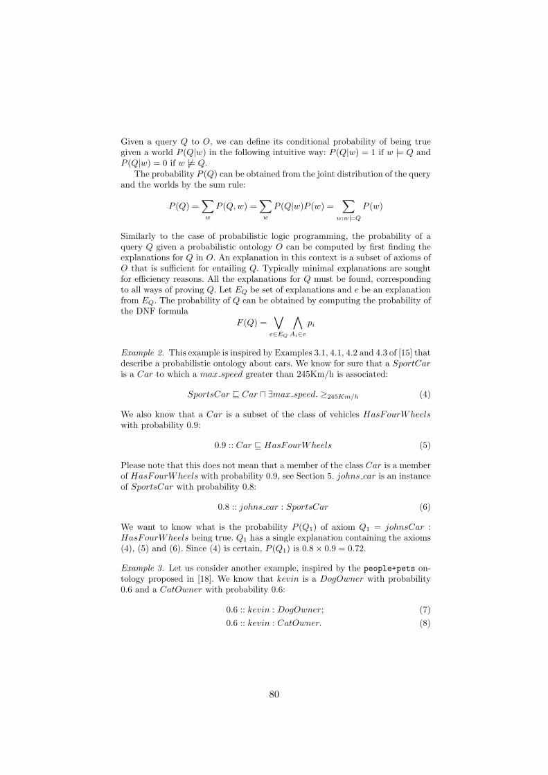
Given a query Q to O, we can define its conditional probability of being truegiven a world P (Q|w) in the following intuitive way: P (Q|w) = 1 if w |= Q andP (Q|w) = 0 if w 6|= Q.

The probability P (Q) can be obtained from the joint distribution of the queryand the worlds by the sum rule:

P (Q) =∑

w

P (Q,w) =∑

w

P (Q|w)P (w) =∑

w:w|=QP (w)

Similarly to the case of probabilistic logic programming, the probability of aquery Q given a probabilistic ontology O can be computed by first finding theexplanations for Q in O. An explanation in this context is a subset of axioms ofO that is sufficient for entailing Q. Typically minimal explanations are soughtfor efficiency reasons. All the explanations for Q must be found, correspondingto all ways of proving Q. Let EQ be set of explanations and e be an explanationfrom EQ. The probability of Q can be obtained by computing the probability ofthe DNF formula

F (Q) =∨

e∈EQ

∧

Ai∈epi

Example 2. This example is inspired by Examples 3.1, 4.1, 4.2 and 4.3 of [15] thatdescribe a probabilistic ontology about cars. We know for sure that a SportCaris a Car to which a max speed greater than 245Km/h is associated:

SportsCar v Car u ∃max speed. ≥245Km/h (4)

We also know that a Car is a subset of the class of vehicles HasFourWheelswith probability 0.9:

0.9 :: Car v HasFourWheels (5)

Please note that this does not mean that a member of the class Car is a memberof HasFourWheels with probability 0.9, see Section 5. johns car is an instanceof SportsCar with probability 0.8:

0.8 :: johns car : SportsCar (6)

We want to know what is the probability P (Q1) of axiom Q1 = johnsCar :HasFourWheels being true. Q1 has a single explanation containing the axioms(4), (5) and (6). Since (4) is certain, P (Q1) is 0.8× 0.9 = 0.72.

Example 3. Let us consider another example, inspired by the people+pets on-tology proposed in [18]. We know that kevin is a DogOwner with probability0.6 and a CatOwner with probability 0.6:

0.6 :: kevin : DogOwner; (7)0.6 :: kevin : CatOwner. (8)

80

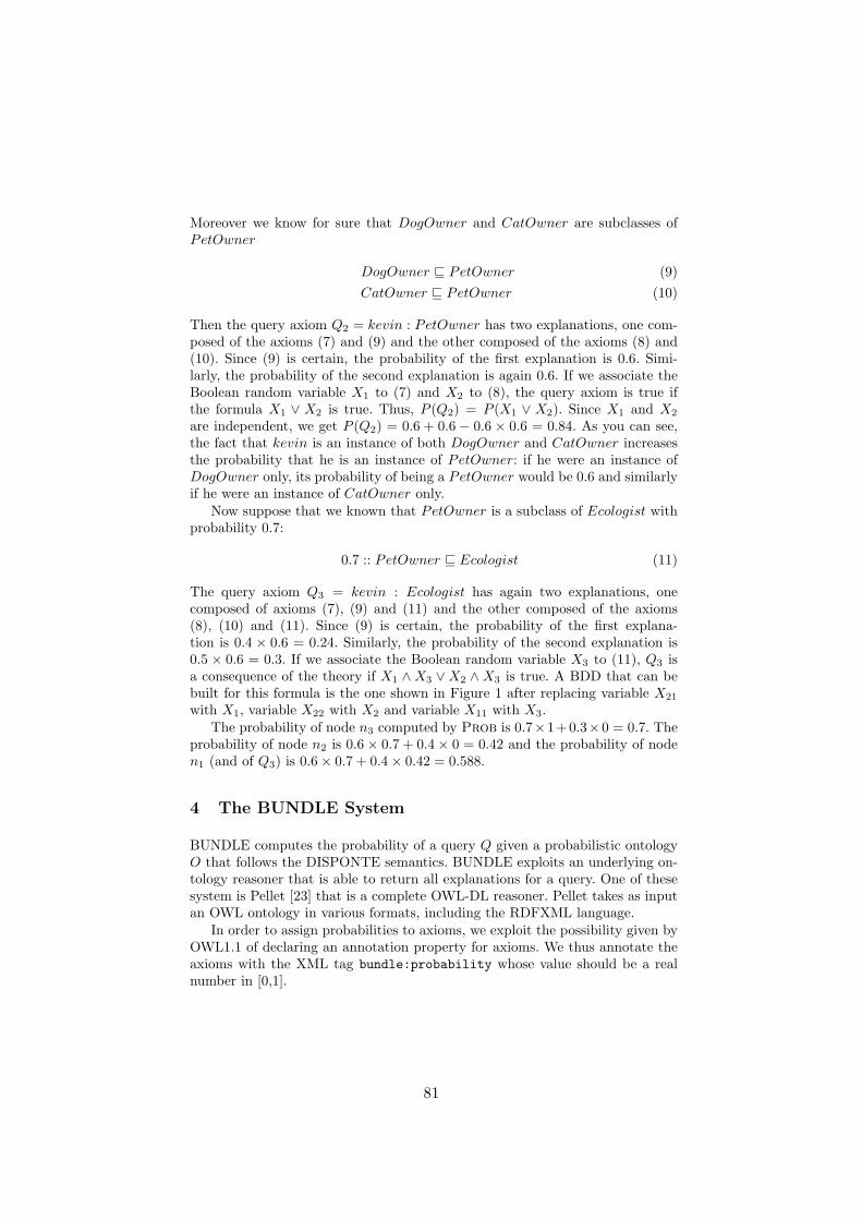
Moreover we know for sure that DogOwner and CatOwner are subclasses ofPetOwner

DogOwner v PetOwner (9)CatOwner v PetOwner (10)

Then the query axiom Q2 = kevin : PetOwner has two explanations, one com-posed of the axioms (7) and (9) and the other composed of the axioms (8) and(10). Since (9) is certain, the probability of the first explanation is 0.6. Simi-larly, the probability of the second explanation is again 0.6. If we associate theBoolean random variable X1 to (7) and X2 to (8), the query axiom is true ifthe formula X1 ∨ X2 is true. Thus, P (Q2) = P (X1 ∨ X2). Since X1 and X2

are independent, we get P (Q2) = 0.6 + 0.6 − 0.6 × 0.6 = 0.84. As you can see,the fact that kevin is an instance of both DogOwner and CatOwner increasesthe probability that he is an instance of PetOwner: if he were an instance ofDogOwner only, its probability of being a PetOwner would be 0.6 and similarlyif he were an instance of CatOwner only.

Now suppose that we known that PetOwner is a subclass of Ecologist withprobability 0.7:

0.7 :: PetOwner v Ecologist (11)

The query axiom Q3 = kevin : Ecologist has again two explanations, onecomposed of axioms (7), (9) and (11) and the other composed of the axioms(8), (10) and (11). Since (9) is certain, the probability of the first explana-tion is 0.4 × 0.6 = 0.24. Similarly, the probability of the second explanation is0.5 × 0.6 = 0.3. If we associate the Boolean random variable X3 to (11), Q3 isa consequence of the theory if X1 ∧X3 ∨X2 ∧X3 is true. A BDD that can bebuilt for this formula is the one shown in Figure 1 after replacing variable X21

with X1, variable X22 with X2 and variable X11 with X3.The probability of node n3 computed by Prob is 0.7×1+0.3×0 = 0.7. The

probability of node n2 is 0.6× 0.7 + 0.4× 0 = 0.42 and the probability of noden1 (and of Q3) is 0.6× 0.7 + 0.4× 0.42 = 0.588.

4 The BUNDLE System

BUNDLE computes the probability of a query Q given a probabilistic ontologyO that follows the DISPONTE semantics. BUNDLE exploits an underlying on-tology reasoner that is able to return all explanations for a query. One of thesesystem is Pellet [23] that is a complete OWL-DL reasoner. Pellet takes as inputan OWL ontology in various formats, including the RDFXML language.

In order to assign probabilities to axioms, we exploit the possibility given byOWL1.1 of declaring an annotation property for axioms. We thus annotate theaxioms with the XML tag bundle:probability whose value should be a realnumber in [0,1].

81

BUNDLE takes as input two RDFXML files, one containing the ontologyand one containing the annotations. For Example 3, the ontology file containsthe following definition of PetOwner:

<owl:Class rdf:about="#PetOwner"><rdfs:subClassOf>

<owl:Class rdf:about="#Ecologist" /></rdfs:subClassOf>

</owl:Class>

The annotation file contains the annotation for the above axiom in the followingform:

<owl11:Axiom><rdf:subject rdf:resource="#PetOwner"/><rdf:predicate rdf:resource="&rdfs;subClassOf"/><rdf:object rdf:resource="#Ecologist"/><bundle:probability>0.6</bundle:probability>

</owl11:Axiom>

BUNDLE first uses the annotation file for building a data structure PMapthat associates axioms with their probability. In order to do so, axioms arefirst converted to strings. We use the Manchester syntax to obtain a stringrepresentation of an axiom.

Then BUNDLE uses the Explain function of Pellet to compute explanationsfor a query axiom. BUNDLE thus accepts all the forms of query axioms thatare accepted by Pellet’s Explain function, namely subclass, instance, propertyvalue, theory inconsistency and class unsatisfiability.

Pellet returns the explanations for the query in the form of a set of sets ofaxioms. Then BUNDLE performs a double loop over the set of explanations andover the set of axioms in each explanation in which it builds a BDD representingthe set of explanations. To manipulate BDDs we used the JavaBDD library1

that provides a Java interface to the major BDD libraries such as CUDD2.Outside the outer loop, two data structures are initialized: V arAxAnn is an

array that maintains the association between Boolean random variables (whoseindex is the array index) and axioms together with their probability, and BDDrepresents the set of explanations. BDD is initialized to the BDD representingthe zero Boolean function. Then the outer loop is entered in which BDDE isinitialized to the BDD representing the one Boolean function. In the inner loopthe axioms of an explanation are considered one by one. Each axiom is firstlooked up in PMap to get its probability. If NULL is returned this means thatthis is a certain axiom and it does not need to be considered anymore. Thenthe axiom is searched for in V arAxAnn to see if it has already been assigneda random variable. If not, a cell is added to V arAxAnn to store the axiomwith its probability. At this point we know the axiom’s position i in V arAxAnn1 http://javabdd.sourceforge.net/2 http://vlsi.colorado.edu/~fabio/CUDD/

82

and so the index of its Boolean variable Xi. We obtain a BDD representingXi = 1 and we conjoin it with BDDE. At the end of the inner loop the BDD forthe current explanation, BDDE, is disjoined with BDD. After the two cycles,function Prob of Figure 2 is called over BDD and its result is returned to theuser.

BUNDLE has been implemented in Java and will be available for downloadfrom http://sites.unife.it/bundle. It has been successfully tested on vari-ous examples, including those of Section 3.

5 Discussion

The probabilistic knowledge that can be expressed with the DISPONTE seman-tics is epistemic by nature, namely it represents degrees of belief in the axiomsrather that statistical information. While this is reasonable for many axioms, forsubclass and subproperty axioms one may want to express statistical informa-tion, for example with a probabilistic subclass axiom p :: A v B one may wantto express the fact that a random individual of A has probability p of belongingto B. The DISPONTE semantics, instead, interpret the axioms as stating thatA v B is true with probability p. The difference is that, if two individuals i and jbelong to class A, the probability that they both belong to B in the DISPONTEsemantics is p while with a statistical interpretation is p × p. Thus statisticalinformation can be used to define a degree of partial overlap between classes.Extending DISPONTE to take account of this case is possible, it requires todefine a probability distribution over models rather than over theories.

However, to reason with such knowledge, the inference engine must be modi-fied in its inference procedure and cannot be used as a black box as in BUNDLE.In fact, BUNDLE assigns a single Boolean random variable to the axiom A v B,while with a statistical interpretation a different Boolean random variable mustbe assigned to each assertion that an individual of class A belongs to class B.We leave this extension for future work.

Another limitation of BUNDLE is the use of the OWL 1.1 Axiom constructto specify probabilities. This seems to restrict the kind of axioms on whichprobabilities can be placed, since the object of the RDF triple does not allowcomplex class expressions. However this limitation can be overcome by defining anew class which is equivalent to the complex class expression and using the newclass name in the RDF triple. In the future we plan to investigate the possibilityof annotating the axioms directly in the ontology file.

As regards the complexity of reasoning on DISPONTE, it is equal to the com-plexity of the underlying description logic plus the #P complexity of computingthe probability of a DNF formula of independent Boolean random variables, as-suming the cost of keeping track of explanations during inference is negligible.Thus, the problem of inference in DISPONTE remains decidable if it was so inthe underlying description logic.

83

6 Related Work

Our work differs from previous work in many respects. [6] proposed an exten-sion of the description logic ALC that is able to express statistical informationon the terminological knowledge such as partial concept overlapping. Similarly,[11] presents a probabilistic description logic based on Bayesian networks thatdeals with statistical terminological knowledge. As illustrated in Section 5, cur-rently we are not able to express statistical terminological knowledge but it ispossible to extend the semantics to do so. Differently from us, [6,11] do notallow probabilistic assertional knowledge about concept and role instances. [7]allows assertional knowledge about concept and role instances together with sta-tistical terminological knowledge and combines the resulting probability distri-butions using cross-entropy minimization. In the future we plan to compare theDISPONTE semantics extended with statistical information with this approach.

[4] proposed a probabilistic extension of OWL that admits a translation intoBayesian networks. The semantics that is proposed assigns a probability distri-bution P (i) over individuals, i.e.

∑i P (i) = 1, and assigns a probability to a class

C as P (C) =∑i∈C P (i), while we assign a probability distribution over theo-

ries. PR-OWL [2,1] is an upper ontology that provides a framework for buildingprobabilistic ontologies. It allows to use the first-order probabilistic logic MEBN[12] for representing uncertainty in ontologies. The use of a full fledged first-orderprobabilistic logic distringuishes this work from ours, where we tried to providea minimal extension to description logics.

A different approach to the combination of description logic with probabilityis taken by [5,13,14] where the authors use probabilistic lexicographic entailmentfrom probabilistic default reasoning. The logics proposed in these papers allowboth terminological probabilistic knowledge as well as assertional probabilisticknowledge about instances of concepts and roles. PRONTO [9] is one of thesystems that allows to perform inference in this semantics.

Similary to [7], the terminological knowledge is interpreted statistically whilethe assertional knowledge is interpreted epistemically by assigning degrees ofbeliefs to assertions, thus differing from our current treatment of terminologicalknowledge. Moreover it also allows to express default knowledge about con-cepts that can be overridden in subconcepts and whose semantics is given byLehmann’s lexicographic default entailment.

These works are based on Nilsson’s probabilistic logic [16] where a proba-bilistic interpretation Pr defines a probability distribution over the set of in-terpretations I. The probability of a logic formula φ according to Pr, denotedPr(φ), is the sum of all Pr(I) such that I ∈ I and I |= φ.

A probabilistic knowledge base K is a set of probabilistic formulas of theform φ ≥ p. A probabilistic interpretation Pr satisfies φ ≥ p iff Pr(φ) ≥ p. Prsatisfies K, or Pr is a model of K, iff Pr satisfies all F ∈ K. We say φ ≥ p is atight logical consequence of K iff p is the infimum of Pr(φ) subject to all modelsPr of K. Computing tight logical consequences from probabilistic knowledgebases can be done by solving a linear optimization problem.

84

Nilsson’s probabilistic logic differs from the distribution semantics: while aprobabilistic knowledge base in Nilsson’s logic may have multiple models thatare probabilistic interpretations, a probabilistic program under the distributionsemantics has a single model that defines a single distribution over interpreta-tions. Also, while in Nilsson’s logic we want to compute the lowest p such thatPr(φ) ≥ p holds for all Pr, in the distribution semantics we want to compute psuch that P (φ) = p. Nilsson’s logic complexity is lower than the #P complexityof the distribution semantics.

In fact Nilsson’s logic allows weaker conclusions than the distribution se-mantics. For example, consider a probabilistic program composed of 0.4 :: a. and0.5 :: b. and a probabilistic knowledge base composed of a ≥ 0.4 and b ≥ 0.5. Thedistribution semantics allows to say that P (a∨b) = 0.7, while with Nilsson’s logicthe lowest p such that Pr(a ∨ b) ≥ p holds is 0.5. This is due to the fact that inthe distribution semantics the probabilistic atoms are considered independent,which allows to make stronger conclusions. However, note that this does notrestrict expressiveness as you can specify with the distribution semantics anyjoint probability distribution over the atoms of the Herbrand base interpretedas Boolean random variables, possibly introducing new random facts if needed.

Alternative approaches to modeling imperfect and incomplete knowledge inontologies are based on fuzzy logic. A good survey of these approaches is pre-sented in [15].

7 Conclusions

We have presented the semantics DISPONTE for probabilistic ontologies thatis inspired by the distribution semantics of probabilistic logic programming. Wehave also presented the system BUNDLE that is able to compute the probabilityof queries from an uncertain OWL DL ontology.

In the future, we plan to extend DISPONTE to take into account statisticalterminological knowledge and improve the way in which the input to BUNDLEis specified.

References

1. Carvalho, R.N., Laskey, K.B., Costa, P.C.: PR-OWL 2.0 - bridging the gap toOWL semantics. In: International Workshops on Uncertainty Reasoning for theSemantic Web (2010)

2. Costa, P.C.G., Laskey, K.B., Laskey, K.J.: Pr-owl: A bayesian ontology languagefor the semantic web. In: International Workshops on Uncertainty Reasoning forthe Semantic Web. vol. 5327, pp. 88–107. Springer (2008)

3. De Raedt, L., Kimmig, A., Toivonen, H.: ProbLog: A probabilistic Prolog andits application in link discovery. In: International Joint Conference on ArtificialIntelligence. pp. 2462–2467 (2007)

4. Ding, Z., Peng, Y.: A probabilistic extension to ontology language OWL. In: HawaiiInternational Conference On System Sciences. IEEE (2004)

85

5. Giugno, R., Lukasiewicz, T.: P-SHOQ(D): A probabilistic extension of SHOQ(D)for probabilistic ontologies in the semantic web. In: European Conference on Logicsin Artificial Intelligence. LNCS, vol. 2424, pp. 86–97. Springer (2002)

6. Heinsohn, J.: Probabilistic description logics. In: Conference on Uncertainty inArtificial Intelligence. pp. 311–318. Morgan Kaufmann (1994)

7. Jaeger, M.: Probabilistic reasoning in terminological logics. In: International Con-ference on Principles of Knowledge Representation and Reasoning. pp. 305–316(1994)

8. Kimmig, A., Demoen, B., Raedt, L.D., Costa, V.S., Rocha, R.: On the implemen-tation of the probabilistic logic programming language problog. Theory Pract. Log.Program. 11(2-3), 235–262 (2011)

9. Klinov, P.: Pronto: A non-monotonic probabilistic description logic reasoner. In:European Semantic Web Conference. LNCS, vol. 5021, pp. 822–826. Springer(2008)

10. Koller, D.: Probabilistic relational models. In: International Workshop on InductiveLogic Programming. LNCS, vol. 1634, pp. 3–13. Springer (1999)

11. Koller, D., Levy, A.Y., Pfeffer, A.: P-classic: A tractable probablistic descriptionlogic. In: National Conference on Artificial Intelligence. pp. 390–397 (1997)

12. Laskey, K.B., da Costa, P.C.G.: Of starships and klingons: Bayesian logic for the23rd century. In: Conference in Uncertainty in Artificial Intelligence. pp. 346–353.AUAI Press (2005)

13. Lukasiewicz, T.: Probabilistic default reasoning with conditional constraints. Ann.Math. Artif. Intell. 34(1-3), 35–88 (2002)

14. Lukasiewicz, T.: Expressive probabilistic description logics. Artif. Intell. 172(6-7),852–883 (2008)

15. Lukasiewicz, T., Straccia, U.: Managing uncertainty and vagueness in descriptionlogics for the semantic web. J. Web Sem. 6(4), 291–308 (2008)

16. Nilsson, N.J.: Probabilistic logic. Artif. Intell. 28(1), 71–87 (1986)17. Obrst, L., McCandless, D., Stoutenburg, S., Fox, K., Nichols, D., Prausa, M.,

Sward, R.: Evolving use of distributed semantics to achieve net-centricity. In: AAAIFall Symposium (2007)

18. Patel-Schneider, P.F., Horrocks, I., Bechhofer, S.: Tutorial on OWL (2003), http://www.cs.man.ac.uk/~horrocks/ISWC2003/Tutorial/

19. Poole, D.: Abducing through negation as failure: stable models within the inde-pendent choice logic. J. of Log. Program. 44(1-3), 5–35 (2000)

20. Richardson, M., Domingos, P.: Markov logic networks. Machine Learning 62(1-2),107–136 (2006)

21. Riguzzi, F.: Extended semantics and inference for the Independent Choice Logic.Log. J. IGPL 17(6), 589–629 (2009)

22. Sato, T.: A statistical learning method for logic programs with distribution seman-tics. In: International Conference on Logic Programming. pp. 715–729. MIT Press(1995)

23. Sirin, E., Parsia, B., Grau, B.C., Kalyanpur, A., Katz, Y.: Pellet: A practicalOWL-DL reasoner. J. Web Sem. 5(2), 51–53 (2007)

24. URW3-XG: Uncertainty reasoning for the World Wide Web, final report, http://www.w3.org/2005/Incubator/urw3/XGR-urw3/

25. Valiant, L.G.: The complexity of enumeration and reliability problems. SIAM J.Comp. 8(3), 410–421 (1979)

26. Vennekens, J., Verbaeten, S., Bruynooghe, M.: Logic programs with annotateddisjunctions. In: International Conference on Logic Programming. LNCS, vol. 3131,pp. 195–209. Springer (2004)

86

Semantic Link Prediction through ProbabilisticDescription Logics

Kate Revoredo1, Jose Eduardo Ochoa Luna2, and Fabio Gagliardi Cozman2

1 Departamento de Informatica Aplicada, UnirioAv. Pasteur, 458, Rio de Janeiro, RJ, Brazil

2 Escola Politecnica, Universidade de Sao Paulo,Av. Prof. Mello Morais 2231, Sao Paulo - SP, Brazil

katerevoredo@uniriotec.br,eduardo.ol@gmail.com,fgcozman@usp.br

Abstract. Predicting potential links between nodes in a network is aproblem of great practical interest. Link prediction is mostly based ongraph-based features and, recently, on approaches that consider the se-mantics of the domain. However, there is uncertainty in these predictions;by modeling it, one can improve prediction results. In this paper, we pro-pose an algorithm for link prediction that uses a probabilistic ontologydescribed through the probabilistic description logic crALC. We use anacademic domain in order to evaluate this proposal.

1 Introduction

Many social, biological, and information systems can be well described by net-works, where nodes represent objects (individuals), and links denote the rela-tions or interactions between nodes. Predicting a possible link in a network isan interesting issue that has recently gained attention, due to the growing inter-est in social networks. For instance, one may be interested on finding potentialfriendship between two persons in a social network, or a potential collaborationbetween two researchers. Thus link prediction [12, 20] aims at predicting whethertwo nodes (i.e. people) should be connected given that we know previous infor-mation about their relationships or interests. A common approach is to exploitthe network structure, where numerical information about nodes is analyzed[12, 20, 9]. However, knowledge about the objects represented in the nodes canimprove prediction results. For instance consider that the researchers Joe andMike do not have a publication in common, thus they do not share a link in acollaboration network. Moreover, graph features do not indicate a potential linkbetween them. However, they have published in the same journal and they bothteach the same course in their respectively universities. This information can bean indication of a potential collaboration between them. Given this, approachesthat are based on the semantics related to the domain of the objects representedby the nodes [21, 18] have been proposed. In some of them, an ontology modelingthe domain and the object interests were used in the prediction task.

However, there is uncertainty in such predictions. Often, it is not possibleto guarantee the relationship between two objects (nodes). This is maybe due

87

to the fact that information about the domain is incomplete. Thus, it wouldbe interesting if link prediction approaches could handle the probability of alink conditioned on the information about the domain. In our example, knowingthat the probability of the relationship between Joe and Mike conditioned onthe knowledge of them publishing in the same journal and teaching the samecourse is high implies a link between them in the network; otherwise, a link isnot suggested. In graph-based approaches, probabilistic models learned throughmachine learning algorithms were used for link prediction. Some examples ofprobabilistic models are Probabilistic Relational Model (PRM) [6], ProbabilisticEntity Relationship Model (PERM) [7] and Stochastic Relational Model (SRM)[22]. On approaches based on semantic we claim that ontologies must be usedto model the domain. Therefore, to model uncertainty, probabilistic approaches,such as probabilistic ontologies, must be considered.

An ontology can be represented through a description logic [2], which is typi-cally a decidable fragment of first-order logic that tries to reach a practical bal-ance between expressivity and complexity. To encode uncertainty, a probabilisticdescription logic (PDL) must be contemplated. The literature contains a numberof proposals for PDLs [8, 10, 19, 13]. In this paper we adopt a recently proposedPDL, called Credal ALC (crALC) [4, 16, 5], that extends the popular logic ALC[2]. In crALC one can specify sentences such as P (Professor|Researcher) = 0.4,indicating the probability that an element of the domain is a Professor giventhat it is a Researcher. These sentences are called probabilistic inclusions. Exactand approximate inference algorithms that deal with probabilistic inclusionshave been proposed [4, 5], using ideas inherited from the theory of RelationalBayesian Networks (RBN)[11].

In this paper, we propose to use a probabilistic ontology defined with thePDL crALC for semantic link prediction.

The paper is organized as follows. Section 2 reviews basic concepts of PDLsand crALC. Section 3 presents our algorithm for semantic link prediction throughthe PDL crALC. Experiments are discussed in Section 4, and Section 5 con-cludes the paper.

2 Probabilistic Description Logics and crALC

Description logics (DLs) form a family of representation languages that are typi-cally decidable fragments of first order logic (FOL) [2]. Knowledge is expressedin terms of individuals, concepts, and roles. The semantic of a description isgiven by a domain D (a set) and an interpretation ·I (a functor). Individualsrepresent objects through names from a set NI = a, b, . . .. Each concept in theset NC = C,D, . . . is interpreted as a subset of a domain D. Each role in theset NR = r, s, . . . is interpreted as a binary relation on the domain.

Several probabilistic descriptions logics (PDLs) have appeared in the litera-ture. Heinsohn [8], Jaeger [10] and Sebastiani [19] consider probabilistic inclusionaxioms such as PD(Professor) = α, meaning that a randomly selected object is aProfessor with probability α. This characterizes a domain-based semantics: prob-

88

abilities are assigned to subsets of the domain D. Sebastiani also allows inclusionssuch as P (Professor(John)) = α, specifying probabilities over the interpretationsthemselves. For example, one interprets P (Professor(John)) = 0.001 as assigning0.001 to be the probability of the set of interpretations where John is a Professor.This characterizes an interpretation-based semantics.

The PDL crALC is a probabilistic extension of the DL ALC that adopts aninterpretation-based semantics. It keeps all constructors of ALC, but only allowsconcept names on the left hand side of inclusions/definitions. Additionally, incrALC one can have probabilistic inclusions such as P (C|D) = α or P (r) = βfor concepts C and D, and for role r. If the interpretation of D is the wholedomain, then we simply write P (C) = α. The semantics of these inclusions isroughly (a formal definition can be found in [5]) given by:

∀x ∈ D : P (C(x)|D(x)) = α,

∀x ∈ D, y ∈ D : P (r(x, y)) = β.

We assume that every terminology is acyclic; no concept uses itself. This as-sumption allows one to represent any terminology T through a directed acyclicgraph. Such a graph, denoted by G(T ), has each concept name and role nameas a node, and if a concept C directly uses concept D, that is if C and D appearrespectively in the left and right hand sides of an inclusion/definition, then Dis a parent of C in G(T ). Each existential restriction ∃r.C and value restriction∀r.C is added to the graph G(T ) as nodes, with an edge from r and C to eachrestriction directly using it. Each restriction node is a deterministic node in thatits value is completely determined by its parents.

Example 1. Consider a terminology T1 with concepts A,B,C,D. SupposeP (A) = 0.9,B v A,C v B t ∃r.D, P (B|A) = 0.45, P (C|B t ∃r.D) = 0.5, andP (D|∀r.A) = 0.6. The last three assessments specify beliefs about partial overlapamong concepts. Suppose also P (D|¬∀r.A) = ε ≈ 0 (conveying the existence ofexceptions to the inclusion of D in ∀r.A). Figure 1 depicts G(T ).

Fig. 1. G(T ) for terminology T in Example 1 and its grounding for domain D = a, b.

89

The semantics of crALC is based on probability measures over the space ofinterpretations, for a fixed domain. Inferences, such as P (Ao(a0)|A) for an ABoxA, can be computed by propositionalization and probabilistic inference (for exactcalculations) or by a first order loopy propagation algorithm (for approximatecalculations) [5].

3 Link Prediction by using crALCIn this section we describe how to apply the PDL crALC for semantic linkprediction. We borrowed some syntax from the graph-based approach whereeach node (a person in a social network) is represented by A,B,C, and we areinterested in defining whether a link between A and B is suitable given there isno link between these nodes. Interests between the nodes are modeled through aprobabilistic ontology represented by the PDL crALC. The prediction link taskcan be described as:

Given:• a network defining relationship between objects;• an ontology represented by crALC describing the domain of the objects;• the ontology role that defines the semantic of the relationship between

objects;• the ontology concept that describes the network objects.

Find:• a revised network defining relationship between objects.

The proposed algorithm for link prediction receives a network of a specificdomain. For instance, in a collaboration network the nodes represent researchersand the relationship can have the semantic ”has a publication with” or ”is ad-vised by”. Therefore, the ontology represented by crALC describes the domainof publications between researchers, having concepts like Researcher, Publication,StrongRelatedResearcher and NearCollaborator and roles like hasPublication,hasSameInstitution and sharePublication. This ontology can be learned automat-ically through a learning algorithm as the ones proposed in [15, 17]. Thus, thenodes represent instances of one of the concepts described in the PDL crALCand the semantic of the links is described by one of the roles in the PDL crALC.These concept and role must be informed as inputs to the proposed algorithm.The link prediction algorithm is described in Algorithm 1.

The algorithm starts looking for all pairs of instances of the concept C definedas the concept that provides the semantic for the network nodes. For each pairit checks whether the corresponding nodes exist in the network (this can beimproved by exploring graph-based properties). If not the probability of thelink is calculated through the probability of the defined role conditioned onevidence. The evidence is provided by the instances of the ontology. As manyinstances the ontology have the better is the inference performed. The inferenceis performed through the Relational Bayesian network build from ontology O. Ifthe probability inferred is greater than a threshold then the corresponding link

90

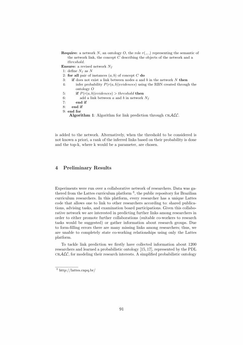
Require: a network N , an ontology O, the role r( , ) representing the semantic ofthe network link, the concept C describing the objects of the network and athreshold.

Ensure: a revised network Nf1: define Nf as N2: for all pair of instances (a, b) of concept C do3: if does not exist a link between nodes a and b in the network N then4: infer probability P (r(a, b)|evidences) using the RBN created through the

ontology O5: if P (r(a, b)|evidences) > threshold then6: add a link between a and b in network Nf7: end if8: end if9: end for

Algorithm 1: Algorithm for link prediction through crALC.

is added to the network. Alternatively, when the threshold to be considered isnot known a priori, a rank of the inferred links based on their probability is doneand the top-k, where k would be a parameter, are chosen.

4 Preliminary Results

Experiments were run over a collaborative network of researchers. Data was ga-thered from the Lattes curriculum platform 3, the public repository for Braziliancurriculum researchers. In this platform, every researcher has a unique Lattescode that allows one to link to other researchers according to: shared publica-tions, advising tasks, and examination board participations. Given this collabo-rative network we are interested in predicting further links among researchers inorder to either promote further collaborations (suitable co-workers to researchtasks would be suggested) or gather information about research groups. Dueto form-filling errors there are many missing links among researchers; thus, weare unable to completely state co-working relationships using only the Lattesplatform.

To tackle link prediction we firstly have collected information about 1200researchers and learned a probabilistic ontology [15, 17], represented by the PDLcrALC, for modeling their research interests. A simplified probabilistic ontology

3 http://lattes.cnpq.br/

91

is given by:

P (Publication) = 0.3P (Board) = 0.33P (sharePublication) = 0.22P (wasAdvised) = 0.05P (hasSameInstitution) = 0.14P (sameExaminationBoard) = 0.31

ResearcherLattes ≡ Personu(∃hasPublication.Publicationu∃advises.Person u ∃participate.Board)

P (PublicationCollaborator | Researcher u ∃sharePublication.Researcher) = 0.91P (SupervisionCollaborator | Researcher u ∃wasAdvised.Researcher) = 0.94P (SameInstitution | Researcher u ∃hasSameInstitution.Researcher) = 0.92P (SameBoard | Researcheru

∃sameExaminationBoard.Researcher) = 0.92P (NearCollaborator | Researcher u ∃sharePublication.∃hasSameInstitution.

∃sharePublication.Researcher) = 0.95FacultyNearCollaborator ≡ NearCollaborator

u ∃sameExaminationBoard.Researcher

P (NullMobilityResearcher | Researcher u ∃wasAdvised.∃hasSameInstitution.Researcher) = 0.98

StrongRelatedResearcher ≡ Researcheru (∃sharePublication.Researcher u∃wasAdvised.Researcher)

InheritedResearcher ≡ Researcheru (∃sameExaminationBoard.Researcher u∃wasAdvised.Researcher)

In this probabilistic ontology concepts and probabilistic inclusions denote mu-tual research interests. For instance, a PublicationCollaborator inclusion refers toResearchers who shares a Publication, thus relates two nodes (Researcher) in a col-laboration graph. Therefore, the concept Researcher and the role sharePublicationare inputs to the algorithm we proposed in Algorithm 1.

To perform inferences and therefore to obtain link predictions, a proposition-alization step (a resulting relational Bayesian network) is required.

In addition, a collaboration graph, based on shared publications, was alsodefined. Statistical information was computed accordingly. Figure 2 depicts col-laborations among 303 researchers. Several relationships and clusterings can alsobe observed.

If we carefully inspect this collaboration graph (Figure 3 shows a subgraphobtained from Figure 2) we could be interested, for instance, in predicting linksamong researchers from different groups.

Thus, in Figure 3 one could further investigate whether a link between re-searcher R (red octagon node) and the researcher B (blue polygon node) issuitable. In order to infer this, the probability of a possible link between R and

92

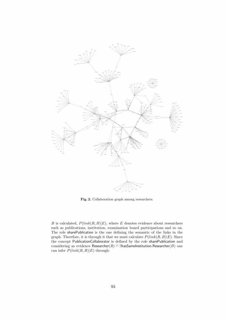
Aldo Tonso

Andreas Karoly Gombert

1

Celso Ricardo Denser Pamboukian

1

Irene Fernandes

1

Mari Cleide Sogayar

1

Felipe Santiago Chambergo Alcalde

1

Valéria Mendes Rodas

1

Patricia Barros dos Santos

1

Soraia Attie Calil Jorge

1

Fabiano Henrique Marques

1

Carlos Augusto Pereira

1

Ari José Scattone Ferreira

1

Mateus Meneghesso da Conceição

1

Amilton SinatoraAndre Paulo Tschiptschin1

Celso Pupo Pesce

1

Linilson Rodrigues Padovese

1

Roberto Mart ins de Souza

1

Cristian Camilo Viáfara Arango

1

Deniol Katsuki Tanaka

1

Giuseppe Pintaúde

1

Wilson Luiz Guesser

1

Marcio Gustavo Di Vernieri Cuppari

1

Ricardo Fuoco

1

Miguel Angelo de Carvalho

1

Ivan Gilberto Sandoval Falleiros

1

Marcelo Nelson Páez Carreño

1

Renato Rufino Xavier

1

Célia Aparecida Lino dos Santos

1

Inés Pereyra

1

Daniel Rodrigues

1

Julio Cesar Klein das Neves

1

Newton Kiyoshi Fukumasu

1

Helio Goldenstein

1

Paulo Roberto Mei

1

Andre Fabio Kohn

1

Fernando Jose Gomes Landgraf

1

Idalina Vieira Aoki

1

Neusa Alonso-Falleiros

1

1

Dairo Hernán Mesa Grajales

1

1

1

11

1

1

Ailton Camargo

1

Abel André Cândido Recco

1

Stephan Wolynec

1

Flavio Beneduce Neto

1

Anna Helena Reali COSTA

Antonio Carlos Silva Costa Teixeira

Antonio Carlos Vieira Coelho

Antonio Domingues de Figueiredo

Carmen Cecilia Tadini

Hercílio Gomes de Melo

1

1

Jorge Andrey Wilhelms Gut

1

Maria Elena Santos Taqueda

1

Pedro de Alcântara Pessôa Filho

1

Jose Mauricio Pinto

1

Carmen Cecilia Tadini1

El izabete Wenzel de Menezes

1

Susy Frey Sabato

1

Javier Telis Romero

1

Flavio Cesar Cunha Galeazzo

1

Aurea Yuki Sugai

1

Suzana Caetano da Si lva Lannes

1

Pedro Vitoriano de Oliveira

1

Pricila Veiga dos Santos

1

Patrícia Ponce

1

Claudio Augusto Oller do Nascimento

1

Reinaldo Giudici

1

Roberto Guardani

1

Osvaldo Chiavone Filho

1

Isabela Bellot de Souza Will

1Frank Herbert Quina

1

Antonio Esio Bresciani

1

Airton Jose de Luna

1

Marco Giulietti

1

Cinthia Tiemi Muranaka

1

Amilcar Machulek Junior

1

Sylvana Cavedon Presti Migliavacca

1

Douglas Gouvêa

1

Henrique Kahn

1

Jose Deodoro Trani Capocchi

1

Samuel Marcio Toffoli

1

Edson Roberto Leite

1

Ing Hwie Tan

1

Marcos Cramer Esteves

1

Reginaldo Muccillo

1

José Alberto Cerri

1

Jefferson Bettini

1

Carlos Renato Rambo

1

Victor Carlos Pandolfelli1

Ricardo Hauch Ribeiro de Castro

1

Emílio Carlos Nelli Silva

Emilio Del Moral Hernandez

1

1

11

1

1

Rodrigo Magnabosco

1

Carlos Shinit i Muranaka

1

Fábio Cardoso Chagas

1

Walman Benicio de Castro

1

Julio Carlos Teixeira

1

Raimundo Carlos Silvério Freire

1

Suzilene Real Janasi

1

Frank Patrick Missell

1

Geraldo Caixeta Guimarães

1

Alexandre Magno Barros de Freitas

1

Fernando Josepett i Fonseca

John Paul Hempel Lima

1

Gerson dos Santos

1

Maria Aparecida Godoy Soler Pajanian

1

Joao Paulo Sinnecker

1

Leni Campos Akcelrud

1

Paulo Sergio Santos

1

Rodrigo Fernando Bianchi

1

Marystela Ferreira

1

Adnei Melges de Andrade

1

Rodrigo Andrade Martinez

1

Paulo Cesar de Morais

1

Antônio Otávio de Toledo Patrocínio

1

Ely Antonio Tadeu Dirani

1

Rinaldo Gregorio Filho

1

Antonio Riul Júnior

1

Vitor Angelo Fonseca Deichmann

1

Miguel Alexandre Novak

1

Patr icia Alexandra Antunes

1

Everaldo Carlos Venancio

1

Fernando Rebouças Stucchi

Flávio Buiochi

Francisco Ferreira Cardoso

1

Henrique Lindenberg Neto

1

Márcia Terra da Silva

1

Mauro Zilbovicius

1

Mercia Maria Semensato Bottura de Barros

1

Silvio Burrattino Melhado

1

Adriana Gouveia Rodrigo

1Erika Paiva Tenório de Holanda

1

Fred Borges da Silva

1

Marco Antônio Penido de Rezende

1

Heliana Comin Vargas

1

Ubiraci Espinelli Lemes de Souza

1

Eliana Kimie Taniguti

1

Adriano Gameiro Vivancos

1

Leonardo Tolaine Massetto

1

Fernando Henrique Sabbat ini

1

Tathyana Moratt i

1

Cláudio Vicente Mitidieri Filho

1

Viviane Miranda Araujo

1

Marcela Paula Maria Zanin Meneguett i

1

Cláudia Nascimento de Jesus

1

Carlos Torres Formoso

1

Fernando Resende

1

1

1

Vanderley Moacyr John

1

1

1

Maria Cristina Motta de Toledo

1

Sérgio Cirelli Angulo

1

Lil ia Mascarenhas Sant Agostino

1

Viviane Carillo Ferrari

1

Helmut Born

1

Giuliana Ratti

1

Wildor Theodoro Hennies

1

1

11

Marina Magnani

1

Marcel Dupret Lopes Barbosa

1

Assis Vicente Benedett i

1

Patr ic ia Hatsue Suegama

1

Risomá Chaves

1

Maysa Terada

1

Isolda Costa

1

Mitiko Saiki

1

Fernando Morais dos Reis

1

Rocio del Pi lar Bendezú Hernández

1

Susana Ines Cordoba de Torresi

1

1

1

1

1

1

1

Henrique Eisi Toma

1

1

1

1

Mônica de Fátima Lobão Granero

1

Ivan Eduardo Chabu

Izabel Fernanda Machado

João Antonio Martino

Luciano Mendes Camillo

1

Michele Rodrigues

1

Rudolf Theoderich Bühler

1

Salvador Pinil los Gimenez

1

Victor Sonnenberg

1

Aparecido Sirley Nicolett

1

Antonio Luis Pacheco Rotondaro

1

Alan Rodrigo Navia

1

Marcello Bellodi

1

Michelly de Souza

1

Marcelo Antonio Pavanello

1

Sebastiao Gomes dos Santos Fi lho1

Milene Galeti

1

José Roberto Cardoso

1

1

Luiz Lebensztajn

1

Roberto Moura Sales

1

Silvio Ikuyo Nabeta

1

Viviane Cristine Silva

1

Jose Jaime da Cruz

1

1

Bernardo Pinheiro de Alvarenga

1

Renato Carlson

1

Maurício Caldora Costa

1

José Augusto Pereira da Silva

1

Wanderlei Marinho da Silva

1

Marcos Antonio Ruggieri Franco

1

Mario Leite Pereira Filho

1

Pedro Pereira de Paula

1

Sérgio Luís Lopes Verardi

1

Yasmara Conceicao De Polli Migliano

1

Antonio Carlos de Jesus Paes

1

Djonny Weinzierl

1

Fabio Henrique Pereira

1

Mauricio Barbosa de Camargo Salles

1

José Roberto Casti lho Piqueira

1

Renato Teodoro Ramos

1

Nilton César Furtado Canto

1

Luiz Henrique Alves Monteiro

1

Vanessa Oliva Araujo

1

José Guilherme de Souza Chaui Mattos Berl inck

1

André Alves Ferreira

1

Henrique Schützer Del Nero

1

Mari lene de Pinho Santos Mazza

1

Ati la Madureira Bueno

1

Iberê Luiz Caldas

1

Julio Cezar Adamowski

Jun Okamoto Junior

Kazuo Nishimoto

1

1

1

Attilio Converti

1 Joao Batista de Almeida e Silva

1

Tiago Martinello

1

Luis Fernando Peffi Ferreira

1 Leoberto Costa Tavares

1

Geraldo Narciso da Rocha Filho

1

André Rolim Baby

1

Elfriede Marianne Bacchi

1Lucia Helena Terra Guerra

1

Cleber Marcos Ribeiro Dias

1

Orestes Marraccini Goncalves

Paulo Carlos Kaminski

Paulo Eigi Miyagi

Paulo Sérgio Licciardi Messeder Barreto

Pedro Afonso de Oliveira Almeida

Rafael Giuliano Pileggi

1 Roberto Cesar de Oliveira Romano

1

1

André Rocha Studart

1

Jose de Anchieta Rodrigues

1

Gracinda Marina Castelo da Silva

1

Heloísa Crist ina Fernandes

1

Reinaldo Morabito Neto

1

Jose Renato Coury

1

Murilo Daniel de Mello Innocentini

1

Andrea Murillo Betioli

1

1

11

1

1

Esleide Lopes Casella

1

Tah Wun Song

1

Pedro Henrique Hermes de Araujo

1

Ariovaldo Bolzan

1

Alexandre Eliseu Stourdze Visconti

1

Heizir Ferreira de Castro

1

Fabio Bentes Freire

1

Teresa Cristina Brazil de Paiva

1

1

1

1

1

1

1

1

1

Carlos Eduardo Calmanovici

1

Katia Ribeiro

1

Efraim Cekinski

1

1 1

1

1

Marjorie Benegra

1

Ronaldo Câmara Cozza

1

Sara Aida Rodriguez Pulecio

1

1

1

1

1

1

1

Humberto Naoyuki Yoshimura

1

Raul Gonzalez Lima

1

Jose Daniel Biasoli de Mello

1

Crist iane Ueda

1

Sergio Shiguemi Furuie

1

1

1

Fabiane Bizinella Nardon

1

Eduardo Moacyr Krieger

1

Eduardo Massad

1

Paulo Bandiera Paiva

1

Denis Roberto Zamignani

1

Vivian Rodrigues Fiales

1

Griselda Esther Jara de Garrido

1

Cecil Chow Robilotta

1

Silvia Maria de Souza Selmo

Tulio Nogueira Bittencourt

1

1

Paulo Roberto do Lago Helene

1

João Cyro André

1

Ricardo Amorim Einsfeld

1

Marco Antonio Meggiolaro

1

José Umberto Arnaud Borges

1

Jaime Tupiassú Pinho de Castro

1

Joaquim Bento Cavalcante Neto

1

Eduardo Parente Prado

1

Luiz Fernando Campos Ramos Martha

1

Gilson Fujii1

Luiz Eduardo Teixeira Ferreira

1

Vahan Agopyan

1

1

1

1

1

1

1

1

1

Carina Ulsen

1

1

1

Alex Kenya Abiko

1

1

1Racine Tadeu Araujo Prado

1

1

1

Thiago Melanda Mendes

1

Vanessa Gomes da Si lva

1

Maristela Gomes da Silva

1

Neide Matiko Nakata Sato

1

Arnaldo Manoel Pereira Carneiro

1

Bruno Luís Damineli

1

Artemária Coêlho de Andrade

1

Miguel Aloysio Sattler

1

Brunoro Leite Giordano

1

Anne Komatsu Agopyan

1

Mário Sousa Takeashi

1

Wang Shu Hui

Neylor Antunes Stevo

Renato Seij i Tavares

1

1

1

1

1

1

1

1

1

1

1

1

1

1

1

1

1

1

1

1

1

1

1

1

1

1

1

1

1

Lucas Antonio Moscato

Marcos de Sales Guerra Tsuzuki

1

1

1

1

1

1

1

1

1

1

Guilherme Canuto da Si lva

1

Fig. 2. Collaboration graph among researchers.

B is calculated, P (link(R,B)|E), where E denotes evidence about researcherssuch as publications, institution, examination board participations and so on.The role sharePublication is the one defining the semantic of the links in thegraph. Therefore, it is through it that we must calculate P (link(R,B)|E). Sincethe concept PublicationCollaborator is defined by the role sharePublication andconsidering as evidence Researcher(R) u ∃hasSameInstitution.Researcher(B) onecan infer P (link(R,B)|E) through:

93

Amilton Sinatora

Linilson Rodrigues Padovese

1

Deniol Katsuki Tanaka

1

Giuseppe Pintaúde

1

Wilson Luiz Guesser

1

Marcio Gustavo Di Vernieri Cuppari

1

Ricardo Fuoco

1

Andre Paulo Tschiptschin

1

Miguel Angelo de Carvalho

1

Ivan Gilberto Sandoval Falleiros

1

Celso Pupo Pesce

1

Marcelo Nelson Páez Carreño

1

Renato Rufino Xavier

1

Cristian Camilo Viáfara Arango

1

Célia Aparecida Lino dos Santos

1

Roberto Mart ins de Souza

1

Inés Pereyra

1

Daniel Rodrigues

1

Julio Cesar Klein das Neves

1

Newton Kiyoshi Fukumasu

1

Helio Goldenstein

1

Paulo Roberto Mei

1

Fernando Josepett i FonsecaGerson dos Santos1

Maria Aparecida Godoy Soler Pajanian

1

Joao Paulo Sinnecker

1

Leni Campos Akcelrud

1

Paulo Sergio Santos

1

Rodrigo Fernando Bianchi

1

Marystela Ferreira

1

Adnei Melges de Andrade

1

Rodrigo Andrade Martinez

1

Paulo Cesar de Morais

1

Antônio Otávio de Toledo Patrocínio

1

Ely Antonio Tadeu Dirani

1

Rinaldo Gregorio Filho

1

Antonio Riul Júnior

1

Vitor Angelo Fonseca Deichmann

1

Miguel Alexandre Novak

1

Patr icia Alexandra Antunes

1

Everaldo Carlos Venancio

1

John Paul Hempel Lima

1

Francisco Ferreira Cardoso

Erika Paiva Tenório de Holanda

1

Fred Borges da Silva

1

Marco Antônio Penido de Rezende

1

Heliana Comin Vargas

1

Ubiraci Espinelli Lemes de Souza

1

Eliana Kimie Taniguti

1

Adriano Gameiro Vivancos

1

Mercia Maria Semensato Bottura de Barros

1

Leonardo Tolaine Massetto

1

Fernando Henrique Sabbat ini

1

Tathyana Moratt i

1

Adriana Gouveia Rodrigo

1

Márcia Terra da Silva

1

Anna Helena Reali COSTA

1

Cláudio Vicente Mitidieri Filho

1

Viviane Miranda Araujo

1

Henrique Lindenberg Neto

1

Marcela Paula Maria Zanin Meneguett i

1

Mauro Zilbovicius

1

Cláudia Nascimento de Jesus

1

Carlos Torres Formoso

1

Fernando Resende

1

Silvio Burrattino Melhado

1

José Roberto Cardoso

Renato Carlson

1

Maurício Caldora Costa

1

José Augusto Pereira da Silva

1

Jose Jaime da Cruz

1

Wanderlei Marinho da Silva

1

Marcos Antonio Ruggieri Franco

1

Carlos Shinit i Muranaka

1

Emilio Del Moral Hernandez

1

Luiz Lebensztajn

1

Mario Leite Pereira Filho

1

Pedro Pereira de Paula

1

Sérgio Luís Lopes Verardi

1

Yasmara Conceicao De Polli Migliano

1

Viviane Cristine Silva

1

Antonio Carlos de Jesus Paes

1

Djonny Weinzierl

1

Fabio Henrique Pereira

1

Mauricio Barbosa de Camargo Salles

1

Bernardo Pinheiro de Alvarenga

1

Roberto Moura Sales

1

Silvio Ikuyo Nabeta

1

Ivan Eduardo Chabu

1

Vanderley Moacyr John

1

1

Heloísa Crist ina Fernandes

1

Henrique Kahn

1

Racine Tadeu Araujo Prado

1

Arnaldo Manoel Pereira Carneiro

1

Antonio Carlos Vieira Coelho

1

Thiago Melanda Mendes

1

Neide Matiko Nakata Sato1

Bruno Luís Damineli

1

Artemária Coêlho de Andrade

1

Orestes Marraccini Goncalves

1

Miguel Aloysio Sattler

1

Brunoro Leite Giordano

1

Vanessa Gomes da Si lva

1

Vahan Agopyan

1Anne Komatsu Agopyan

1

Andrea Murillo Betioli

1

Antonio Domingues de Figueiredo

1

Cleber Marcos Ribeiro Dias

1

Sérgio Cirelli Angulo

1

Roberto Cesar de Oliveira Romano

1

Maristela Gomes da Silva

1

Rafael Giuliano Pileggi

1

Alex Kenya Abiko

1

Mário Sousa Takeashi

1

Silvia Maria de Souza Selmo

1

Carina Ulsen

1

Maria Elena Santos Taqueda

1

Fig. 3. Collaboration subgraph.

P (PublicationCollaborator(R) |Researcher(R)u∃hasSameInstitution.Researcher(B)) = 0.57.

If we took a threshold of 0.60, the link between R and B would not beincluded.

One could gain more evidence, such as information about nodes that in-directly connect these two groups (Figure 3), denoted by I1, I2. The inferencewould be

P (PublicationCollaborator(R) |Researcher(R)u∃sharePublication(I1).∃sharePublication(B)u∃sharePublication(I2).∃sharePublication(B)) = 0.65.

Because more information was provided the probability inferred was different.The same threshold now would preserve the link.

Other inferences are possible by considering the suggestion of links betweensurrounding nodes, i.e. nodes directly linked to the two nodes R and B , denotedby R1, . . . , Rk, and B1, . . . , Bn respectively. For each i = 1, ..., k and j = 1, ..., n,calculates P (link(Ri, Rj)|E) and P (link(Bi, Bj)|E).

94

As a rule, if we are interested in discovering whether A and B could be linked,probabilistic inference P (link(A,B)) should be performed.

In a more general framework, graph information could be useful to deal with alarge number of link predictions. Note that graph adjacency allow us to addressprobabilistic inference for promising nodes. In a naive approach, each pair ofnodes in the collaboration graph would be evaluated so, multiple probabilisticrelational Bayesian inference calls would be required.

On the other hand, if graph-based information is used, such naive schemecould be improved. In our approach, two nodes are probabilistically evaluatedif there is a path between them (number of incoming/outgoing edges, numberof mutual friends, node distances are also considered). Thus, numerical graph-based information guides the inference process in the relational Bayesian network(linked to the probabilistic ontology). In addition, other candidates sharing anykind of evidence are also evaluated, i.e., interests based features (linked to onto-logical knowledge) allow us to further explore link prediction.

Alternatively, by completing an overall link predicting task we can devisefurther functionalities to the resulting collaboration network. The resulting graphcan be considered as being a probabilistic network, i.e., probabilities inferred foreach link could be denote strenght of the relationship.

5 Conclusion

We have presented an approach for predicting links that resorts both to graph-based and ontological information. Given a collaborative network, e.g., a socialnetwork, we encode interests and graph features through a crALC probabilisticontology. In order to predict links we resort to probabilistic inference. Prelimi-nary results focused on an academic domain, and we aimed at predicting linksamong researchers. These preliminary results showed the potential of the idea.

Previous combined approaches for link prediction [3, 1] have focused on ma-chine learning algorithms [14]. In such schemes, numerical graph-based featuresand ontology-based features are computed; then both features are input into amachine learning setting where prediction is performed. Differently from suchapproaches, in our work we adopt a generic ontology (instead of a hierarchi-cal ontology, expressing only is-a relationships among interests). Therefore, ourapproach uses more information about the domain to help the prediction.

Acknowledgements

The third author is partially supported by CNPq. The work reported here hasreceived substantial support by FAPESP grant 2008/03995-5.

References

1. W. Aljandal, V. Bahirwani, D. Caragea, and H.W. Hsu. Ontology-aware classifica-tion and association rule mining for interest and link prediction in social networks.

95

In AAAI 2009 Spring Symposium on Social Semantic Web: Where Web 2.0 MeetsWeb 3.0, Standford,CA, 2009.

2. F. Baader and W. Nutt. Basic description logics. In Description Logic Handbook,pages 47–100. Cambridge University Press, 2002.

3. D. Caragea, V. Bahirwani, W. Aljandal, and W. H. Hsu. Ontology-based linkprediction in the livejournal social network. In Symposium on Abstraction, Refor-mulation and Approximation, 2009.

4. F. G. Cozman and R. B. Polastro. Loopy propagation in a probabilistic descrip-tion logic. In Sergio Greco and Thomas Lukasiewicz, editors, Second InternationalConference on Scalable Uncertainty Management, Lecture Notes in Artificial In-telligence (LNAI 5291), pages 120–133. Springer, 2008.

5. F. G. Cozman and R. B. Polastro. Complexity analysis and variational inference forinterpretation-based probabilistic description logics. In Conference on Uncertaintyin Artificial Intelligence, 2009.

6. N. Friedman, L. Getoor, D. Koller, and A. Pfeffer. Learning probabilistic relationalmodels. In Proc. 16th Int. Joint Conference on Artificial Intelligence, pages 1300–1309, 1999.

7. D. Heckerman, C. Meek, and D. Koller. Probabilistic entity-relationship models,prms, and plate models. In In Proceedings of the 21st International Conference onMachine Learning, 2004.

8. J. Heinsohn. Probabilistic description logics. In International Conf. on Uncertaintyin Artificial Intelligence, pages 311–318, 1994.

9. W.H. Hsu, A.L. King, M.S.R. Paradesi, T. Pydimarri, and T. Wneinger. Collab-orative and structural recommendation of friends using weblog-based social net-work analysis. In Proceedings of Computational Approaches to Analysing WebLogs(AAAI), 2006.

10. M. Jaeger. Probabilistic reasoning in terminological logics. In Principals of Know-ledge Representation (KR), pages 461–472, 1994.

11. M. Jaeger. Relational Bayesian networks: a survey. Linkoping Electronic Articlesin Computer and Information Science, 6, 2002.

12. D. Liben-Nowell and J. Kleinberg. The link prediction problem for social net-works. In Proceedings of the twelfth international conference on Information andKnowledge Management, pages 556–559, New York, NY, USA, 2003. ACM.

13. T. Lukasiewicz and U. Straccia. Managing uncertainty and vagueness in descriptionlogics for the semantic web. Web Semant., 6:291–308, November 2008.

14. T. Mitchell. Machine Learning. McGraw-Hill, New York, 1997.

15. J. Ochoa-Luna, K. Revoredo, and F.G. Cozman. Learning sentences and assess-ments in probabilistic description logics. In Bobillo, F., et al. (eds.) Proceedings ofthe 6th International Workshop on Uncertainty Reasoning for the Semantic Web,volume 654, pages 85–96, Shangai, China, 2010. CEUR-WS.org.

16. R. B. Polastro and F. G. Cozman. Inference in probabilistic ontologies with at-tributive concept descriptions and nominals. In 4th International Workshop onUncertainty Reasoning for the Semantic Web (URSW) at the 7th InternationalSemantic Web Conference (ISWC), Karlsruhe, Germany, 2008.

17. K. Revoredo, J. Ochoa-Luna, and F. Cozman. Learning terminologies in proba-bilistic description logics. In Antonio da Rocha Costa, Rosa Vicari, and FlavioTonidandel, editors, Advances in Artificial Intelligence SBIA 2010, volume 6404of Lecture Notes in Computer Science, pages 41–50. Springer / Heidelberg, Berlin,2010.

96

18. M. Sachan and R. Ichise. Using semantic information to improve link predictionresults in network datasets. International Journal of Computer Theory and Enge-neering, 3:71–76, 2011.

19. F. Sebastiani. A probabilistic terminological logic for modelling information re-trieval. In ACM Conf. on Research and Development in Information Retrieval(SIGIR), pages 122–130, 1994.

20. B. Taskar, M. FaiWong, P. Abbeel, and D. Koller. Link prediction in relationaldata. In Proceedings of the 17th Neural Information Processing Systems (NIPS),2003.

21. T. Wohlfarth and R. Ichise. Semantic and event-based approach for link predic-tion. In Proceedings of the 7th International Conference on Practical Aspects ofKnowledge Management, 2008.

22. K. Yu, W. Chu, S. Yu, V. Tresp, and Z. Xu. Stochastic relational models fordiscriminative link prediction. In Proceedings of the Neural Information ProcessingSystems (NIPS), 2006.

97

98

Position Papers

100

Distributed Imprecise Design Knowledgeon the Semantic Web

Julian R. Eichhoff1 and Wolfgang Maass2

1 Furtwangen University, Robert-Gerwig-Platz 1, 78120 Furtwangen, Germanyjulian.eichhoff@hs-furtwangen.de

2 Saarland University, P.O. 15 11 50, 66041 Saarbrucken, Germanywolfgang.maass@iss.uni-saarland.de

Abstract. In this paper we outline a shared knowledge representationbased on RDF. It can be used in a distributed multi-tenant environmentto store design knowledge. These RDF-graphs incorporate all necessaryinformation to instantiate Bayesian network representations of certainproblem solving cases, which are used to support the conceptual designtasks carried out by a salesperson during lead qualification.

1 Introduction

In industries that offer customized goods and services, which meet their cus-tomer’s individual business needs, vendors are often required to employ a con-sultative sales strategy called “solution selling” (cf. [7]). It comprises mainly fourinterdependent processes carried out on a per project basis: requirements defini-tion, customization and integration, deployment, and post-deployment support.The groundwork for these processes is laid by the vendor’s sales force screeningfor potential customers (leads) and assessing their willingness and ability to buya solution. This task is termed “lead qualification”. Lead qualification in solutionselling industries is highly dependent on a salesperson’s individual knowledge ofa lead’s (problem) situation, of goods and services offered by the vendor and itspartners, and of how certain bundles of goods and services may be used for prob-lem solving; we term this design knowledge. But especially external salespersonsare not directly involved in product development at the employing vendor, andthus may have narrow insights on how their work affects downstream processes.Experiences from other salespersons may not be considered due to limited report-ing or inconsequent knowledge reuse. And limited possibilities or rigid policies forinter-organizational communication may exclude design insights from partneringorganizations. To overcome these shortcomings in intra- and inter-organizationaldesign knowledge reuse, we’ve implemented a shared design knowledge reposi-tory based on the Function-Behavior-Structure (FBS) framework [4] and use itfor services which support the design activities during lead qualification.

Xue and Xu [8] suggest a web-accessible distributed database to store designknowledge based on the FBS notation. Like other models that operationalize theFBS framework [2, 6], they follow an entity-relationship approach. However, it

101

would require a significant knowledge engineering effort to continuously main-tain a design model that builds on a highly detailed and formal knowledge rep-resentation (KR), where innovative yet uncertain design beliefs may be left out.Probability theory can provide an adequate framework to model uncertainties indesign decisions [5]. Encouraging approaches that represent probabilistic beliefnetworks by means of semantic models exist in other domains [9, 10]. But to theauthor’s knowledge, there exist no Semantic Web representations of the FBSframework that incorporate uncertainty information, and can be managed in amulti-tenant environment. In [3] we defined a Bayesian Network (BN) represen-tation of the FBS model, termed FBS-BN, which encodes design knowledge asprobability tables. In the following we outline its shared storage in a distributedRDF-Store.

2 Design Knowledge Representation and Storage

A FBS-BN represents a configurational design space for a specific problem-solving situation in form of a Bayesian Network. Discrete random variables areused to describe possible design object configurations in light of the customer’sdemands. Every variable is associated with a certain component of the design ob-ject to serve as characterizing attribute. There are three different variable types:Function variables (F ) represent the purpose for which a solution is designedfor, i.e. goals and constraints of the customer. Structure variables (S) representpossible offerings, i.e. product and service bundles that can be provided by thevendor. Behaviors are mediating concepts between Functions and Structures rep-resenting the actual solution, i.e. how products and services are meant to achievegoals and fulfill constraints. There are three subtypes of Behavior variables: Bevariables describe the solution as expected by the customer; their value is de-rived from Function variables. Bs variables represent the solution as offered bythe vendor; their value is derived from Structure variables. And Bc variablesare used for comparing the match of Be and Bs. The design knowledge abouthow Functions, Behaviors and Structures affect each other is encoded in formof conditional probability distributions (CPDs). These CPDs represent a set ofpropositions of the form “if concept X is in state x then another concept Y is(or should be) in state y”. The associated probabilities express the degree ofbelief that a proposition holds. Possible relations are F → Be (Function expectsBehavior), S → Bs (Structure exhibits Behavior), and implications within avariable group (F → F , Be→ Be, Bs→ Bs, and S → S).

To support the assessment of information in lead qualification, a supportservice should highlight those concepts that are yet uncertain and thus needfurther investigation. Therefore we generate a case-specific FBS-BN to charac-terize the current problem-solving situation. Changes in a node’s prior can beused to represent explicit design decisions (evidence), i.e. assigning a relativelyhigh probability to a state would express its preference over other states. Im-plicit design decisions are then given by Bayesian inference in form of probability

102

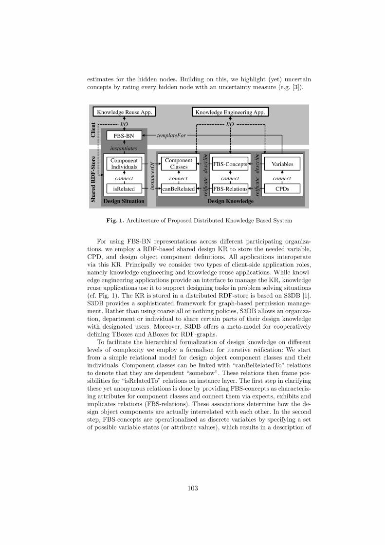
estimates for the hidden nodes. Building on this, we highlight (yet) uncertainconcepts by rating every hidden node with an uncertainty measure (e.g. [3]).

C

lient

Shar

ed R

DF-

Stor

e

Design Situation Design Knowledge

FBS-Relations CPDs

FBS-Concepts Variables

canBeRelated

ComponentClasses

reificate

reificate

describe

describe

connect connect connect

isRelated

ComponentIndividuals

connect

instancesOf

instantiates

templateFor FBS-BN

Knowledge Engineering App.

I/O I/O

Knowledge Reuse App.

Fig. 1. Architecture of Proposed Distributed Knowledge Based System

For using FBS-BN representations across different participating organiza-tions, we employ a RDF-based shared design KR to store the needed variable,CPD, and design object component definitions. All applications interoperatevia this KR. Principally we consider two types of client-side application roles,namely knowledge engineering and knowledge reuse applications. While knowl-edge engineering applications provide an interface to manage the KR, knowledgereuse applications use it to support designing tasks in problem solving situations(cf. Fig. 1). The KR is stored in a distributed RDF-store is based on S3DB [1].S3DB provides a sophisticated framework for graph-based permission manage-ment. Rather than using coarse all or nothing policies, S3DB allows an organiza-tion, department or individual to share certain parts of their design knowledgewith designated users. Moreover, S3DB offers a meta-model for cooperativelydefining TBoxes and ABoxes for RDF-graphs.

To facilitate the hierarchical formalization of design knowledge on differentlevels of complexity we employ a formalism for iterative reification: We startfrom a simple relational model for design object component classes and theirindividuals. Component classes can be linked with “canBeRelatedTo” relationsto denote that they are dependent “somehow”. These relations then frame pos-sibilities for “isRelatedTo” relations on instance layer. The first step in clarifyingthese yet anonymous relations is done by providing FBS-concepts as characteriz-ing attributes for component classes and connect them via expects, exhibits andimplicates relations (FBS-relations). These associations determine how the de-sign object components are actually interrelated with each other. In the secondstep, FBS-concepts are operationalized as discrete variables by specifying a setof possible variable states (or attribute values), which results in a description of

103

the attribute network as configurational variable space. Building on these vari-ables we reificate attribute associations, i.e. we provide a detailed explication ofexpects, exhibits and implicates relations in form of conditional probability ta-bles. Lastly variable and CPD definitions can be used as templates for FBS-BNinstantiation.

3 Conclusion and Future Work

We have outlined a Semantic Web KR of the FBS framework based on RDF,which can be managed in a distributed multi-tenant environment. It is usedto employ FBS-BN-based uncertainty reasoning for lead qualification support.Currently we are implementing two prototype applications, and look forward totest their impact on lead qualification performance empirically.

Acknowledgement This work was partially funded by the German FederalMinistry for Education and Research (BMBF, contract 17N0409). The authorswould like to thank Sabine Janzen, Andreas Filler and Tobias Kowatsch forvaluable discussions.

References

1. Almeida, J.S., Deus, H.F., Maass, W.: S3DB core: a framework for RDF generationand management in bioinformatics infrastructures. BMC Bioinformatics 11(387),pp. 1-10 (2010)

2. Christophe, F.,Bernard, A., Coatanea, E.: RFBS: A model for knowledge represen-tation of conceptual design. CIRP Ann.-Manuf. Techn. 59(1), pp. 155–158 (2010)

3. Eichhoff, J.R., Maass, W.: Representation and Reuse of Design Knowledge: AnApplication for Sales Call Support. In: Konig, A., Dengel, A., Hinkelmann, K.,Kise, K., Howlett, R.J., Jain, L.C. (eds.) KES 2011, Part I. LNAI, vol. 6881, pp.387–396. Springer, Heidelberg (2005)

4. Gero, J.S., Kannengiesser, U.: The situated function-behaviour-structure frame-work. Des. Stud. 25(4), pp. 373–391 (2004)

5. Nikolaidis, E., Mourelatos, Z.P., Pandey, V.: Design Decisions under Uncertaintywith Limited Information. CRC Press/Balkema, Leiden (2011)

6. Szykman, S., Sriram, R.D., Bochenek, C., Racz, J.W., Senfaute, J.: Design Reposito-ries: Next-Generation Engineering Design Databases. IEEE Intell. Syst. App. 15(3),pp. 48–55 (2000)

7. Tuli, K.R., Kohli, A.K., Bharadwaj, S.G.: Rethinking Customer Solutions: FromProduct Bundles to Relational Processes. J. Market. 71(3), pp. 1–17 (2007)

8. Xue, D., Xu, Y.: Web-based distributed system and database modeling for concur-rent design. Computer-Aided Design 35(5), pp. 433–452 (2003)

9. Zhanga, W.Y., Caib, M., Qiuc, J., Yinb, J.W.: Managing distributed manufacturingknowledge through multi-perspective modelling for semantic web applications. Int.J. of Prod. Res. 47(23), pp. 6525–6542 (2009)

10. Zheng, H.-T., B.-Y. Kang, Kim, H.-G.: An ontology-based bayesian network ap-proach for representing uncertainty in clinical practice guidelines. In: Goebel, R.,Siekmann, J., Wahlster, W. (eds.) URSW 2005-2007. LNAI, vol. 5327, pp. 161–173.Springer, Heidelberg (2008)

104

Reasoning under Uncertainty withLog-Linear Description Logics

Mathias Niepert

KR & KM Research Group,Universitat MannheimMannheim, Germany

mathias@informatik.uni-mannheim.de

Abstract. The position paper provides a brief summary of log-lineardescription logics and their applications. We compile a list of five re-quirements that we believe a probabilistic description logic should haveto be useful in practice. We demonstrate the ways in which log-lineardescription logics answer to these requirements.

1 Introduction

Uncertainty is pervasive in the real world and reasoning in its presence one of themost pressing challenges in the development of intelligent systems. It is thereforehard to imagine how the Semantic Web could succeed without the ability torepresent and reason under uncertainty. Nevertheless, purely logical approachesto knowledge representation and reasoning such as description logics have provenuseful in providing the formal backbone of the Semantic Web. There is not onlya large body of important work on the logical and algorithmic properties ofsuch languages but also highly optimized tools that are successfully employedin meaningful applications. Still, the need to model uncertainty persists. Twoprominent examples where the processing of uncertainty is crucial are (a) dataintegration (schema and instance alignment) and (b) ontology learning. In bothcases, algorithms usually generate confidence values for particular axioms. Inontology matching, for instance, string similarity measures are often used tofind confidence values for equivalence axioms between concepts and properties,respectively.

There have been attempts to combine logic and probability in various ways.Resulting approaches are probabilistic formalism for description logics [4, 5, 2,6, 8] and, more generally, statistical relational languages [3]. The former areimportant theoretical contributions but have not been adopted by practitioners.We believe this is primarily due to the computational complexity of probabilisticinference, the rather involved way of expressing uncertainties syntactically, andthe lack of implementations. Statistical relational approaches, on the other hand,have been successfully applied to numerous real-world problems but they do notexplicitly take into account the notion of coherency and consistency which iscrucial in the context of the Semantic Web.

105

Name Syntax Semantics

top > ∆I

bottom ⊥ ∅nominal a aI

conjunction C uD CI ∩DI

existential restriction ∃r.C x ∈ ∆I |∃y ∈ ∆I : (x, y) ∈ rI ∧ y ∈ CIGCI C v D CI ⊆ DI

RI r1 ... rk v r rI1 ... rIk ⊆ rITable 1. The description logic EL++ without nominals and concrete domains.

Based on these observations (and biases), and with the more concrete ap-plications of ontology learning and matching in mind, we have compiled thefollowing wish list for a probabilistic description logic.

1. The system must be usable by individuals knowledgeable only in SemanticWeb languages and tools such as OWL and Protege;

2. It must be possible to express uncertainty in form of degrees of confidence(real-valued weights) and not necessarily in form of precise probabilities.Real-world problems such as ontology matching and learning require this;

3. The user should not have to worry about inconsistent and incoherent inputto the probabilistic reasoner. All types of inconsistencies are handled by theprobabilistic reasoner and not the user;

4. Two types of queries should be supported under uncertainty: (a) The “mostprobable ontology” query and (b) the probability of (conjunctions) of axiomsquery; and

5. The worst-case complexity should not exceed that of probabilistic graphicalmodels such as Markov and Bayesian networks. While inference in thesemodels is generally NP-hard, numerous highly efficient algorithms exist andcan be employed in the context of probabilistic DLs.

These five requirements are captured by log-linear description logics [7]. Weprovide a brief overview of log-linear description logics and discuss how thisfamily of probabilistic logics answers to the outlined requirements.

2 Log-Linear Description Logics

Log-linear description logics integrate description logics with probabilistic log-linear models. Detailed technical and empirical results are available [7] and aremostly omitted in this position paper. The syntax of log-linear description logicsis taken from the underlying description logic. However, it is possible to assignreal-valued weights to axioms. Here, we focus on the log-linear description logicbased on EL++ [1] without concrete domains (see Table 1) which we denote as

106

EL++-LL. EL++ captures the expressivity of numerous ontologies in the biomed-ical sciences and other domains, and it is the description logic on which the webontology language profile OWL 2 EL is based. More formally, a EL++-LL on-tology C = (CD, CU) is a pair consisting of a deterministic EL++ CBox (set ofaxioms) CD and an uncertain CBox CU = (c, wc) which is a set of pairs (c, wc)with each c being a EL++ axiom and w a real-valued weight assigned to c. Whilethe deterministic CBox contains axioms that are known to be true the uncer-tain CBox contains axioms for which we only have a degree of confidence. Everyaxiom can either be part of the deterministic or the uncertain CBox but not ofboth.

The semantics of log-linear DLs is based on joint probability distributionsover coherent EL++ CBoxes and similar to that of Markov logic [9]. The weightsof the axioms determine the log-linear probability distribution. For a EL++-LL CBox (CD, CU) and a EL++ CBox C′ over the same set of basic conceptdescriptions and role names, we have that

P (C′) =

1Z exp

(∑(c,wc)∈CU:C′|=c wc

) if C′ is coherentand C′ |= CD;

0 otherwise

where Z is the normalization constant of the log-linear probability distribution.The semantics of the log-linear description logic leads to probability distri-

butions one would expect under the open world semantics of description logics.

Example 1. Let Student and Professor be two classes and let CD = ∅ and CU =〈Student v Professor, 0.5〉, 〈StudentuProfessor v⊥, 0.5〉. Then1, P (Student vProfessor, StudentuProfessor v⊥) = 0, P (Student v Professor) = Z−1 exp(0.5),P (Student v Professor, Professor v Student) = Z−1 exp(0.5), P (Student uProfessor v⊥) = Z−1 exp(0.5), P (Professor v Student) = Z−1 exp(0), andP (∅) = Z−1 exp(0) with Z = 3 exp(0.5) + 2 exp(0).

We distinguish two types of probabilistic queries. The maximum a-posteriori(MAP) query: “Given a EL++-LL CBox, what is a most probable coherent EL++

CBox over the same concept and role names?”; and the conditional probabilityquery: “Given a EL++-LL CBox, what is the probability of a conjunction of ax-ioms?” We believe that the first type of query is useful since it infers the mostprobable coherent ontology from one that contains axioms with confidence val-ues. The MAP query, therefore, has immediate applications in ontology learningand matching.

Probabilistic inference in log-linear description logics seems daunting at first,considering the combinatorial complexity of the problem. It turns out, however,that both the MAP and the conditional probability query can be computedefficiently for ontologies with thousands of known and uncertain axioms [7]. Theworst-case complexity of both queries is equivalent to the worst-case complexityof the analogous queries in Markov and Bayesian networks (requirement 5).1 We omit trivial axioms that are present in every classified CBox such as Student v >

and Student v Student.

107

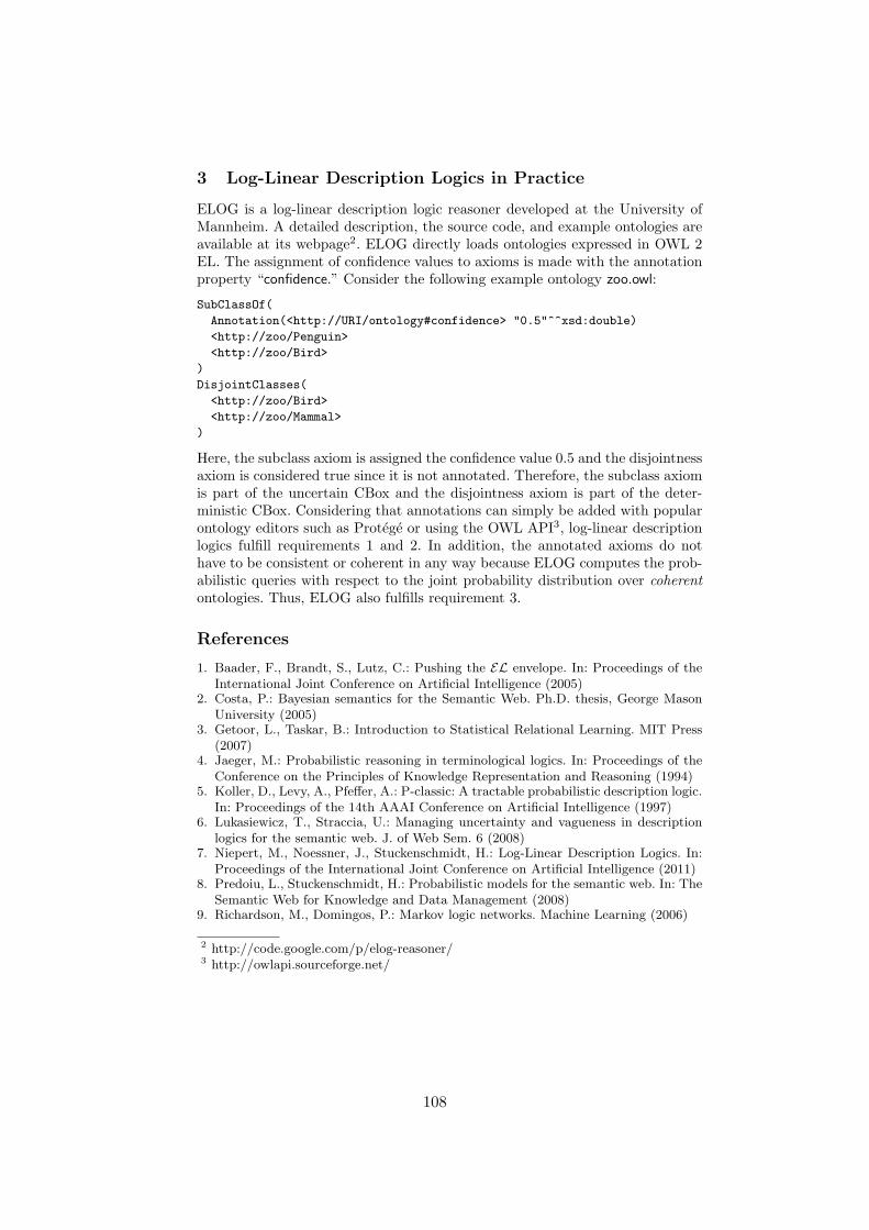
3 Log-Linear Description Logics in Practice

ELOG is a log-linear description logic reasoner developed at the University ofMannheim. A detailed description, the source code, and example ontologies areavailable at its webpage2. ELOG directly loads ontologies expressed in OWL 2EL. The assignment of confidence values to axioms is made with the annotationproperty “confidence.” Consider the following example ontology zoo.owl:

SubClassOf(

Annotation(<http://URI/ontology#confidence> "0.5"^^xsd:double)

<http://zoo/Penguin>

<http://zoo/Bird>

)

DisjointClasses(

<http://zoo/Bird>

<http://zoo/Mammal>

)

Here, the subclass axiom is assigned the confidence value 0.5 and the disjointnessaxiom is considered true since it is not annotated. Therefore, the subclass axiomis part of the uncertain CBox and the disjointness axiom is part of the deter-ministic CBox. Considering that annotations can simply be added with popularontology editors such as Protege or using the OWL API3, log-linear descriptionlogics fulfill requirements 1 and 2. In addition, the annotated axioms do nothave to be consistent or coherent in any way because ELOG computes the prob-abilistic queries with respect to the joint probability distribution over coherentontologies. Thus, ELOG also fulfills requirement 3.

References

1. Baader, F., Brandt, S., Lutz, C.: Pushing the EL envelope. In: Proceedings of theInternational Joint Conference on Artificial Intelligence (2005)

2. Costa, P.: Bayesian semantics for the Semantic Web. Ph.D. thesis, George MasonUniversity (2005)

3. Getoor, L., Taskar, B.: Introduction to Statistical Relational Learning. MIT Press(2007)

4. Jaeger, M.: Probabilistic reasoning in terminological logics. In: Proceedings of theConference on the Principles of Knowledge Representation and Reasoning (1994)

5. Koller, D., Levy, A., Pfeffer, A.: P-classic: A tractable probabilistic description logic.In: Proceedings of the 14th AAAI Conference on Artificial Intelligence (1997)

6. Lukasiewicz, T., Straccia, U.: Managing uncertainty and vagueness in descriptionlogics for the semantic web. J. of Web Sem. 6 (2008)

7. Niepert, M., Noessner, J., Stuckenschmidt, H.: Log-Linear Description Logics. In:Proceedings of the International Joint Conference on Artificial Intelligence (2011)

8. Predoiu, L., Stuckenschmidt, H.: Probabilistic models for the semantic web. In: TheSemantic Web for Knowledge and Data Management (2008)

9. Richardson, M., Domingos, P.: Markov logic networks. Machine Learning (2006)

2 http://code.google.com/p/elog-reasoner/3 http://owlapi.sourceforge.net/

108

Handling uncertainty in information extraction

Maurice van Keulen1 and Mena B. Habib1

University of Twente, Faculty of EEMCS, Enschede, The Netherlandsm.vankeulen,m.badiehhabibmorgan@utwente.nl

Abstract. This position paper proposes an interactive approach for de-veloping information extractors based on the ontology definition processwith knowledge about possible (in)correctness of annotations. We discussthe problem of managing and manipulating probabilistic dependencies.

1 Introduction

(Too) much data is still inaccessible for data processing, because it is unstruc-tured, textually embedded in documents, webpages, or text fields in databases.Information extraction (IE) is a technology capable of extracting entities, facts,and relations. IE helps to turn the web into a real ‘web of data’ [BHBL09].

In the Neogeography-project [HvK11b], we focus on named entity extraction(NEE) from database text fields and short messages. NEE typically consists ofphases like recognition (which phrases are named entities), matching and enrich-ment (lookups in reference databases and dictionaries possibly adding informa-tion), and disambiguation (to which real-world object does a phrase refer).

Because natural language is highly ambiguous and computers are still inca-pable of ‘real’ semantic understanding, NEE (and IE in general) is a highly im-perfect process. For example, it is ambiguous how to interpret the word “Paris”:it could be a first name, a city, etc. Even resolving it to a city, a lookup inGeoNames1 learns that there are numerous other places called “Paris” besidesthe capital of France. In [HvK11a], we found that around 46% of toponyms2 havetwo or more, 35% three or more, and 29% four or more references in GeoNames.

Although many probabilistic and fuzzy techniques abound, some aspects of-ten remain absolute: extraction rules absolutely recognize and annotate a phraseor not, only a top item from a ranking is chosen for a next phase, etc. We envisionan approach that fundamentally treats annotations and extracted informationas uncertain throughout the process. We humans happily deal with doubt andmisinterpretation every day, why shouldn’t computers?

We envision developing information extractors ‘Sherlock Holmes style’ —“when you have eliminated the impossible, whatever remains, however improba-ble, must be the truth” — by adopting the principles and requirements below.– Annotations are uncertain, hence we process both annotations as well as

information about the uncertainty surrounding them.1 http://www.geonames.org2 A toponym is any name that refers to a location including, e.g., names of buildings.

109

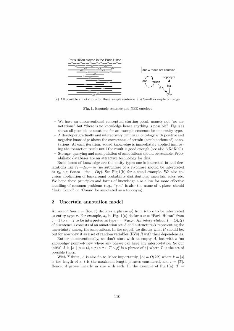
Paris Hilton stayed in the Paris Hiltona1 a2 a3 a4 a5 a6 a7

a8 a9 a10a11 a12a12 a13

a14 a15a16 a17

a18a19

a20a21

a22a23

a24a25

a26a27

a28

(a) All possible annotations for the example sentence

PersonToponym

City

dnc

dnc isa

dnc = "does not contain"

(b) Small example ontology

Fig. 1. Example sentence and NEE ontology

– We have an unconventional conceptual starting point, namely not “no an-notations” but “there is no knowledge hence anything is possible”. Fig.1(a)shows all possible annotations for an example sentence for one entity type.

– A developer gradually and interactively defines an ontology with positive andnegative knowledge about the correctness of certain (combinations of) anno-tations. At each iteration, added knowledge is immediately applied improv-ing the extraction result until the result is good enough (see also [vKdK09]).

– Storage, querying and manipulation of annotations should be scalable. Prob-abilistic databases are an attractive technology for this.Basic forms of knowledge are the entity types one is interested in and dec-

larations like τ1 —dnc— τ2 (no subphrase of a τ1-phrase should be interpretedas τ2, e.g, Person —dnc— City). See Fig.1(b) for a small example. We also en-vision application of background probability distributions, uncertain rules, etc.We hope these principles and forms of knowledge also allow for more effectivehandling of common problems (e.g., “you” is also the name of a place; should“Lake Como” or “Como” be annotated as a toponym).

2 Uncertain annotation model

An annotation a = (b, e, τ) declares a phrase ϕbe from b to e to be interpreted

as entity type τ . For example, a8 in Fig. 1(a) declares ϕ = “Paris Hilton” fromb = 1 to e = 2 to be interpreted as type τ = Person. An interpretation I = (A,U)of a sentence s consists of an annotation set A and a structure U representing theuncertainty among the annotations. In the sequel, we discuss what U should be,but for now view it as a set of random variables (RVs) R with their dependencies.

Rather unconventionally, we don’t start with an empty A, but with a ‘noknowledge’ point-of-view where any phrase can have any interpretation. So ourinitial A is a | a = (b, e, τ) ∧ τ ∈ T ∧ ϕb

e is a phrase of s where T is the set ofpossible types.

With T finite, A is also finite. More importantly, |A| = O(klt) where k = |s|is the length of s, l is the maximum length phrases considered, and t = |T |.Hence, A grows linearly in size with each. In the example of Fig.1(a), T =

110

∅

a∧b

a∧¬b

b∧¬a

0.48

0.12

0.32

0.08

(a) Annotations a and b independent withprobabilities P (a) = 0.6 and P (b) = 0.8

∅ a∧¬b

b∧¬a

0.23

0.62

0.15

(b) a and b conditioned to be mutuallyexclusive (a ∧ b not possible)

Fig. 3. Defining a and b to be mutually exclusive means conditioning the probabilities.

Person, Toponym, City and we have 28 · |T | = 84 annotations. Even though weenvision a more ingenious implementation, no probabilistic database would beseverely challenged by a complete annotation set for a typical text field.

3 Knowledge application is conditioning

We explain how to ‘apply knowledge’ in our approach by means of the exampleof Fig.1, i.e., with our A with 84 (possible) annotations and an ontology onlycontaining Person, Toponym, and City. Suppose we like to add the knowledgePerson —dnc— City. The effect should be the removal of some annotations andadjustment of the probabilities of the remaining ones.

annotationsb e type . . . wsd

a11 1 1 Person . . . x1

1 = 1a21 1 1 City . . . x2

1 = 1a18 1 2 Person . . . x1

8 = 1. . . . . . . . . . . .

world setx v P

x11 0 0.4

x11 1 0.6

x21 0 0.7

x21 1 0.3

x18 0 0.2

x18 1 0.8

. . . . . . . . .

Fig. 2. Initial annotation set stored in aprobabilistic database (MayBMS-style)

An initial promising idea is to storethe annotations in an uncertain rela-tion in a probabilistic database, suchas MayBMS [HAKO09]. In MayBMS,the existence of each tuple is deter-mined by an associated world set de-scriptor (wsd) containing a set of RVassignments from a world set table (seeFig.2). RVs are assumed independent.For example, the 3rd annotation tupleonly exists when x1

8 = 1 which is the case with a probability of 0.8. Each an-notation can be seen as a probabilistic event, which are all independent in ourstarting point. Hence, we can store A by associating each annotation tuple aj

i

with one boolean RV xji . Consequently, the database size is linear with |A|.

Adding knowledge such as Person—dnc—City means that certain RVs becomedependent and that certain combinations of RV assignments become impossible.Let us focus on two individual annotations a2

1 (’“Paris” is a City) and a18 (“Paris

Hilton” is a Person). These two annotations become mutually exclusive. Theprocess of adjusting the probabilities is called conditioning [KO08]. It boils downto redistributing the remaining probability mass. Fig.3 illustrates this for a = a2

1

and b = a18. The remaining probability mass is 1 − 0.48 = 0.52. Hence, the

111

distribution of this mass over the remaining possibilities is P (a ∧ ¬b) = 0.120.52 ≈

0.23, P (b ∧ ¬a) = 0.320.52 ≈ 0.62, and P (∅) = P (¬a ∧ ¬b) = 0.08

0.52 ≈ 0.15.

A first attempt is to replace x21 and x1

8 with one fresh three-valued RV x′ withthe probabilities just calculated, i.e., wsd(a2

1) = x′ = 1 and wsd(a18) = x′ = 2

with P (x′ = 0) = 0.15, P (x′ = 1) = 0.23, and P (x′ = 2) = 0.62. Unfortunately,since annotations massively overlap, we face a combinatorial explosion. For thisrule, we end up with one RV with up to 22·28 = 256 ≈ 7 · 1016 cases.

Solution directions What we are looking for in this paper is a structure that isexpressive enough to capture all dependencies between RVs and at the same timeallowing for scalable processing of conditioning operations. The work of [KO08]represents dependencies resulting from queries with a tree of RV assignments.We are also investigating the shared correlations work of [SDG08].

4 Conclusions

We envision an approach where information extractors are developed based onan ontology definition process for knowledge about possible (in)correctness ofannotations. Main properties are treating annotations as fundamentally uncer-tain and interactive addition of knowledge starting from a ‘no knowledge henceeverything is possible’ situation. The feasibility of the approach hinges on effi-cient storage and conditioning of probabilistic dependencies. We discuss this veryproblem, argue that a trivial approach doesn’t work, and propose two solutiondirections: the conditioning approach of MayBMS and the shared correlationswork of Getoor et al.

References

[BHBL09] C. Bizer, T. Heath, and T. Berners-Lee. Linked data: The story so far. Int’lJ. on Semantic Web and Information Systems (IJSWIS), 5(3):1–22, 2009.

[HAKO09] J. Huang, L. Antova, C. Koch, and D. Olteanu. MayBMS: a probabilisticdatabase management system. In Proc. of the 35th SIGMOD Int’l Conf. onManagement Of Data, Providence, Rhode Island, pages 1071–1074, 2009.

[HvK11a] M. B. Habib and M. van Keulen. Named entity extraction and disam-biguation: The reinforcement effect. In Proc. of the 5th Int’l Workshop onManagement of Uncertain Data (MUD), Seatle, 29 Aug, pages 9–16, 2011.

[HvK11b] M. B. Habib and M. van Keulen. Neogeography: The challenge of chan-nelling large and ill-behaved data streams. Technical Report TR-CTIT-11-08, Enschede, 2011. ISSN 1381-3625, http://eprints.eemcs.utwente.nl/19854.

[KO08] C. Koch and D. Olteanu. Conditioning probabilistic databases. Proc. VLDBEndow., 1(1):313–325, 2008.

[SDG08] P. Sen, A. Deshpande, and L. Getoor. Exploiting shared correlations inprobabilistic databases. Proc. VLDB Endow., 1(1):809–820, 2008.

[vKdK09] M. van Keulen and A. de Keijzer. Qualitative effects of knowledge rulesand user feedback in probabilistic data integration. The VLDB Journal,18(5):1191–1217, 2009.

112