702341 QA in Finance/ Ch 3 Probability in Finance Probability.
49
702341 QA in Finance/ Ch 3 Probability in Finance Probability
-
Upload
stuart-davis -
Category
Documents
-
view
232 -
download
1
Transcript of 702341 QA in Finance/ Ch 3 Probability in Finance Probability.

702341 QA in Finance/ Ch 3 Probability in Finance
Probability

702341 QA in Finance/ Ch 3 Probability in Finance
Probability
Probability is a measure of the possibility of an event happening
Measure on a scale between zero and one Probability has a substantial role to play in financial
analysis as the outcomes of financial decisions are uncertain
e.g. Fluctuation in share prices

702341 QA in Finance/ Ch 3 Probability in Finance
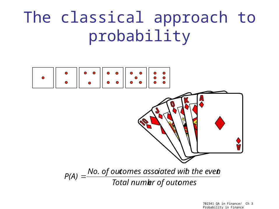
The classical approach to probability
The range of possible uncertain outcomes is known and equally likely
EXPERIMENT, SAMPLE, EVENT
consider the tossing of a fair coin:
the range is limited to two
the tossing of the coin is the experiment
the two possible outcomes refer to the sample space
the outcome whether it is head or tail is the event
702341 QA in Finance/ Ch 3 Probability in Finance
The classical approach to probability
omeser of outcTotal numb
th the evenciated witcomes assoNo. of outP(A)
702341 QA in Finance/ Ch 3 Probability in Finance
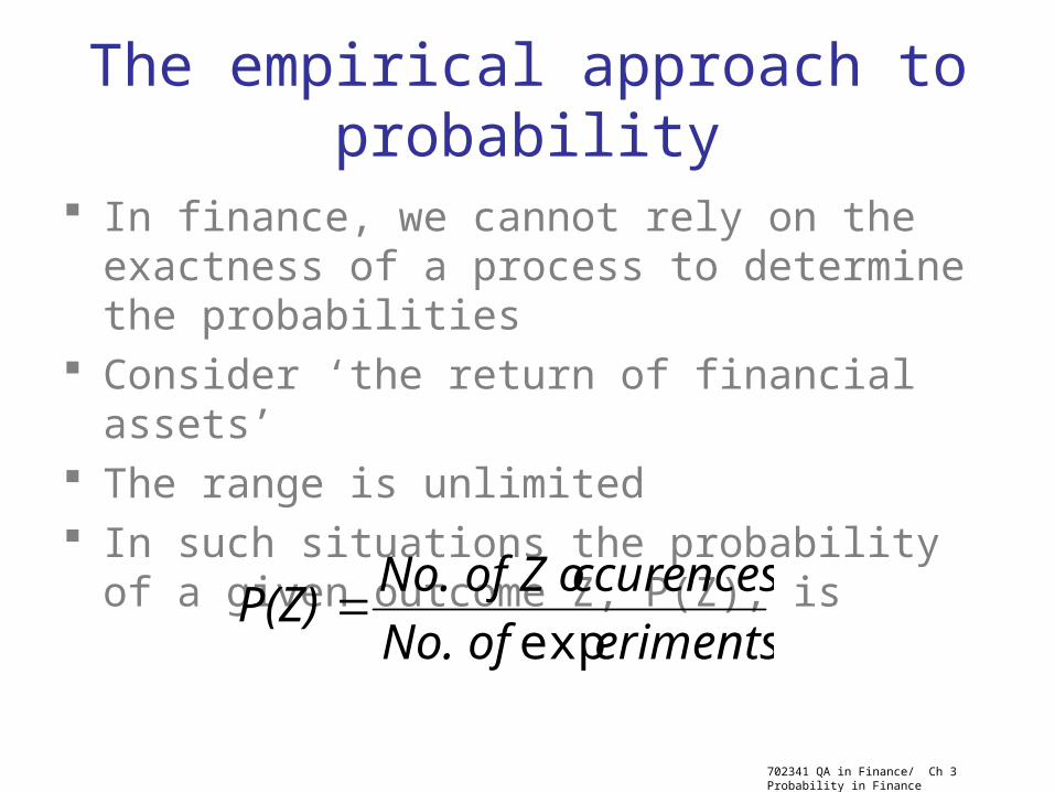
The empirical approach to probability
In finance, we cannot rely on the exactness of a process to determine the probabilities
Consider ‘the return of financial assets’ The range is unlimited In such situations the probability of a given outcome
Z, P(Z), is
erimentsNo. of
ccurencesNo. of Z oP(Z)
exp

702341 QA in Finance/ Ch 3 Probability in Finance
The empirical approach to probability
E.g. Consider a sample of 100 daily movements in a share price. Assume that of the 100 absolute movements, five movements were 0.5 Baht each, 15 were 1 Baht each, 20 were 1.5 Baht each, 30 were 2 Baht each, 20 were 2.5 Baht and 10 were 3 Baht each

702341 QA in Finance/ Ch 3 Probability in Finance
Basic rules of probability
These rules are : the addition rule concerned with A or B happening the multiplication rule concerned with A and B occurring
Which of these rules is applicable will depend on whether the combined events are INDEPENDENT or MUTUALLY EXCLUSIVE ???

702341 QA in Finance/ Ch 3 Probability in Finance
Mutually exclusive
Two events cannot occur together
Sample space = {1,2,3,4,5,6}
A is the event that the face of die shows odd number:
A = {1,3,5}
B is the event that the face of die is even number:
B = {2,4,6}
A Λ B = { } = Ø
A and B is MUTUALLY EXCLUSIVE

702341 QA in Finance/ Ch 3 Probability in Finance
Mutually exclusive
A B

702341 QA in Finance/ Ch 3 Probability in Finance
The addition rule applied to non-mutually exclusive events
P(A or B) = P(A) + P(B) – P(A and B)
Assume that the FTSE 100 index may rise with a probability of 0.55 and fall with the probability of 0.45. Also assume that a particular time interval the S&P index may rise with a probability of 0.35 and fall with a probability of 0.65. There is also a probability of 0.3 that both indices rise together. What is the probability of wither the FTSE 100 index or the S&P 500 index rising
A B
702341 QA in Finance/ Ch 3 Probability in Finance
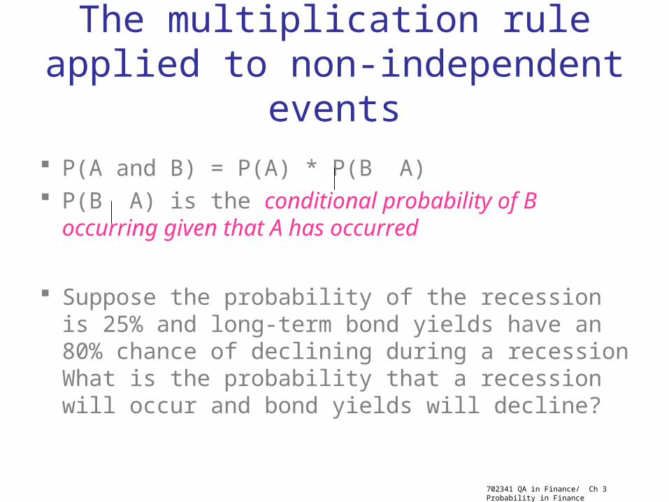
The multiplication rule applied to non-independent events
P(A and B) = P(A) * P(B A) P(B A) is the conditional probability of B occurring
given that A has occurred
Suppose the probability of the recession is 25% and long-term bond yields have an 80% chance of declining during a recession What is the probability that a recession will occur and bond yields will decline?

702341 QA in Finance/ Ch 3 Probability in Finance
Bayes’ theorem
Manipulation of the general multiplication rule The probability of the updated event An can be
updated to P(A|B) if Scenario B is known to have occurred by using the following relationships
Ni
iii
kkk
ABPAP
ABPAPBAP
1
))/().((
)/().()/(
702341 QA in Finance/ Ch 3 Probability in Finance
Bayes’ theorem
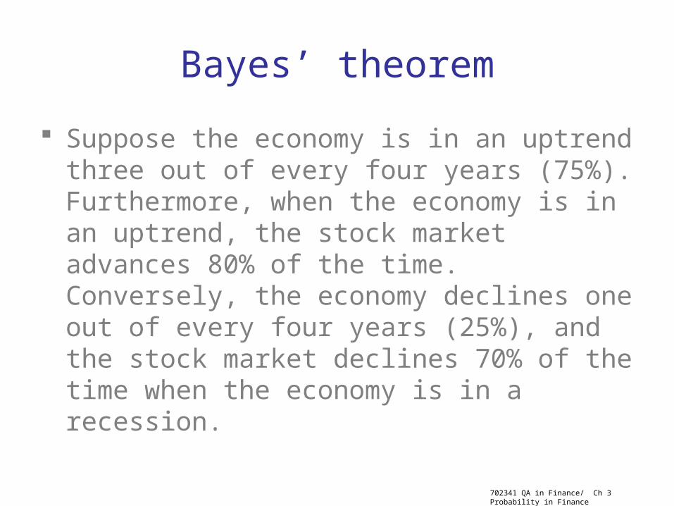
Suppose the economy is in an uptrend three out of every four years (75%). Furthermore, when the economy is in an uptrend, the stock market advances 80% of the time. Conversely, the economy declines one out of every four years (25%), and the stock market declines 70% of the time when the economy is in a recession.
702341 QA in Finance/ Ch 3 Probability in Finance
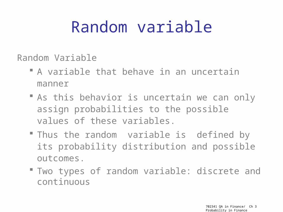
Random variable
Random Variable
A variable that behave in an uncertain manner
As this behavior is uncertain we can only assign probabilities to the possible values of these variables.
Thus the random variable is defined by its probability distribution and possible outcomes.
Two types of random variable: discrete and continuous
702341 QA in Finance/ Ch 3 Probability in Finance
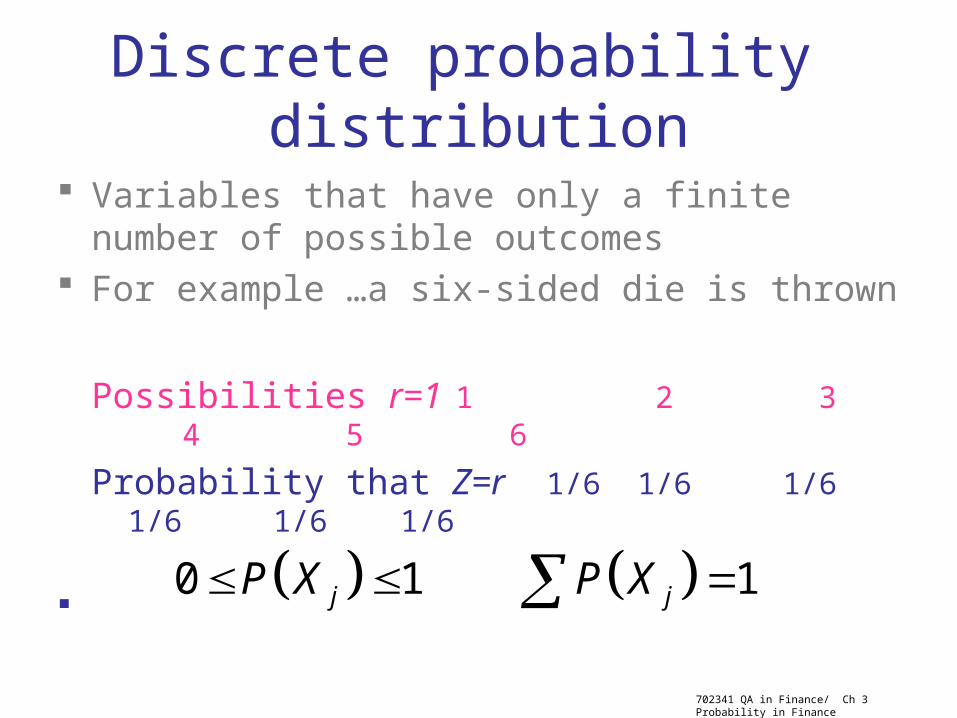
Discrete probability distribution
Variables that have only a finite number of possible outcomes
For example …a six-sided die is thrown
Possibilities r=1 1 2 3 4 5 6
Probability that Z=r 1/6 1/6 1/6 1/6 1/6 1/6
0 1 1j jP X P X
702341 QA in Finance/ Ch 3 Probability in Finance
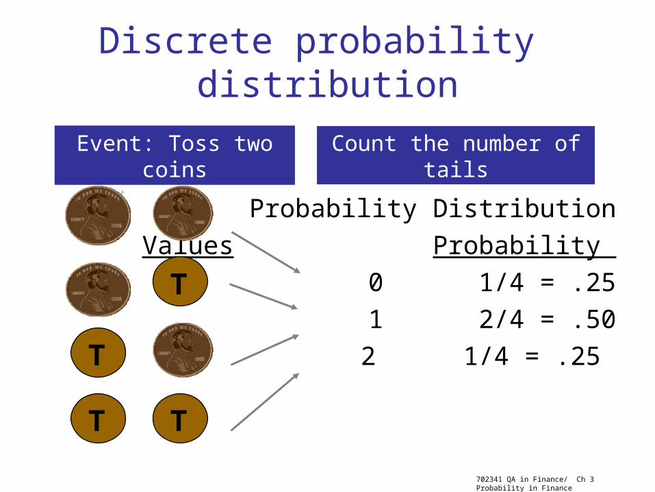
Discrete probability distribution
Probability Distribution
Values Probability
0 1/4 = .25
1 2/4 = .50
2 1/4 = .25
Event: Toss two coins Count the number of tails
T
T
T T

702341 QA in Finance/ Ch 3 Probability in Finance
Continuous probability distribution
Variables that can be subdivided into an infinite number of subunits for measurement
For example …speed, asset returns Consider: a movement in an asset price from 105 to
109 will give a return of … %

702341 QA in Finance/ Ch 3 Probability in Finance
Continuous probability distribution
To overcome this practical problem, we must define our continuous random variable by integrating what is know as a probability density function (pdf)
1)( dXXf
702341 QA in Finance/ Ch 3 Probability in Finance
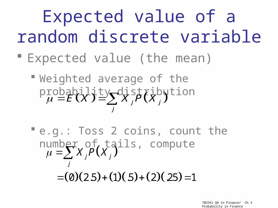
Expected value of a random discrete variable
Expected value (the mean)
Weighted average of the probability distribution
e.g.: Toss 2 coins, count the number of tails, compute
j jj
E X X P X
0 2.5 1 .5 2 .25 1
j jj
X P X
702341 QA in Finance/ Ch 3 Probability in Finance
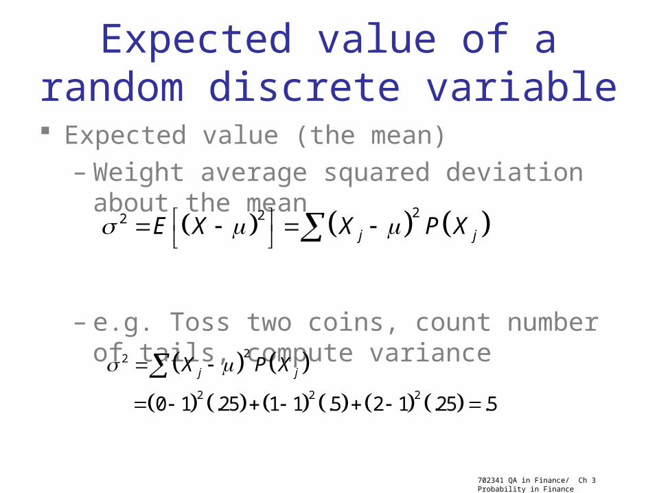
Expected value of a random discrete variable
Expected value (the mean)– Weight average squared deviation about the mean
– e.g. Toss two coins, count number of tails, compute variance
222j jE X X P X
22
2 2 2 0 1 .25 1 1 .5 2 1 .25 .5
j jX P X

702341 QA in Finance/ Ch 3 Probability in Finance
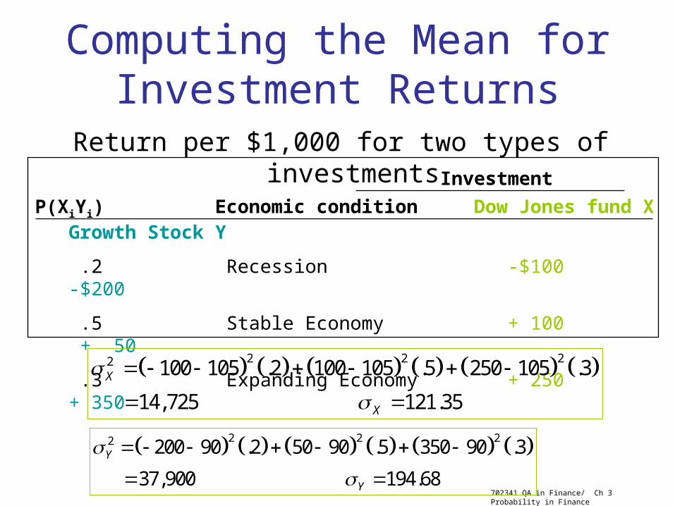
Computing the Mean for Investment Returns
Return per $1,000 for two types of investments
P(XiYi) Economic condition Dow Jones fund X Growth Stock Y
.2 Recession -$100 -$200
.5 Stable Economy + 100 + 50
.3 Expanding Economy + 250 + 350
Investment
100 .2 100 .5 250 .3 $105XE X
200 .2 50 .5 350 .3 $90YE Y
702341 QA in Finance/ Ch 3 Probability in Finance
Computing the Mean for Investment Returns
Return per $1,000 for two types of investments
P(XiYi) Economic condition Dow Jones fund X Growth Stock Y
.2 Recession -$100 -$200
.5 Stable Economy + 100 + 50
.3 Expanding Economy + 250 + 350
Investment
2 2 22 100 105 .2 100 105 .5 250 105 .3
14,725 121.35X
X
2 2 22 200 90 .2 50 90 .5 350 90 .3
37,900 194.68Y
Y

702341 QA in Finance/ Ch 3 Probability in Finance
Probability Distribution
Important probability distributions in finance
Discrete: BINOMIAL POISSON
Continuous: NORMAL LOG NORMAL
702341 QA in Finance/ Ch 3 Probability in Finance
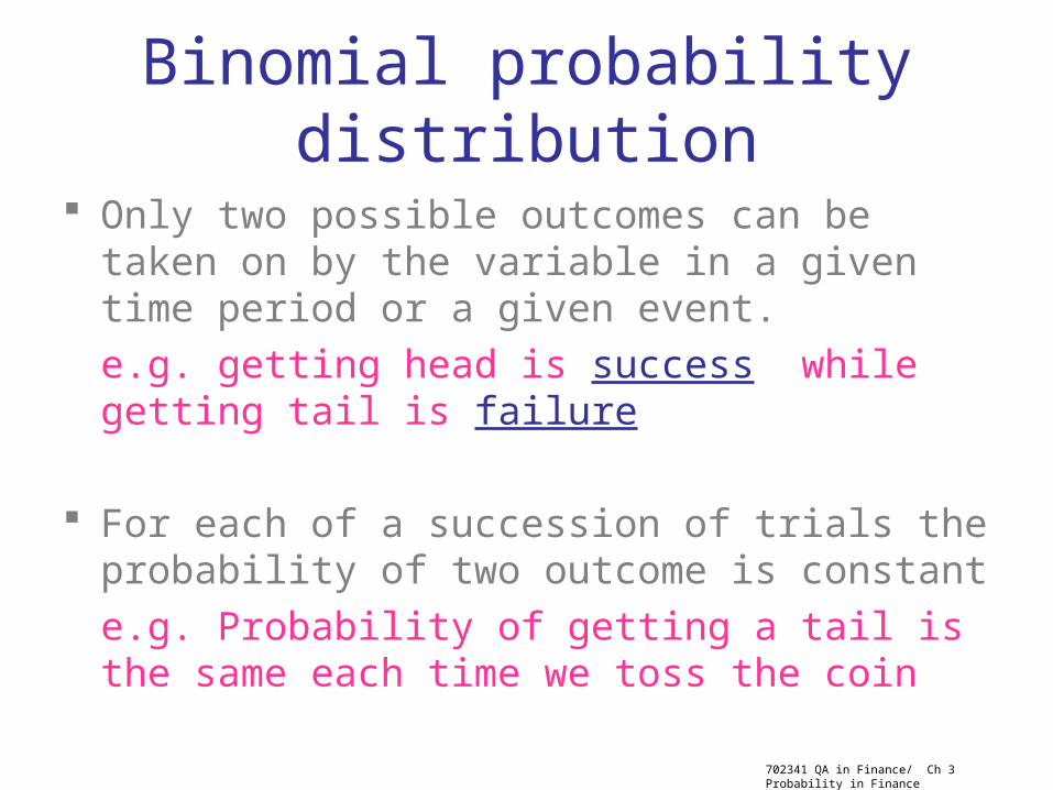
Binomial probability distribution
Only two possible outcomes can be taken on by the variable in a given time period or a given event.
e.g. getting head is success while getting tail is failure
For each of a succession of trials the probability of two outcome is constant
e.g. Probability of getting a tail is the same each time we toss the coin
702341 QA in Finance/ Ch 3 Probability in Finance
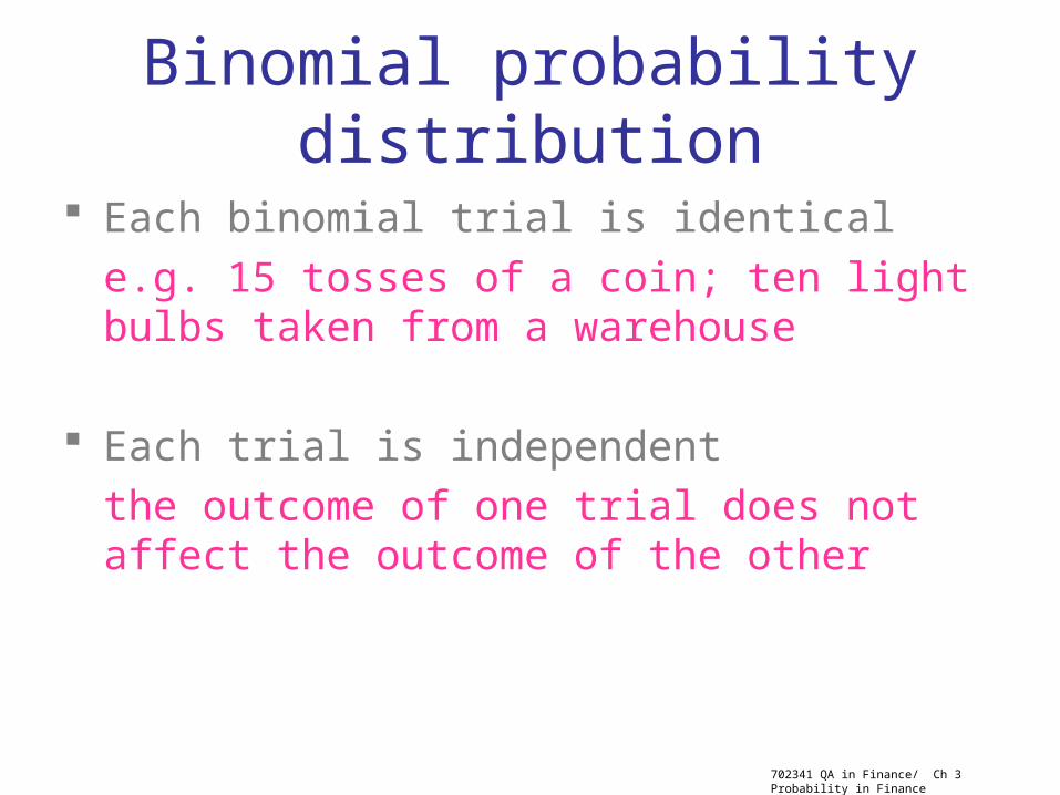
Binomial probability distribution
Each binomial trial is identical
e.g. 15 tosses of a coin; ten light bulbs taken from a warehouse
Each trial is independent
the outcome of one trial does not affect the outcome of the other
702341 QA in Finance/ Ch 3 Probability in Finance
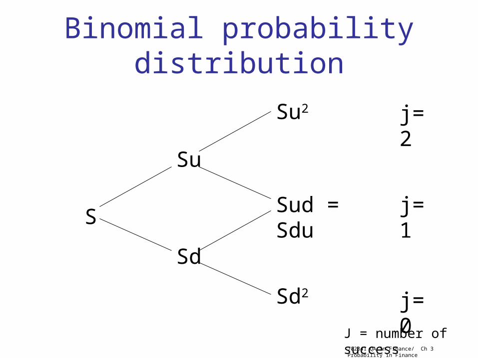
Binomial probability distribution
Sd
Su
S
Su2
Sud = Sdu
Sd2
j=2
j=1
j=0
J = number of success
702341 QA in Finance/ Ch 3 Probability in Finance
Binomial probability distribution
The probability of achieving each outcome depends on:
1. the probability of achieving a success
2. the total number of ways of achieving that outcome
e.g. consider the case of j = 1 (Sdu = Sud)
1. each way has a probability of 0.25
2. there are two ways to achieving an outcome

702341 QA in Finance/ Ch 3 Probability in Finance
Binomial probability distribution
!1
! !
: probability of successes given and
: number of "successes" in sample 0,1, ,
: the probability of each "success"
: sample size
n XXnP X p p
X n X
P X X n p
X X n
p
n
Combination rule
or the number of binomial trials
702341 QA in Finance/ Ch 3 Probability in Finance
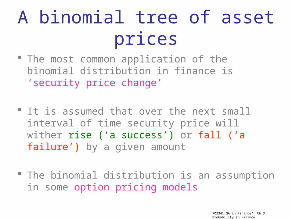
A binomial tree of asset prices
The most common application of the binomial distribution in finance is ‘security price change’
It is assumed that over the next small interval of time security price will wither rise (‘a success’) or fall (‘a failure’) by a given amount
The binomial distribution is an assumption in some option pricing models

702341 QA in Finance/ Ch 3 Probability in Finance
A binomial tree of asset prices
3 stages in developing the expected value of asset price: create a binomial lattice determine the probabilities of each outcome multiply each possible outcome by the appropriate
probability and sum the products to arrive at the expected value
702341 QA in Finance/ Ch 3 Probability in Finance
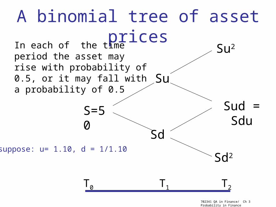
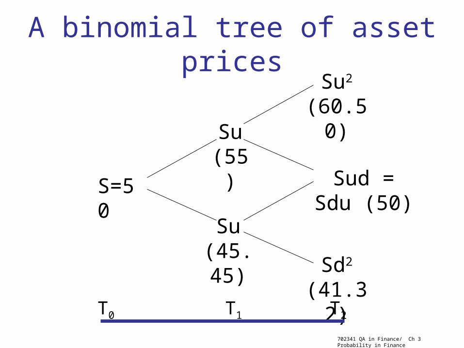
A binomial tree of asset prices
Sd
Su
S=50
Su2
Sud = Sdu
Sd2
T0 T1 T2
In each of the time period the asset may rise with probability of 0.5, or it may fall with a probability of 0.5
suppose: u= 1.10, d = 1/1.10
702341 QA in Finance/ Ch 3 Probability in Finance
A binomial tree of asset prices
Su (45.45)
Su (55)
S=50
Su2
(60.50)
Sud = Sdu (50)
Sd2
(41.32)T0 T1 T2

702341 QA in Finance/ Ch 3 Probability in Finance
A binomial tree of asset prices
The expected value is calculated as:
(60.50 x 0.25) + (50.0 x 0.50) + (41.32 x 0.25)
= 50.46
The variance is
(60.50-50.46)2 x 0.25 + (50.0-50.46)2 x 0.50 + (41.32-50.46)2 x 0.25
= 46.18
702341 QA in Finance/ Ch 3 Probability in Finance
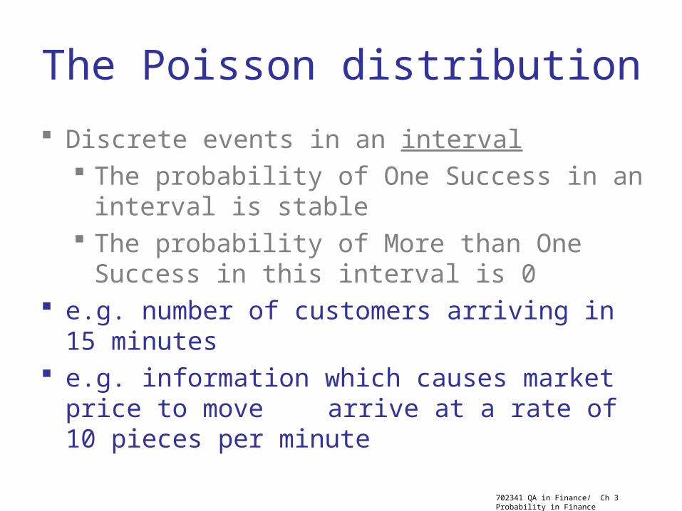
The Poisson distribution
Discrete events in an interval The probability of One Success in an interval is
stable The probability of More than One Success in this
interval is 0 e.g. number of customers arriving in 15 minutes e.g. information which causes market price to move
arrive at a rate of 10 pieces per minute

702341 QA in Finance/ Ch 3 Probability in Finance
The Poisson distribution
!
: probability of "successes" given
: number of "successes" per unit
: expected (average) number of "successes"
: 2.71828 (base of natural logs)
XeP X
XP X X
X
e

702341 QA in Finance/ Ch 3 Probability in Finance
The Poisson distribution
ex. Find the probability of 4 customers arriving in 3 minutes when the mean is 3.6.
ex. information which causes market price to move arrive at a rate of 10 pieces per minute. Find the
probability of only eight pieces of information arriving in the next minute ???
3.6 43.6
.19124!
eP X
702341 QA in Finance/ Ch 3 Probability in Finance
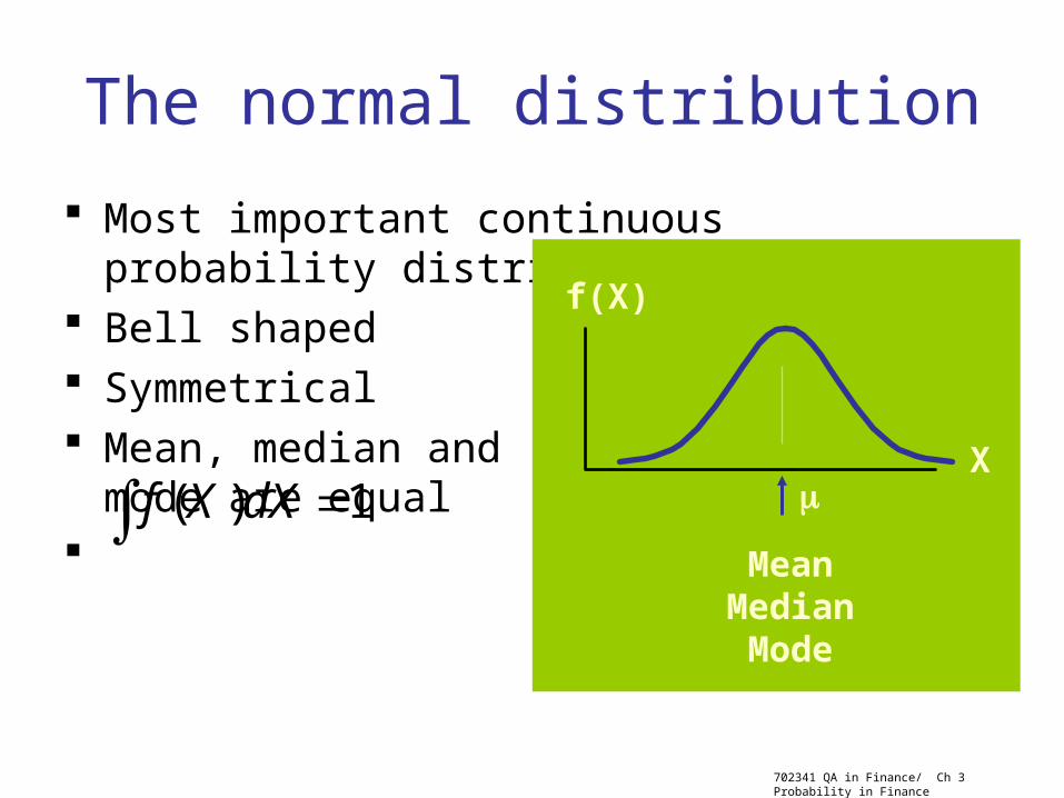
The normal distribution
Most important continuous probability distribution Bell shaped Symmetrical Mean, median and
mode are equal
Mean Median Mode
X
f(X)
1)( dXXf

702341 QA in Finance/ Ch 3 Probability in Finance
The normal distribution
21
2
2
1
2
: density of random variable
3.14159; 2.71828
: population mean
: population standard deviation
: value of random variable
X
f X e
f X X
e
X X

702341 QA in Finance/ Ch 3 Probability in Finance
The normal distribution
Probability is the area under the curve!
c dX
f(X) ?P c X d
702341 QA in Finance/ Ch 3 Probability in Finance
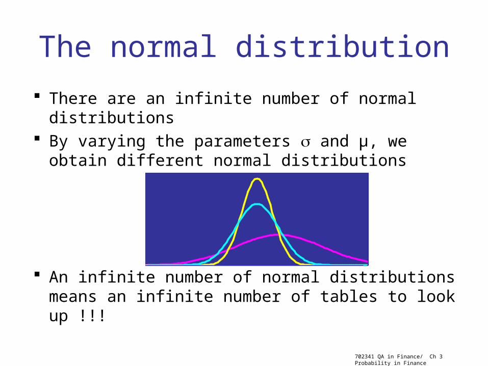
The normal distribution
There are an infinite number of normal distributions By varying the parameters and µ, we obtain
different normal distributions
An infinite number of normal distributions means an infinite number of tables to look up !!!

702341 QA in Finance/ Ch 3 Probability in Finance
Standardizing example
6.2 50.12
10
XZ
Normal Distribution
Standardized Normal
Distribution10 1Z
5 6.2 X Z0Z
0.12
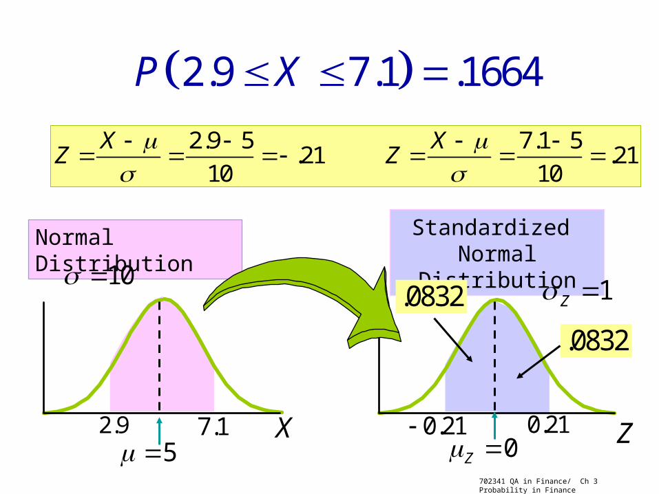
702341 QA in Finance/ Ch 3 Probability in Finance
Normal Distribution
Standardized Normal
Distribution10 1Z
5 7.1 X Z0Z
0.21
2.9 5 7.1 5.21 .21
10 10
X XZ Z
2.9 0.21
.0832
2.9 7.1 .1664P X
.0832

702341 QA in Finance/ Ch 3 Probability in Finance
Z .00 .01
0.0 .5000 .5040 .5080
.5398 .5438
0.2 .5793 .5832 .5871
0.3 .6179 .6217 .6255
.5832.02
0.1 .5478
Cumulative Standardized Normal Distribution Table (Portion) 0 1Z Z
Z = 0.21
2.9 7.1 .1664P X (continued)
0

702341 QA in Finance/ Ch 3 Probability in Finance
The normal distribution
Example:
We wish to know the probability of a given asset, which is assumed to have normally distributed returns, providing a return of between 4.9% and 5%. The mean of the return on that asset to date is 4%, and the standard deviation is 1%

702341 QA in Finance/ Ch 3 Probability in Finance
The normal distribution
Example:
The earnings of a company are expected to be $4.00 per share, with a standard deviation of $40. Assuming earnings per share are a continuous random variable that is normally distributed, calculate the probability of actual EPS will be $3.90 or higher.
702341 QA in Finance/ Ch 3 Probability in Finance
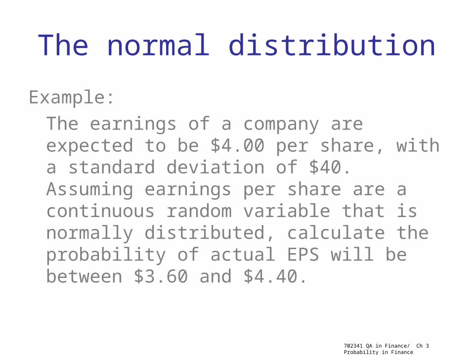
The normal distribution
Example:
The earnings of a company are expected to be $4.00 per share, with a standard deviation of $40. Assuming earnings per share are a continuous random variable that is normally distributed, calculate the probability of actual EPS will be between $3.60 and $4.40.
702341 QA in Finance/ Ch 3 Probability in Finance
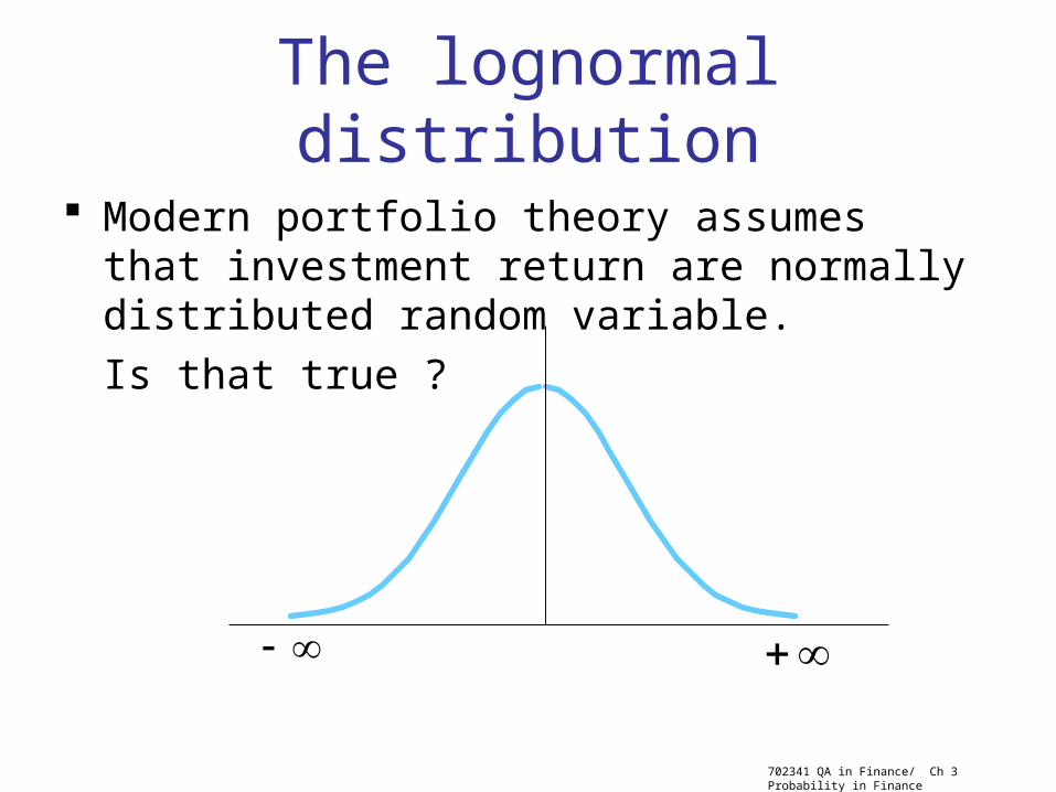
The lognormal distribution
Modern portfolio theory assumes that investment return are normally distributed random variable.
Is that true ?
702341 QA in Finance/ Ch 3 Probability in Finance
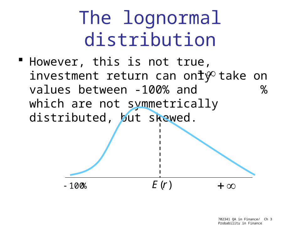
The lognormal distribution
However, this is not true, investment return can only take on values between -100% and % which are not symmetrically distributed, but skewed.
%100
)(rE
702341 QA in Finance/ Ch 3 Probability in Finance
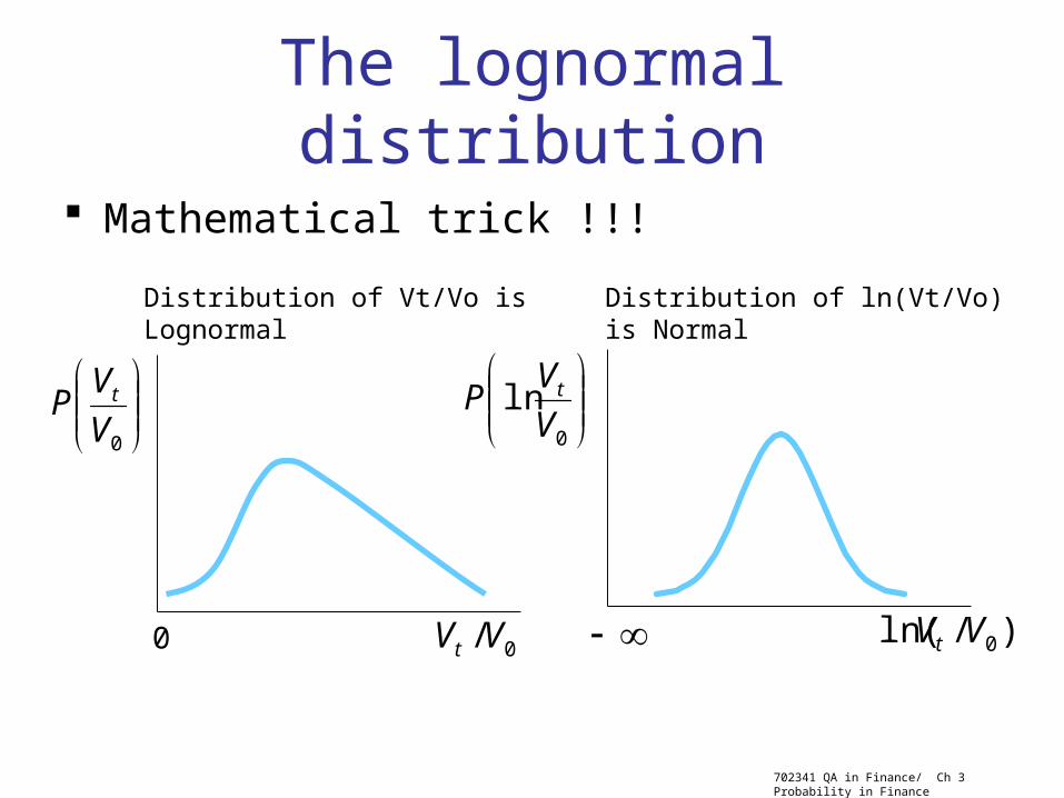
The lognormal distribution
Mathematical trick !!!
0 0/VVt
0V
VP t
)/ln( 0VVt
0
lnV
VP t
Distribution of Vt/Vo is Lognormal Distribution of ln(Vt/Vo) is Normal