
Statistical estimation, confidence intervals 1. 2 The central limit theorem.

7Statistical Intervals
Chapter 7 Stat 4570/5570
Material from Devore’s book (Ed 8), and Cengage

2
Confidence IntervalsThe CLT tells us that as the sample size n increases, thesample mean X is close to normally distributed withexpected value µ and standard deviation
Standardizing X by first subtracting its expected valueand then dividing by its standard deviation yields thestandard normal variable
How big does our sample need to be if the underlyingpopulation is normally distributed?

3
Basic Properties of Confidence Intervals
Because the area under the standard normal curvebetween –1.96 and 1.96 is .95, we know:
This is equivalent to:
which can be interpreted as the probability that the interval
includes the true mean µ is 95%.

4
Basic Properties of Confidence Intervals
The interval
is thus called the 95% confidence interval for the mean.
This interval varies from sample to sample, as thesample mean varies.
So the interval itself is a random interval.

5
Basic Properties of Confidence Intervals
The CI interval is centered at the sample mean X andextends 1.96 to each side of X.
The interval’s width is 2 (1.96) , which is notrandom; only the location of the interval (its midpoint X) israndom.

6
Basic Properties of Confidence Intervals
For a given sample, the CI can be expressed either as
or as
A concise expression for the interval is x ± 1.96 ,where – gives the left endpoint (lower limit) and + gives theright endpoint (upper limit).

7
Interpreting a Confidence LevelWe started with an event (that the random interval capturesthe true value of µ) whose probability was .95
It is tempting to say that µ lies within this fixed interval withprobability 0.95.
µ is a constant (unfortunately unknown to us). It istherefore incorrect to write the statement
P(µ lies in (a, b)) = 0.95
-- since µ either is in (a,b) or isn’t.
Basically, µ is not random (it’s a constant), so it can’t havea probability associated with its behavior.

8
Interpreting a Confidence LevelInstead, a correct interpretation of “95% confidence” relieson the long-run relative frequency interpretation ofprobability.
To say that an event A has probability .95 is to say that ifthe same experiment is performed over and over again, inthe long run A will occur 95% of the time.
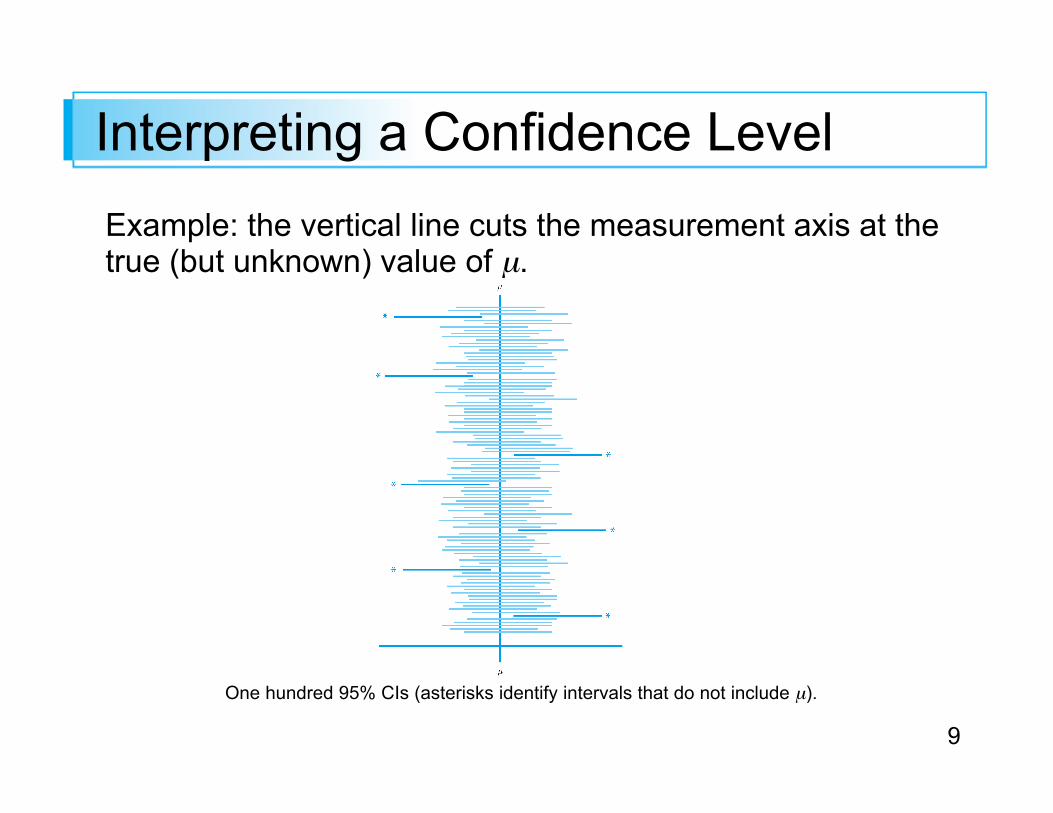
So the right interpretation is to say that in repeatedsampling, 95% of the confidence intervals obtained from allsamples will actually contain µ . The other 5% of theintervals will not.
9
Interpreting a Confidence LevelExample: the vertical line cuts the measurement axis at thetrue (but unknown) value of µ.
One hundred 95% CIs (asterisks identify intervals that do not include µ).

10
Interpreting a Confidence LevelAccording to this interpretation, the confidence level is nota statement about any particular interval, eg (79.3, 80.7).
Instead it pertains to what would happen if a very largenumber of like intervals were to be constructed using thesame CI formula.
11
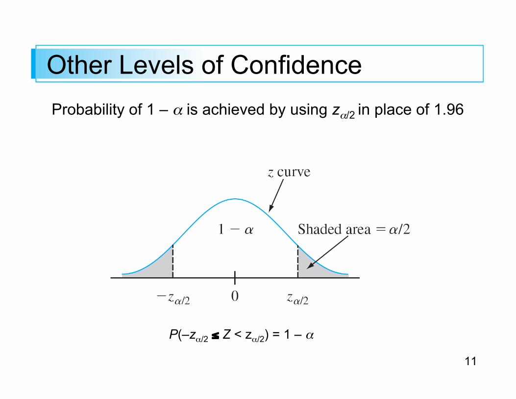
Other Levels of ConfidenceProbability of 1 – α is achieved by using zα/2 in place of 1.96
P(–zα/2 ≤ Z < zα/2) = 1 – α

12
Other Levels of ConfidenceA 100(1 – α)% confidence interval for the mean µ whenthe value of σ is known is given by
or, equivalently, by
The formula for the CI can also be expressed in words asPoint estimate ± (z critical value) (standard error).
13
ExampleA sample of 40 units is selected and diameter measured foreach one. The sample mean diameter is 5.426 mm, and thestandard deviation of measurements is 0.1mm.
Let’s calculate a confidence interval for true average holediameter using a confidence level of 90%. What is the widthof the interval?
What about the 99% confidence interval?
What are the advantages and disadvantages to a widerconfidence interval?

14
Sample size computationFor each desired confidence level and interval width, wecan determine the necessary sample size.
Example: A response time is normally distributed withstandard deviation 25 milliseconds. A new system hasbeen installed, and we wish to estimate the true averageresponse time µ for the new environment.
Assuming that response times are still normally distributedwith σ = 25, what sample size is necessary to ensure thatthe resulting 95% CI has a width of (at most) 10?

15
Unknown mean and varianceWe now have:
- a CI for the mean µ of a normal distribution- a large-sample CI for µ for any distribution
with a confidence level of 100(1 – α)% is:
A practical difficulty is the value of σ, which will rarely beknown. Instead we work with the standardized variable
Where the sample standard deviation S has replaced σ.

16
Unknown mean and variancePreviously, there was randomness only in the numerator ofZ by virtue of , the estimator.
In the new standardized variable, both and S vary invalue from one sample to another.
Thus the distribution of this new variable should be widerthan the Normal to reflect the extra uncertainty. This isindeed true when n is small.
However, for large n the subsititution of S for σ adds littleextra variability, so this variable also has approximately astandard normal distribution.

17
A Large-Sample Interval for µPropositionIf n is sufficiently large, the standardized variable
has approximately a standard normal distribution. Thisimplies that
is a large-sample confidence interval for µ withconfidence level approximately 100(1 – α)%.
This formula is valid regardless of the populationdistribution.
(7.8)
18
A Large-Sample Interval for µ
Generally speaking, n > 40 will be sufficient to justify theuse of this interval.
This is somewhat more conservative than the rule of thumbfor the CLT because of the additional variability introducedby using S in place of σ.

19
Small sample intervals for the mean
The CLT cannot be invoked when n is small• Need to do something else when n<40
•When n<40, we have to:• Make a specific assumption about the form of the
population distribution and• Derive a CI tailored to that assumption.
Example: Develop a CI for µ when the population isdescribed by a gamma distribution, another interval for thecase of a Weibull distribution, etc.

20
t Distributions

21
Intervals Based on a Normal Population Distribution
The result on which inferences are based introduces a newfamily of probability distributions called t distributions.
When is the mean of a random sample of size n from anormal distribution with mean µ, the rv
has a probability distribution called a t distribution with n – 1degrees of freedom (df).

22
Properties of t DistributionsFigure below illustrates some members of the t-family

23
Properties of t DistributionsProperties of t DistributionsLet tν denote the t distribution with ν df.
1. Each tν curve is bell-shaped and centered at 0.
2. Each tν curve is more spread out than the standard normal (z) curve.
3. As ν increases, the spread of the corresponding tν curve decreases.
4. As ν → , the sequence of tν curves approaches the standard normal curve (so the z curve is the t curve with df = ).

24
Properties of t DistributionsLet tα,ν = the number on the measurement axis for whichthe area under the t curve with ν df to the right of tα,ν is α;tα,ν is called a t critical value.
For example, t.05,6 is the t critical value that captures anupper-tail area of .05 under the t curve with 6 df

25
Tables of t DistributionsThe probabilities of t curves are found in a similar way asthe normal curve.
Example: obtain t.05,15

26
The One-Sample tConfidence Interval

27
The One-Sample t Confidence Interval
Let and s be the sample mean and sample standarddeviation computed from the results of a random samplefrom a normal population with mean µ. Then a100(1 – α)% confidence interval for µ is
or, more compactly

28
ExampleA dataset on the modulus of material rupture (psi):
6807.99 7637.06 6663.28 6165.03 6991.41 6992.236981.46 7569.75 7437.88 6872.39 7663.18 6032.286906.04 6617.17 6984.12 7093.71 7659.50 7378.617295.54 6702.76 7440.17 8053.26 8284.75 7347.957422.69 7886.87 6316.67 7713.65 7503.33 7674.99
There are 30 observations.The sample mean is 7203.191The sample standard deviation is 543.5400.
cont’d

29
Intervals Based on Nonnormal Population Distributions
The one-sample t CI for µ is robust to small or evenmoderate departures from normality unless n is very small.
By this we mean that if a critical value for 95% confidence,for example, is used in calculating the interval, the actualconfidence level will be reasonably close to the nominal 95%level.
If, however, n is small and the population distribution isnon-normal, then the actual confidence level may beconsiderably different from the one you think you are usingwhen you obtain a particular critical value from the t table.

30
A Confidence Interval for aPopulation Proportion

31
A Confidence Interval for a Population Proportion
Let p denote the proportion of “successes” in a population.
A random sample of n individuals is to be selected, and Xis the number of successes in the sample.X can be thought of as a sum of all Xi’s, where 1 is addedfor every success that occurs and a 0 for every failure, soX1 + . . . + Xn = X).
Thus, X can be regarded as a binomial rv with mean npand .
If both np ≥ 10 and n(1-p) ≥ 10, X has approximately anormal distribution.

32
A Confidence Interval for a Population Proportion
The natural estimator of p is = X / n, fraction of successes.Since is the sample mean, (X1 + . . . + Xn)/ n has approximately a normal distribution. We know that,E( ) = p (unbiasedness) and .
The standard deviation involves the unknown parameterp. Standardizing by subtracting p and dividing by thenimplies that
And the CI is

33
One-Sided Confidence Intervals

34
One-Sided Confidence Intervals (Confidence Bounds)
The confidence intervals discussed thus far give both alower confidence bound and an upper confidence bound forthe parameter being estimated.
In some circumstances, an investigator will want only oneof these two types of bounds.
For example, a psychologist may wish to calculate a 95%upper confidence bound for true average reaction time to aparticular stimulus, or a reliability engineer may want only alower confidence bound for true average lifetime ofcomponents of a certain type.

35
One-Sided Confidence Intervals (Confidence Bounds)
Because the cumulative area under the standard normalcurve to the left of 1.645 is .95,
Manipulating the inequality inside the parentheses toisolate µ on one side and replacing rv’s by calculatedvalues gives the inequality µ > – 1.645s/
The expression on the right is the desired lower confidencebound.

36
One-Sided Confidence Intervals (Confidence Bounds)
Starting with P(–1.645 < Z) ≈ .95 and manipulating theinequality results in the upper confidence bound. A similarargument gives a one-sided bound associated with anyother confidence level.
PropositionA large-sample upper confidence bound for µ is
and a large-sample lower confidence bound for µ is
37
Confidence Intervals for Varianceof a normal population
38
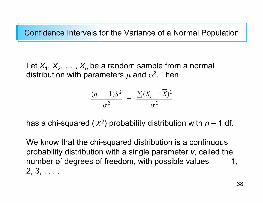
Confidence Intervals for the Variance of a Normal Population
Let X1, X2, … , Xn be a random sample from a normaldistribution with parameters µ and σ2. Then
has a chi-squared ( 2) probability distribution with n – 1 df.
We know that the chi-squared distribution is a continuousprobability distribution with a single parameter v, called thenumber of degrees of freedom, with possible values 1,2, 3, . . . .
39
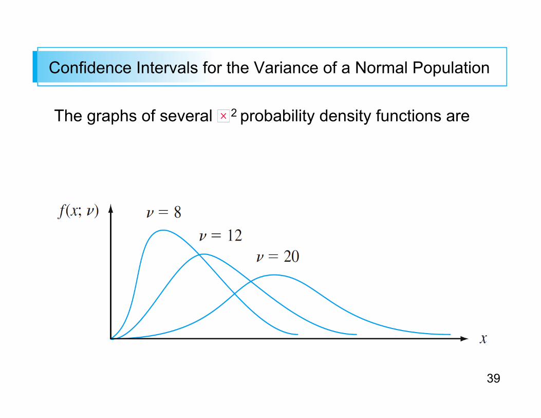
Confidence Intervals for the Variance of a Normal Population
The graphs of several 2 probability density functions are
40
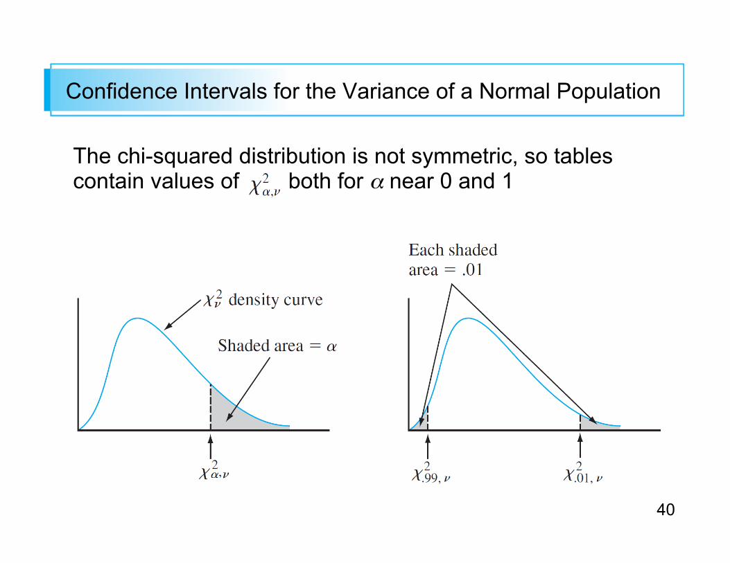
Confidence Intervals for the Variance of a Normal Population
The chi-squared distribution is not symmetric, so tablescontain values of both for α near 0 and 1

41
Confidence Intervals for the Variance of a Normal Population
As a consequence
Or equivalently
Substituting the computed value s2 into the limits gives a CIfor σ2
Taking square roots gives an interval for σ.

42
Confidence Intervals for the Variance of a Normal Population
A 100(1 – α)% confidence interval for the variance σ2 ofa normal population has lower limit
and upper limit
A confidence interval for σ has lower and upper limits thatare the square roots of the corresponding limits in theinterval for σ2.

43
ExampleThe data on breakdown voltage of electrically stressedcircuits are:
breakdown voltage isapproximately normallydistributed.