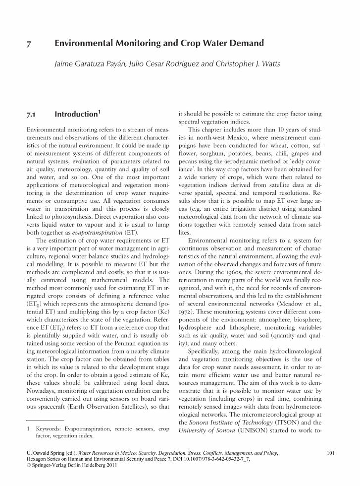
7 Environmental Monitoring and Crop Water Demand

Jaime Garatuza Payán, Julio Cesar Rodríguez and Christopher J. Watts

7.1 Introduction1

Environmental monitoring refers to a stream of meas-urements and observations of the different character-istics of the natural environment. It could be made upof measurement systems of different components ofnatural systems, evaluation of parameters related toair quality, meteorology, quantity and quality of soiland water, and so on. One of the most importantapplications of meteorological and vegetation moni-toring is the determination of crop water require-ments or consumptive use. All vegetation consumeswater in transpiration and this process is closelylinked to photosynthesis. Direct evaporation also con-verts liquid water to vapour and it is usual to lumpboth together as evapotranspiration (ET).

The estimation of crop water requirements or ETis a very important part of water management in agri-culture, regional water balance studies and hydrologi-cal modelling. It is possible to measure ET but themethods are complicated and costly, so that it is usu-ally estimated using mathematical models. Themethod most commonly used for estimating ET in ir-rigated crops consists of defining a reference value(ET0) which represents the atmospheric demand (po-tential ET) and multiplying this by a crop factor (Kc)which characterizes the state of the vegetation. Refer-ence ET (ET0) refers to ET from a reference crop thatis plentifully supplied with water, and is usually ob-tained using some version of the Penman equation us-ing meteorological information from a nearby climatestation. The crop factor can be obtained from tablesin which its value is related to the development stageof the crop. In order to obtain a good estimate of Kc,these values should be calibrated using local data.Nowadays, monitoring of vegetation condition can beconveniently carried out using sensors on board vari-ous spacecraft (Earth Observation Satellites), so that

it should be possible to estimate the crop factor usingspectral vegetation indices.

This chapter includes more than 10 years of stud-ies in north-west Mexico, where measurement cam-paigns have been conducted for wheat, cotton, saf-flower, sorghum, potatoes, beans, chili, grapes andpecans using the aerodynamic method or ‘eddy covar-iance’. In this way crop factors have been obtained fora wide variety of crops, which were then related tovegetation indices derived from satellite data at di-verse spatial, spectral and temporal resolutions. Re-sults show that it is possible to map ET over large ar-eas (e.g. an entire irrigation district) using standardmeteorological data from the network of climate sta-tions together with remotely sensed data from satel-lites.

Environmental monitoring refers to a system forcontinuous observation and measurement of charac-teristics of the natural environment, allowing the eval-uation of the observed changes and forecasts of futureones. During the 1960s, the severe environmental de-terioration in many parts of the world was finally rec-ognized, and with it, the need for records of environ-mental observations, and this led to the establishmentof several environmental networks (Meadow et al.,1972). These monitoring systems cover different com-ponents of the environment: atmosphere, biosphere,hydrosphere and lithosphere, monitoring variablessuch as air quality, water and soil (quantity and qual-ity), and many others.

Specifically, among the main hydroclimatologicaland vegetation monitoring objectives is the use ofdata for crop water needs assessment, in order to at-tain more efficient water use and better natural re-sources management. The aim of this work is to dem-onstrate that it is possible to monitor water use byvegetation (including crops) in real time, combiningremotely sensed images with data from hydrometeor-ological networks. The micrometeorological group atthe Sonora Institute of Technology (ITSON) and theUniversity of Sonora (UNISON) started to work to-1 Keywords: Evapotranspiration, remote sensors, crop

factor, vegetation index.

© Springer-Verlag Berlin Heidelberg 2011 DOI 10.1007/978-3-642-05432-7_7,

Water Resources in Mexico: Scarcity, Degradation, Stress, Conflicts, Management, and PolicyHexagon Series on Human and Environmental Security and Peace 7,Ú. Oswald Spring (ed.), , 101

102 Jaime Garatuza Payán, Julio Cesar Rodríguez and Christopher J. Watts

gether about 15 years ago and results from this periodare presented here.

7.2 Meteorological Networks

Atmospheric and meteorological measurements havea long history in Mexico, going back several centuries.More recently, the National Meteorological Service(SNM) was established in 1901 with its own meteoro-logical observatories and stations transmitting cli-matic data by telegraph. Afterwards, SMN was ab-sorbed by the Ministry of Water Resources (SRH)and now is part of the National Water Commission(CONAGUA). An important responsibility of SMN isto maintain a national database and provide public ac-cess to meteorological and climatic information, aswell as the realization of other meteorological and cli-matic studies. Thus, the infrastructure maintained bySMN includes more than 3000 meteorological sta-tions, mostly manual, but including some automatedstations.

Given the importance of hydrometeorologicalmonitoring for agricultural activities and food produc-tion in Mexico, the federal Ministry of Agriculture(SAGARPA) has implemented a national network ofagro-climatological stations, providing real-time mete-orological data to help the agricultural sector and soimprove the competitiveness of agribusiness. This net-work provides information to support farmers inimproving their production, specifically in the applica-tion of irrigation water. The network contains morethan 850 stations situated throughout Mexico.

7.3 Remotely Sensed Data

The constellation of Earth Observation Satellites(EOS) constitutes another system for environmentalmonitoring. These satellites carry diverse sensors thatmake continual observations of the earth (without theneed to be in direct contact with it) in differentregions of the electromagnetic spectrum. The obser-vations consist of measurements of the energyreflected or emitted by objects on the earth’s surface,or above it (clouds). The interpretation of these meas-urements is based a) on the distinctive spectral signa-ture in which each object reflects the incident electro-magnetic waves or b) on the quantity of energyemitted by the object as a function of its temperature,in accordance with the Stefan-Boltzmann law. Manydifferent satellites and sensors have been used in envi-ronmental monitoring and table 7.1 shows a list (far

from complete) of satellites and sensors in commonuse in Mexico. Three regions of the electromagneticspectrum have been used most frequently: visible(VIS), near infrared (NIR) and thermal infrared(TIR). The minimum time between observations ofthe same site (temporal resolution) varies from 15 min-utes to 26 days. The smallest surface that can beobserved by a satellite sensor (spatial resolution) var-ies from 2 metres to 4 kilometres.

Generally, in the context of water use by vegetation,satellite remote sensors are mainly used to estimatethe photosynthetically active (‘green’) biomass presentat a particular site and to estimate the differencebetween the temperature of the vegetation and thetemperature of the surrounding air, since this differ-ence is related to the concept of vegetation waterstress. In order to monitor vegetation ‘greenness’,spectral vegetation indices are commonly used. Themost common is the Normalized Difference Vegeta-tion Index (NDVI; Rouse et al., 1974):

where ρNIR and ρR are reflectance for the near infra-red band and the red band, respectively.

Table 7.1: Characteristics of the principal satellites orsensors with possible application in theestimation of water use by vegetation. PANrefers to a panchromatic broad band with highspatial resolution. Source: Data from theauthors.

Satellite/Sensor

Spectral Bands

Resolution

Spatial Temporal

GOES TIR 4 km 15 min

VIS 1km 15 min

MODIS VIS/NIR 250 m, 500 m

1-2 days

TIR 1 km 1-2 days

Landsat VIS/PAN 30 m / 15 m 16 days

TIR 60 m 16 das

SPOT VIS/PAN 10 m / 5 m 5-26 days

FORMOSAT VIS/PAN 8 m / 2 m 3-5 days

( )( )RNIR

RNIRNDVIρρρρ

+−=

Environmental Monitoring and Crop Water Demand 103

7.4 Environmental Monitoring with Remote Sensors

There are many examples of the use of remote sens-ing for environmental monitoring in Mexico. Forexample, Lobell et al. (2003) describe their experi-ence using LANDSAT data to estimate wheat yields inthe Yaqui valley, Sonora. Rodriguez et al. (2001, 2003,2004) investigated the possibility of using MODISdata to forecast yields for 80 ha of wheat. Lobell andAsnar (2004) developed and tested a linear disaggre-gation approximation to estimate the fractional coverof different crops in one MODIS pixel, based on timeseries of spectral signatures during the growing sea-son. They applied the technique in the Yaqui valley inMexico and in the southern Great Plains in the USA,demonstrating the importance of sub-pixel heteroge-neity in crop systems and the potential of temporaldisaggregation for providing fast, reliable estimates ofthe spatial distribution of land cover using low spatialresolution images like MODIS.

Hudson and Colditz (2003) combined remotelysensed and geomorphic data to delineate the spatialextent of flooding in the lower Panuco River causedby a large hurricane in the Gulf of Mexico. Salinas-Zavala et al. (2002) analysed the relationship betweenthe inter-annual variability of NDVI, rainfall andatmospheric circulation at 700 mb in northwest Mex-ico. They separated the data corresponding to thecold and warm phases of El Niño Southern Oscilla-tion (ENSO) and found that the negative phase ofENSO was associated with drought conditions.

The application of remotely sensed data for esti-mating hydrological variables has a long tradition. In

the early 1990s, Garatuza and Watts (1993) used VISand IR data from the geostationary satellite GOES toestimate the extent of snow cover in the westernSierra Madre, and constructed a computational sys-tem for estimating other variables using GOES imagesprovided by a receiving station installed at ITSON inCiudad Obregon, Sonora (Stewart et al., 1995). TheseGOES images were used by Yucel et al. (1998) andGaratuza et al. (2001a) to obtain high resolution mapsof cloudiness. Another application was the estimationof incoming solar radiation using GOES images fromthe receiving station at ITSON (Watts et al., 1995;Watts et al., 1999; Stewart et al., 1999; Garatuza et al.,2001b, 2001c). These studies provided new informa-tion about cloud cover in north-west Mexico and theuse of this information in a new method of obtaininghigh resolution estimates for incoming solar radiation,an important variable in environmental monitoringfor hydrological studies and integrated water manage-ment.

With regard to measurement, modelling, and esti-mation of evapotranspiration as an indicator of cropwater requirements, various studies have been pub-lished (Garatuza et al., 1998, 2001d, 2003, 2005b;Garatuza and Watts, 2005; Mendez-Barroso et al.,2008; Unland et al., 1997), combining data collectedin situ with remotely-sensed data of high and low spa-tial resolution (figures 7.1, 7.2). Additionally, experi-ments have been conducted to establish methods ofestimating average surface fluxes over heterogeneoussurfaces (Watts et al., 2001; Chehbouni et al., 2001,2008).

Figure 7.1: a) Real colour composite and b) evapotranspiration (W m-2) for wheat in the Yaqui valley, Mexico for oneday during the growing season of 2000. Source: Landsat bands 1, 2 and 3.

104 Jaime Garatuza Payán, Julio Cesar Rodríguez and Christopher J. Watts

7.5 Crop Water Requirements

The estimation of crop water needs or evapotranspi-ration (ET) is an important issue in water manage-ment in irrigated agriculture, regional water balancestudies and hydrological modelling. At the plot scale,estimates of ET are needed for irrigation schedulingand so form an integral part of decision support man-agement tools (Abrahamsen/Hansen, 2000; Gara-tuza/Watts, 2005).

It is possible to measure the rate of ET in situ, butthe equipment is expensive and the data collected inthe field requires complicated processing procedures.For this reason, ET for irrigated crops is usually esti-mated as the product of reference ET (ET0) that rep-resents the ‘atmospheric demand’ and a crop coeffi-cient Kc that reflects the vegetation condition(Garatuza/Watts, 2005):

ET = Kc * ET0

where ET0 refers to an “actively growing, well wateredgrassland (i.e. zero water stress) that completely cov-ers the ground”. ET0 is usually calculated with someversion of the Penman equation (Penman, 1948) thatrequires information about net radiation, air tempera-ture and humidity, and wind speed. Unfortunately,many versions of this equation have been proposedand the method is sometimes not applied correctly,but the publication of FAO-56 (Allen et al., 1998) pro-vides a convenient standardized version. So the cor-rect estimation of ET requires the following data:characteristics and development stage of the crop, cli-mate parameters, and management practices. The cli-

mate parameters are included in ET0 while the othersare included in the crop factor Kc.

7.5.1 Measurement and Estimation of Kc

The aforementioned factors are specific to each cropand change with crop development. Allen at al. (1998)subdivide the development stages of the crop intofour phases: initial, development, stabilization andsenescence, and presents tables with values of thesecoefficients for a large variety of crops, while recom-mending local calibration of the values. A great dealof work has been carried out to determine appropri-ate crop factors for different crops in different regionsusing different management practices. The determina-tion of accurate estimates of Kc requires measurementof actual ET and the estimation (using climatic varia-bles) of ET0 so that

Kc = ET/ET0

Some examples of the determination of Kc for differ-ent types of crops (annual, perennial, fruit trees, etc.)using different management practices (flood irriga-tion, drip irrigation, etc.) include Garatuza et al.(1998) who developed time dependent Kc for wheatand cotton under flood irrigation in the Yaqui valleybased on eddy covariance (EC) measurements of ac-tual ET; Benli et al. (2006), who used a weighinglysimeter to determine Kc for alfalfa in the semi-aridconditions of the Anatolian plains in Turkey; andWanga et al. (2007), who used four different methodsfor measuring ET in an open pecan orchard to de-

Figure 7.2: Annual evapotranspiration in Sonora (a) October 1999 to September 2000 using NOAA-AVHRR imagesand (b) October 2002 to September 2003 using MODIS images. The outlines of municipal limits have beenincluded. Source: Elaborated by the authors.

Environmental Monitoring and Crop Water Demand 105

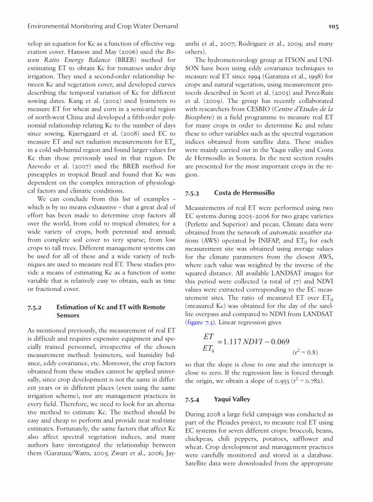
velop an equation for Kc as a function of effective veg-etation cover. Hanson and May (2006) used the Bo-wen Ratio Energy Balance (BREB) method forestimating ET to obtain Kc for tomatoes under dripirrigation. They used a second-order relationship be-tween Kc and vegetation cover, and developed curvesdescribing the temporal variation of Kc for differentsowing dates. Kang et al. (2002) used lysimeters tomeasure ET for wheat and corn in a semi-arid regionof north-west China and developed a fifth-order poly-nomial relationship relating Kc to the number of dayssince sowing. Kjaersgaard et al. (2008) used EC tomeasure ET and net radiation measurements for EToin a cold sub-humid region and found larger values forKc than those previously used in that region. DeAzevedo et al. (2007) used the BREB method forpineapples in tropical Brazil and found that Kc wasdependent on the complex interaction of physiologi-cal factors and climatic conditions.

We can conclude from this list of examples –which is by no means exhaustive – that a great deal ofeffort has been made to determine crop factors allover the world, from cold to tropical climates; for awide variety of crops, both perennial and annual;from complete soil cover to very sparse; from lowcrops to tall trees. Different management systems canbe used for all of these and a wide variety of tech-niques are used to measure real ET. These studies pro-vide a means of estimating Kc as a function of somevariable that is relatively easy to obtain, such as timeor fractional cover.

7.5.2 Estimation of Kc and ET with Remote Sensors

As mentioned previously, the measurement of real ETis difficult and requires expensive equipment and spe-cially trained personnel, irrespective of the chosenmeasurement method: lysimeters, soil humidity bal-ance, eddy covariance, etc. Moreover, the crop factorsobtained from these studies cannot be applied univer-sally, since crop development is not the same in differ-ent years or in different places (even using the sameirrigation scheme), nor are management practices inevery field. Therefore, we need to look for an alterna-tive method to estimate Kc. The method should beeasy and cheap to perform and provide near real-timeestimates. Fortunately, the same factors that affect Kcalso affect spectral vegetation indices, and manyauthors have investigated the relationship betweenthem (Garatuza/Watts, 2005; Zwart et al., 2006; Jay-

anthi et al., 2007; Rodriguez et al., 2009; and manyothers).

The hydrometeorology group at ITSON and UNI-SON have been using eddy covariance techniques tomeasure real ET since 1994 (Garatuza et al., 1998) forcrops and natural vegetation, using measurement pro-tocols described in Scott et al. (2003) and Perez-Ruizet al. (2009). The group has recently collaboratedwith researchers from CESBIO (Centre d’Etudes de laBiosphere) in a field programme to measure real ETfor many crops in order to determine Kc and relatethese to other variables such as the spectral vegetationindices obtained from satellite data. These studieswere mainly carried out in the Yaqui valley and Costade Hermosillo in Sonora. In the next section resultsare presented for the most important crops in the re-gion.

7.5.3 Costa de Hermosillo

Measurements of real ET were performed using twoEC systems during 2005–2006 for two grape varieties(Perlette and Superior) and pecan. Climate data wereobtained from the network of automatic weather sta-tions (AWS) operated by INIFAP, and ET0 for eachmeasurement site was obtained using average valuesfor the climate parameters from the closest AWS,where each value was weighted by the inverse of thesquared distance. All available LANDSAT images forthis period were collected (a total of 17) and NDVIvalues were extracted corresponding to the EC meas-urement sites. The ratio of measured ET over ET0(measured Kc) was obtained for the day of the satel-lite overpass and compared to NDVI from LANDSAT(figure 7.3). Linear regression gives

(r2 = 0.8)

so that the slope is close to one and the intercept isclose to zero. If the regression line is forced throughthe origin, we obtain a slope of 0.953 (r2 = 0.782).

7.5.4 Yaqui Valley

During 2008 a large field campaign was conducted aspart of the Pleiades project, to measure real ET usingEC systems for seven different crops: broccoli, beans,chickpeas, chili peppers, potatoes, safflower andwheat. Crop development and management practiceswere carefully monitored and stored in a database.Satellite data were downloaded from the appropriate

069.0117.10

−= NDVIETET

106 Jaime Garatuza Payán, Julio Cesar Rodríguez and Christopher J. Watts

websites for Landsat, MODIS and GOES. The FrenchSpace Agency CNES (Centre National d’Etudes Spa-tiales) provided 40 images from the FORMOSAT sat-ellite (8 metre spatial resolution) and NDVI valueswere extracted from these for each EC measurementsite. ET0 was calculated from data using the closestAWS (Block 1418) and Kc was calculated as the ratioof measured ET over ET0. Figure 7.4 presents theresults of relating measured Kc to NDVI. The slopeand intercept for the linear regression line is shownfor each crop. In each case, a line with slope equal to1 provides a good approximation to the observeddata, although not always the best one.

7.5.5 Spatial Distribution of Variables

In general, the measured values of ET and other me-teorological parameters are representative of only asmall area around the instrumented site. In contrast,the satellite images provide data for a large areaaround the site, so that they can be used to extrapo-late the calibrated results at the measurement sites.The linear relationship expressing Kc as a function ofNDVI can be used with GIS map algebra to obtainmaps of Kc. Similarly, if a map of ET0 is generated byinterpolation between the values for each AWS in thearea, then we can obtain a map of real ET as well. Fig-

ure 7.5 shows results for part of the Yaqui valley irriga-tion area for three days during the wheat-growing cy-cle in 2008. Only values for areas planted with wheatare shown and other crops have been masked out.The first column corresponds to 3 January at the be-ginning of the growing season, when the value is low(even zero in some places). The second column corre-sponds to 23 February when wheat is fully developedin the whole area, and the third column correspondsto 27 April in the final stage of the growing season,when most of the crop has become senescent. Notethe distinctive ‘stain’ in the upper left of the images.In this zone, some external factors had prevented thecrop from developing normally as in the rest of thearea.

In the first row, NDVI maps obtained from For-mosat are shown for the three dates. The values ofNDVI are between 0 and 1, increasing with theamount of biomass on the surface. The second rowshows maps of Kc, and the third row contains mapsof actual ET (in mm d-1) for the same dates. In thesecond column (23 February) Kc and ET have theirhighest values, with Kc around 1 and ET about 5-7mm d-1, corresponding to fully developed crops. Bythe third date (27 April) the vegetation is almost dry,while other areas, with later sowing dates or varietieswith longer growing seasons, are still active. So both

Figure 7.3: Relation between Kc and NDVI for grapes in the Costa de Hermosillo during 2005 and 2006. The values ofKc were obtained using EC measurements of ET and ETo from local climate data. Source: Data elaboratedby the authors based on NDVI obtained from Landsat 5 images.

Environmental Monitoring and Crop Water Demand 107

Kc and ET show a wide variation: 0.2–0.8 and 2–7

mm d-1 respectively.

7.6 Conclusions

The estimation of water demand and use by crops isan important factor in the planning and operation ofirrigation systems and also in hydrological studies todetermine water availability in a region. Reliable meth-ods to determine these are costly and complicated, sothat it is common practice to use simple modelsinstead, the most common of which is the two-stagemodel proposed by FAO. In this model, first the ref-erence evapotranspiration (ET0) is calculated using cli-mate data collected from meteorological monitoringnetworks, and then the crop factor is determined.

The influences on crop factors are the same asthose that affect spectral vegetation indices, generallybased on the differences in the reflectance of the veg-etation and soil in the red and near infrared bands ofelectromagnetic radiation. Therefore, it is possible toestablish functional relationships between vegetationindices (VI) and crop factors (Kc), so that the latter

may be estimated using routine observations fromearth observation satellites.

The results of many studies carried out by theauthors suggest that Kc can be represented as a linearfunction of VI with slope close to unity. The interceptis variable and depends on crop type and percentagecover.

These results indicate that a family of linear equa-tions with unit slope and variable intercept (functionof crop type and cover) could be used to provide nearreal-time estimates of Kc and ET with the necessaryspatial and temporal resolution to be used operation-ally in irrigation scheduling. In order to accomplishthis, it is essential that the climate data and remotelysensed data (from satellite, aircraft or other plat-forms) be available on time and the results be availa-ble online, so that the end users receive the informa-tion in a timely fashion. It is also important tomaintain an up-to-date database with information oncrop types, sowing dates, application of irrigation, fer-tilizer, etc.

Figure 7.4: Relationship between Kc and NDVI for six different crops in the Yaqui valley in 2008. Kc values wereobtained from the ratio of measured ET (using EC systems) and ET0. NDVI was obtained from Formosatimages. The slope and intercept from linear regression are included for each crop. Source: Elaborated bythe authors.

108 Jaime Garatuza Payán, Julio Cesar Rodríguez and Christopher J. Watts

References

Abrahamsen, P. and S. Hansen (2000), “Daisy: an opensoil–crop–atmosphere system model. Environ”, inModel. Software, vol. 15, pp. 313–330.

Allen, R.G., L. S. Pereira, D. Raes and M. Smith (1998),Crop evapotranspiration. Guidelines for computingcrop water requirements, Rome, Food and AgricultureOrganization of the United Nations (FAO Irr. Drain,Paper 56).

Belousova, Anna P., Irina K Gavich, Aleksandr B. Lisenkovand Evgenii V. Popov (2006), in Hidrogeología ecológ-ica, Moscow, Russia, Editorial IKC Akademkniga.

Benli, B., S.Kodal, A. Ilbeyi and H. Ustun (2006), “Determi-nation of evapotranspiration and basal crop coefficient

of alfalfa with a weighing lysimeter”, in AgriculturalWater Management, vol. 81, pp. 358–370.

Chehbouni, A., C. Watts, J. C. Rodríguez, F. Santiago, J.Garatuza Payán and J. Schieldge (2001), “Area-estimatesof surface fluxes over a mosaic of agricultural fields”, inManfred Owe, Kaye Brubaker, Jerry Richtie and AlbertRango (eds.), Remote Sensing and Hydrology 2000,Proceedings of a symposium held at Santa Fe, NewMexico, April 2000 (IAHS Publ. no. 267), pp. 220–222.

Chehbouni, A., J. C. B. Hoedjes, J. C. Rodriquez, C. J.Watts, J. Garatuza, F. Jacob and Y. H. Kerr (2008),“Using remotely sensed data to estimate area-averageddaily surface fluxes over a semi-arid mixed agriculturalland“, in Agricultural and Forest Meteorology, vol. 148,pp. 330–342.

Figure 7.5: NDVI (row1), Kc (row2) and actual ET (row 3) for three dates during the growing season for wheat in theYaqui valley. Only values for the fields with wheat are shown; the others are blank. The three dates chosenare: 3 January (Column 1), 23 February (Column 2) and 23 April (Column 3). Source: Elaborated by theauthors.

Environmental Monitoring and Crop Water Demand 109

de Azevedo P. V., C. V. de Souza, B.B. da Silva and V. P. R.da Silva (2007), “Water requirements of pineapple cropgrown in a tropical environment”, in Brazil. AgriculturalWater Management, vol. 88, pp. 201–208.

Garatuza Payan, J. and C. J. Watts (1993), “El uso deImágenes de Satélite en la Estimación de AreasCubiertas por Nieve”, in Revista ITSON-DIEP, CiudadObregón, Mexico. vol. 1, no. 4, pp 3–15.

Garatuza Payán, J., W. J.Shuttleworth, D. Encinas, D. D.Mc.Neil, J. B. Stewart, H. deBruin and C. J. Watts (1998),“Measurement and Modelling Evaporation for IrrigatedCrops in Northwest Mexico”, in: Hydrological Proc-esses, vol. 12, pp. 1397–1418.

Garatuza Payan, J., R. T. Pinker and W. J. Shuttleworth(2001a), “High resolution day-time cloud observationsfor northwestern Mexico from GOES-7 satellite data”,in Journal of Atmospheric and Oceanic Technology,vol. 105, no. 1, pp. 39–56.

Garatuza Payan, J., W. J. Shuttleworth and R. Pinker(2001b), “Satelite measurements of solar radiation in theYaqui Valley, Northern Mexico”, in Geofísica Internac-ional, vol. 40, no. 3, pp. 207–218.

Garatuza Payan, J., R. T. Pinker, W. J. Shuttleworth and C.Watts (2001c), “Solar radiation and evapotranspirationin northern Mexico estimated from remotely sensedmeasurements of cloudiness”, in Hydrological SciencesJournal, vol. 46, no. 3, pp. 465–478.

Garatuza Payan, J., R. T. Pinker, W. J. Shuttleworth and C.Watts (2001d), “Remotely Sensed Estimates of Evapora-tion for Irrigated Crops In Northern Mexico”, in Man-fred Owe, Kaye Brubaker, Jerry Richtie and AlbertRango (eds.), Remote Sensing and Hydrology 2000,Proceedings of a symposium held at Santa Fe, NewMexico, April 2000, IAHS Publ., no. 267, pp. 286–291.

Garatuza Payan, J., A. Tamayo, C. Watts and J. C. Rodríguez(2003), “Estimating Large Area Wheat Evapotranspira-tion from Remote Sensing Data”, in: 2003 IEEE Inter-national Geoscience and Remote Sensing Symposium,vol. 1, pp. 380–382.

Garatuza Payan, J. and C. J. Watts (2005), “The use ofremote sensing for estimating ET in NW Mexico”, in:Irrigation and Drainage Systems, vol. 19, pp. 301–320.

Garatuza Payan, J., W. Bastiaanssen and C. Watts (2005),Estudio histórico de uso y extracción del agua subter-ránea en dos áreas-piloto del Estado de Sonora, Mexico,CONAGUA, Gerencia de Aguas Subterráneas, ReporteFinal.

Hanson, B. R. and D. M. May (2006), “Crop coefficientsfor drip-irrigated processing tomato”, in: AgriculturalWater Management, vol. 81, pp. 381–399.

Hudson, P. F. and R. R. Colditz (2003), “Flood delineationin a large and complex alluvial valley, lower Panucobasin, Mexico”, in Journal of Hydrology, vol. 280, pp.229–245.

Jayanthi, H., C. M. U. Neale and J. L. Wright (2007),“Development and validation of canopy reflectance-

based crop coefficient for potato”, in AgriculturalWater Management, vol. 88, pp. 235–246.

Kang, S., G. Binjie, D. Taisheng and J.Zhang (2002), “Cropcoefficient and ratio of transpiration of winter wheatand maize in a semi-humid region“, in AgriculturalWater Management, vol. 59, pp. 239–254.

Kjaersgaard, J. H., F. Plauborg, M. Mollerup, C. T. Petersenand S. Hansen (2008), “Crop coefficients for winterwheat in a sub-humid climate regime”, in: AgriculturalWater Management, vol. 95, pp. 918–924.

Lobell, D. B., G. P. Asner, J. I. Ortiz Monasterio and T. L.Benning (2003), “Remote sensing of regional crop pro-duction in the Yaqui Valley, Mexico: estimates anduncertainties“, in Agriculture, Ecosystems and Environ-ment, vol. 94, pp. 205–220.

Lobell, D. D. and G. P. Asner (2004), “Cropland distribu-tions from temporal unmixing of MODIS data”, inRemote Sensing of Environment, vol. 93, pp. 412–422.

Meadows, Danella H., Denis L. Meadows, Jorgen Randersand William W. Behrens III (1972), Limits to Growth,New York, Universe Books.

Mendez Barroso, L. A., J. Garatuza Payan and E. Vivoni(2008), “Quantifying Water Stress on Wheat usingRemote Sensing in the Yaqui Valley, Sonora, Mexico”, inAgricultural Water Management, vol. 95, no. 6, pp.725–736 <DOI: 10.1016/j.agwat.2008.01.016>.

Penman, H. L. (1948), Natural evaporation from openwater, bare soil, and grass, Proceedings of the RoyalSociety of London A193, pp. 120–143.

Perez-Ruiz, E. R., J. Garatuza Payan, C. J. Watts, J. C. Rod-riguez, E. A. Yepez-Gonzalez (2009), “Carbon dioxideand water vapor exchange in a tropical dry forest asinfluenced by the North American Monsoon System(NAMS)”, in: Journal of Arid Environments, vol. 74,no. 5, pp. 556–563.

Rodriguez, J. C., C. Watts, G. Maubert, J. Garatuza Payan,A.Tamayo, L. Palacios and E. Palacios (2001), “Moni-toreo de Cultivos Utilizando Imágenes Modis”, inGEOS, Unión Geofísica Mexicana, Reunión Anual2001, vol. 21, no. 3, p. 349.

Rodriguez, J. C., B. Duchemin, C. J. Watts, R. Hadria, J.Garatuza, A. Chehbouni, G. Boulet, M. Armenta and S.Er-Raki (2003), “Wheat Yields Estimation UsingRemote Sensing and Crop Modeling in Yaqui Valley inMexico”, in 2003 IEEE International Geoscience andRemote Sensing Symposium, vol. 4, pp. 2221–2223.

Rodriguez, J. C., B. Duchemin, R. Hadria, C. Watts, J.Garatuza, A. Chehbouni, S.Khabba, G. Bouletb, E. Pala-cios and A. Lahrounic (2004), “Wheat yield estimationusing remote sensing and the STICS model in the semi-arid Yaqui valley, Mexico”, in Agronomie, vol. 24, pp.295–304.

Rodriguez, J. C., J. Grageda, A. Castellanos Villegas, J. Rod-riguez Casas, J. Saiz Hernandez, C. J. Watts, J. GaratuzaPayan and V. Olivarrieta (2009), “Water use by perennialcrops in the lower Sonora watershed”, in Journal ofArid Environments (in review).

110 Jaime Garatuza Payán, Julio Cesar Rodríguez and Christopher J. Watts

Rouse, J. W., R. H. Haas, J. A. Schell, D. W. Deering (1974),“Monitoring vegetation systems in the Great Plains withERTS“, in: Proceeding of the 3rd Earth Resource Tech-nology Satellite (ERTS) Symposium, vol. 1, pp. 48–62.

Salinas-Zavala C. A., A. V. Douglas and H. F. Diaz (2002),“Inter-annual Variability of NDVI in Northwest Mexico.Associated Climatic Mechanisms and Ecological Impli-cations“, in Remote Sensing and Environment, vol. 82,no. 2–3: pp. 417–430.

Scott, R. L., C. Watts, J. Garatuza Payan, E. Edwards, D. C.Goodrich, D. Williams and W. J. Shuttleworth (2003),“The understory and overstory partitioning of energyand water fluxes in an open canopy, semiarid wood-land”, in Agricultural and Forrest Meteorology, vol. 114,pp. 127–139.

Stewart J. B., H. A. R. de Bruin, J. Garatuza Payan and C. J.Watts (1995), “Use of satellite data to estimate hydrolog-ical variables for northwest Mexico”, 21st Annual Con-ference of the International Society of Remote Sensing,Southampton, UK, pp. 91–98.

Stewart, J. B., C. J. Watts, J. C. Rodríguez, H. A. R. deBruin, A. R. van den Berg and J. Garatuza Payan (1999),“Use of satellite data to estimate radiation and evapora-tion for northwest Mexico”, in Agricultural Water Man-agement, vol. 38, pp. 181–193.

Unland, E. H., A. M. Arain, C..Harlow, P. R. Houser, J.Garatuza Payan, P. Scott, O. L. Sen and W. J. Shuttle-worth (1997), “Evaporation from a Riparian System in aSemi-Arid Environment”, in Hydrological Processes, vol.12, pp. 527–542.

Wanga, J., T. W. Sammis, A. A. Andales, L. J. Simmons, V.P. Gutschick and D. Miller (2007), “Crop coefficientsof open-canopy pecan orchards“, in Agricultural watermanagement, vol. 88, pp. 253–262.

Watts, C. J., J. C. Rodriguez, J. Garatuza Payan, H. A. R. deBruin and J. B. Stewart (1995), “Estimates of Solar Radi-ation from GOES data on Northwest Mexico”, 21stAnnual Conference of the International Society ofRemote Sensing, Southampton, UK, pp. 930–910.

Watts, C. J., J. C. Rodríguez, J. Garatuza Payán, H. A. R. deBruin and J. B. Stewart (1999), "Estimación deevaporación y radiación solar en el valle del Yaqui,Sonora, usando datos de satélite", in IngenieríaHidráulica en México, vol. XIV, no. 3, pp. 45–53.

Watts, C., A.Chehbouni, J. C. Rodríguez, F. Santiago, J.Garatuza Payán and J. Schieldge (2001), “Aggregationrules for sensible heat flux estimates over agriculturalfields in Mexico”, in Manfred Owe, Kaye Brubaker,Jerry Richtie and Albert Rango (eds.), Remote Sensingand Hydrology 2000, Proceedings of a symposium heldat Santa Fe, New Mexico, April 2000 (IAHS Publ. no.267), pp. 217–219.

Yucel, I., J. Garatuza Payan, J.J. Toth, J.J. Shuttleworth andR.T. Pinker (1998), “Cloud Screened Surface RadiationEstimates with High Resolution from Goes-9 Data”, inAmerican Meteorological Society, Special Symposiumon Hydrology, Phoenix, Arizona (Paper-P2.2).

Zwart, S. J., W.G.M. Bastiaanssen, J. Garatuza Payan andC.J. Watts (2006), “SEBAL For Detecting Spatial Varia-tion Of Water Productivity For Wheat In The Yaqui Val-ley, Mexico”, in AIP Conference Proceedings, 23 August2006, vol. 852, pp. 154–161.