7. Databases and Database Management Systems intermediate/Databases Int.pdf · 7. Databases and...

Comp Int Databases Notes (eac)

Flat File 2

P3 P2

Flat File 3

P4

Flat File 1

P1

Sales Dept. Marketing Dept. Supplies Dept.

7. Databases and Database Management Systems

7.1 What is a File?

A file is a collection of data or information that has a name, called the Filename. There are many different types of files:

Data files (e.g. a list of names and addresses of the members of a club)

Text files (e.g. a letter, a poem)

Program files (contain programs in machine language)

Directories (folders)

Other

7.2 Flat File System A Flat File is a data file that is not related to another file.

Diagram 1 (Flat File System: Each department has its own flat file and its own programs that access the files

7.3 Database System

A database is a set of related files that is created and managed by a

database management system (DBMS).


Diagram 2: A Database System i.e. all programs access the same

database. 7.4 Advantages and Disadvantages of a Flat File System

Advantages:

Easy to understand

Easy to implement

Less hardware and software requirements

Less skills set are required to hand flat database systems

Best for small databases

Disadvantages:

Less security

Easy to extract information

Data Inconsistency

Data Redundancy

Sharing of information is cumbersome task

Slow for huge database

Searching process is time consuming

P3 P2 P4 P1

Sales Dept. Marketing Dept. Supplies Dept.

File 2

File 3

File 1


7.5 Advantages and Disadvantages of Database Systems

Advantages:

Reduced data redundancy

Reduced updating errors and increased consistency

Greater data integrity and independence from applications programs

Improved data access to users through use of query languages

Improved data security

Reduced data entry, storage, and retrieval costs

Facilitated development of new applications program

Disadvantages:

Database systems are complex, difficult, and time-consuming to

design

Substantial hardware and software start-up costs

Damage to database affects virtually all applications programs

Extensive conversion costs in moving form a file-based system to

a database system

Initial training required for all programmers and users

7.6 The Database Management System (DBMS)

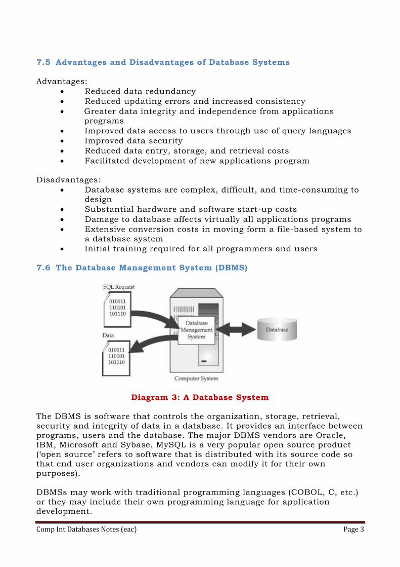
Diagram 3: A Database System The DBMS is software that controls the organization, storage, retrieval,

security and integrity of data in a database. It provides an interface between programs, users and the database. The major DBMS vendors are Oracle, IBM, Microsoft and Sybase. MySQL is a very popular open source product

(‘open source’ refers to software that is distributed with its source code so that end user organizations and vendors can modify it for their own

purposes). DBMSs may work with traditional programming languages (COBOL, C, etc.)

or they may include their own programming language for application development.


DBMSs let information systems be changed more easily as the

organization's requirements change. New categories of data can be added to the database without disruption to the existing system. Adding a field to a

record does not require changing any of the programs that do not use the data in that new field.

The major features of a DBMS are:

Data Security: The DBMS can prevent unauthorized users from

viewing or updating the database. Using passwords, users are allowed access to the entire database or a subset of it known as a "subschema." For example, in an employee database, some users may

be able to view salaries while others may view only work history and medical data.

Data Integrity: The DBMS can ensure that no more than one user can update the same record at the same time.

Interactive Query: A DBMS provides a query language and report writer that lets users interactively interrogate the database.

Interactive Data Entry and Updating: A DBMS typically provides a way to interactively enter and edit data.

Data Independence: The data inside the database is independent of the programs that use them or the users that access them. The

structure of data can change (e.g. a column added to a table, a value’s range changed, a string field length increased, etc.) without affecting the programs and the users’ operations.

7.7 Database Administrator (DBA)

The DBA is a person responsible for the physical design and management of the database and for the evaluation, selection and implementation of the DBMS.

In most organizations, the DBA and Data Administrator are one and the

same; however, when the two responsibilities are managed separately, the database administrator's function is more technical. Overall systems design decisions are performed by data administrators and systems analysts.

Detailed database design is performed by database administrators. 7.8 Relational Databases

There are many kinds of database models but one that is very frequently

used today is called a relational database. A relational database is a collection related tables. The relational database was invented by E. F. Codd at IBM in 1970.

In addition to being relatively easy to create and access, a relational database has the important advantage of being easy to extend. After the


original database creation, a new data category can be added without requiring that all existing applications (i.e. programs that make use of the

database) be modified.

Diagram 4: Nomenclature of Relational Databases

Each table (which is sometimes called a relation) contains one or more data

categories in columns. Each row contains a unique instance of data for the categories defined by the columns. For example, a typical business order entry database would include a table called Customer (with columns for

name, address, phone number, etc.) and a table called Order (with fields for product, customer, date, sales price, etc.).

A user of the database could obtain a view of the database that fitted the user's needs. For example, a branch office manager might like a view or

report on all customers that had bought products after a certain date. A financial services manager in the same company could, from the same tables, obtain a report on accounts that needed to be paid.

7.9 Relationships

Diagram 5 shows a database made up of two (unrelated) tables and diagram 6 shows the two tables that are now related to each other.

The attribute “ID NO.” in table “Student” is called the Primary Key because for each record this field has a unique value. This means there cannot be

two records in this table that have the same value for this field. Similarly for the table “Course”, “Course ID” is the primary field. The primary key is

sometimes called a Key Field. In diagram 6 the tables are related. The field “Course ID” in the Student

table has been introduced so as to create a relationship between the two tables. It is called a Foreign Key.


A primary key can be composite (also called compound) i.e. made up of more than one field. A Secondary Key is a non-primary key. For example “Name”

is a secondary key. However it is sometimes required to sort the records on this field.

Diagram 5: A Database of Two Unrelated Tables

Diagram 6: A Database of Two Related Tables


A relationship can be one of the following:

one-to-one

one-to-many (or many-to-one)

many-to-many

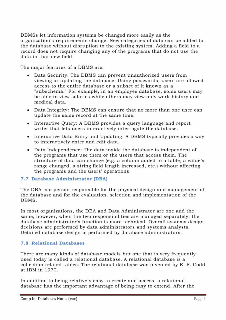
7.9.1 One-to-one This means that given two tables A and B each record in A can be

associated with only one record in B and similarly each record in B can be associated with only one record in table A. Look at the two examples in

diagram 7:

Diagram 7: One-to-one relationships

This means that each employee is assigned only one parking space and each parking space is assigned to only one employee. Likewise in the second

example each specialist is assigned only one ward and each ward is assigned to only one specialist.

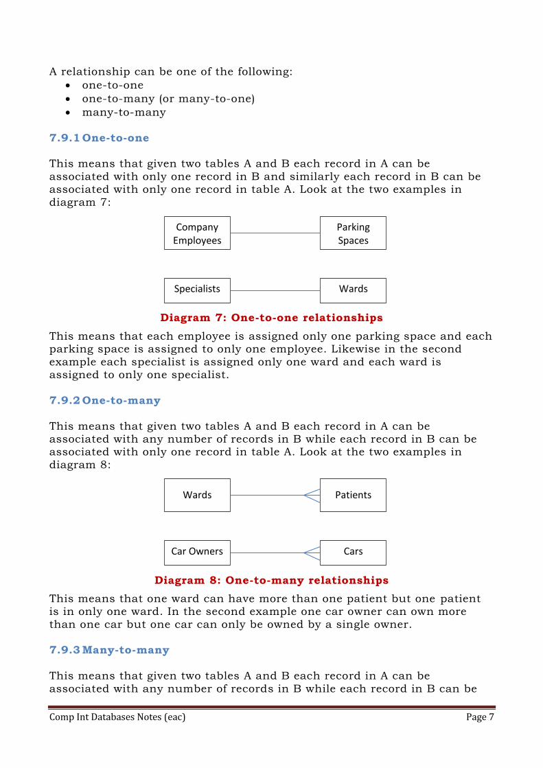
7.9.2 One-to-many

This means that given two tables A and B each record in A can be associated with any number of records in B while each record in B can be associated with only one record in table A. Look at the two examples in

diagram 8:

Diagram 8: One-to-many relationships

This means that one ward can have more than one patient but one patient is in only one ward. In the second example one car owner can own more

than one car but one car can only be owned by a single owner. 7.9.3 Many-to-many

This means that given two tables A and B each record in A can be

associated with any number of records in B while each record in B can be

Company Employees

Parking Spaces

Specialists Wards

Wards Patients

Car Owners Cars


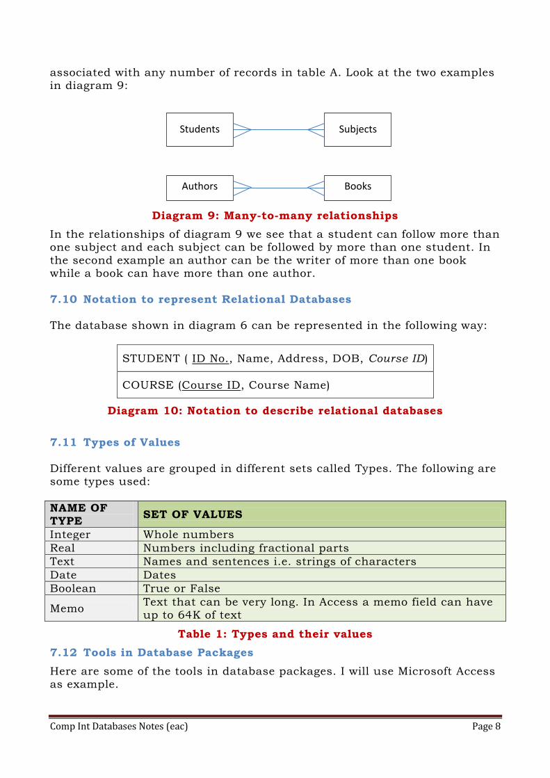
associated with any number of records in table A. Look at the two examples in diagram 9:

Diagram 9: Many-to-many relationships

In the relationships of diagram 9 we see that a student can follow more than one subject and each subject can be followed by more than one student. In

the second example an author can be the writer of more than one book while a book can have more than one author.

7.10 Notation to represent Relational Databases

The database shown in diagram 6 can be represented in the following way:

STUDENT ( ID No., Name, Address, DOB, Course ID)

COURSE (Course ID, Course Name)

Diagram 10: Notation to describe relational databases

7.11 Types of Values

Different values are grouped in different sets called Types. The following are some types used:

NAME OF

TYPE SET OF VALUES

Integer Whole numbers

Real Numbers including fractional parts

Text Names and sentences i.e. strings of characters

Date Dates

Boolean True or False

Memo Text that can be very long. In Access a memo field can have up to 64K of text

Table 1: Types and their values

7.12 Tools in Database Packages

Here are some of the tools in database packages. I will use Microsoft Access as example.

Students Subjects

Authors Books


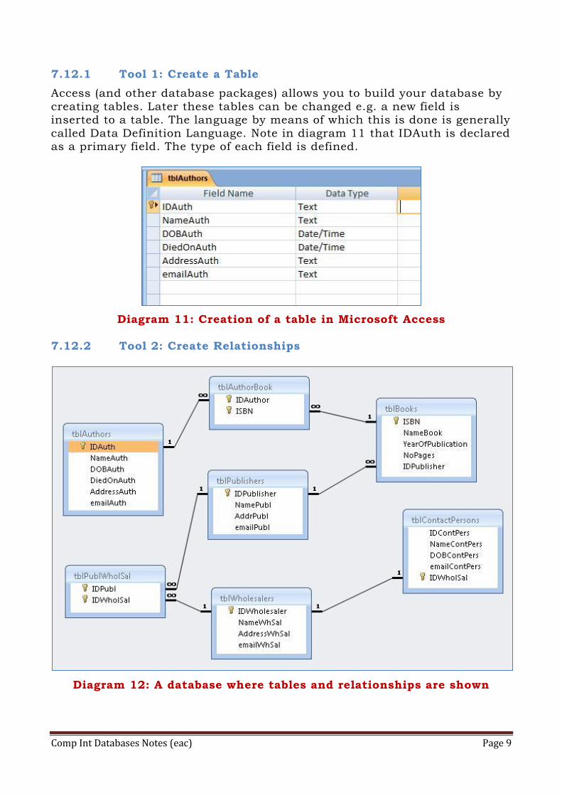
7.12.1 Tool 1: Create a Table

Access (and other database packages) allows you to build your database by

creating tables. Later these tables can be changed e.g. a new field is inserted to a table. The language by means of which this is done is generally

called Data Definition Language. Note in diagram 11 that IDAuth is declared as a primary field. The type of each field is defined.

Diagram 11: Creation of a table in Microsoft Access

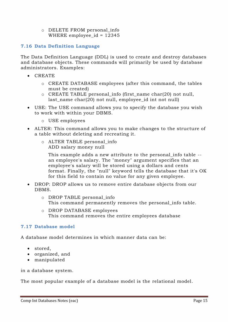
7.12.2 Tool 2: Create Relationships

Diagram 12: A database where tables and relationships are shown


Relationships can be 1-1 (one to one), 1-many (one to many; similarly we can have many to one) and many-many. This last relationship cannot be

directly represented in a relational database but this can be implemented by creating a third table. Diagram 12 shows a 1-1 relationship between

tblWholesalers and tblContactPersons. It also shows a 1-many relationship between tblPublishers and tblBooks. The many-many relationship between tblAuthors and tblBooks is implemented with the help of tblAuthorBook.

7.12.3 Tool 3: Referential Integrity

Referential Integrity is a condition that the designer of the database can include when defining a relationship. Let us explain it by means of an

example. In diagram 6, referential integrity would not let a student relate to a course that is not yet entered. Diagram 9 shows a case where a value would not be accepted when entered because referential integrity was

enforced when a relationship was created.

7.12.4 Tool 4: Validation Apart from referential integrity there are other times when values entered

are refused. These values can for example not be compatible with the type of the field. One example is when a field requires a number and text is entered instead. But apart from this obvious case the person constructing a table

can define validation rules. In such a way values are checked before they are accepted. One practical example is when a field of type date accepts only

values between two given dates.

Diagram 13: Referential integrity


7.12.5 Tool 5: Queries

Query by Example (see diagram 14) is one way to access data used by

Access Another way to devise a query is by using SQL (Structured Query Language). This is a query language devised for relational databases. An example is shown in diagram 15. Diagram 16 shows the resulting table of

the query. A Query extracts the required information from a database. So a query represents a virtual table. The tables that are created in the database are called Base Tables.

Diagram 14: Query by example

Diagram 15: SQL


Diagram 16: The result of the query shown in diagrams 14 and 15

7.12.6 Tool 6: Forms

A Form is a graphical arrangement that makes it easier to enter or view

records especially related records. See diagram 17. Note the subform (a form within a form) in the diagram. This subform shows related records.

Diagram 17: A Form


7.12.7 Tool 7: Reports

A report lists the results of a query or the contents of a table for the

purpose of printing. An Access report differs from a simple printout of a table's contents. When you create a report, you also can add headers,

footers, subtotals, and other special features that enhance the appearance of your data on the printed page. Using a report, you have complete control over how your information appears. See diagram 18.

Diagram 18: A Report

7.12.8 Some other tools

Other basic operations on tables are search, delete, modify and sort.

7.13 Data dictionary

A data dictionary is a file that defines the basic organization of a database. A data dictionary contains a list of all files in the database, the number of

records in each file, and the names and types of each field. Most database management systems keep the data dictionary hidden from users to prevent them from accidentally destroying its contents.

Data dictionaries do not contain any actual data from the database, only

bookkeeping information for managing it. Without a data dictionary, however, a database management system cannot access data from the database.


7.14 Query language

A query language is a specialized language for requesting information from a database. For example, the query

SELECT ALL WHERE age > 30 AND name = "Smith" requests all records in which the name-field is "Smith" and the Age field has a value greater than 30. The de facto standard for query languages is SQL.

7.15 Data Manipulation Language

The Data Manipulation Language (DML) is used to retrieve, insert and modify database information. These commands will be used by all database

users during the routine operation of the database. Let's take a brief look at the basic DML commands:

INSERT: The INSERT command in SQL is used to add records to an existing table. For example:

INSERT INTO personal_info values('bart','simpson',12345, $45000)

Note that there are four values specified for the record. These correspond to the table attributes in the order they were defined: first_name, last_name, employee_id, and salary.

SELECT: The SELECT command is the most commonly used command in SQL. It allows database users to retrieve the specific information

they desire from a database. Look at the following examples:

o SELECT * FROM personal_info

The above means "Select everything from the personal_info table."

o SELECT last_name FROM personal_info

The above command would show all values of the field

“last_name” from the table “personal_info”.

o SELECT *

FROM personal_info WHERE salary > $50000

UPDATE: The UPDATE command can be used to modify information

contained within a table, either in bulk or individually.

o UPDATE personal_info

SET salary = salary * 1.03

o UPDATE personal_info SET salary = salary + $5000

WHERE employee_id = 12345

DELETE


o DELETE FROM personal_info WHERE employee_id = 12345

7.16 Data Definition Language

The Data Definition Language (DDL) is used to create and destroy databases and database objects. These commands will primarily be used by database

administrators. Examples:

CREATE

o CREATE DATABASE employees (after this command, the tables must be created)

o CREATE TABLE personal_info (first_name char(20) not null,

last_name char(20) not null, employee_id int not null)

USE: The USE command allows you to specify the database you wish

to work with within your DBMS.

o USE employees

ALTER: This command allows you to make changes to the structure of a table without deleting and recreating it.

o ALTER TABLE personal_info ADD salary money null

This example adds a new attribute to the personal_info table --

an employee's salary. The "money" argument specifies that an employee's salary will be stored using a dollars and cents

format. Finally, the "null" keyword tells the database that it's OK for this field to contain no value for any given employee.

DROP: DROP allows us to remove entire database objects from our

DBMS.

o DROP TABLE personal_info

This command permanently removes the personal_info table.

o DROP DATABASE employees This command removes the entire employees database

7.17 Database model

A database model determines in which manner data can be:

stored,

organized, and

manipulated

in a database system.

The most popular example of a database model is the relational model.

http://en.wikipedia.org/wiki/Relational_model


7.17.1 Flat model

Diagram 19: A Flat-file model

The flat (or table) model consists of a single table. All members of a row are assumed to be related to one another.

7.17.2 Hierarchical model

In a hierarchical model, data is

organized into a tree-like structure. Hierarchical structures were widely used in the early mainframe

database management systems. This structure allows one 1:M relationship between two types of

data. This structure is very efficient to describe many relationships in

the real world. However, the hierarchical structure is inefficient for certain database operations.

Diagram 20: Hierachical model

7.17.3 Network model

The network model is a variation on the hierarchical model, to the

extent that it is built on the concept of multiple branches (lower-level structures) emanating

from one or more nodes (higher-level structures), while the model

differs from the hierarchical model in that branches can be connected to multiple nodes. The network

model is able to represent redundancy in data more efficiently than in the hierarchical model.

Diagram 21: Network Model

http://en.wikipedia.org/wiki/Flat_file_database

http://en.wikipedia.org/wiki/Hierarchical_database

http://en.wikipedia.org/w/index.php?title=File:Flat_File_Model.svg&page=1

http://en.wikipedia.org/w/index.php?title=File:Hierarchical_Model.svg&page=1

http://en.wikipedia.org/w/index.php?title=File:Network_Model.svg&page=1


7.17.4 Relational model

The relational model was introduced by E.F. Codd in 1970 as a way to make database management systems more independent of any particular application.

Three key terms are used extensively in relational database models:

relations, attributes, and domains. A relation (TABLE) is a table with columns and rows. The named columns of the relation are called attributes, and the domain is the set of values the attributes are allowed to take.

A relational database contains multiple tables, each similar to the one in the "flat" database model. Tables can also have a designated single attribute or a set of attributes that can act as a "key", which can be used to uniquely

identify each tuple in the table.

A key that can be used to uniquely identify a row in a table is called a primary key. Keys are commonly used to join or combine data from two or

more tables. Keys are also critical in the creation of indexes, which facilitate fast retrieval of data from large tables. Any column can be a key, or multiple columns can be grouped together into a compound key.

7.17.5 Object-oriented database models

Object oriented databases are also called Object Database Management Systems (ODBMS). Object databases store objects rather than data such as integers, strings or real numbers. Objects are used in object oriented

languages such as Smalltalk, C++, Java, and others. Objects basically consist of the following:

Attributes - Attributes are data which defines the characteristics of an

object.

Methods - Methods define the behaviour of an object and are what was

formally called procedures or functions.

An example of an object:

Cat: Attributes (i.e. how a cat can be described): age, name, breed, colour. Methods (i.e. what can a cat do?): run, eat, sleep.

Therefore objects contain both executable code and data.

Object databases work well with CASE Applications (CASE-computer aided software engineering, CAD-computer aided design, CAM-computer aided manufacture), Multimedia Applications and Commerce.

http://en.wikipedia.org/wiki/Relational_model

http://en.wikipedia.org/wiki/E.F._Codd

http://en.wikipedia.org/wiki/Relation_%28database%29

http://en.wikipedia.org/wiki/Data_domain


Object Database Advantages over RDBMS

Data model is based on the real world.

Less code required when applications are object oriented.

Object Database Disadvantages compared to RDBMS

Lower efficiency when data is simple and relationships are simple.

Relational tables are simpler.

7.18 Data Flow Diagram

A data flow diagram (DFD) is a graphical representation of the "flow" of data through an information system, modeling its process aspects. Often they are

a preliminary step used to create an overview of the system which can later be elaborated. DFDs can also be used for the visualization of data processing.

A DFD shows what kinds of information will be input to and output from the

system, where the data will come from and go to, and where the data will be stored.

DFDs only involve four symbols. They are: Process

Data Object Data Store External entity

These symbols are listed below:

Process Transform of incoming data flow(s) to outgoing flow(s).

Data Flow Movement of data in the system.

Data Store Data repositories for data that are not moving. It may be as simple as a buffer or a queue or as sophisticated as a relational

database.

External Entity Sources of destinations outside the specified system boundary.


The DFD may be used for any level of data abstraction. DFDs can be partitioned into levels. Each level has more information flow and data

functional details than the previous level.

Rules

In DFDs, all arrows must be labeled.

The information flow continuity, that is all the input and the output to

each refinement, must maintain the same in order to be able to produce a consistent system.

Strengths

DFDs have diagrams that are easy to understand, check and change data.

DFDs help tremendously in depicting information about how an organization operations.

They give a very clear and simple look at the organization of the interfaces between an application and the people or other applications that use it.

Weaknesses

Modification to a data layout in DFDs may cause the entire layout to

be changed. The number of units in a DFD in a large application is high. Therefore,

maintenance is harder, more costly and error prone. This is because

the ability to access the data is passed explicitly from one component to the other. This is why changes are impractical to be made on DFDs

especially in large system.

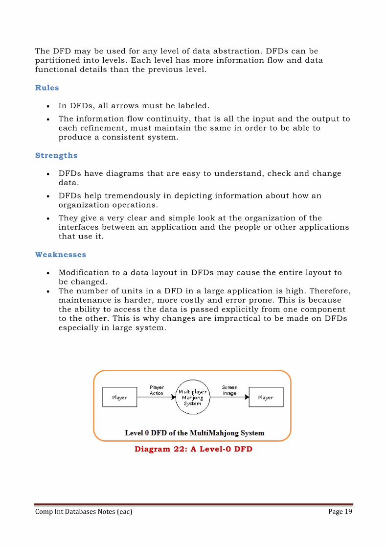
Diagram 22: A Level-0 DFD


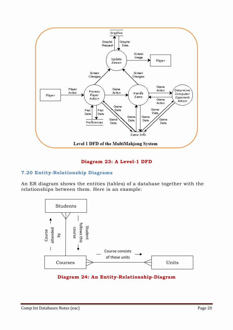
Diagram 23: A Level-1 DFD

7.20 Entity-Relationship Diagrams An ER diagram shows the entities (tables) of a database together with the

relationships between them. Here is an example:

Diagram 24: An Entity-Relationship-Diagram

Students

Courses Units

Co

urs

e

atte

nd

ed

by

Stud

ent

follo

ws th

is

cou

rse

Course consists

of these units


7.19 Normalisation

Normalisation is about properly designing your relational database. If you

ever find yourself in need to expand your database, or refactor it in order to fix or improve your existing applications, a proper design can save you an

enormous amount of time and effort. There are several steps involved in normalizing a database. The steps are

referred to as "Normal Forms" (abbreviated: NF). Tables that have reached the 3NF are generally considered "normalized".

Advantages & Disadvantages of Normalizing a Database

Advantages

Reduces Data Duplication

Groups Data Logically

Relationships are Represented Better

Disadvantages

Slows Database Performance

Requires Detailed Analysis and Design

Background to normalization: definitions Functional dependency

In a given table, an attribute Y is said to have a functional dependency on a

set of attributes X (written X → Y) if and only if each X value is associated with precisely one Y value. For example, in an "Employee" table that

includes the attributes "Employee ID" and "Employee Date of Birth", the functional dependency {Employee ID} → {Employee Date of Birth} would hold. It follows from the previous two sentences that each ‘Employee ID’ is

associated with precisely one ‘Employee Date of Birth’.

Superkey A superkey is a combination of attributes that can be used to uniquely

identify a database record. A table might have many superkeys. Let us consider an example of a university that consists of a number of

colleges. Each college gives an index number to each student. A table for all the university students might be the following:

Students (ID_No, College_No, Index_No, Name, Address, DOB)

All the following are superkeys: (ID_No, Name, DOB), (ID_No, College_No,

Name), (ID_No), (College_No, Index_No, DOB) etc. All the following are not superkeys: (Name, Address), (College_No, Name), (Index_No, Name) etc.

http://en.wikipedia.org/wiki/Functional_dependency

http://en.wikipedia.org/wiki/Superkey


Candidate key

A candidate key is a special subset of superkeys that do not have any extraneous information in them: it is a minimal superkey. In the above

example (ID_No) and (College_No, Index_No) are the only two candidate keys.

Non-prime attribute

A non-prime attribute is an attribute that does not occur in any candidate key. In the above example the non-prime attributes are Name, Address and

DOB.

Prime attribute A prime attribute, conversely, is an attribute that does occur in some

candidate key. The prime attributes in the example are ID_No, College_No and Index_No.

Primary key

One candidate key in a relation may be designated the primary key.

Denormalization

Denormalization (the opposite of normalisation) is also used to improve

performance on smaller computers as in computerized cash-registers and mobile devices, since these may use the data for look-up only (e.g. price lookups). Denormalization may also be used when no changes are to be made to the data

and a swift response is crucial. First Normal Form

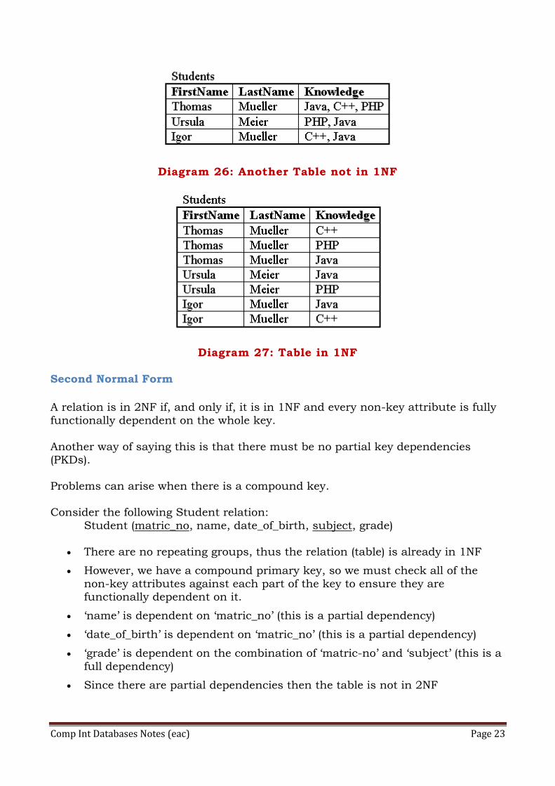
A relation is in 1NF if, and only if, it contains no repeating attributes or groups of

attributes. For example the following two tables are not in 1NF but the third one is.

Diagram 25: Table not in 1NF

http://en.wikipedia.org/wiki/Candidate_key

http://en.wikipedia.org/wiki/Primary_key


Diagram 26: Another Table not in 1NF

Diagram 27: Table in 1NF

Second Normal Form

A relation is in 2NF if, and only if, it is in 1NF and every non-key attribute is fully

functionally dependent on the whole key.

Another way of saying this is that there must be no partial key dependencies (PKDs).

Problems can arise when there is a compound key.

Consider the following Student relation:

Student (matric_no, name, date_of_birth, subject, grade)

There are no repeating groups, thus the relation (table) is already in 1NF

However, we have a compound primary key, so we must check all of the

non-key attributes against each part of the key to ensure they are functionally dependent on it.

‘name’ is dependent on ‘matric_no’ (this is a partial dependency)

‘date_of_birth’ is dependent on ‘matric_no’ (this is a partial dependency)

‘grade’ is dependent on the combination of ‘matric-no’ and ‘subject’ (this is a

full dependency)

Since there are partial dependencies then the table is not in 2NF


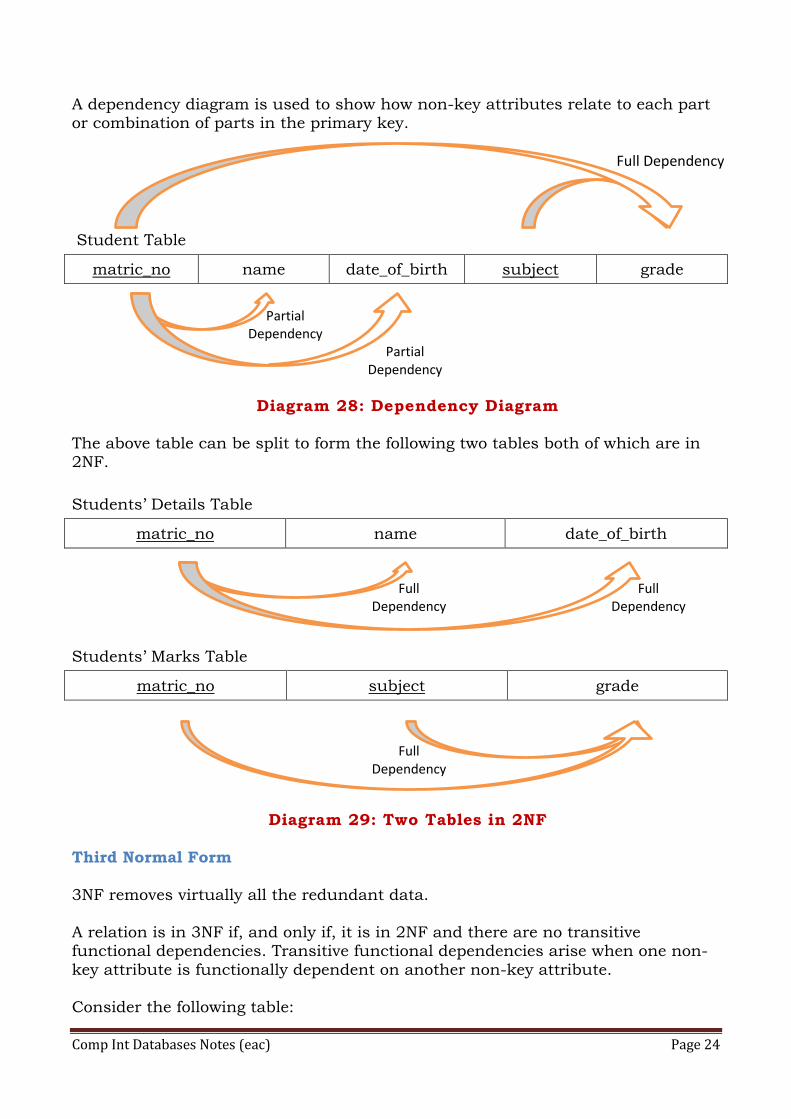
A dependency diagram is used to show how non-key attributes relate to each part or combination of parts in the primary key.

Student Table

matric_no name date_of_birth subject grade

Diagram 28: Dependency Diagram

The above table can be split to form the following two tables both of which are in 2NF.

Students’ Details Table

matric_no name date_of_birth

Students’ Marks Table

matric_no subject grade

Diagram 29: Two Tables in 2NF

Third Normal Form

3NF removes virtually all the redundant data.

A relation is in 3NF if, and only if, it is in 2NF and there are no transitive functional dependencies. Transitive functional dependencies arise when one non-

key attribute is functionally dependent on another non-key attribute.

Consider the following table:

Full Dependency

Partial Dependency

Partial Dependency

Full Dependency

Full Dependency

Full Dependency


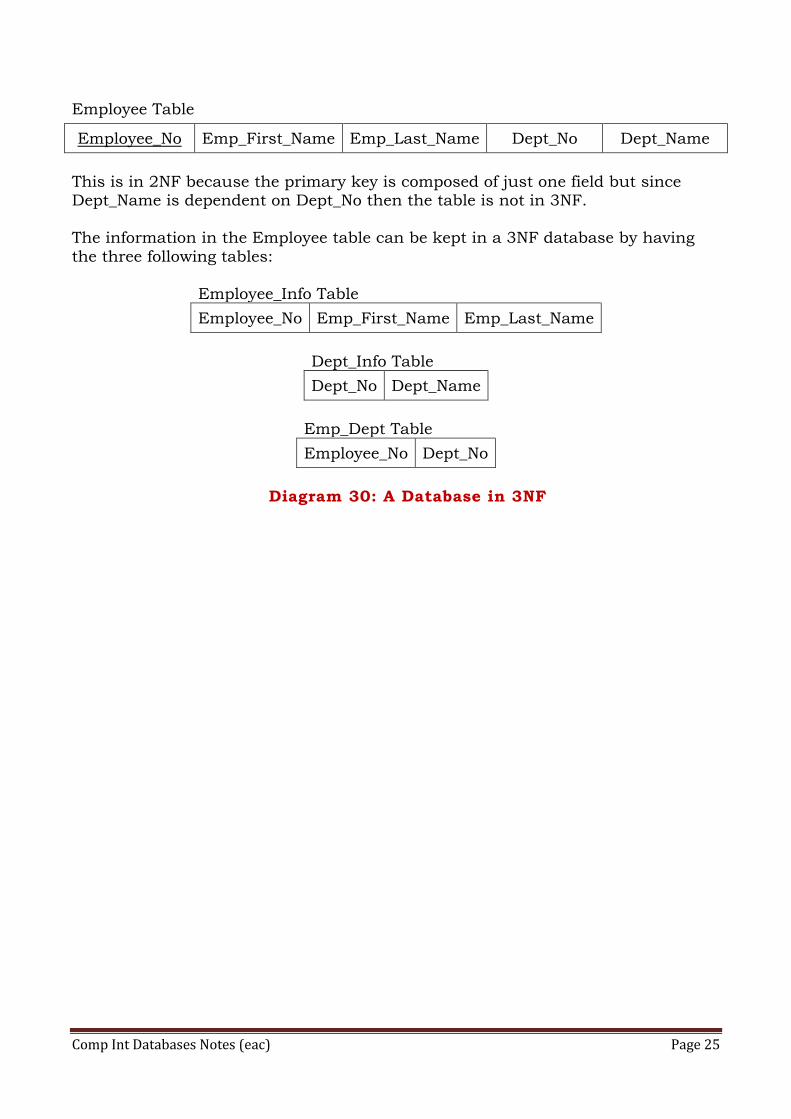
Employee Table

Employee_No Emp_First_Name Emp_Last_Name Dept_No Dept_Name

This is in 2NF because the primary key is composed of just one field but since Dept_Name is dependent on Dept_No then the table is not in 3NF.

The information in the Employee table can be kept in a 3NF database by having

the three following tables:

Employee_Info Table

Employee_No Emp_First_Name Emp_Last_Name

Dept_Info Table

Dept_No Dept_Name

Emp_Dept Table

Employee_No Dept_No

Diagram 30: A Database in 3NF

7. Databases and Database Management Systems intermediate/Databases Int.pdf · 7. Databases and...

Documents

Transcript of 7. Databases and Database Management Systems intermediate/Databases Int.pdf · 7. Databases and...