7 AD-AG93 299 MISSISSIPPI STATE UNIV MISSISSIPPI STATE ENGINEERING--ETC F/G 12/1

NUMERICAL GENERATION OF TWO-DIMENSIONAL ORTHOGONAL CURVILINEAR -ETC (U)JUN A0 Z U WARS I. R A WEED. J F THOMPSON AFOSR-8G-0185

UNCLASSIFIED MSSUEIRSASE-8G3 AFOSR-TA-AG 133Q

AFOSR-rjKR -80.-r13 39NUMERICAL GENERATION

OF AASETWO-DIMENSIONAL ORTHOGONAL 80- 213

CURVILINEAR COORDINATES

IN AN LVLEUCLIDEAN SPACE L V~

~mro

Department of Aerospace Engineering

by DTICZ. U. A. Warsi ELECTE

R.A. Weed, DEC 30 19M0J. F. Thomp~on SD

for ited.

Mississippi State University JUN 0 5 SoMississippi State, Mississippi 39762 MSSU-EIRS-ASE-80-3

COLLEGE OF ENGINEERING ADMINISTRATION

WILLIE L. MCDANIEL, PH.D.DEAN. COLLEGE OF ENGINEERING

WALTER R. CARNES, P11.0.ASSOCIATE DEAN

RALPH E. POWE, PH.D.ASSOCIATE DEAN

LAWRENCE J. HILL, M.S..DIRECTOR ENGINEERING EXTENSION

CHARLES 8. CLIETT, M.S.AEROSPACE ENGINEERING

WILLIAM R. FOX, PH.D.AGRICULTURAL & BIOLOGICAL ENGINEERING

JOHN L. WEEKS, JR., PH.D.CHEMICAL ENGINEERING

CIVIL ENGINEERING

B. J. BALL, PH.D.ELECTRICAL ENGINEERING

W. H. EUBANKS, M.ED.ENGINEERING GRAPHICS

FRANK E. COTTON, JR., PH.D. For additional copies or informatiorINDUTRIA ENINEEINGaddress correspondence to

C. T. CARLEY, PH.D.MECHANICAL ENGINEERING ENGINEERING AND INDUSTRIAL RESEARCH STATION

DRAWVER DEJOHN 1. PAULK, PH.D. MISSISSIPPI STATE UNIVERSITYNUCLEAR ENGINEERING MISSISSIPPI STATE MISSISSIPPI 39762

ELDRED W. HOUGH, PH.D.PETROLEUM ENGINEERING TELEPHONE 601) 325 2266

Missrssippi State University does nrot discriminate on lhe basis ol race colo reiiqo nation~al oriqinsex, age. or handrcap

In~ cornforrmity wiltr Title IX o1 the Educatiorn Amenldmenrts of 1972 and Section 5040 ofthe Rerr~atr,uirAct 0f1t973 Or T K Martirr Vice President 610 Allen Hall P 0 Drawer J. Mississippi Slate Mississippi39762 office telephone number 325-3221 has beern desigrrated as tlhe respoirsible orriflovee tocoordinate efforts to carry out responsibilities and make invcestigation ot complaints relatirr4 toirort isc ri mi nat in

*POR DOCMENTTIONPAGEREAL INSTRUCTIONS

1~AO R.8' 2. GVT ACCESSION No. 3. RECIPIENT'

STYPE: OF RE & PE-R- D COVERED[

6. P%:RMNG01G. REPoRr N &$ER

FCIDEAN PACE.7. AUIt~o9~ - -( S. CONTRACT OR GRANT NUMBER(.)

10 'Z. U. A.fWarsi R. A./ Weed J. F.17Thompson

9 PERFORMING ORGANIZ ATION NAME AND ADDRESS 10-w. PROGRAM ELEMENT. PROJECT. TASKAREA 6 WORK UNIT NUMBERS 0

II. CONTROLLING OFFICE NAME AND ADDRESS

Air Force Office of Scientific Research /,un L2411 u4Ii.

~ ~ AfDRE~(I ".".~,,Iho~n ,,Ir I,a f~e) 1S SECURITY CLASS, (.f~ th,- 1CorI

15. DECLASSIFICATION DOWN GRADINGI __ ____ ____ ____ ____ ____ SCHEDULE f16. DISTRIBUTION STATEMENT (oth,-e RP11-1)

Approved for public release; distribution unilimited

17. DISTRIBUTION STATEMENT th, hvl.. aI. ,f~ enfrr,l r fllnck 20. Itf*jiffrenl fron, ffep-0I

IS. SUPPLEMENTARY NOTES

19. KEY WORDS (o in,'n .r . , It or' O.nrr i., drnhII , 11100 h ,,I, Ie')

Grid Generation, Curvilinear Coordinates, Numerical Methods, ComputationalFluid Dynamics

20 A13STPAACT (K t ..~ .s ... re, -. e it . ...$ sawy -d id.,aiI, N. hi- k nrb,

~In this paper a non-iterative method for the numerical generation oforthogonal curvilinear coordinates for plane annular regions between twoarbitrary smooth closed curves has been developed. The basic generatingequation is the Gaussian equation for an Euclidean space which has beensolved analytically. The method has been applied in nany cases and thesetest results demonstrate that the proposed method can be readily appliedto a wide variety of problem's.

DD 1473 EDITION OF I NOV 65 IS OSSOLFTE 7 1SCN YCLASfrIC ATION OF T- V IIIG E ,)s' II- V. F 'stV,.d)

F-7-

NUMERICAL GENERATION OF TWO-DIMENSIONAL ORTHOGONALCURVILINEAR COORDINATES IN AN EUCLIDEAN SPACE

Z. U. A. Warsi, R. A. Weed, and J. F. Thompson

Department of Aerospace EngineeringMississippi State University

Mississippi State, MS 39762

Summary

In this paper a non-iterative method for the numerical generation

of orthogonal curvilinear coordinates for plane annular regions between

two arbitrary smooth closed curves has been developed. The basic generating

equation is the Gaussian equation for an Euclidean space which has been

solved analytically. The method has been applied in many cases and these

test results demonstrate that the proposed method can be readily applied

to a wide variety of problems.

Accession For

NTIS GRA&IDTIC TAB 0Unannounced 0Justilfcatio! C3

ByDistribution/

Availability CodesAvail and/or DTIC

Dist Special ELECTE

DEC 3 0 1980

D

A iR FORCE OFFICZ OF SCIEUlTIFIC RES I CH (AFSC.

NOTICE OF TRANSMITTAL TO DDChmis tecluical report has been reviewed and is

approved for public release lAN AMt 190-12 (7b)..Distribution Is unlimited.4. D. BLOSS

Teohnioal Info o Offl - 212 29 041

Introduction

The problem of generating orthogonal or non-orthogonal curvilinear

coordinate systems in arbitrary domains is a problem of current interest

in many branches of physics and engineering, and particularly in fluid

mechanics and aerodynamics. The idea of generating coordinate meshes

by numerically solving a set of partial differential equations under the

boundary-geometric data as the boundary conditions arose with the work of

12 3 45Winslow1 . Later Barfield , Chu , Godunov and Prokopov , Amsden and Hirt 5

and Potter and Tuttle6 used this concept in generating coordinate systems

for particular physical situations. The whole concept has however been

used in a much more organized manner by Thompson, Thames and Mastin (later

referred to as the TTM method) in developing and coding8 the computer

program for generating non-orthogonal coordinates in a variety of two-

dimensional situations. The user, however, has no control over the

orthogonality or non-orthogonality of the generated coordinates.

The underlying basis of all the above methods, including that of

9 10 11 12Pope , Starius , Middlecoff and Thomas , and Mobley and Stewart is the

choice of a set of coupled partial differential equations. Two exceptions

13to the above are the methods of Eiseman , whose method is of an algebraic-

geometric nature, and that of Davis 14 which is based on the Schwarz-

Christoffel transformation of the complex variable theory.

In the differential equations method, except for the work of Starius1 0

where a hyperbolic system of equations is used, all other methods rest on S

the system of elliptic partial differential equations. The elliptic

system is usually a set of Laplace or Poisson equations V2 & -f and

V2n = -f where = const. and n = const. are the coordinate curves with

= const. on all the boundary curves. Looking a little deeper, one finds

2

- -; -- , , . .... , -. ts.'- r: - .,.., .. . ,, . . . . . . .. , . -

that these equations provide a set of differential constraints or relations

among the fundamental metric coefficients g11 ' g1 2 and g2 2 " The next step

is to interchange the role of dependent and independent variables and then

to solve the coupled system for the Cartesian coordinates x and y. In the

TTM method, the arbitrariness of f(,) and f2 (E,n) has been used to control2Vor redistribute the coordinate lines in the desired regions.

In this paper we develop a new approach based on providing another

relationship among the fundamental metric coefficients which is not based

on any arbitrary assumption. This relationship is provided by the condition

that the coordinates are to be generated in an Euclidean space. The most

15natural choice is then to use the Gaussian equation for an Euclidean

space, viz., a space of zero curvature. This fundamental equation is one

equation in the three unknowns g1 1 ' g12 and g22 " To close this equation

we can use the simplest elliptic system of two Poisson equations.

The preceding ideas have been tested in the generation of orthogonal

coordinates in the annular region between two arbitrary smooth closed

curves. In the case of orthogonal coordinates (i.e., g1 2 = 0) the resulting

equations show that g22 is a function of I,n and gll so that a single

equation for the determination of gl = x' + y is obtained. A general

solution of this equation with gll = g22 can be written down in a series form

with the Fourier-coefficients determined from the prescribed values of gll

at the inner and outer boundaries. Further, from the earlier work of Potter

and Tuttle 6 we have the result that in the case of orthogonal coordinates

the ratio gll/g2 2 is a product of functiins of '. and ). This result can

be used to devise new coordinates E," and n' in which the resulting equation

3

.- A .

is again of the same form as in E and ii. Thus the same solution can be used

with a change of variables to provide the solution when g22 # g1l, either

with or without coordinate redistribution.

The method developed on the preceding ideas therefore provides a non-

iterative closed form analytic solution for the case of two-dimensional

orthogonal coordinates. The main methodology is detailed in the succeeding

sections. Numerical results of the generated coordinates are shown in

Figures 3-8.

4i

Formulation of the Problem

For the purpose of continuity of presentation, we first state the

following well known results: the line element ds in any space is given

by the Riemannian formula

(ds)2 = g dxidxJ (1)ii

where the glj's are the covariant components of the fundamental metric

tensor. The choice of the coordinate system (x ) for any space is quite

arbitrary, viz., any coordinate system can be introduced for reference

kpurposes, however, the values of gij (x ) and their distributions "in the

small" depend both on the coordinate system and on the intrinsic geometry

of the space in such a manner that the same value of ds is obtained

irrespective of the chosen coordinate system. Further, if in the chosen

space it is possible to introduce a set of rectangular coordinate axes,

then the line element is also given by

(as)2 = dxdx(2)

where 6 i. is the Kronecker delta and (xk) is now a rectangular Cartesian

system. A space in which, in addition to any general coordinate system, the

line element is also obtainable through equation (2), is known as an

Euclidean space.

The preceding ideas can be condensed by introducing the concept of

curvature of the chosen space in which the coordinate system (x k ) has been

introduced. If the Riemannian curvature of a space is zero then the space

is said to be Euclidean and it is then possible to introduce rectangular

Cartesian coordinates in this space. Therefore, if a two-dimensional space

is Euclidean then the Riemannian or Gaussian formula expressing the relation

5

I " .MIS&

among the g 's for any coordinate system, (while writing x , x2

ij =

is given by

r2/g r2- __ . (- 12 0 (3)

9g1 g 11

where ri are the Christoffel symbols of the second kind defined by

~. ~ age agk 3agkI =g ( + --- - (4)jk 2 @xk 3X ax z

and

g = g11 g22 (g1 2 )2.

The main theme of the present paper is the choice of the fundamental

equation (3) for the determination of gi.'s and then to determine the

rectangular Cartesian coordinates x and y as functions of E and q.

Determination of x and y

Equation (3) implies that there exists a continuous function a(C,n)

such that

911 11

where a variable subscript denotes partial differentiation. Based on the

following formulae

= x2 + y ' g12 -- X + Y ,y ,' g22 + Y2

r2 -(( __ - yx.) (6)

1 - y(x 12 Vg

6

dam"

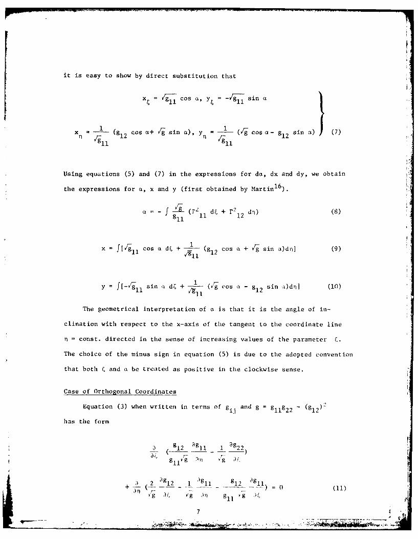
it is easy to show by direct substitution that

X = r Cos a, y= sin a IcIa+= 1i 7

x r (g12 Cos a+ g sin a), Y (cg Cos a- g1 2 sin a) (7)

Using equations (5) and (7) in the expressions for da, dx and dy, we obtain

the expressions for a, x and y (first obtained by Martini).

a = - C Wg (r2 1 1 d + r2 12 dn) (8)

PT- 1x = Wgll cos a dC + - (g12 cos a + vg sin a)dn] (9)

y = [-,gl1 sin a d + (vg cos a - g12 sin a)dn] (10)

The geometrical interpretation of a is that it is the angle of in-

clination with respect to the x-axis of the tangent to the coordinate line

c const. directed in the sense of increasing values of the parameter 6.

The choice of the minus sign in equation (5) is due to the adopted convention

that both C and a be treated as positive in the clockwise sense.

Case of Orthogonal Coordinates

Equation (3) when written in terms of gij and g = gllg 2 2 -(g12)

has the form

i g12 gl 1 3g22)

~ 1 2 g11 _1 __

+ (2 g12 1 ')g11 _ g1 2 11) 1 0 (11)

g , Vg )1) 9ivgl

7

which is an equation in three unknowns, viz., g11 , g1 2 and g2 2 " Here a

wide range of possibilities are open to express g1 2 and g22 as functions

of g11 either through algebraic or differential relations. Fortunately,

in the case of orthogonal coordinates this arbitrariness is minimal and

equation (11) can be reduced to a very simple form which can be solved

analytically. The following discussion and analysis pertains only to

orthogonal coordinates.

in the case of orthogonal coordinates, the coefficient g1 2 is zero,

i.e.,

912 = x x + Y yn 0 (12)

which is satisfied by the equations

x= -F Y,

yq Fx (13)

where F(x,y,t,n,x,,y,,x ,y ) > 0 is a continuous function of its arguments.

Let the boundary F 2 of a bounded region 2 in an Euclidean two-

dimensional space be a simple smooth curve x = x (c), y = y_( ), with a

uniformly turning tangent. In the region s?, let s2 be an annular subregions

bounded by the inner boundary F1 and the outer boundary F2 as shown in

Figure 1. The region ' is to be mapped onto a rectangular region R in thes

inj-plane by a transformation with the initial data

= x(~ ~0 < F

y~n) = y"(.) (14)

,so as to have

x = x(ECrI)

y =yCs,,,O (1.5)

8i4

where q and 71 are the actual parampfriL values associated with the

boundaries ['Ind 2' respectively, and x and y are periodic in the i-

argument with the period

2= (16)m

The set of equations (13) along with the initial data (14) can form a

well-posed initial-value problem for hyperbolic equations if certain

conditions on F are satisfied. It is to be noted that in this case no

boundary data is aeeded on the curve I' This problem has been considered

by StariusI0 .

Since in this paper the equation for the condition of an Euclidean

space (equation (11)) forms the basis of the proposed method, we expect

to have an elliptic boundary-value problem to be solved under the

Dirichlet conditions. Equation (11) with the substitution g12 0 and

on using equations (13) becomes

3 1 (F2gll)] + Fgll - = 0 (17)

Fgl 11

g22 = Fg g11

g = (Fg 1 1

Equation (17) can now be solved as an elliptic boundary-value problem

in gl provided that it can be proved that F is a function of E,,n and g11 .

These considerations on F will also provide a class of functions from which

F can be chosen in a simple wiy.

In Reference 10, Starius has proved the following properties of F:

(a) F is an invariant under translation and rotation of the coordinate

axes (x,y). Therefore, if (x,y) is a solution of equations (13), then it

9

.. .. ... .._ _. . .. ... .....__ _

can be shown that

= a + x cos 6- y sin e

y =b + x sin 6 + y cos 0

is a solution of the equations

: yiS Fy

where a,b and e are arbitrary constants. These considerations show that F

is not an explicit function of x and y.

(b) On the basis of the results obtained in (a), we have

F(F,, x,, x, y x Y ) = F(C,, x V, y V, x , y )

hence = for all values of e including 0 = 0. Evaluatingde

d F( ) , we obtain

= 0

F + F 3F + F-y y _L_ + x - = 09 Y rl 3x TI aY

This equation shows that F = F(Cn, g11 ' g2 2 ), so that F depends on

x XP , y Yr) through g11 and g2 2 only.

(c) The considerations in (a) and (b) along with equation (18) show that

g22 = g F2( ' r ' gill 922 )

so that in principle g22 can be expressed as a function of g1 l and con-

sequently F = F(F,,n, g1l). This proves the contention that in the case

of orthogonal coordinates, equation (17) is sufficient for the calculation

of gll"

The set of functions F > 0 satisfying the conditions (a), (b), and

(c) enumerated above also contain F = 1 as an element. This choice of r*

*This is by no means a restriction, as is demonstrated later.

10

77*0

yields the simplest possible form of the generating equation. With F = 1,

equation (17) becomes

32 p + h2 0 (19)

3 2 3r12

where

P = £n g11 ' g22 = g1l' V 2

= 0"* (20)

The boundary conditions are

P= P at On =0

=P(F) at rinn (21)

where the subscripts g and denote the inner and outer boundaries

respectively. The periodicity requirement is that

P( ,r) = P(& + 2k, rY) (22)

where

m

A general analytic solution of equation (19) under the conditions (21)

and (22) is

nnEn niP(4,n) = a + nK + E sinh - (n -r)(a cos n + b sin )/sinh

o n=ln n

noo (c rf n Ti (23

+ E= sinh (c cos + d sin -)/sinh (n12 n 2. n 2.(3

where

K = (co-a) (24)

TThere is no loss of generality in setting the parametric value i= 0. The

value n. must be interpreted as the difference between the actual values atthe outer and inner boundaries. The determination of rlis of crucialimportance to this work and is discussed in the next section.**Refer to the next section.

.. y~ . , , .. ,*mmo w

and

2Z 2Z

a= f ( )d c =1 P ()]o 22 o P ' 0 2Z o

a 2Z. co f7 2~! siZl= f os d' b f P )sin () -C dC (25)

f p. 2 C nT 2 n,

c = f P( ) cos T dC, d = oP ( sin dn 0 s -

Having determined the coefficients an, b, C and d as defined in (25),

we can obtain the values of gll from (23) for all values of and 9. To

find the expression for a we consider equations (5), which for orthogonal

coordinates are

1 3gll 1 3922

2/g 2 g

For g2 2 = g1 1 ' these equations become

1 9P 1 aP

C9 = 2 . (26)-''T 2 DC'

and on integration yield the exact expression for a.

cosh -O)= a(,o) + a cos a n -- TVH

n-l n i no2 sinh 2

cosh n~z'

+ (cn sin T-j d cos

2 sinhni

n 77 r1

cosh k-

-- (b cos - a sin-)n iTri n 2 n2 sinh

2 nJ (c sin T - d cos (27)

f ~l2 sinh--

Since the line integrals for the determination of x and y (cf. Eqs. (9)

and (1O))are independent of the path,vlz.,

12

(gll cos a) = (L sin a)

(gl sin a) = - 'g22 cos a)

hence

x(Cn) = x(,o) + J 0gg 2 2 sin a dn (28)

y(Cn) = y( ,o) + fo Fg22cos a dn (29)

The preceding analysis completes the basic development of the subject.

Coordinate Re-Distribution (Contraction)

In order to have the capability of re-distributing the coordinate lines

so as to have a control on the mesh spacings in the desired regions, we

consider a transformation from (4,n) to new coordinates ( ,n). The trans-

formation functions can arbitrarily be selected, but can also be linked in

some manner to the physical field behaviors. For example, in viscous

flow problems the effect of viscosity near a wall can be incorporated in

the transformation functions. Below we proceed without specifying these

functions and then give one example in the section on numerical method.

On transformation from (&,n) to (Tq), the covariant metric coefficients

transform as

axk x Z

gij = gkZ iax axi

so that on using the relation g22 = g1l and g1 2 = 0, we have

g = [ ) + (1-1)11g

92= [ ) + (-1lg 1 (30)

13

Ad L1

We now introduce the transformation

- f(r6) (31)

where the functions 0 and f are continuously differentiable and satisfy the

conditions

€(Eo) = 0, f(n.) - 0

where , 0 and ri 0 correspond respectively to t, and ) Defining

0

f d (31a)

dt, dti

we have from (30)

gl (11 ,-g l (1 (32b)

22 = i1

To obtain the solution in the (i,,) coordinate system, we merely have

to replace C and n by the functions p(,) and ( ) respectively in (23) and

(27), while (28) and (29) become

X(-,-) X(',7"7) + [ g22" sin O(r)dTi (33a)- 922

y( , ) 0 (,, ) + fn ,22 COS Al( I Odti (33b)

It must be noted that on transformation the resulting metric coefficients

911 and 22 are not equal.

The salient feature of the preceding analysis is that the solution

under the condition g 22 = gl11 can be used to obtain the solution for the

case 22 # gll by coordinate transformation.

14

Uniqueness Condition on t, for Orthogonal Coordinates

Any method for the generation of orthogonal coordinates on the preceding

lines has to be supplemented with a uniqueness condition on the behavior

of 7 and a method for its selection. The following analysis, besides

covering the above two aspects, also provides a general basis for the

earlier choice F - 1.

For the case of orthogonal coordinates, equations (7) call also be

expressed in the inverse form as

cos t - = -sin ,/ -

X ' V

Writing F = /g l, eliminating t between the above equations and then

bv cross differentiation, we obtain the following equations:

F) + ( F) 0 (34)") x x v I Fy

~(35)Ax (Fl', ) + i (F, ) = 0

I 6

Following Protter and Tutt I wo assume that the -.-curves in the xv-plane

are free trom sources and sinks. This condition establishes a uniqtte

correspondence between the points on each pair of constant

1 Iles. n tILhe absence of sources or sinks, we have

divIgrad ,' ) ( (36)

where ,(,j) is an arbitrary different lable unct ion of ,i, and as stch grad

"0(') Is oriented along the normal to the curve = coast. Using tihe

expressIons

grad ni g , I i 1)1g

15

_9h

in (36), we obtain

(n Vgll/g 2 2) =- / P/drn2 dn

Writing d l/v(n) and denoting the arbitrary function due to Integration

as inw(&), we obtain the result

V01) (37)= F= aQ) v(ri)

Introducing new variables

=fp(, f (38)

and using (37) in (34) and (35), we get

v-F " = 0 (39)

V' , = 0 (40)

Further using (37) and (38) in the fundamental equation (17), we obtain

+ _p- = 0 (41)

where

P"= E'ng l

= x,.. + y"., .. +

The solution of equation (41) is of the same form as that 01 equation

(19), viz., (23), and is obtained by replacing I. and tn by L," and t)' .

However, the important result obtai ned here is that a generating equation

of the form (19) or (41) must be supplemented with a Laplace equation for

or F.' respectively. This is the result or the required uniqueness

condition on :, for the generation of orthogonal coodinates. The condition

16

w, .

on V', i.e., equation (40), is implicitly satisfied by the coupled system

of equations (39) and (41) and needs no discussion.

The condition equation V2 = 0 can rigorously be satisfied in all

cases if we take as the angle traced out in a clockwise sense by the

common radius of the concentric circles in a conformal representation of

the inner and outer boundaries. The numerical scheme for this aspect of

the problem is an iterative one. In place of this elaborate scheme we haveI :

devised another method which is much simpler and non-iterative. Both

of these methods have been discussed in the next section.

17

Numerical Method of Solution

Based on tie formulation of the problem as discussed in the preceeding

sections, we now have a non-iterative algebraic computational problem

which can be handled in a straight forward manner. However, before solving

a specific problem, It is important first to establish an orthogonal

correspondence between unique points of the inner and outer boundary

curves which are to be connected by a specified number of C, = constant

curves, and second to obtain the numerical value of the parametric

difterence ii• Two methods for the establishment of x(4) and y(',)

are given below.

Met hod 1: It has been mentioned in equation (20) and later discussed

in the preceeding section that the curves constant in the physical xy-

plane must satisfy the Laplace equation V = 0. For this condition to

be satisfied wt can take a as the angle t ractd out in the clockwise sense

by tihe common radius of the concentri c circles in a conformal representation

of the inner and outer boundary curves as follows.

The tonction z = (z*), which conormally maps Lhe region of the z-

plane exterior to the specified curve C onto the region of the z'-plane

exterior to the circle C" o radius a , can be represented by a Laurent's

expansion as

= "+ p + i + ( + "i )1 + i)I (42)

For points ol tLie circ'unlference tit the circlt C

-i.

18

e

so that

x( p) = P + (p+a) cos i- q , sin + E (pn cos n & - n sin n ) (43)

n. 2

Y( =0 + (Pl - a ) sin C+ ql cos C + Z (pn sin n& + q cos n&) (44)n=2

The same form of equations can be written for the outer boundary with

A as the radius of the circle in the conformal plane.

Now y = y(x) is known either in functional or tabular form. Thus

starting from an initial guess for x the corresponding ordinates are used

to determine the Fourier coefficients from equation (44) which in turn

determine a new set of abscissae and then the ordinates, and so on. The

convergence of this iterative method yields x = x( ) and y = y() both

for the inner and outer boundaries. Note that after the completion of

convergence we have

fo [xoj() cos - y ( ) sin t]d (4 5a)

and

A = i f IxQ(,) cos ; - Y () sin tildl (45b)2r45bo

Method II: In lieu of using Method I, we have obtained equally good

results by proceeding as follows. This method looks to be equivalent to Method I.

The inner and outer boundary data is available to us either in tabular

or functional form as

y = Y(x), y, = y(x ) (46)

We now circumscribe circles around the inner and outer boundary curves. Two

cases arise depending on whether the circles are concentric or nonconcentric.

Case I: If the circumscribed circles are concentric (Fig. 2a), then

we select those sets of ordinates which correspond to the abscissae

19

= r cos 4and x.= rL cos 4 where r and rL are the radii of theS LS L

circumscribed circles.

Case 11: If the circumscribed circles are non-concentric (Fig. 2b),

then we first use the formula for the conformal transformation of non-

concentric to concentric circles (Kober) 17and choose the abscissae by

using the following equation.

x(S)= [1 -c'Y Cos 4)ix (1- c'Y Cos 4)+ c y ~ sin4LL

+ r (c cos ~p-ycos(C

- cy Sill -j L cy Cos )-cy x L sin

- r L (c sin 4) + y sin(4

/(l - 2 cy cos 4+ c 2 2 ) (47)

where

r rs radii of outer and inner circumscribed circles.

(xLL and (x,,y) coordinates of the centers.

=2 (x -x ) + (y -ys L s L

p= -tail- 1 (S )x -_x

c= (d- + r - r") + I (d + r - r)- -4d r2 I } 12 /2drL s L1 s L L

t =cr 1

y = I for the outer boundary.

rL d -tY r ------ for the inner bouindary

The ordinates are now selected corresponding to tthe set of abscissae

given by (47).

20

Determination of n

The parametric difference n. is connected in some manner with the

"modulus" of the domain. Determination of the modulus for annular regions

18 19has been considered by Burbea and Gaier . In this paper we base the

determination of n on the radii a and A in the conformal representation

process described in equations (45), and define it as

n A) (48)a

If 'Method I is used then A and a are available as parts of the converged

iteration, while if Method II is used, then they are obtained by simple

quadratures applied to equation (45).

Having determined the appropriate x( ) and y( ) both for the inner

and outer boundaries, we first calculate the values of (g1 l)6 and (g 11

numerically and then of P (E) and P.(). Based on these distributions

the Fourier coefficients a , b , c and d are computed by numericalnn n n

quadrature through the use of equation (25). Since these values of the

coefficients are independent of the spacings between n = constant lines

the same values are used when a redistribution of n = constant lines is

desired. Substituting the Fourier coefficients in equation (23) we

determine the values of P(',) and hence of g11 (i,n) for the whole

annular region. A knowledge of P( ,,n) determines a(j,,) through equation

(27) and so also the Cartesian coordinates x(Q,q) and y(i,n) through

equations (28) and (29) by numerical quadrature.

A computer program with the option of redistributing the coordinate

lines in any desired manner has been written and used to generate the

orthogonal coordinates for various annular regions as shown in Figures 3-8.

21

For the example problems we have chosen the following forms of the function

(p and f of equations (31).

0

-C-

K]

f(2) - ° (49)nl-n ~ '--)

so that2 TI K)

=+ = T [ - ) Zn K ]

m&M0 1) (50)

where K > 1 is an arbitrary constant, Z = 1, and 4 = T= correspond

respectively to 4 = 2Z = 27T and n = r. We treat 4 and n as integers so

that Zm 1, = IMAX, 1 1, n = JI4AX. Since ro is known from (48),

hence by specifying the numerical values to K and JMAX we can create the

desired mesh control in the direction of n. The value of K between 1.05

and 1.1 is quite sufficient20 to have very fine grid spacing near the

inner boundary.

The number of terms to be retained in the series (23) is usually small

for convex inner and outer boundary curves, though we have retained (MIAX-I)

number of coefficients in each computation. This number is the optimum

21number of terms in a discrete Fourier series having IMAX number of points

in one period. The average computer time for the complete computation on

the UNIVAC 1100/80 for IMAX = 73 and JMAX = 60 field is about 2.75 minutes.

22

Summary of Numerical Experimentations

In the course of this investigation a number of cases of inner and

outer boundary shapes and orientations have been tested through the

developed computer program. The main conclusions are listed below:

(i) The method works very effectively for smooth and convex

boundaries of any shape and orientation (cf. Figures (3)-(5) and

(7)).

(ii) For concave boundaries a method similar to that of Eiseman

1 3

has to be used in the placement of the outer boundary to avoid

intersecting = constant lines (cf. Fig. 8).

(iii) Sharp turns or corners are not admissible and have to be rounded

to avoid singularities (cf. Fig. 6).

23

i! 24.

' i I1|| I * .4. --

Comparison with the TTM Method

As discussed in the introduction, the choice of the proposed method

has been motivated by two considerations: (i) to choose a set of equations

which are fundamental to the intrinsic nature of the space in which the

coordinates are sought, and (ii) to minimize the inherent arbitrariness

in the selection of relations among the metric coefficients. It is the

purpose of this section to show that for the case of orthogonal coordinates

the equations of TTM (Ref. 7,20) can be reduced in a simple form which can

also be used to achieve the above two stated purposes.

The two-dimensional Laplacian of a scalar of general coordinates C and

n is

v2- 1g 22 1 2 P n) -1 92S () + )] (51)

Introducing the operator

= g2 2 a -2 g12 an + g11 n (52)

in (51) gives another form

v 2 p D2 + V2+ i V2 (53)

g fn

Writing y = x and then 0 = y in (53), we recover the equation of TTM,

which are

D2x = -g(x V2 + x V 2n) 'i

D2y = -g(y V2, + ynV 2 rn) (54)

For orthogonal coordinates g12 = 0, so that

+ g1 = -2(x V2E + x V2 r)g22x,, 11 glxn n

+ glY = V + y V2 n) (55)

24

Also, for orthogonal coordinates, equation (51) gives

12 )3 ("rg 2 2 /gll )

gllg 2 2

v1, (-g 11 /g 2 2 ) (56)

11 i22

It is immediately concluded from equations (56), that if the generating

system is taken to be

VF% = 0, V'n = 0

then gl1 /g2 2 = K = constant. The choice K = 1 gives the condition for the

Cauchy-Riemann equations. A change of variable such as n' = n/K

achieves the same purpose. In any event, without loss of generality,

equations (55) take the form

y + v 0 (57)

It will now be shown that even when the generating system is taken as

V:1, = -f (itl), = -f2(i.,r,)

f and f? being arbitrary functions, the equations of the form (57) are

again obtained.

Following the results of previous section, that, in the absence of sources

or sinks in either the i, or tj lines, the most general form of g 11/g 2 2 is

where o' and v are arbitrary differentiable functions. Using (56) in (55)

and defining new variables

JiiG'd"i., = f (58)

25

41-

we obtain

r1 ) 0)

Y- + Y ' " =0 (59)

where

v2C" = O, V211 = 0

From the foregoing analysis we conclude that the set of equations (59) are

quite general and capable of generating orthogonal coordinates (as has

earlier been proposed by Pope 9),and there is no need to solve a more

difficult and time consuming set of non-linear equations (55). Further

the method of solving equations (59) follows the same patterns as that of

the proposed method of this paper as discussed before.

26

I

' 26

3;€

Conclusions

A new method for the generation of orthogonal coordinates in two-

dimensional regions has been proposed. The method shows that much of the

arbitrariness in the choice of relations among the metrical coefficients

can be minimized by the use of the condition of an Euclidean space. The

method can also be used for simply connected regions only by obtaining the

solution of the linear equation (19) under the changed boundary conditions.

Besides, the proposed method can also be extended to three-dimensional

regions.

Acknowledgement

This research has been supported in part by the Air Force Office of

ocientific Research, under Grant

27

Al

Vt

ReferencesI.

1. A. J. Winslow, "Numerical Solution of the Quasi-Linear Equation in aNon-Uniform Triangular Mesh", Journal of Computational Physics, 2,

149 (1966).

2. W. D. Barfield, "An Optimal Mesh Generator for Lagrangian Hydrodynamic

Calculations in Two Space Dimensions", Journal of Computational Physics,6, 417 (1970).

3. W. H. Chu, "Development of a General Finite Difference Approximation

for a General Domain, Part I: Machine Transformation", Journal of

Computational Physics, 8, 392 (1971).

4. S. K. Godunov and G. P. Prokopov, "The Use of Moving Meshes in GasDynamics Computations", USSR Computational Mathematics and Mathematical

Physics, 12, 182 (1972).

5. A. A. Amsden and C. W. Hirt, "A Simple Scheme for Generating General

Curvilinear Grids", Journal of Computational Physics, 11, 348 (1973).

6. D. E. Potter and G. H. Tuttle, "The Construction of Discrete Orthogonal

Coordinates", Journal of Computational Physics, 13, 483 (1973).

7. J. F. Thompson, F. C. Thames, and C. W. Mastin, "Automatic Numerical

Generation of Body-Fitted Curvilinear Coordinate System for Field

Containing any Number of Arbitrary Two-Dimensional Bodies", Journal of

Computational Physics, 15, 299 (1974).

8. J. F. Thompson, F. C. Thames, and C. W. Mastin, "'TOMCAT'-A Code for

Numerical Generation of Boundary-Fitted Curvilinear Coordinate Systemon Fields Containing any Number of Arbitrary Two-Dimensional Bodies",

Journal of Computational Physics, 24, 274 (1977).

9. S. B. Pope, "The Calculation of Turbulent Recirculating Flows in

General Orthogonal Coordinates", Journal of Computational Physics,26, 197 (1978).

10. G. Starius, "Constructing Orthogonal Curvilinear Meshes by Solving

Initial-Value Problem", Numerische Mathematik, 28, 25 (1977).

11. J. F. Middlecoff and P. D. Thomas, "Direct Control of the Grid Point

Distribution in Meshes Generated by Elliptic Equations", AIAA

Computational Fluid Dynamics Conference, Paper No. 79-1462 (1979).

12. C. D. Mobley and R. J. Stewart, "On the Numerical Generation ofBoundary-Fitted Orthogonal Curvilinear Coordinate Systems", Journal

of Computational Physics, 34, 124 (1980).

28

13. P. R. Eiseman, "A Coordinate System for a Viscous Transonic CascadeAnalysis", Journal of Computational Physics, 26, 307 (1978).

14. R. T. Davis, "Numerical Methods for Coordinate Generation Based on

Schwarz-Christoffel Transformation", AIAA Computational Fluid DynamicsConference, Paper No. 79-1463 (1979).

15. L. P. Eisenhart, "Riemannian Geometry", Princeton University Press(1926).

16. M. H. Martin, "The Flow of a Viscous Fluid, I", Archiv of RationalMechanics and Analysis, 41, 266 (1971).

17. H. Kober, "Dictionary of Conformal Representations", Dover Publications,

Inc. (1952).

18. J. Burbea, "A Numerical Determination of the Modulus of DoublyConnected Domains by Using the Bergman Curvature", Mathematicsof Computation, 25, 743 (1971).

19. D. Gaier, "Determination of Conformal Modulus of Ring Domains andQuadrilaterals", In-Lecture Notes in Mathematics, No. 399, Springer-Verlag, Berlin (1974).

20. Z. U. A. Warsi and J. F. Thompson, "Machine Solutions of PartialDifferential Equations in the Numerically Generated CoordinateSystems", Engineering and Experimental Research Station, MississippiState University, Rep. No. MSSU-EIRS-ASE-77-1, August (1976).

21. F. B. Hildebrand, "Introduction to Numerical Analysis", McGraw-Hill

Book Company, Inc., (1956).

29

rI

rr

r 3

Y

x

2

n= n.

r Ir

----TIM 1I

r I.r*

Transformed Plane

(Natural Coordinates)

Figure 1. Physical and Transformed Planes.

30-- . . .. , _

I2

(a)

Figure 2. (a) Concentric circumscribed circles C1 and C2 of radii rs, r Lrespectively with center at the origin. (b) Non-concentriccircumscribed circles C, and C 2 of radii r and r Land centersat z aand z L respectively.s L

31

Figure 3. Confocal ellipses. Semi-major axes 1.48, 5.0, and semi-minor

axes 0.5, 4.802 respectively. Only 38 n = const. lines shown

for detail.

32V O W -

Figure 3. Confocal ellipses. Semi-major axes 1.48, 5.0, and semi-minoraxes 0.5, 4.802 respectively. only 38 r, cotist. lines sh~ownfor detail.

32

Figure 4. A blunt body section with elliptical outer boundary.

33

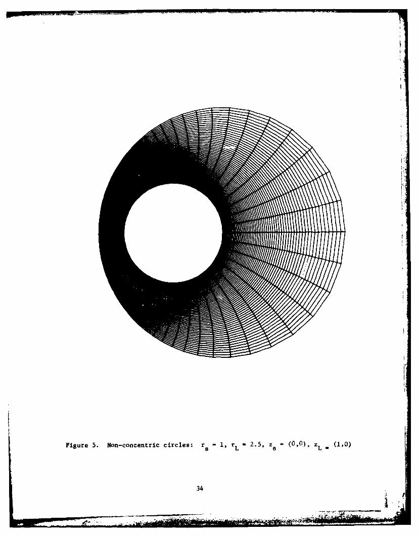
Figure 5. Non-concentric circles: r. 1, r L -2.5, z.- (0,0), ZL (1PO)

34

Figure 6. Joukowsky's airfoil with slightly rounded trailing edge.

35 .

Figure 7. Non-concentric ellipses. Size data same as in Figure 3.z = (0,0), z L (1,).

36

to 0)

.0O u

>4

:3 4,-4Ui0

100

0 u u

37coc

M 04T'5R