658 IEEE JOURNAL OF SELECTED TOPICS IN ... - asl… · 658 IEEE JOURNAL OF SELECTED TOPICS IN...

658 IEEE JOURNAL OF SELECTED TOPICS IN SIGNAL PROCESSING, VOL. 2, NO. 5, OCTOBER 2008

Carrier Recovery Enhancement for Maximum-Likelihood Doppler Shift Estimation in

Mars Exploration MissionsFederico S. Cattivelli, Student Member, IEEE, Polly Estabrook, Edgar H. Satorius, Member, IEEE, and

Ali H. Sayed, Fellow, IEEE

Abstract—One of the most crucial stages of the Mars ExplorationMissions is the Entry, Descent, and Landing (EDL) phase. DuringEDL, maintaining reliable communication from the spacecraft toEarth is extremely important for the success of future missions, es-pecially in case of mission failure. EDL is characterized by verydeep accelerations, caused by friction, parachute deployment androcket firing among others. These dynamics cause a severe Dopplershift on the carrier communications link to Earth. Methods havebeen proposed to estimate the Doppler shift based on MaximumLikelihood. So far these methods have proved successful, but itis expected that the next Mars mission, known as the Mars Sci-ence Laboratory, will suffer from higher dynamics and lower SNR.Thus, improving the existing estimation methods becomes a neces-sity. We propose a Maximum Likelihood approach that takes intoaccount the power in the data tones to enhance carrier recovery,and improve the estimation performance by up to 3 dB. Simula-tions are performed using real data obtained during the EDL stageof the Mars Exploration Rover B (MERB) mission.

Index Terms—Doppler effect, frequency estimation, maximum-likelihood estimation, space vehicle communication.

I. INTRODUCTION

N ASA’S Viking missions made history when they becamethe first spacecraft to land safely on Mars in 1976.

The next landing was accomplished twenty years later by the1996 Pathfinder mission, which introduced innovative landingtechniques. The two Mars Exploration Rover (MER) missionsnamed MERA and MERB were launched by NASA in mid2003, landing the rovers on Mars on January 2004. These rovershave travelled for miles across the Martian surface, conductingfield geology and making atmospheric observations.

NASA’s next mission requiring safe landing on the surfaceof Mars is known as the Mars Science Laboratory (MSL), andis planned for the Mars launch opportunity in 2009. The pri-mary objective is to investigate the habitability of Mars (i.e.,

Manuscript received November 01, 2007; revised July 21, 2008. Current ver-sion published December 10, 2008. This work was supported by a Grant fromthe Jet Propulsion Laboratory under award 1276256 and by National ScienceFoundation (NSF) awards ECS-0601266 and ECS-0725441. The associate ed-itor coordinating the review of this manuscript and approving it for publicationwas Prof. Alle-Jan van der Veen.

F. S. Cattivelli and A. H. Sayed are with the Department of ElectricalEngineering, University of California, Los Angeles, CA 90095 USA (e-mail:[email protected]; [email protected]).

P. Estabrook and E. H. Satorius are with the Jet Propulsion Laboratory,Pasadena, CA 91109 USA (e-mail: [email protected]; [email protected]).

Digital Object Identifier 10.1109/JSTSP.2008.2005289

Fig. 1. Entry, Descent, and Landing stages during MER missions (from [5]).

its capacity to sustain life) [1]. One of the most outstandingcharacteristics of MSL compared to previous Mars Explorationmissions is the advanced landing techniques that will be em-ployed. The Mars Entry, Descent, and Landing (EDL) stagesof the MSL mission will deliver a larger rover to a higher alti-tude, while maintaining precision landing [2], providing accessto previously unaccessible sites [2]–[4].

A. Entry, Descent and Landing

The EDL stages of the mission refer to those stages betweenthe point when the shuttle enters the atmosphere of Mars andwhen it finally lands on its surface. Fig. 1 shows the EDL stagesfor the 2004 Mars Exploration Missions [6], [5].

During EDL, it is highly important to maintain communica-tion between the spacecraft and Earth, since the information sentcould be critical for the success of future missions, especiallyin the eventuality of a mission failure. Before Entry and untilthe lander is separated from the backshell, communication is bya direct-to-Earth (DTE) X-band (8.4 GHz) link. After separa-tion the backshell antenna can no longer be used, and commu-nication is achieved using two links: a main UHF relay link tothe Mars Odyssey or Mars Global Surveyor spacecraft, and abackup DTE link using the rover antenna. The DTE link uses aspecial form of MFSK modulation that transmits one out of 256possible data tones every 10 s. This form of modulation will bediscussed in the next section.

EDL is the most challenging phase of the spacecraft to groundcommunications [6]. There exist several phenomena that con-tinuously accelerate and decelerate the spaceship during EDL,such as atmospheric friction and parachute deployment duringEntry, bridle descent, swinging on bridle, rocket firing and bridle

1932-4553/$25.00 © 2008 IEEE

Authorized licensed use limited to: Univ of Calif Los Angeles. Downloaded on January 21, 2009 at 13:38 from IEEE Xplore. Restrictions apply.

CATTIVELLI et al.: CARRIER RECOVERY ENHANCEMENT FOR ML DOPPLER SHIFT ESTIMATION 659

Fig. 2. Frequency profile of MERA during EDL.

separation during Descent, and bouncing on the Landing stage.All these factors contribute to the effect known as Doppler shift,where the frequency of the main carrier of the communica-tions signal is shifted from its nominal value. Fig. 2 shows theresidual frequency profile observed during the EDL stage of theMERB mission. It can clearly be observed that the Doppler shiftranges between 3 and 6 kHz. This range refers to the frequencyresidual which results after a first stage of Doppler shift correc-tion; the actual Doppler shift has a range of about 90 kHz (see[5] for example). The Doppler rate, defined as the derivative ofthe Doppler shift, ranges between 200 and 200 Hz/s, exceptduring parachute deployment where it can reach 1000 Hz/s.

For the 2009 Mars Science Laboratory mission, both higherDoppler shifts and Doppler rates are expected This is due to thelanding techniques of the new mission, which requires landing aload of about 1000 kg, nearly twice as that of the MER missionsand with a tighter landing ellipse. Predicted Doppler shifts forthe MSL mission range within 15 kHz, and predicted Dopplerrates are in the range 600 to 300 Hz/s. Also, since the shuttlewill be able to land in areas farther away, a lower SNR is ex-pected (possibly 0.5 to 3 dB lower).

B. Doppler Shift Estimation

In order to recover the data transmitted by the spacecraftduring EDL, it is necessary to estimate and correct the Dopplershift of the carrier. Several frequency estimation techniqueshave been proposed for such purposes. Maximum-likelihoodestimation of a single tone embedded in noise is discussed in[7] and [8]. Estimation of signals where the tone frequencychanges linearly with time has been studied in the context ofchirp signals (see, for example, [9]–[16]). The case where thenoise is not additive Gaussian has also been considered in [17]and [18]. In [19], an adaptive algorithm is proposed to track thecarrier frequency once it has been acquired. Frequency trackingis also considered in [20]. For the Mars Exploration missions,the technique used is Maximum Likelihood both for carrieracquisition and tracking [5].

In this paper we focus on Maximum Likelihood estimationof the Doppler shift. We address the problem of carrier acquisi-tion, where we need to coarsely estimate the received carrier fre-quency over a wide bandwidth. We show that improvement overprevious methods can be obtained by exploiting (rather than ig-noring) the power in the data tones of the transmitted signal toaid the carrier acquisition process. It is shown that the methodcan provide between 1 and 3 dB improvement, and is suitablefor low data-rate, low SNR, and highly dynamic communicationsystems such as the one used in the Mars exploration missions.

II. SIGNAL MODEL

We now review the communications system used for the MERmissions. As mentioned before, the DTE link uses a special formof MFSK modulation with 8 bits transmitted every 10 s. Themodels for the transmitted and received signals are describednext.

A. Transmitted Signal Model

The signal transmitted from the spacecraft to Earth during theEDL phase has the following form [5]:

where• is the transmitted signal power;• is the nominal carrier frequency;• is the modulation index (typically, );• is the limiting function defined by

• is the data tone frequency; it assumes one out of 256possible values transmitted every 10 s;

• is the time instant where transmission began (typically,).

B. Received Signal Model

The signal received on Earth during EDL has the followingmodel [5]:

(1)

where• is the time-varying received signal power;• is the time-varying carrier frequency, which is mod-

eled as



where is the unknown Doppler frequency shift;• is a realization of an zero-mean, additive white

Gaussian noise wide sense-stationary process with vari-ance .

The signal is a bandpass signal centered around the fre-quency . It can be expressed in the form

where is the lowpass equivalent of ,and and are its in-phase and quadrature components.The same relation holds for , namely

The signal is the low-pass equivalent of , cor-responding to a realization of a complex, zero-mean, ad-ditive white circular Gaussian noise process of the form

, with and independenthaving variance . Note that the variance of is .The low-pass equivalent of (1) is therefore

with .We can express the signal in discrete-time by sampling

at the rate , and using the compact notation

and . Then

(2)

where we defined

(3)

Note that if we assume that the data tone frequency is con-stant between two arbitrary time instants and

, we have

where is an unknown phase.Throughout this work, the measure that will be used to quan-

tify the noise level in a signal is the signal-to-noise-PSD ratio[5], and will be denoted by SNR. This measure is defined as theratio of the received signal power to the white noise power spec-tral density in dB. Given a noise power spectral density of ,the SNR is defined as

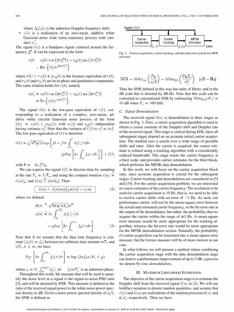
Fig. 3. Carrier acquisition, carrier tracking, and data detection system for MERmissions.

Thus the SNR defined in this way has units of Hertz, and in thedB scale this is denoted by dB-Hz. Note that this scale can beconverted to conventional SNR by subtracting

dB when kHz.

C. Signal Demodulation

The received signal is demodulated in three stages asshown in Fig. 3. First, a carrier acquisition algorithm is used toobtain a coarse estimate of the Doppler shift and Doppler rateof the received signal. This stage is critical during EDL since allsubsequent stages depend on an accurate initial carrier acquisi-tion. The method uses a search over a wide range of possibleshifts and rates. After the carrier is acquired, the coarse esti-mate is refined using a tracking algorithm with a considerablyreduced bandwidth. This stage tracks the carrier frequency ata finer scale, and provides carrier estimates for the third block,which performs the MFSK data demodulation.

In this work, we will focus on the carrier acquisition blockonly, since accurate acquisition is crucial for the subsequentstages. Carrier tracking and demodulation are considered in [5]and [19]. For the carrier acquisition problem, we are interestedin coarse estimates of the carrier frequency. The resolution to beused for carrier acquisition is 10 Hz, that is, we need to be ableto resolve carrier shifts with an error of Hz. As such, ourperformance metric will not be the mean-square error betweenthe actual and estimated carrier frequency, or the bit error rate atthe output of the demodulator, but rather, the probability that weacquire the carrier within the range of Hz. A mean-squareerror measure would be more appropriate for the tracking al-gorithm, whereas the bit-error rate would be more appropriatefor the MFSK demodulation section. Naturally, the probabilityof carrier acquisition can be translated into a mean-square errormeasure, but the former measure will be of more interest in ourcase.

In what follows we will present a method where combiningthe carrier acquisition stage with the data demodulation stagecan lead to a performance improvement of up to 3 dB, a processwe denote by tone demodulation.

III. MAXIMUM LIKELIHOOD ESTIMATION

The objective of the carrier acquisition stage is to estimate theDoppler shift from the received signal in (2). We will useboldface notation to denote random quantities, and assume that

and are realizations of the random processes and, respectively. Then we have



We start by introducing the following assumptions.• The noise process is complex, zero-mean, circular

Gaussian and iid, with variance .• The data is analyzed in segments of samples. Typ-

ical values are and kHz,leading to an analysis segment duration of second.During each segment, the Doppler shift and rate areassumed constant, and are modeled as unknown determin-istic parameters.

• The complex amplitude is modeled as a piecewiseconstant deterministic parameter, i.e., is assumedconstant in intervals of duration samples, and the ampli-tude corresponding to the th segment is denoted by .This assumption is useful to account for multiplicativenoise and channel fading, since it allows more frequentchanges in the amplitude, compared to less frequentchanges in Doppler shift and rate. Furthermore, in order toguarantee an average signal power of for the low-passequivalent (2), we require:

(4)

Let and denote the random vectors of length NM withindividual entries and , respectively.Under these assumptions, the probability density function (pdf)of the signal is

By taking the logarithm we arrive at the following log-likelihoodfunction:

The Maximum-Likelihood (ML) criterion estimates andby maximizing the above log-likelihood function, which

is equivalent to minimizing the following quadratic form:

(5)

Differentiating the above cost with respect to , and settingthe result to zero, we get the optimal amplitudes

Substituting this result into (5) we obtain that the original Max-imum-Likelihood problem is equivalent to the following maxi-mization problem:

(6)

The solution to problem (6) will depend on how we model theunknown phase . In general, will be some function ofthe Doppler frequency shift . This shift can be describedusing a Taylor series expansion, say

(7)

Thus, by restricting (7) to a few terms, problem (6) becomes afunction of a few optimization parameters, as is shown next.

A. Linear Frequency Model

We assume a linear profile for the Doppler shift, and firstignore data tones. The linear profile assumption is reasonablewhen the length of the data segment to be analyzed is short com-pared to the change in Doppler frequency. The Doppler shift ismodelled as

(8)

where the Doppler frequency and Doppler rate are un-known. Since we are ignoring the data tones, we set in(3) to obtain

where represents some constant phase which depends on .Then the maximization problem (6) becomes

(9)

This problem is also known as periodogram maximization, andis not convex in general. It is solved typically by searching overa predefined set of possible rates and frequencies , and thenfinding the combination that maximizes the expression. Thus, itinvolves a 2-D grid search, and the finer the grid, the larger thecomplexity of the search. The method can be extended from thelinear case to take into account higher order terms in the expan-sion (7). For instance, [21] suggests a second-order approxima-tion of the Doppler shift, which leads to a search over and

.It is important to note that and are continuous param-

eters, even though the grid search uses a set of discrete searchvalues. The finer the grid, the more likely it will be to find apoint close to the actual values.

In what follows we will refer to (9) as the ML method, sinceit is the one currently used in the MER missions. However, itshould be kept in mind that the method that follows is also Max-imum Likelihood, but with different modeling assumptions.

B. Linear Frequency Model With Data Tones

We now take into account the presence of the data tones in thefrequency model, and will show how the combined estimation



of the Doppler shift and the data tones leads to performanceimprovement. The Doppler shift is again assumed to be linearas in (8). When data tones are taken into account in the modelfor we obtain from (3)

(10)

Now the ML procedure (6) becomes

(11)

We will refer to (11) as the Maximum Likelihood with ToneDemodulation (MLTD) method. The algorithm typically oper-ates over segments of duration second

and kHz). Compared to the ML method (9)without considering data tones, MLTD is more complex becausewe also have to search over the phases and the data tone fre-quencies . However, as will be discussed later in this section,

comes from a discrete set, and in some cases may be knowna priori. Also, rough estimates of will be sufficient to provideperformance improvement.

C. Interpretation of the Tone Demodulation Process

The following interpretation shows why we should expect animprovement of about 3 dB when we take into account the datatones as in (11) over the earlier method (9) where data tones areignored. The interpretation is included to provide the reader withan intuitive explanation of the process. A more rigorous analysiswill be provided in the following section. We will assume, onlyin this section, that , the Doppler rate and thatthe amplitude is constant.

From (2) and (10), the received signal is of the form

(12)

with . Now note the following:

(13)

Consider the Fourier series expansion of the Sqr function:

(14)

where

Since for even, it can be observed that containstones at frequencies . The power of the

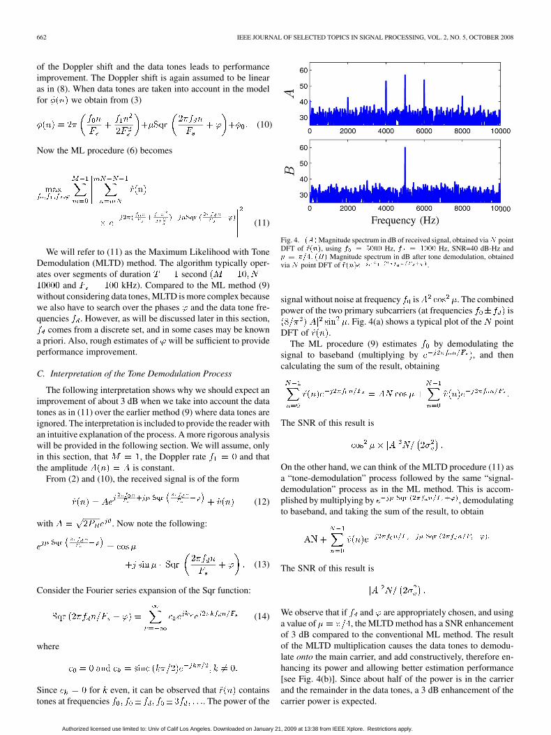
Fig. 4. ��Magnitude spectrum in dB of received signal, obtained via� pointDFT of ��, using � � �� Hz, � � �� Hz, SNR=40 dB-Hz and� � ��. �� Magnitude spectrum in dB after tone demodulation, obtainedvia � point DFT of �� .

signal without noise at frequency is . The combinedpower of the two primary subcarriers (at frequencies is

. Fig. 4(a) shows a typical plot of the pointDFT of .

The ML procedure (9) estimates by demodulating thesignal to baseband (multiplying by , and thencalculating the sum of the result, obtaining

The SNR of this result is

On the other hand, we can think of the MLTD procedure (11) asa “tone-demodulation” process followed by the same “signal-demodulation” process as in the ML method. This is accom-plished by multiplying by , demodulatingto baseband, and taking the sum of the result, to obtain

The SNR of this result is

We observe that if and are appropriately chosen, and usinga value of , the MLTD method has a SNR enhancementof 3 dB compared to the conventional ML method. The resultof the MLTD multiplication causes the data tones to demodu-late onto the main carrier, and add constructively, therefore en-hancing its power and allowing better estimation performance[see Fig. 4(b)]. Since about half of the power is in the carrierand the remainder in the data tones, a 3 dB enhancement of thecarrier power is expected.



D. Complexity of the Tone Demodulation Process

The ML method (9) requires a search over anddiscrete frequencies and , respectively, whereas the MLTDmethod (11) requires searching also over and dis-crete values of and , respectively. Using typical valuesof and

(see Section IV), MLTD requires on the order offloating point operations. More-

over, MLTD is roughly 1000 more complex than ML in itsgeneral form. However, when is known, MLTD is onlyeight times more complex than ML, and provides significantperformance improvement. In general is unknown, but sincethis frequency is kept constant for every 10 segments, the valuemay be known from a previous segment estimate. When isunknown, the method is still useful, since it can be applied onlyto those segments of the signal which are extremely noisy, andwhere the original ML method performs poorly.

Also, note that if we approximate (14) by its first harmonic

then we need not take a new DFT for every value of and, but rather replace them by shifts and additions of the same

spectrum. If we can do shifts and additions efficiently, we canreduce the complexity of MLTD to that of ML, at the expenseof some performance hit due to the above approximation.

IV. PERFORMANCE ANALYSIS

We now analyze the performance of the MLTD estimationmethod. The analysis can be extended to the case where theDoppler shift is assumed to include higher order terms of theexpansion (7). The following analysis extends the results of [5]to the more general case (11) when data tones are taken intoaccount rather than ignored.

A. Signal Model and Performance Metric

It is assumed that the received signal has the form (12), witha piecewise-constant amplitude as discussed in Section III, andthat the data tone frequency is fixed at . The signal is analyzedin segments of duration seconds, where . We usethe notation and to refer to the true parameters of thereceived signal. The MLTD method of (11) requires multiplying

by

where we have introduced the notation and to referto the dummy search variables, and where denotes a vector ofsearch parameters ordered as follows:

The ML estimates of and are found by solving

(15)

with

(16)

The cost is a realization of a real, scalar random vari-able whose distribution depends on the parameters

and . Once is received, we compute the deter-ministic cost , and the ML method selects the set of parametersthat maximize .

To make the analysis tractable, we introduce some simpli-fying assumptions. Define the auxiliary function

(17)

When the argument of is equal to a constant , we get

We assume that:• for some integer . This assumption is not

true in practice, since is a continuous variable. The far-ther is from a multiple of , the worse our esti-mate will be. However, since this problem will affect in thesame manner the proposed MLTD method and the originalML method, we will assume in our calculations that thisassumption holds. Typically, we will havesec, so will be considered a multiple of 10 Hz. Thus,the search will be performed at integer multiples of ,that is, for some integer . Since we arefree to choose the tone frequencies , we will also assume

for some integer• if , for any integer

. This result is also not true in general, but the approxima-tion is good for values large enough. As we decreasethe value of , the probability of making an error by se-lecting a grid point close to the true one increases, but sodoes the frequency resolution. Moreover, we are mostly in-terested in estimating the Doppler shift , since we assumea carrier tracking stage follows, which reduces the searchrange around the estimated frequency . Hence small er-rors in detecting are not of major concern as long asis acquired correctly.

The metric used to evaluate the performance of the algorithmis the probability of error in carrier acquisition, , defined asthe probability that the estimate is different from the truevalue . In terms of , it can be expressed as follows:

(18)

for at least one set of values of such that, and for every value of .

To derive expressions for , we will proceed as follows. Forevery combination of values of the parameters and ,we will derive an expression for the probability distribution ofthe resulting random variable . Subsequently, we will compute

from (18).



B. Statistics of the Estimates

Define the differences

. It then follows that

(19)

From (13), we have

(20)

We also introduce the following useful notation:

Using (19), (20), (17), and (14), we arrive at

(21)

Equation (21) is important for our analysis, since it allows us tofind an expression for statistics of for every value of searchparameters and as a function of the true parameters

and .

Note that is a zero-mean, complex Gaussian random vari-able with variance , independent of for . There-fore, we have that

where represents a noncentral chi-square distributionwith degrees of freedom and noncentrality parameter

(22)

The pdf of is (for )

(23)

where is the modified Bessel function of the first kind.When is distributed according to a central chi-squaredistribution. In this case, the pdf becomes (for )

(24)

C. Parameter Classes and Probability of Error

In our search procedure we will search overand discrete values of and , respectively. Let

denote the space of all possiblesearch vectors . We will partition this space as follows.

When is known, only partitions 0 to 3 exist. Whenever be-longs to or , the value of will be equal to the true value

. For every partition, we define a set of identically distributedrandom variables

Using (21) and (22), and using the relation, we obtain



Fig. 5. Probability of error in carrier acquisition vs. SNR for��

�. (Continuous line) ML method. (Dashed line) MLTD. (Dot-dashed line) 3-dBimprovement over ML method.

(25)

A more detailed derivation can be found in the Appendix. Wealso define

Thus, the probability of error can now be rewritten as

where the last approximation follows from the fact that the prob-ability of is high. We will evaluate in three sce-narios: when and are known, when only is known, andwhen all the parameters are unknown.

1) Known and : When and are known, the param-eter space is partitioned in four classes. Class has oneelement, classes and have two elements each, and class

has elements. Moreover, andare uncorrelated (and therefore also independent) wheneverand are in different classes. This means that the areindependent in and . Let and denote the probabilitydensity function and cumulative density function, respectively,of the random variable . Since all random variables arealso independent, we have that the probability of correct carrieracquisition is

(26)

Fig. 5 shows the probability of error in carrier acquisition,versus the SNR for the ML method without tone demodula-

tion (ML) and with tone demodulation (MLTD) using expres-sion (26) where and is known. We have chosen the

values and as in [5]. The curve forML is the same one reported in [5]. Also shown is a 3 dB-im-provement curve of ML. We can clearly see that MLTD achieves3-dB improvement for low values of SNR, and even better im-provement for high values of SNR. Though a 3-dB improvementis expected, more than that is surprising. The reason is that inthe ML curve, the performance at high values of SNR is lim-ited by the presence of the primary data tones at and

. When we apply tone demodulation, not only we doublethe power of the carrier at , obtaining a 3-dB improvement,but we also eliminate the data tones at frequencies and

(see Fig. 4). Thus, the improvement is larger than 3 dBfor high SNR. This is the most optimistic scenario, where and

are known. Though in practice we may have knowledge of, we will never know exactly what is. We will consider the

effect of these parameters next.2) Known : The maximization procedure (15) requires

searching over phases . We propose searching over a setof phases uniformly distributed between 0 and . Analyzingexactly the performance of this method is challenging, becausewe now deal with chi-square random variables that comefrom highly correlated Gaussians. We tackle the problem bysimulating the problem using artificial data, and then makingsome reasonable assumptions that let us obtain expressions thatclosely agree with the simulation results. Thus, we propose thefollowing assumptions when .

Note that if we search over uniformly distributed phases ,the maximum difference between and the closest willbe . Since the actual phase can be anywhere between0 and , the expected value of will be . Wewill assume that the random variables and havethe same distribution as and respectively,using values obtained using , and also as-sume them independent as before. For , we will assume thatall variables are independent. Then we can com-pute as follows:

(27)

Note that (27) is a generalization of (26) for the case .Fig. 6 shows the resulting curves obtained using expression

(27) for the case when is known, with and. We can observe that there is practically no gain

in increasing the search range from 8 to 16 phases. Hence, wepropose the following search procedure for : search over 8values of uniformly distributed between 0 and , and choosethe phase that maximizes (15). In Section V, we comparethe predicted curves with the results obtained using artificiallygenerated data.

3) All Parameters Unknown: The performance curve also de-pends on the number of possible data tone frequencies, .The best scenario occurs when the tone frequency is known, inwhich case we have . When is unknown, the factthat the random variables are heavily correlated makesthe analysis challenging. As we did in Section IV-C.2, we will



Fig. 6. Probability of error in carrier acquisition vs. SNR for �� ,and using search with different values of � . (Continuous line) ML method.(Dashed line) MLTD for � � �� and � � �.

approximate the performance curves using heuristics, and il-lustrate the results using simulations. Again we will approxi-mate and by and , respectively,using . For and , we will assume that

and of the form are independentin and , but modify the number of independent random vari-ables by replacing by . Thenwe can compute as follows:

(28)

with

Note that (28) is more general than (27), since for weget .

Fig. 7 shows the effect of on performance. The curveswere obtained using (28), with

and . As expected, as we increase the possiblenumber of tone frequencies, the performance becomes worse,but even for large , we have performance improvement overthe case where the tones are ignored.

V. SIMULATIONS

We now show simulation results that illustrate the perfor-mance analysis of the previous sections. We simulate the methodusing both artificial data generated according to model (12) andreal data from the 2004 MER mission.

A. Artificial Data

Artificial Data was generated according to model (12), as-suming a linear frequency shift. The sampling frequency was

Fig. 7. Probability of error in carrier acquisition versus SNR for �� , anddifferent number of possible values for the data tones � . (Continuous line)ML method. (Dashed line) MLTD: 1, 16, 64, and 256 data tones.

chosen as kHz, and . The Dopplerrate, , was also assumed to be known, and therefore .Although this is not true in general, we expect the performanceof both methods, ML and MLTD to be degraded in the sameamount when is unknown. We first consider the case wherethe data tone frequency is known and then the more generalcase where it is unknown.

1) Known : To analyze the performance of the methodwhen is known, artificial data was generated with differentvalues of SNR, and 1000 experiments were performed. Boththe traditional ML method (9) and the MLTD method (11) wereimplemented. The initial phase of the signal was chosen atrandom at the beginning of every experiment.

Fig. 8 shows the resulting probability of error in carrier acqui-sition vs. SNR for the ML and MLTD methods, searching over adifferent number of phases . All searches use phases uni-formly distributed between 0 and . For every value of SNR,the probability of error was calculated using 1000 experiments.We can clearly see that for , the performance is slightlybetter than the one with the choice . Hence, we concludethat it is not worth to search over 16 phases due to its increasedcomputational burden and negligible improvement. We suggesta value of for the phase search. Also shown are thepredicted curves for ML from [5] and MLTD using expression(27), which very closely match the simulation results.

2) Unknown : We now drop the assumption that isknown. We still assume that is known to reduce the numberof computations, and expect the performance to be equally de-graded for both ML and MLTD when this is not true.

Fig. 9 shows the resulting performance curves when bothand are unknown, with and . For everyvalue of SNR, the probability of error was computed using 100experiments. Also shown are the predicted curves for ML in [5]and MLTD using (28).

B. Real Data

We now present simulation results for the ML-TD methodusing real data from the 2004 Mars Exploration Rover (MERB)



Fig. 8. Results obtained for ML and MLTD using artificial data, � known.(Continuous line) Predicted results using 8 phases. (Dashed line) Search using16 phases. (Dotted line) Search using eight phases.

Fig. 9. Results obtained for ML and MLTD using artificial data, � unknown.(Continuous line) Results using artificial data. (Dashed line) Predicted results.

mission. The simulations were performed by choosing a seg-ment of the real data where the frequency profile does not re-semble a linear curve, and second derivatives of the Dopplershift may be important. The original segment was processedusing the original ML method to extract and , and its SNRwas predicted. Subsequently, artificially generated noise wasadded to take the SNR to the desired levels. As was done previ-ously, was assumed to be known in all cases to reduce compu-tations. Since the sampling frequency of the MERB data is 100kHz, we decimated by a factor of 2 to obtain data sampled at 50kHz. As we did for the artificial data, we chose and

.1) Known : Fig. 10 shows the performance curves ob-

tained with the real data when is known. Also shown for com-parison are the curves obtained using the performance analysisof the previous section. For every value of SNR, 1000 experi-ments were performed for the probability calculations.

Fig. 10. Results obtained for ML and MLTD using real MERB data, � known,� � �. (Continuous line) Results using real data. (Dashed line) Predictedresults.

The difference between the actual and predicted curves canbe attributed to several phenomena. First and foremost, the per-formance curves were derived for the linear frequency model,and thus are in concordance with the artificially generated data.The real data, however, does not offer a perfectly linear profile.The performance may be improved by also estimating secondderivatives of Doppler shift. A second reason for the differencebetween the curves lies in the estimation of the SNR of the orig-inal data before adding noise. This estimate was obtained byfinding the peak-power to noise-floor ratio, after applying theoriginal ML method.

Much more interesting and relevant is the fact that the MLTDmethod preserves a 2- to 3-dB advantage over the original MLmethod.

2) Unknown : Fig. 11 shows the performance curves ob-tained with the real data when is not known. Also shownfor comparison are the curves obtained using the performanceanalysis of the previous section. For every value of SNR, 100experiments were performed for the probability calculations.

The reasons for difference between predicted and actualcurves from the case when is known still apply. We canclearly observe that MLTD preserves a 1-dB improvement overthe original ML method.

VI. DISCUSSION

The proposed method is shown to provide about 3-dB im-provement both for artificially generated data and real data,when the tone frequency is known. Though this is not truein general, the case where is known is relevant in practice.For the MER communications system, as discussed previously,

is kept constant for 10 s, and the carrier is estimated forevery 1 s. Therefore, we could use the value of obtained on aprevious segment to estimate the carrier in the current segment.Moreover, during EDL there exists a most-likely sequence oftones which may be used for detection.

When is unknown, we have to resort to extensive searchmethods, which are computationally intensive. However, it isnot necessary to apply them at every point of the signal. That is,



Fig. 11. Results obtained for ML and MLTD using real MERB data, � un-known, � � �. (Continuous line) Results using real data. (Dashed line) Pre-dicted results.

the original ML method could be applied on a first pass overthe entire signal, and then MLTD could be applied over thesegments with low predicted SNR. Another alternative is theshifting approach of Section III-D. We have also shown that asearch over eight different values of is sufficient to obtaingood results.

Finally, one could consider modifying the communicationssignal for the method to have better performance when is un-known. For instance, instead of sending one out of 256 tonesevery 10 s, we could send one out of 16 tones every 5 s s. Wewould be decreasing redundancy, but this would considerablyaid the search process, providing much lower computationalburden, and better performance.

VII. CONCLUSION

We presented a ML estimation algorithm to perform carrierfrequency estimation for the communications system of theMars Exploration missions. The method utilizes the powerin the data tones to enhance the carrier, enabling in theorymore than 3-dB improvement. We analyzed the performance ofthe method and simulated it using artificially generated data.Finally, we tested the algorithm on the signal obtained duringthe MERB mission, showing that a 2- to 3-dB improvementmay be possible when the data tone frequency is known, and a1-dB improvement when it is unknown.

APPENDIX

DERIVATION OF (25)

Whenever , or equivalently , we haveand therefore . When , we have from (21)

(29)

Without loss of generality, we will consider values of in theinterval . When and , thefifth term in (29) is equal to

We are now in a position to find the values of for differentscenarios. We will distinguish between two cases. When

, we obtain

(30)

In (30), we are ignoring the terms corresponding tosince they will be negligible in the probability calculations.

When the actual and assumed tone frequencies are not the same,i.e., , and assuming is not a multiple of and viceversa, we get

(31)

where for simplicity we are ignoring terms that include factorsfor . If and , from (30) and (25),

we obtain

and if and , using (31) and (25), we arrive at

where the are given in (25).



REFERENCES

[1] S. G. Udomkesmalee and S. A. Hayati, “Mars science laboratory fo-cused technology program overview,” in Proc. IEEE Aerospace Conf.,Big Sky, MT, Mar. 2005, pp. 961–970.

[2] A. Steltzner et al., “Mars Science Laboratory entry, descent, and land-ingsystem,” in Proc. IEEE Aerospace Conf., Big Sky, MT, Mar. 2006,pp. 1–15.

[3] R. Mitcheltree, A. Steltzner, A. Chen, M. San Martin, and T. Rivellini,“Mars science laboratory entry, descent and landing system verifica-tionand validation program,” in Proc. IEEE Aerospace Conf., Big Sky,MT, Mar. 2006, pp. 1–6.

[4] D. D. Morabito and K. T. Edquist, “Communications blackout predic-tions for atmospheric entry of mars science laboratory,” in Proc. IEEEAerospace Conf., Big Sky, MT, Mar. 2005, pp. 489–500.

[5] E. Satorius, P. Estabrook, J. Wilson, and D. Fort, Direct-To-Earthcom-munications and Signal Processing for Mars Exploration Rover entry,Descent and Landing JPL IPN Progress Rep. 42-153, May 2003.

[6] W. J. Hurd, P. Estabrook, C. S. Racho, and E. H. Satorius, “Crit-icalspacecraft-to-earth communications for mars exploration rover(MER) entry, descent and landing,” in Proc. IEEE Aerospace Conf.,2002, vol. 3, pp. 1283–1292.

[7] D. C. Rife and R. R. Boorstyn, “Single-tone parameter estimationfromdiscrete-time observations,” IEEE Trans. Inform. Theory, vol.IT-20, no. 5, pp. 591–597, Sep. 1974.

[8] S. Kay, “A fast and accurate single frequency estimator,” IEEE Trans.Acoust., Speech, Signal Process., vol. 37, no. 12, pp. 1987–1990, Dec.1989.

[9] P. M. Djuric and S. M. Kay, “Parameter estimation of chirp signals,”IEEE Trans. Acoust., Speech, Signal Process., vol. 38, no. 12, pp.2118–2126, Dec. 1990.

[10] C. Lin and P. M. Djuric, “Estimation of chirp signals by MCMC,” inProc. IEEE Conf. Acoustics, Speech and Signal Processing (ICASSP),Istambul, Turkey, Jun. 2000, vol. 1, pp. 265–268.

[11] A. S. Kayhan, “Difference equation representation of chirp signalsandinstantaneous frequency/amplitude estimation,” IEEE Trans. SignalProcess., vol. 44, no. 12, pp. 2948–2958, Dec. 1996.

[12] S. Barbarossa and O. Lemoine, “Analysis of nonlinear EM signalsbypattern recognition of their time-frequency representation,” IEEESignal Process. Lett., vol. 3, no. 4, pp. 112–115, Apr. 1996.

[13] B. Völcker and B. Ottersen, “Chirp parameter estimation from a sam-plecovariance matrix,” IEEE Trans. Signal Process., vol. 49, no. 3, pp.603–612, Mar. 2001.

[14] M. Z. Ikram, K. Abed-Meraim, and Y. Hua, “Estimating the param-etersof chirp signals: An iterative approach,” IEEE Trans. SignalProcess., vol. 46, no. 12, pp. 3436–3441, Dec. 1998.

[15] A. Papandreou, G. F. Boudreaux-Bartels, and S. M. Kay, “Detectionandestimation of generalized chirps using time-frequency representa-tions,” in Proc. Asilomar Conf. Signals, Systems and Computers, Pa-cific Grove, CA, Nov. 1994, vol. 1, pp. 50–54.

[16] L. A. Cirillo, A. M. Zoubir, and M. G. Amin, “Estimation of FM pa-rameters using a time-frequency hough transform,” in Proc. IEEE Conf.Acoustics, Speech and Signal Processing (ICASSP), Toulouse, France,2006, vol. 3, pp. 169–172.

[17] F. Gini, M. Montanari, and L. Verrazzani, “Estimation of chirpradarsignals in compound-gaussian clutter: A cyclostationary ap-proach,” IEEE Trans. Signal Process., vol. 48, no. 4, pp. 1029–1039,Apr. 2000.

[18] S. Shamsunder and G. B. Giannakis, “Detection and estimation ofchirp signals in non-gaussian noise,” in Proc. Asilomar Conf. Signals,Systems and Computers, Pacific Grove, CA, Nov. 1993, vol. 2, pp.1191–1195.

[19] C. G. Lopes, E. Satorius, and A. H. Sayed, “Adaptive carrier trackingfordirect-to-earth mars communications,” in Proc. Asilomar Conf. Sig-nals and Systems, Pacific Grove, CA, Oct. 2006, pp. 1042–1046.

[20] F. Gustafsson, S. Gunnarsson, and L. Ljung, “Shaping frequency-de-pendent time resolution when estimating spectral properties with-parametric methods,” IEEE Trans. Signal Process., vol. 45, no. 4, pp.1025–1035, Apr. 1997.

[21] V. A. Vilnrotter, S. Hinedi, and R. Kumar, “Frequency estimation tech-niques for high dynamic trajectories,” IEEE Trans. Aerosp. Electron.Syst., vol. 25, no. 4, pp. 559–577, Jul. 1989.

Federico S. Cattivelli (S’03) received the B.S. de-gree in electronics engineering in 2004 from Univer-sidad ORT, Uruguay. He received the M.S. degree in2006 from the University of California Los Angeles(UCLA), in where he is currently pursuing the Ph.D.degree in electrical engineering.

In 2005, he joined UCLA, where he is currently amember of the Adaptive Systems Laboratory. His re-search interests are in signal processing, adaptive fil-tering, estimation theory, and optimization. His cur-rent research activities are focused in the areas of dis-

tributed estimation over adaptive networks, Doppler shift frequency estimationfor space applications (in collaboration with the NASA Jet Propulsion Labora-tory), and state estimation and modeling in biomedical systems (in collaborationwith the UCLA School of Medicine).

Mr. Cattivelli was recipient of the UCLA Graduate Division and UCLAHenry Samueli SEAS Fellowships in 2005 and 2006.

Polly Estabrook received the B.S. degree in engi-neering physics and the B.A. degree in economicsfrom the University of California at Berkeley in 1975and the M.S. and Ph.D. degrees in electrical engi-neering from Stanford University, Stanford, CA, in1981 and 1989, respectively.

She is the Deputy Section Manager of the Commu-nications Architectures and Research Section (3320)at NASA’s Jet Propulsion Laboratory. Since March2008, she has served as the Lead System Engineer inNASA’s Space Communication and Navigation Pro-

gram Office directing a team of 20 system engineers responsible for defining thenew communication and tracking capabilities needed by NASA’s ConstellationProgram in support of the Vision for Space Exploration. From 2000 to 2004,she was the Lead Telecom System Engineer for the Mars Exploration Project,responsible for the performance of the Entry Descent and Landing telecommu-nications system and for the overall design and performance of the Direct toEarth and relay communications systems. Before joining JPL, she was a Tech-nical Consultant for a start-up company for TV direct broadcast systems in theBay Area and a Fellow of the Organization of American States, working on do-mestic satellite systems in Lima, Peru. Her area of expertise is telecom systemengineering, in particular the development of new telecom architectures and net-works for future space exploration missions and the application of new commu-nication technologies to space exploration. She is the author of over 35 externalpublications and the recipient of the NASA Exceptional Achievement Medal forMars Exploration Rover Telecom System Engineering.

Edgar H. Satorius (M’80) received the B.Sc. degreein engineering from the University of CaliforniaLos Angeles and the M.S. and Ph.D. degrees inelectrical engineering from the California Instituteof Technology, Pasadena.

He is a Principal Member of the Technical Staff,Flight Communications Systems Section of theJet Propulsion Laboratory, Pasadena. He performssystems analysis in the development of digitalsignal processing and communications systems withspecific applications to blind demodulation, digital

direction finding, and digital receivers. He has published over 90 articles andholds two patents in the field of digital signal processing and its applications.In addition, he is an Adjunct Associate Professor at the University of SouthernCalifornia, where he teaches digital signal processing courses.

Ali H. Sayed (F’01) is a Professor and Chairman ofElectrical Engineering at the University of CaliforniaLos Angeles, where he directs the Adaptive SystemsLaboratory (www.ee.ucla.edu/asl).

He has published widely in the areas of adaptivesystems, statistical signal processing, estimationtheory, adaptive and cognitive networks, and signalprocessing for communications. He has authoredor co-authored several books, including AdaptiveFilters (New York: Wiley, 2008), Fundamentals ofAdaptive Filtering (New York: Wiley, 2003), and

Linear Estimation (Upper Saddle River, NJ: Prentice Hall, 2000).Dr. Sayed has served on the editorial boards of several journals, including as

Editor-in-Chief of the IEEE TRANSACTIONS ON SIGNAL PROCESSING. He sits onthe Board of Governors of the IEEE Signal Processing Society. His work hasreceived several recognitions, including the 1996 IEEE Donald G. Fink Award,the 2003 Kuwait Prize, the 2005 Terman Award, the 2002 Best Paper Award,and the 2005 Young Author Best Paper Award from the IEEE Signal ProcessingSociety. He has served as a 2005 Distinguished Lecturer of the SP Society andas General Chairman of ICASSP 2008.


658 IEEE JOURNAL OF SELECTED TOPICS IN ... - asl… · 658 IEEE JOURNAL OF SELECTED TOPICS IN...

Documents

Transcript of 658 IEEE JOURNAL OF SELECTED TOPICS IN ... - asl… · 658 IEEE JOURNAL OF SELECTED TOPICS IN...